The inflationary paradigm is extremely successful in solving the horizon and flatness problems of the standard Big Bang cosmology, and at the same time in explaining the origin of structure in the observable Universe [1]. However the problem of how to incorporate inflation into a concrete model of high energy particle physics remains unclear. On the observational side, the currently available data is not precise enough to select a particular model, whereas on the theoretical side we still lack the full understanding of the dynamics of inflation. Among the several mechanisms proposed for inflation, hybrid inflation [2, 3] continues to be a very well motivated possibility [4, 5, 6], especially from the point of view of constructing a model of inflation based on a supersymmetric (SUSY) extension of the Standard Model (SM) [7]. The main advantage of hybrid inflation is that it involves small field values below the Planck scale, thereby allowing a small field expansion of the Kähler potential in the effective supergravity (SUGRA) theory, facilitating the connection with effective low energy particle physics models. In this paper we will be concerned with two problems confronting SUSY hybrid inflation, namely the $\eta$-problem and the moduli stabilization problem, and show that their joint resolution seems to favor a particular class of models which are well motivated from both string theory and particle physics.

To be consistent with recent observations [8, 9], implementing inflation in a quantum field theoretical context typically requires a scalar field (at least at the effective field theory level), dubbed inflaton, whose potential is extremely flat. Global supersymmetry provides a plethora of additional scalar fields, i.e. the bosonic superpartners of the SM fermions. However in order to have a flat enough potential and be a viable candidate for being the inflaton, either one (or several) of the scalar fields has to be a gauge singlet or a flat direction in the multi-dimensional field space. One promising candidate naturally emerges from the supersymmetric seesaw mechanism, which provides a compelling and minimal explanation of the smallness of the observed neutrino masses. The superfields containing the SM-singlet right-handed neutrinos may be gauge singlets and their bosonic components, the right-handed sneutrinos, may in principle play the role of the inflaton in either chaotic inflation [10] or hybrid inflation [11].

In the framework of SUSY models of inflation it is necessary to take into account the effects arising from the effective SUGRA theory, which turn out to be important even for low field values. Such corrections generically occur in locally supersymmetric (SUGRA) theory (including low energy effective SUGRA theories arising from string theory) and threaten the flat direction for inflation. The dangerous corrections arise from the effective SUGRA potential, where the expansion of the Kähler potential generally leads to masses of the order of the Hubble scale $H$ for all scalar fields, including the inflaton. Such corrections to the inflaton mass would lead to a slow-roll parameter $\eta\sim 1$ which would spoil inflation. This is the so-called $\eta$-problem of SUGRA inflation [3, 12].

Several attempts have been made to cure the $\eta$-problem as follows. One option to treat the problem is to arrange for a small SUGRA induced mass by hand, e.g. by a specific choice of the Kähler potential or by a general expansion of the Kähler potential in inverse powers of the Planck scale and finally tuning the expansion parameters (see e.g. [13, 11] for examples in the context of sneutrino inflation). However these choices are not motivated by any symmetry argument. Another way to solve the $\eta$-problem is to impose some symmetry requirement on the Kähler potential. For example, shift symmetry has been used in several SUGRA inflation model constructions [14, 15, 16]. Another possibility is to use a Heisenberg symmetry¹¹ 1 The name Heisenberg symmetry is due to the invariance of the theory under non-compact Heisenberg group transformations. An account is given in e.g. [17]. in the Kähler potential which leads to a flat potential for the inflaton at tree-level [18]. However, using a Heisenberg symmetry in order to solve the $\eta$-problem requires the introduction of a modulus field, which must be stabilized during inflation.

The problem of combining moduli stabilization and inflation is also common to compactifications of the higher dimensional string theory. In the low energy effective 4-dimensional SUGRA theory there are several scalar fields, which are for instance related to the geometry of the internal space of the higher dimensions, and which are also called moduli fields. The requirements for the moduli fields are exactly opposite to the ones for the inflaton field. The moduli fields must be stable during inflation, in order not to spoil inflation, and must remain stabilized after inflation. The necessity of giving the moduli fields a large mass and stabilizing them at comparatively large field values is called the “moduli stabilization problem” in the literature [19, 20].

It turns out that in potentially realistic SUGRA models it is hard to stabilize the moduli and solve the $\eta$-problem of inflation simultaneously. The moduli sector is usually not decoupled from the inflaton sector, which means that any mechanism of moduli stabilization would always have an effect on the inflaton sector. In particular, a small variation of the moduli fields can give a significant contribution to the inflationary potential, often spoiling the conditions for inflation. Discussions of the problems associated with moduli stabilization and solving the $\eta$-problem, as well as directions for possible solutions, can be found in the literature: For example, in [21] moduli stabilization is discussed in the context of chaotic type potentials with the no-scale form of the Kähler function. It has been noted that inflation may be achieved if the associated moduli are fixed during inflation, however at the expense of large fine-tuning. Similar conclusions have been drawn recently in [22]. The possibility of modular inflation in this context has recently been discussed in [23] and it has been pointed out that subleading corrections to the no-scale Kähler potential could help to realize consistent inflation models. The effect of couplings between moduli and inflaton sectors in hybrid models has been discussed in [24]. There it has been found that when the usual $\eta$-problem in SUGRA is solved by using a shift symmetry, the moduli dynamics in general contributes a large mass to the inflaton and spoils inflation. A possible resolution to this problem has been proposed in [25], again using a shift symmetry. In the context of hybrid type of inflationary models, the possibility of using a Heisenberg symmetry for solving the $\eta$-problem and issues connected to the associated moduli problem were discussed in [26], however no explicit model has been considered.

In this paper we present a class of SUSY hybrid inflation models in which the $\eta$-problem is solved by a Heisenberg symmetry of the Kähler potential. The associated modulus field is stabilized and made heavy with the help of the large vacuum energy during inflation without any fine-tuning.²² 2 Here we do not address the problem of stabilizing the modulus after inflation, which we assume to be achieved by a different mechanism. Because of the Heisenberg symmetry of the Kähler potential, the tree-level potential of the inflaton is flat and only lifted by radiative corrections, induced by Heisenberg symmetry breaking superpotential couplings. The resulting class of models are well motivated from the point of view of string theory since they include the case of no-scale SUGRA Kähler potentials which are ubiquitous in string constructions. The models are also well motivated from the point of view of particle physics since they allow the possibility that the inflaton may be identified with the right-handed sneutrino in SUSY see-saw models of neutrino masses, for example as in the model of sneutrino hybrid inflation in [11]. We emphasize that the general class of models considered here applies to a wider class of singlet inflaton models with Heisenberg symmetry, where the inflaton field is massless during the inflationary epoch, and subsequently acquires a large mass at the end of inflation. However much of the paper is devoted to a particular example inspired by sneutrino hybrid inflation with no-scale SUGRA, and which we discuss in some detail in order to illustrate the approach. In the considered example we demonstrate explicitly how the modulus gets stabilized by the large vacuum energy density provided during inflation, and find that the spectral index $n_{s}$ is predicted to be below $1$, but above about $0.98$, while the tensor-to-scalar ratio $r$ is below ${\cal O}(0.01)$. In extensions of this minimal model we find examples where a spectral index as low as $0.95$ can be realized.

The paper is organized as follows: In section 2 the general framework is outlined and our explicit example scenario is presented. In section 3 we describe the background evolution of the fields for the considered example. Section 4 contains the analysis of the relevant tree-level potential including the relevant inflaton-dependent masses of the scalar fields. The flatness of the tree-level potential is lifted by the radiative corrections which are calculated in section 5. Moreover, it is devoted to numerical solutions of the inflationary dynamics, including the stabilization of the modulus. The predictions of the model are presented in section 6. Our Summary and Conclusions are given in section 7.

In the following, $N$ will denote the chiral superfield which contains the inflaton as scalar component. Furthermore, we will introduce the superfields $H$ and $S$, where $H$ contains the waterfall field of hybrid inflation and where the $F$-term of $S$ will provide the vacuum energy during inflation. In particle physics applications $N$ may be identified with the right-handed sneutrino, $H$ with a Higgs field which breaks some high energy symmetry, and $S$ with some driving field whose $F$ term drives the $H$ vacuum expectation value (VEV). However for simplicity, we will consider SM singlet superfields throughout the paper, noting that our discussion may be generalized to the case where this assumption is dropped. We will consistently use the same notation for the scalar component of the superfield and the superfield itself.

In this section, we derive the background equations of motion (EOMs) of all the relevant fields and calculate the tree level potential. We also describe how to transform to the $(N,\rho)$-basis and why this basis is convenient. We assume that $S=H=0$ during inflation, such that $W=0$ and all derivatives $W_{H}=W_{N}=W_{T}=0$ except for $W_{S}\neq 0$. In section 4, we will explicitly show from the full scalar potential that the aforementioned assumptions are justified.

Working in a flat Friedmann-Lemaître-Robertson-Walker Universe with a metric
$g_{\mu\nu}=\diag{\left(1,-a^{2}(t),-a^{2}(t),-a^{2}(t)\right)}$ and minimal coupling to gravity, the $N=1$ SUGRA action is given by

$$S\left[\Phi_{i}\right]=\int\text{d}^{4}x\,\sqrt{-g}\,\mathcal{L}_{\text{SUGRA}}\left(\phi_{i},\partial_{\mu}\,\phi_{i},\chi_{i},\partial_{\mu}\,\chi_{i}\right)\,,$$

(6)

where $g=\det{\left(g_{\mu\nu}\right)}=-a^{6}(t)$ and $\mathcal{L}_{\text{SUGRA}}$ is the SUGRA invariant Lagrangian density with the bosonic component fields $\phi_{i}$ and the Weyl spinor fermionic superpartners $\chi_{i}$ of the chiral superfields $\Phi_{i}$. $t$ denotes cosmic time.

The fermion mass terms, which we will need in the calculation of the loop-corrections in section 5, are given by [24, 28]

$$\mathcal{L}_{\text{SUGRA}}\supset-\,\frac{1}{2}\,m_{3/2}\left(G_{ij}+G_{i}G_{j}-G_{ij\bar{k}}G^{\bar{k}}\right)\chi_{i}\,\chi_{j}-\text{H.c.}\,.$$

(7)

Here, the Kähler function $G$ and the gravitino mass $m_{3/2}$ are defined as

$$G=K+\ln|W|^{2}\,,\qquad m_{3/2}=|W|\,\text{e}^{K/2}\,.$$

(8)

This leads to a fermionic mass matrix written in terms of derivatives of the superpotential and Kähler potential as

$$\left(\mathcal{M}_{\text{F}}\right)_{ij}=\text{e}^{K/2}\left(W_{ij}+K_{ij}\,W+K_{i}\,W_{j}+K_{j}\,W_{i}+K_{i}\,K_{j}\,W-{K^{k\bar{l}}}\,K_{ij\bar{l}}\,\mathcal{D}_{k}W\right)\,.$$

(9)

The scalar part of the Lagrangian density in a $N=1$ SUGRA theory reads

$$\mathcal{L}_{\text{SUGRA}}\supset\mathcal{L}_{\text{Kin}}-V_{F}\,,$$

(10)

with scalar kinetic terms and F-term scalar potential, respectively, given by

$$\begin{split}\mathcal{L}_{\text{Kin}}&=g^{\mu\nu}\,K_{i\bar{j}}\,\left(\partial_{\mu}\,\phi_{i}\right)\left(\partial_{\nu}\,\phi^{*}_{j}\right)\,,\\ V_{\text{F}}&=\text{e}^{K}\left[K^{i\bar{j}}\,\mathcal{D}_{i}W\,\mathcal{D}_{\bar{j}}W^{*}-3|W|^{2}\right]\,.\end{split}$$

(11)

Considering that all the chiral superfields are gauge singlets, D-term contributions to the potential are absent. Here, indices $i,j$ denote the different scalar fields and lower indices on the superpotential or Kähler potential represent the derivatives with respect to the associated chiral superfields or their conjugate where a bar is involved. The inverse Kähler metric is dubbed $K^{i\bar{j}}=K^{-1}_{i\bar{j}}$. Also, in Eqs. (11) and (9) we have used the definition

$$\mathcal{D}_{i}W:=W_{i}+K_{i}\,W\,.$$

(12)

The Kähler metric can be calculated as the second derivative of the Kähler potential in Eq. (5) with respect to the superfields and their conjugates which in $(H,S,N,T)$-basis reads

$$\left(K_{i\bar{j}}\right)=\begin{pmatrix}1&0&0&0\\ 0&1+\kappa_{\rho}\,\rho+4\,\kappa_{S}\,|S|^{2}&-\kappa_{\rho}\,N\,S^{*}&\kappa_{\rho}\,S^{*}\\ 0&-\kappa_{\rho}\,N^{*}\,S&f^{\prime\prime}(\rho)|N|^{2}-f^{\prime}(\rho)-\kappa_{\rho}\,|S|^{2}&-f^{\prime\prime}(\rho)N^{*}\\ 0&\kappa_{\rho}\,S&-f^{\prime\prime}(\rho)\,N&f^{\prime\prime}(\rho)\end{pmatrix}\,.$$

(13)

With $S=H=0$ during inflation, this reduces to the block-diagonal form

$$\left(K_{i\bar{j}}\right)=\begin{pmatrix}1&0&0&0\\ 0&1+\kappa_{\rho}\,\rho&0&0\\ 0&0&f^{\prime\prime}(\rho)|N|^{2}-f^{\prime}(\rho)&-f^{\prime\prime}(\rho)N^{*}\\ 0&0&-f^{\prime\prime}(\rho)\,N&f^{\prime\prime}(\rho)\end{pmatrix}\,,$$

(14)

which suggests that the $(N,T)$-sub-block can be treated independently. Since $S$ basically remains static during and after inflation, we do not take its EOM into account. The kinetic sector of the waterfall field $H$ decouples from $(N,T)$ and its kinetic term is canonical.

Since the phases of the scalar fields $S,\,H$ and $N$ as well as $\text{Im}(T)$ very quickly approach a constant value in an expanding Universe and subsequently decouple from the absolute values and $\text{Re}(T)$ in the EOMs (as will be discussed in detail in the Appendix), we only consider the absolute values and $\text{Re}(T)$ in what follows and denote them by lowercase letters $s=\sqrt{2}\,|S|$, $h=\sqrt{2}\,|H|$, $n=\sqrt{2}\,|N|$ and $t/2=\sqrt{2}\,\text{Re}(T)$. The phases and $\text{Im}(T)$, we set constant (or without loss of generality to zero). In addition, the spatial derivatives satisfy $\mathbf{\nabla}\phi_{i}=0$ in a homogeneous, isotropic Universe. The kinetic terms for $t$ and $n$ are then obtained to be

$$\mathcal{L}_{\text{kin}}=\frac{f^{\prime\prime}(\rho)}{4}\,n^{2}\left(\partial_{\mu}n\right)^{2}-\frac{f^{\prime}(\rho)}{2}\left(\partial_{\mu}n\right)^{2}-\frac{f^{\prime\prime}(\rho)}{2\sqrt{2}}\,n\,\partial_{\mu}n\,\partial^{\mu}t+\frac{f^{\prime\prime}(\rho)}{8}\left(\partial_{\mu}t\right)^{2}\,.$$

(15)

In order to transform to the independent DOFs $\rho$ and $n$, we use the definition in Eq. (3) and end up with the kinetic Lagrangian terms

$$\mathcal{L}_{\text{kin}}=\frac{f^{\prime\prime}(\rho)}{4}\left(\partial_{\mu}\rho\right)^{2}-\frac{f^{\prime}(\rho)}{2}\left(\partial_{\mu}n\right)^{2}\,,$$

(16)

which are diagonal in the field derivatives $\partial_{\mu}\rho$ and $\partial_{\mu}n$.

Upon variation of the action given in Eq. (6) and introduction of the Hubble scale $H(t)=\dot{a}(t)/a(t)$, we obtain the EOMs ⁵⁵ 5 Note from the EOMs in Eq. (17) that for $f^{\prime}(\rho_{0})=0$ there is a divergence in the acceleration of $n$. This can be avoided for non-vanishing $\kappa_{\rho}$, such that the minimum of the potential $\rho_{\text{min}}$ is shifted away from the minimum of $f(\rho)$ and thus $\rho_{\text{min}}\neq\rho_{0}$. As we will see in the next section, $f(\rho)$ does not even have to have a minimum in order to stabilize $\rho$. for the classical scalar fields

$$\begin{split}\ddot{n}+3H(t)\dot{n}+\frac{f^{\prime\prime}(\rho)}{f^{\prime}(\rho)}\,\dot{\rho}\,\dot{n}-\frac{1}{f^{\prime}(\rho)}\frac{\partial V}{\partial n}&=0\,,\\ \ddot{\rho}+3H(t)\dot{\rho}+\frac{f^{(3)}(\rho)}{2f^{\prime\prime}(\rho)}\,\dot{\rho}^{2}+\dot{n}^{2}+\frac{2}{f^{\prime\prime}(\rho)}\frac{\partial V}{\partial\rho}&=0\,.\end{split}$$

(17)

For the simulation of the evolution of the scale factor during inflation, we add the Friedmann equation

$$\dot{a}(t)=a(t)H(t)\,,\qquad H(t)=\sqrt{\frac{\varepsilon}{3}}\,,$$

(18)

where the energy density in terms of non-canonically normalized fields is given by
$\varepsilon=\mathcal{L_{\text{kin}}}+V$. In our case, the potential is only determined by the F-terms $V=V_{\text{F}}$.

With $S=H=0$ during inflation, the tree-level F-term scalar potential in Eq. (11) reduces to the simple form

$$V_{\text{tree}}=V_{\text{F}}=\text{e}^{f(\rho)}\,K^{-1}_{SS^{*}}\,\left|\frac{\partial W}{\partial S}\right|^{2}=\kappa^{2}M^{4}\cdot\frac{\text{e}^{f(\rho)}}{\left(1+\kappa_{\rho}\,\rho\right)}\,.$$

(19)

From Eq. (16) we can see that in order to have a positive kinetic term for the inflaton field in the potential minimum, the function $f(\rho)$ should fulfill the requirement that $f^{\prime}(\rho_{\text{min}})$ is negative.

As mentioned in the beginning of this chapter, we want to summarize why the new $(n,\rho)$-basis is more convenient. We have shown in this section that in this basis, the Kähler metric diagonalizes during inflation, which is a great simplification. In addition, the tree-level potential is exactly flat in $n$-direction. This is due to the Heisenberg symmetry which protects $n$ from obtaining large mass corrections in the SUGRA expansion. Thus, the $\eta$-problem of SUGRA inflation has a simple solution. Moreover, as we will see in the next section, besides the Kähler metric, the mass matrices are simultaneously diagonal in this basis. Owing to the diagonal Kähler metric, the kinetic energy is diagonal in the $(n,\rho)$-basis and thus the standard formalism of calculating the effective potential from radiative corrections applies ⁶⁶ 6 Apart from the normalization factor., which is well known in the literature [30]. Hence, the one-loop radiative corrections are easy to calculate. Having everything diagonalized in the independent fields $(n,\rho)$, we consider this basis to be the physically relevant one. It is important to note that even though the kinetic energies of the fields are diagonal, they are still not yet canonically normalized except for the field $h$. We will transform to the normalized fields for $\rho=\rho_{min}$ in the next section.

As mentioned before, this section is dedicated to the classical tree-level F-term scalar potential. The assumptions $S=H=0$ and thus $W=W_{\phi_{i}}=0$ for all $\phi_{i}\neq S$ used in section 3 must be proven from the full scalar potential. This is justified, if the potential has minima in all relevant directions at $s=h=0$ with masses of the fields larger than the Hubble scale $m^{2}_{\phi_{i}}>H^{2}$.

Using the SuperCosmology code [29] we calculate the F-term scalar potential from Eq. (11), and since the potential is very lengthy and not illuminating, we will not explicitly write down the result. But we will show all results derived from the potential.

Before proceeding further we need to specify the function $f(\rho)$. One such example of the function that we mostly work with is the following no-scale form

$$f(\rho)=-\,3\,\ln{(\rho)}.$$

(20)

We emphasize that this is only one specific choice within the class of models where the Kähler potential has the form of Eq. (2). Making the curvature of the potential along the $\rho$-direction larger than the Hubble scale renders the modulus stable very quickly. Now, the term proportional to $\kappa_{\rho}$ generates the minimum of the potential by switching on the coupling between $S$ and $\rho$.

First, we have checked that both $s$ and $h$ have a minimum at $s=h=0$ due to

$$\frac{\partial V}{\partial s}\Big|_{s=h=0}=\frac{\partial V}{\partial h}\Big|_{s=h=0}=0\,.$$

(21)

After transforming the potential to the $(n,\rho)$-basis by the substitution $t\rightarrow\rho+n^{2}/2$, the curvature of the potential along the modulus field direction around $s=h=0$ is given by

$$\frac{\partial^{2}V}{\partial\rho^{2}}\Big|_{s=h=0}=\frac{2\,\kappa^{2}M^{4}\,\text{e}^{f(\rho)}}{\rho^{2}\left(1+\kappa_{\rho}\rho\right)^{3}}\left[\,6+15\,\kappa_{\rho}\,\rho+10\,\kappa_{\rho}^{2}\,\rho^{2}\right]\,.$$

(22)

The field $s$ is also supposed to stay at its minimum during and after inflation. For the curvature along the $s$ direction, we obtain

$$\frac{\partial^{2}V}{\partial s^{2}}\Big|_{s=h=0}=\frac{\kappa^{2}M^{4}\,\text{e}^{f(\rho)}}{3\left(1+\kappa_{\rho}\rho\right)^{2}}\left[\,-12\,\kappa_{S}+\left(3+4\kappa_{\rho}\rho\right)^{2}\right]\,.$$

(23)

Finally, the waterfall field $h$ has the curvature

$$\frac{\partial^{2}V}{\partial h^{2}}\Big|_{s=h=0}=\text{e}^{f(\rho)}\left[\frac{\lambda^{2}}{M^{2}_{*}}\,n^{4}+\frac{2\,\left(\kappa M\right)^{2}}{\left(1+\kappa_{\rho}\rho\right)}\left(\frac{M^{2}}{2}-1\right)\right]\,.$$

(24)

Strictly speaking, these values of the curvatures cannot be interpreted as the squared masses $m_{\phi_{i}}^{2}$ of the respective fields as the fields are not yet canonically normalized, except for the waterfall field $h$. From Eq. (16), we know that the normalization depends on the $\rho\,$-modulus only, and as we will see soon, it settles to its minimum at the very beginning of inflation. We will justify it both by comparing the mass of the $\rho\,$-modulus at the minimum to the Hubble scale, and also by looking at the full evolution of the fields by solving Eqs. (17). After the $\rho\,$-modulus has settled to its minimum we can easily canonically normalize the fields and this normalization typically makes changes of $\mathcal{O}(1)$. Note that only the curvature of the $h$ field depends on the field value of the inflaton $n$. Therefore it will be the only considerable contribution to the one-loop effective potential. We can also easily verify that all the cross terms vanish. Therefore the full mass matrix is diagonal

$$\mathcal{M}^{2}\big|_{s=h=0}=\diag{\left(m^{2}_{\tilde{h}}\,,\,m^{2}_{\tilde{s}}\,,\,0\,,\,m^{2}_{\tilde{\rho}}\right)}\,,$$

(25)

with a completely flat $n$-direction (where $m^{2}_{\tilde{n}}=0$), as expected. From now on we denote all canonically normalized fields with a tilde.

Depending on the choice of $\kappa_{\rho}$ and hence the minimum $\rho_{\text{min}}$, the other masses can be fairly large in the inflationary trajectory. The potential at $s=h=0$ is therefore given by Eq. (19) together with the no scale form of $f(\rho)$ in Eq. (20) and depicted in Fig. 1.

As we can see from Eq. (19), for the modulus to be stable during inflation, the initial field value of $\rho$ must be less than $-\kappa^{-1}_{\rho}$. The potential then gets minimized at

$$\rho_{\text{min}}=-\frac{3}{4\,\kappa_{\rho}}\,.$$

(26)

At the minimum, the canonically normalized fields in terms of the non-canonically normalized ones are given by the following relations: $\tilde{s}=\frac{s}{2}$, $\tilde{\rho}=\sqrt{8/3}\,\rho$, $\tilde{n}=2\,n$, and $\tilde{h}=h$. In this stable patch, the masses of the scalars at the minimum in Eqs. (22),(23) and (24) reduce to

$$\begin{split}m^{2}_{\tilde{\rho}}&=-\frac{16384}{81}\,\kappa_{\rho}^{5}\,\kappa^{2}M^{4}\,,\\ m^{2}_{\tilde{s}}&=\frac{4096}{27}\,\kappa_{\rho}^{3}\,\kappa_{S}\,\kappa^{2}M^{4}\,,\\ m^{2}_{\tilde{h}}&=\,-\frac{64}{27}\,\kappa_{\rho}^{3}\,\left[\frac{\lambda^{2}}{16\,M^{2}_{*}}\,\tilde{n}^{4}+8\,\kappa^{2}M^{2}\left(\frac{M^{2}}{2}-1\right)\right]\,,\\ m^{2}_{\tilde{n}}&=0\,.\end{split}$$

(27)

To see that these are stable during inflation, we need to compare them to the squared Hubble scale in the same patch, given by

$$H^{2}=\frac{1}{3}V\left(\rho_{\text{min}}\right)\big|_{s=h=0}=-\frac{256}{81}\,\kappa_{\rho}^{3}\,\kappa^{2}M^{4}\,\,.$$

(28)

For the squared modulus mass, the requirement $m^{2}_{\tilde{\rho}}/H^{2}>1$ is easily fulfilled, since $m^{2}_{\tilde{\rho}}/H^{2}=64\,\kappa_{\rho}^{2}$ and the condition is thus satisfied if $|\kappa_{\rho}|>1/8$. Since only the case of a negative sign generates a minimum in the potential, we can even require $\kappa_{\rho}<-1/8$. The $\tilde{s}$ field can be heavier than the Hubble scale if the condition $\kappa_{S}<-1/48$ holds.

In this model, the waterfall mechanism works in the usual way. From Eq. (27), it is clear that the mass of the waterfall field can be arbitrarily high if the field value of $\tilde{n}$ is large enough. Once $\tilde{n}$ drops below its critical value $\tilde{n}_{\text{c}}$ at which $m^{2}_{\tilde{h}}=0$, the waterfall field gets destabilized and slow-roll inflation ends. From Eq. (27) the critical value of the waterfall field can be found to be

$$\tilde{n}^{2}_{\text{c}}=8\,\frac{\kappa}{\lambda}\left(MM_{*}\right)\sqrt{2-M^{2}}\,.$$

(29)

Having shown that all fields are stabilized during inflation in the inflationary trajectory $s=h=0$ and that the inflaton direction $n$ is exactly flat at the classical level, we calculate the one-loop radiative corrections to the effective potential in this section. These corrections are induced by Heisenberg symmetry breaking superpotential couplings in combination with broken SUSY during inflation, and will serve to generate a slope for the inflaton field.

It is important to generate such a tilted potential for two reasons. Firstly in order to let the inflaton field start rolling in the first place, such that it reaches its critical value at some point in time and inflation can end. Secondly, an exactly flat potential would produce primordial density perturbations with a scale-invariant spectrum and thus a spectral index $n_{\text{s}}=1$. Such a flat spectrum would contradict current observations in the CMB photons as observed by WMAP [8, 9] and is excluded at the $95$% confidence level (CL).

The Coleman-Weinberg one-loop radiative correction to the effective potential in a supersymmetric theory [30, 31, 32] is given by

$$V_{\text{loop}}(\tilde{n})=\,\frac{1}{32\pi^{2}}\,\text{Str}\left[\mathcal{M}^{2}(\tilde{n})\,Q^{2}\right]\,+\,\frac{1}{64\pi^{2}}\,\text{Str}\left[\mathcal{M}^{4}(\tilde{n})\left(\ln{\left(\frac{\mathcal{M}^{2}(\tilde{n})}{Q^{2}}\right)}-\frac{3}{2}\right)\right]\,,$$

(30)

where $\mathcal{M}$ is the mass matrix and $Q$ is the renormalization scale. It is important to note that we are evaluating the effective potential in the approximation that the $\rho$ field has stabilized to its minimum. For $\rho=\rho_{\text{min}}$, only $h$ contributes $\tilde{n}$-dependent mass terms to the effective potential.

Upon introduction of the new dimensionless variable

$$x:={\left(\frac{\lambda}{\kappa}\right)}^{2}\frac{1+\kappa_{\rho}\,\rho}{2\,\left(MM_{*}\right)^{2}}\,n^{4}\,,$$

(31)

the squared masses are of a simple form. The bosonic contribution comes from the scalar and pseudoscalar masses of the $h$ field, which from Eq. (24) are given by

$$m^{2}_{\text{B}}=2\,\frac{\left(\kappa M\right)^{2}}{\left(1+\kappa_{\rho}\,\rho\right)}\,\text{e}^{f(\rho)}\left[x+\frac{M^{2}}{2}\mp 1\right]\,,$$

(32)

where the minus refers to the scalars and the plus to the pseudoscalars. In the considered case, the mass of the fermionic superpartner from Eq. (9) reduces to $m_{\text{F}}=\text{e}^{K/2}\,W_{HH}$. Hence, the squared fermion mass is obtained to be

$$m^{2}_{\text{F}}=2\,\frac{\left(\kappa M\right)^{2}}{\left(1+\kappa_{\rho}\,\rho\right)}\,\text{e}^{f(\rho)}\,x\,.$$

(33)

Taking into account the spin-multiplicity for the fermions, the resulting one-loop correction is given by

$$\begin{split}V_{\text{loop}}(x)&=\frac{\left(\kappa M\right)^{4}}{64\left(1+\kappa_{\rho}\,\rho\right)^{2}\pi^{2}}\,\Big[\,\\ &\,4\,\text{e}^{2f(\rho)}\,\left(x+M^{2}/2-1\right)^{2}\Big[\ln{\left(\frac{2\,\kappa^{2}M^{2}\,\text{e}^{f(\rho)}}{\left(1+\kappa_{\rho}\,\rho\right)\,Q^{2}}\right)}+\ln{\left(x+M^{2}/2-1\right)}-3/2\Big]\\ +&\,4\,\text{e}^{2f(\rho)}\,\left(x+M^{2}/2+1\right)^{2}\Big[\ln{\left(\frac{2\,\kappa^{2}M^{2}\,\text{e}^{f(\rho)}}{\left(1+\kappa_{\rho}\,\rho\right)\,Q^{2}}\right)}+\ln{\left(x+M^{2}/2+1\right)}-3/2\Big]\\ -&\,8\,\text{e}^{2f(\rho)}\,x^{2}\,\Big[\ln{\left(\frac{2\,\kappa^{2}M^{2}\,\text{e}^{f(\rho)}}{\left(1+\kappa_{\rho}\,\rho\right)\,Q^{2}}\right)}+\ln{\left(x\right)}-3/2\Big]\Big]\\ +&\,\frac{\left(\kappa MQ\right)^{2}}{16\left(1+\kappa_{\rho}\,\rho\right)\pi^{2}}\Big[\text{e}^{f(\rho)}M^{2}\Big]\,.\end{split}$$

(34)

We now would like to make a few clarifying remarks concerning the calculation of the one-loop effective potential.

First of all, neglecting all mass eigenvalues besides the ones for $H$ is justified, since under the assumption that $\rho$ has settled to its VEV, all other terms are independent of $n$ and therefore just contribute a constant energy density which adds to $V_{\text{tree}}$. Fixing the renormalization scale $Q=m_{\text{F}}/\sqrt{x}$ as we do for the predictions in section 6, it turns out that all these contributions can be safely neglected w.r.t. the tree-level potential given in Eq. (19). This is even true for the $Q^{2}$-term in Eq. (34).

Furthermore, we are aware of the fact that there is a remaining $Q$-dependence in the observables. However, using sensible values of $Q$ around the scale of inflation, a change of $Q$ only results in a shift of the model parameters (due to the renormalization group flow). The predictions for the observable quantities do not change by a noteworthy amount.

Moreover, as all the observables are calculated at horizon exit, i.e around 50 to 60 e-folds before the end of inflation, for all practical purposes we substitute $\rho=\rho_{\text{min}}$ in the above expression to find the observables. Strictly speaking, to calculate the one-loop potential for a dynamical $\rho$, one would need to keep both $n$ and $\rho$ canonically normalized at every moment in time.

In order to show that the assumption $\rho=\rho_{\text{min}}$ is a legitimate one, we numerically simulate the full evolution of the non-canonically normalized fields from the EOMs of Eq. (17) using

$$V_{\text{eff}}(n,\rho)=V_{\text{tree}}(\rho)+V_{\text{loop}}(n,\rho)\,,$$

(35)

with rather general initial field values.

One example of such a numerical solution is shown in Fig. 2. We can see that $\rho$ indeed settles to its minimum very quickly and we can achieve a large enough number of e-folds of inflation with $n$ moving to smaller values while $\rho$ is stabilized at the minimum of its potential. For producing the plot we have chosen example model parameters $\kappa=0.05$ and $\lambda/M_{*}=0.2$, which are compatible with the observational constraints as will be discussed in the next section.

In order to explain the observations, a viable model of inflation has to account for the spectral index $n_{\text{s}}$ and the amplitude of the curvature perturbations $P^{1/2}_{\mathcal{R}}$ as observed by WMAP [8, 9]. In addition we can calculate the tensor-to-scalar ratio $r$ and the running of the spectral index $\text{d}n_{\text{s}}/\text{d}\ln{k}$. Each of these quantities has to be evaluated at horizon exit, i.e. about $50$ e-folds before the end of slow-roll inflation.

The slow-roll parameters are defined as

$$\epsilon=\frac{1}{2}\left(\frac{V^{\prime}}{V}\right)^{2}\,,\quad\eta=\left(\frac{V^{\prime\prime}}{V}\right)\,,\quad\xi^{2}=\left(\frac{V^{\prime}V^{\prime\prime\prime}}{V^{2}}\right)\,.$$

(36)

With these, the observables are given by

$$\begin{split}n_{\text{s}}&\simeq 1-6\,\epsilon+2\,\eta\,,\\ r&\simeq 16\,\epsilon\,,\\ \frac{\text{d}n_{\text{s}}}{\text{d}\ln{k}}&\simeq 16\,\epsilon\,\eta-24\,\epsilon^{2}-2\,\xi^{2}\,.\end{split}$$

(37)

In addition, the amplitude of the curvature perturbations can be obtained from

$$P^{1/2}_{\mathcal{R}}=\frac{1}{2\sqrt{3}\,\pi}\,\frac{V^{3/2}}{|V^{\prime}|}\,,$$

(38)

where in our case $V=V_{\text{tree}}+V_{\text{loop}}$. At the $68$% CL, the spectral index is measured to be $n_{\text{s}}=0.960^{+0.014}_{-0.013}$ and the amplitude of the spectrum $P^{1/2}_{\mathcal{R}}\simeq(5.0\pm 0.1)\cdot 10^{-5}$, while the evidence for a running of the spectral index remains very weak ($\,\mbox{d}n_{\text{s}}/\,\mbox{d}\ln{k}=-0.032^{+0.021}_{-0.020}$). The new limit on the tensor-to-scalar ratio is $r<0.2$ at the $95$% CL ⁷⁷ 7 These values are found using combined data from WMAP, Type Ia supernovae and Baryon Acoustic Oscillations [8, 9]..

In order to obtain the predictions of the considered model, we calculate the observables from the full loop-corrected potential. We want to stress the fact that all fields besides the inflaton direction $n$ acquire a constant value very quickly such that the model can effectively be treated as a single-field model of inflation. Hence, Eqs. (37), (38) apply and there is no curving of the trajectory in field space and thus no isocurvature mode. Therefore we fix $\rho=3/4$ to its minimum for $\kappa_{\rho}=-1$ (c.f. Eq. (26)). Since only the combination $\lambda/M_{*}$ is relevant, we can fix $M_{*}=1$ without loss of generality. For each point in parameter space, the scale $M$ is numerically calculated at horizon exit such that the amplitude of the curvature perturbations $P^{1/2}_{\mathcal{R}}$ resembles the observed value to one sigma. In addition, the renormalization scale is taken to be $Q=m_{\text{F}}/\sqrt{x}$ which makes the constant log-contribution vanish in the loop-potential Eq. (34).

As an example, we take a point in the remaining two-dimensional parameter space. It is given by $\left(\kappa,\lambda\right)=\left(0.05,\,0.2\right)$. The dependence of the effective loop-corrected potential on the canonically normalized inflaton $\tilde{n}$ is depicted in Fig. 3. We integrated the slow-roll EOMs in order to obtain the field value $50$ e-folds before the field reaches the critical value $\tilde{n}_{\text{c}}\simeq 0.10$, which is given by $\tilde{n}_{50}\simeq 0.36$. As can be seen from the potential form, inflation occurs well below the inflection point located around $\tilde{n}=1$. The curvature and hence $\eta$ is negative in this region and $\epsilon\ll|\eta|$, which implies that the spectral index $n_{s}$ is below $1$.

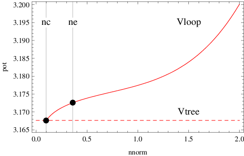
From Eqs. (37) and (38), we obtain for the spectral index and the scale $M$ from the COBE normalization evaluated $50$ e-folds before the end of inflation

$$n_{\text{s}}\simeq 0.982\,,\qquad\frac{M}{M_{\text{P}}}\simeq 3.4\cdot 10^{-3}\,.$$

(39)

This is not within the $68$% CL of the WMAP 5-year data, but still within 95% CL [9]. In addition, the tensor-to-scalar ratio and the running of the spectral index are obtained to be

$$r\simeq 9.0\cdot 10^{-5}\,,\qquad\frac{\text{d}n_{\text{s}}}{\text{d}\ln{k}}\simeq-2.4\cdot 10^{-3}\,,$$

(40)

which are both rather small. As typical for an effective single-field inflation model, the non-Gaussianity parameter $f_{\text{NL}}$ is negligible.

In order to investigate the parameter space, and give the predictions for the spectral index and the tensor-to-scalar ratio in this model, we scan this two-dimensional space. Therefore, we again fix the other parameters and the renormalization scale as above. The results are displayed in Fig. 4. In the upper left corner, the contour lines of the spectral index are plotted over a wider range of the parameter space, where both $\lambda$ and $\kappa$ have been varied from $0$ to $0.2$. The other three plots show contour lines of $n_{\text{s}}$, $r$ and the scale $M/M_{\text{P}}$ in the intervals in which $\lambda$ has been varied from $0$ to $0.04$ and $\kappa$ from $0.2$ to $0.8$, where a minimum of the spectral index has been found. In the shown ranges, the spectral index $n_{s}$ is found to be below $1$, but above about $0.98$. The tensor-to-scalar ratio $r$ is below ${\cal O}(0.01)$, and $M/M_{\text{P}}$ is ${\cal O}(10^{-3})$.

We would like to stress that the above results have been calculated using the minimal model defined in Eqs. (4) and (5) with $f(\rho)$ being of no-scale form as given in Eq. (20). Although the no-scale form is particularly well motivated, in general this assumption might be relaxed and a different function $f(\rho)$ might be chosen. The main requirement for $f(\rho)$ is that the potential for $\rho$ has a minimum of the order of the Planck scale and that the shape of the potential forces $\rho$ to settle rapidly at its minimum. After $\rho$ has settled at its minimum, the values of $f(\rho_{\text{min}})$ and its derivatives affect the normalization of the inflaton field and also the field-dependent masses which finally enter the loop potential. We have analyzed some examples with generalized functions $f(\rho)$ and found that in the considered cases the shape of the potential was not affected and the effects on the observables were small. To give one explicit example, for $f(\rho)=1/\rho$ and $\kappa_{\rho}=-1$, we find a minimum at $\rho_{\text{min}}=(\sqrt{5}-1)/2$ where the modulus stabilizes quickly such that inflation can occur. The minimal value for the spectral index is again around $n_{\text{s}}\sim 0.98$ and the tensor-to-scalar ratio as well as the scale of inflation and the running of the spectral index are only slightly changed. However, a full exploration of general functional dependences of $f(\rho)$ is beyond the scope of the paper.

On the contrary, as noted already in section 2.2, we find that the inclusion of additional couplings, for instance of $\kappa_{SH}\neq 0$ as in Eq. (2), could lower the spectral index at loop-level. The reason is that with such modifications, the form of the potential changes qualitatively compared to Fig. 3. For example, for the parameters $(\kappa,\lambda,\kappa_{SH})=(0.05,0.2,10)$ we find a spectral index of $n_{\text{s}}\simeq 0.953$ at horizon exit where the COBE normalization fixes $M/M_{\text{P}}\simeq 0.0029$.

In this paper we have proposed a class of models in which the $\eta$-problem of SUSY hybrid inflation is resolved using a Heisenberg symmetry, where the associated modulus field is stabilized and made heavy with the help of the large vacuum energy during inflation without any fine-tuning. The proposed class of models is well motivated both from string theory considerations, since it includes the commonly encountered case of no-scale SUGRA Kähler potential, and from the perspective of particle physics since a natural candidate for the inflaton in this class of models is the right-handed sneutrino, i.e. the superpartner of the SM-singlet right-handed neutrino, which is massless during the inflationary epoch and subsequently acquires a large mass at the end of inflation.

In order to illustrate the approach we have developed in some detail a specific example motivated by sneutrino hybrid inflation with no-scale SUGRA. In this example the right-handed sneutrino field $N$ appears in the Heisenberg combination in Eq. (3), the superpotential has the form in Eq. (4), and the Kähler potential has the form in Eq. (5) where in practice we have assumed the no-scale form in Eq. (20). In this model the singlet $S$ is stabilized during inflation due to its non-canonical Kähler potential, and since the right-handed sneutrino contained in $N$ has its mass protected by the Heisenberg symmetry, it becomes a natural candidate for the inflaton, with the associated modulus field stabilized and made heavy with the help of the large vacuum energy during inflation (where we have not addressed the problem of the stability of the modulus after inflation). Because of the Heisenberg symmetry the tree-level potential of the sneutrino inflaton is flat and only lifted by radiative corrections (induced by Heisenberg symmetry breaking superpotential couplings) which we have studied and found to play a key part in the inflationary dynamics.

We have found that in the considered setup the spectral index $n_{s}$ typically lies below $1$ with typical values shown in Fig. 4 for the case of the model defined in Eqs. (4) and (5) with $f(\rho)$ given in Eq. (20). However, the inclusion of additional couplings, for instance of $\kappa_{SH}\neq 0$ as in Eq. (2), could lower the spectral index at the loop-level. For example, for the parameters $(\kappa,\lambda,\kappa_{SH})=(0.05,0.2,10)$ we have found a spectral index of $n_{\text{s}}\simeq 0.953$ and $M$ fixed to $M/M_{\text{P}}\simeq 0.0029$ by the COBE normalization. We expect further changes to the predictions for the observables in other extensions or variants of our simple example model.

In conclusion, the class of SUSY hybrid inflation models proposed here not only solves the $\eta$-problem using a Heisenberg symmetry, and stabilize the associated modulus during inflation, but are also well motivated both from string theory and particle physics, and leads to an acceptable value of the spectral index, while predicting very small tensor modes. The specific example of sneutrino hybrid inflation with no-scale SUGRA is a particularly attractive possibility which deserves further study.

S.F.K. acknowledges partial support from the following grants: PPARC Rolling Grant PPA/G/S/2003/00096; EU Network MRTN-CT-2004-50336; EU ILIAS RII3-CT-2004-506222. S.A. was partially supported by the the DFG cluster of excellence “Origin and Structure of the Universe”. The work of M.B.G. is done as part of the program Ramón y Cajal of the Ministerio de Educación y Ciencias (M.E.C.) of Spain. M.B.G. is also partially supported by the M.E.C. under contract FIS 2007-63364 and by the Junta de Andalucía group FQM 101.

References

- [1] For textbook reviews on inflation see: A. R. Liddle and D. H. Lyth, “Cosmological inflation and large-scale structure,” Cambridge, UK: Univ. Pr. (2000) 400 p; A. D. Linde, “Particle Physics and Inflationary Cosmology,” [arXiv:hep-th/0503203]; V. Mukhanov, “Physical Foundations of Cosmology,” Cambridge, UK: Univ. Pr. (2005) 421 p.
- [2] A. D. Linde, “Axions in inflationary cosmology,” Phys. Lett. B 259, 38 (1991).
- [3] E. J. Copeland, A. R. Liddle, D. H. Lyth, E. D. Stewart and D. Wands, “False vacuum inflation with Einstein gravity,” Phys. Rev. D 49, 6410 (1994) [arXiv:astro-ph/9401011].
- [4] A. D. Linde and A. Riotto, “Hybrid inflation in supergravity,” Phys. Rev. D 56, 1841 (1997) [arXiv:hep-ph/9703209].
- [5] R. Jeannerot, “Inflation in supersymmetric unified theories,” Phys. Rev. D 56, 6205 (1997) [arXiv:hep-ph/9706391].
- [6] M. Bastero-Gil, S. F. King and J. Sanderson, “Preheating in supersymmetric hybrid inflation,” Phys. Rev. D 60, 103517 (1999) [arXiv:hep-ph/9904315].
- [7] G. R. Dvali, Q. Shafi and R. K. Schaefer, “Large scale structure and supersymmetric inflation without fine tuning,” Phys. Rev. Lett. 73, 1886 (1994) [arXiv:hep-ph/9406319].
- [8] E. Komatsu et al. [WMAP Collaboration], “Five-Year Wilkinson Microwave Anisotropy Probe (WMAP) Observations:Cosmological Interpretation,” [arXiv:0803.0547 [astro-ph]].
- [9] G. Hinshaw et. al., “Five-Year Wilkinson Microwave Anisotropy Probe (WMAP) Observations: Data Processing, Sky Maps, and Basic Results,” [arXiv:astro-ph/0803.0732].
- [10] H. Murayama, H. Suzuki, T. Yanagida and J. Yokoyama, “Chaotic inflation and baryogenesis by right-handed sneutrinos,” Phys. Rev. Lett. 70 1912 (1993).
- [11] S. Antusch, M. Bastero-Gil, S. F. King, Q. Shafi, “Sneutrino Hybrid Inflation in Supergravity,” Phys. Rev. D71 083519 (2005) [arXiv:hep-ph/0411298].
- [12] M. Dine, L. Randall and S. D. Thomas, “Supersymmetry breaking in the early universe,” Phys. Rev. Lett. 75 (1995) 398;
- [13] H. Murayama, H. Suzuki, T. Yanagida and J. Yokoyama, “Chaotic inflation and baryogenesis in supergravity,” Phys. Rev. D 50, 2356 (1994) [arXiv:hep-ph/9311326].
- [14] M. Kawasaki, M. Yamaguchi and T. Yanagida, “Natural chaotic inflation in supergravity,” Phys. Rev. Lett. 85, 3572 (2000) [arXiv:hep-ph/0004243].
- [15] M. Yamaguchi and J. Yokoyama, “New inflation in supergravity with a chaotic initial condition,” Phys. Rev. D 63, 043506 (2001) [arXiv:hep-ph/0007021].
- [16] P. Brax and J. Martin, “Shift symmetry and inflation in supergravity,” Phys. Rev. D 72, 023518 (2005) [arXiv:hep-th/0504168].
- [17] P. Binetruy and M. K. Gaillard, “Non-Compact Symmetries and Scalar Masses in Superstring-Inspired Models,” Phys. Lett. B195 382-388 (1987).
- [18] M. K. Gaillard, H. Murayama and K. A. Olive, “Preserving flat directions during inflation,” Phys. Lett. B 355, 71 (1995) [arXiv:hep-ph/9504307].
- [19] R. Brustein and P. J. Steinhardt, “Challenges for superstring cosmology,” Phys. Lett. B 302, 196 (1993) [arXiv:hep-th/9212049].
- [20] M. Dine, “Towards a solution of the moduli problems of string cosmology,” Phys. Lett. B 482 (2000) 213 [arXiv:hep-th/0002047].
- [21] J. R. Ellis, Z. Lalak, S. Pokorski and K. Turzynski, “The price of WMAP inflation in supergravity,” JCAP 0610, 005 (2006) [arXiv:hep-th/0606133].
- [22] S. C. Davis and M. Postma, “SUGRA chaotic inflation and moduli stabilisation,” JCAP 0803, 015 (2008) [arXiv:0801.4696 [hep-ph]].
- [23] L. Covi, M. Gomez-Reino, C. Gross, J. Louis, G. A. Palma and C. A. Scrucca, “Constraints on modular inflation in supergravity and string theory,” JHEP 0808, 055 (2008) [arXiv:0805.3290 [hep-th]].
- [24] P. Brax, C. van de Bruck, A. C. Davis and S. C. Davis, “Coupling hybrid inflation to moduli,” JCAP 0609, 012 (2006) [arXiv:hep-th/0606140].
- [25] S. C. Davis and M. Postma, “Successfully combining SUGRA hybrid inflation and moduli stabilisation,” JCAP 0804, 022 (2008) [arXiv:0801.2116 [hep-th]].
- [26] M. K. Gaillard, D. H. Lyth and H. Murayama, “Inflation and flat directions in modular invariant superstring effective theories,” Phys. Rev. D 58, 123505 (1998) [arXiv:hep-th/9806157].
- [27] E. D. Stewart, “Inflation, Supergravity and Superstrings,” Phys. Rev. D51 6847-6853 (1995) [arXiv:hep-ph/9405389].
- [28] S. Ferrara, C. Kounnas, F. Zwirner, “Mass Formulae and Natural Hierarchy in String Effective Supergravities,” Nucl. Phys. B429 589 (1994) [arXiv:hep-th/9405188].
- [29] R. Kallosh, S. Prokushkin, “SuperCosmology,” SU-ITP-04/09 [arXiv:hep-th/0403060].
- [30] S. Coleman, E. Weinberg, “Radiative Corrections as the Origin of Spontaneous Symmetry Breaking,” Phys. Rev. D7 1888 (1973).
- [31] S. Weinberg, “Perturbative Calculations Of Symmetry Breaking,” Phys. Rev. D 7, 2887 (1973).
- [32] G. Gamberini, G. Ridolfi and F. Zwirner, “On Radiative Gauge Symmetry Breaking in the Minimal Supersymmetric Model,” Nucl. Phys. B 331, 331 (1990).