Diffusion in confined geometries
Abstract
Diffusive transport of particles or, more generally, small objects
is a ubiquitous feature of physical and chemical reaction systems.
In configurations containing confining walls or constrictions
transport is controlled both by the fluctuation statistics of the
jittering objects and the phase space available to their dynamics.
Consequently, the study of transport at the macro- and nanoscales
must address both Brownian motion and entropic effects. With this
survey we report on recent advances in the theoretical and numerical
investigation of stochastic transport occurring either in
micro-sized geometries of varying cross section or in narrow
channels wherein the diffusing particles are hindered from passing
each other (single file diffusion). For particles undergoing biased
diffusion in static suspension media enclosed by confining
geometries, transport exhibits intriguing features such as (i) a
decrease of nonlinear mobility with increasing temperature or, also,
(ii) a broad excess peak of the effective diffusion above the free
diffusion limit. These paradoxical aspects can be understood in
terms of entropic contributions resulting from the restricted
dynamics in phase space. If, in addition, the suspension medium is
subjected to external, time-dependent forcing, rectification or
segregation of the diffusing Brownian particles becomes possible.
Likewise, the diffusion in very narrow, spatially modulated channels
gets modified via contact particle-particle interactions, which
induce anomalous sub-diffusion. The effective sub-diffusion constant
for a driven single file also develops a resonance-like structure as
a function of the confining coupling constant.
Keywords: diffusive transport, Brownian motion, entropic effects, diffusion enhancement, single
file diffusion
1 Introduction
Effective control of transport in artificial micro- and nano-structures requires a deep understanding of the diffusive mechanisms involving small objects and, in this regard, an operative measure to gauge the role of fluctuations. Typical such situations are encountered when studying the transport of particles in biological cells [1] and in zeolites [2], catalytic reactions occurring on templates or in porous media [3], chromatography or, more generally, separation techniques of size disperse particles on micro- or even nanoscales [4]. To study these transport phenomena is in many respects equivalent to studying geometrically constrained Brownian dynamics [5, 6, 7]. The fact that the diffusion equation is closely related to the time evolution of the probability density to find a jittering particle at a location at time dates back to Einstein’s pioneering work on the molecular-kinetic description of suspended particles [8].
With this minireview we focus on the problem of the diffusion of small size particles in confined geometries. Restricting the volume of the phase space available to the diffusing particles by means of confining boundaries or obstacles originates remarkable entropic effects [9]. The driven transport of charged particles across bottlenecks, such as ion transport through artificial nanopores or artificial ion pumps [10, 11, 12, 13] or in biological channels [14, 15, 16, 17, 18] is the better known model where diffusion is determined by entropic barriers. Similarly, the operation of artificial Brownian motors [19, 20, 21], molecular motors [22] and molecular machines [23] also results from the interplay of diffusion and binding action by energetic or, more relevant in the present context, entropic barriers [24]. The efficiency of such nanodevices crucially depends on the fluctuation characteristics of the relevant degrees of freedom [25]. In addition, the interplay of diffusion over entropic barriers and unbiased time periodic drives is responsible for certain paradoxical transport effects, like the recent observation of entropic-diffusion controlled absolute negative mobility [26].
Although we restricted ourselves to small size particle, we remind the reader that entropic forces surely affect the dynamics of extended chains diffusing on a periodic two (2D) or three dimensional (3D) substrate. A well established example is represented by the phonon damping of propagating solitons [27]. Another example of great interest for its potential applications in nanotechnology is the translocation of a long polymer molecule through a pore with opening size comparable with the polymer gyration radius. In this case, entropic effects were first predicted to theoretically describe the conformation changes the chain undergoes to move past a conduit constriction [28] and, then, experimentally observed both in biological [29] and artificial channels [30].
Another instance of constrained Brownian dynamics that rests, indeed, within the scopes of our minireview, is the so-called single file diffusion. The motion of an assembly of small size particles in a narrow channel can be so tightly restricted in the transverse directions that the particles arrange themselves into a single file. The longitudinal motion of each particle is thus hindered by the presence of its neighbors, which act as nonpassing movable obstacles. As a consequence, interparticle interactions in one dimension can suppress Brownian diffusion and lead to the emergence of a new subdiffusive dynamics [31].
The outline of this work is as follows. In Sec. 2 we detail the geometry of the channels relevant to our review and set up the mathematical formalism needed to model the diffusion of a Brownian particle immersed in a confined suspension fluid. In Sec. 3 we introduce some exact results for the mobility and the diffusion coefficient of a driven Brownian particle in a one dimensional (1D) periodic potential, results that will be handy in the subsequent sections. In Sec. 4 we compute explicitly the entropic effects on particle transport in a static fluid filling a periodically modulated channel. In Sec. 5 we address particle transport in a suspension fluid flowing along the channel subject to stationary pumping. In Sec. 6 we review numerical and analytical results for the diffusion of a single file along a periodically corrugated channel both in the presence and in the absence of an external drive.
2 Channel models

We consider the diffusive dynamics of spherical particles in 2D or 3D pores, or channels, which extend in the direction and possess a periodically varying cross section. These channels are supposed to be symmetric with respect to a reflection on the channel axis in 2D (like those sketched in Fig. 1), or to any rotation about the channel axis in 3D. The channels are assumed to be delimited by rigid, smooth walls. The half width of the channel is described by the well-behaved boundary function . The channel walls do confine the particles inside the channel but, otherwise, do not exchange energy with them. In particular, we do not consider the possibility of adsorption of particles at the walls. Since we will disregard any rotatory motion of the particles about their centers of mass, we need not specify particle-wall contact forces. Moreover, the radius of the particles is supposed to be smaller than the minima of (channel bottlenecks), so that the particles are not restricted to stay within a confined region of the channel, but rather may diffuse everywhere along the channel.
2.1 Diffusion equations
The motion of particles that are immersed in a fluid medium may be influenced by various types of forces. We will here restrict ourselves to the discussion of small radius (almost pointlike) particles, whose presence does not significantly modify the free motion of the fluid around them (laminar flow regime). The systematic impact of the fluid on the motion of particles at position is given by the Stokes force [32]
| (1) |
where is the instantaneous velocity of the fluid in absence of the particle, is the instantaneous particle velocity, and
| (2) |
is the friction constant, which is determined by the shear viscosity of the fluid, and the radius of the particle. At the same time the fluid exerts on the particle also a random thermal force . In the following, we only deal the case of fluids with homogeneous temperature and velocity fields that are almost constant on the particle scale . As a consequence, to insure thermalization at temperature it suffices to set
| (3) |
where denotes the Boltzmann constant and is a standard 3D Gaussian noise with and for . Other forces acting on the particles, like hydrodynamic interactions among different particles and between single particles and the wall, will be neglected [33, 34]. This simplification, in particular, requires a sufficiently low particle density.
Finally, an external force may act on the particles describing e.g. the gravity force, or in the case of charged particles, an electrostatic force. We further specialize our discussion to constant longitudinal external forces pointing in the direction of the symmetry axis of the channel. The dynamics of the center of mass of a single particle is then governed by Newton’s equation of motion
| (4) |
where we explicitly allow for a possible time-dependence of the fluid velocity field. For microparticles moving with typical velocities of the order of 1 cm/s, the inertial term in Eq. (4) is negligibly small compared to the environmental forces [35]; therefore, provided that the fluid velocity does not changes too fast, that is for spectral frequencies less than a few 100 Hz, one can safely set (overdamped limit or Smoluchowski approximation). Under these conditions the equation of motion (4) can be simplified as
| (5) |
This Langevin equation is equivalent to the following Fokker-Planck equation [36] for the probability density of a particle to be found at the position at time :
| (6) |
Here denotes the corresponding probability current density
| (7) |
These equations have to be supplemented by appropriate boundary conditions, which will be discussed in the following subsection.
2.2 Boundary conditions
The channel is typically characterized by two boundary regions: A transverse boundary naturally results from the presence of the walls, whereas a longitudinal boundary is required to account for the channel length.
The probability flux normal to the boundary in the presence of a rigid hard wall must vanish. Thus, to prevent pointlike particles from leaving the channel or being adsorbed at the walls, we must impose that
| (8) |
where denotes the unit vector normal to the wall at point . Note, however, that the center of mass of a spherical particle of finite radius may approach the wall only up to a distance , so that for finite size particles the boundary conditions (8) applies on an appropriate inner surface parallel to the channel walls [37].
Various kinds of boundary conditions exist that regulate the inward and outward probability flows at the ends of a channel [32]. If the channel connects large, well mixed particle reservoirs, then constant probability densities may be assigned at the channel ends. This leads to Dirichlet boundary conditions of the form
| (9) |
where and denote respectively the left and right endpoints of the channel. A more detailed description of the particle flow into and out of a channel can be achieved by relating flux and probability densities at , that is [38]
| (10) |
Here, positive (negative) constants correspond to partially absorbing (emitting) boundaries. As special cases, reflecting and absorbing boundaries correspond to and , respectively.
3 Exact results for 1D systems
In order to set the stage, we consider first the ideal case where the diffusion of a particle in a periodically corrugated channel can be assimilated to the diffusion on an energetic landscape represented, for simplicity, by a 1D periodic substrate with period , namely . Such a model is often employed to model, for instance, nanotube [39] and zeolite diffusion [2]. Let us consider a Brownian particle with mass , coordinate , and friction coefficient , subjected to a static external force and a thermal noise . In the notation of Sec. 2.1, we set .
The corresponding stochastic dynamics is described by the Langevin equation
| (12) |
where is the standard Gaussian noise also defined in Sec. 2.1. Moreover, for the purposes of this review, the substrate can be taken symmetric under reflection, .
In extremely small systems, particle fluctuations are often described to a good approximation by the overdamped limit of Eq. (12), i.e., by the massless Langevin equation
| (13) |
where the inertia term has been dropped altogether (Smoluchowski approximation).
An overdamped particle is trapped most of the time at a local minimum of the tilted substrate as long as , denoting the depinning threshold . Drift occurs by rare noise induced hopping events between adjacent minima. For there exist no such minima and the particle runs in the direction with average speed approaching the no-substrate limit . This behavior is described quantitatively by the mobility formula:
| (14) |
with
| (15) |
Here and in the following, denotes the -th moment of the first passage time of the particle across a substrate unit cell in the direction.
As the particle drifts subjected to the external force , the random hops cause a spatial dispersion of the particle around its average position . The corresponding normal diffusion coefficient,
| (16) |
can be computed analytically by regarding the hopping events in the overdamped regime as manifestations of a renewal process, that is [40]:
| (17) |
Simple algebraic manipulations lead to explicit expressions for the nonlinear mobility [36, 41, 42, 43],
| (18) |
and for the diffusion coefficient [40],
| (19) |
Here, and denotes Einstein’s coefficient for a free diffusing Brownian particle.
For Eqs. (18) and (19) reproduce the zero-bias identity with [36, 44]. Notably, as approaches the depinning threshold the mobility curve (18) jumps from zero (locked state) up to close (running state). Correspondingly, the diffusion coefficient (19) develops a diffusion excess peak, i.e. with , consistently with numerical observations in Ref. [45]. Both the mobility step and the peak get sharper and sharper as is lowered [40]. The same conclusions apply in the presence of inertia (i.e. for particles of finite mass ) [45, 46], as well, with the difference that the relevant depinning threshold shifts towards lower values (proportionally to as [36]).
Finally, we emphasize that the above formulas for the nonlinear mobility and the effective diffusion coefficient retain their analytic structure also when generalized to anomalous (sub)-diffusion on a 1D substrate, by merely substituting the normal diffusion constant by the fractional diffusion constant occurring in the corresponding fractional diffusion equation [47].
4 Particle diffusion in a static fluid
In the limiting case of pointlike particles with zero interaction radius diffusing in constrained 2D or 3D geometries, elastic contact particle-particle interactions can be neglected. As long as hydrodynamically mediated interactions can also be neglected, see e.g. [33, 34], the confining action of the channel walls is modeled by the perfectly reflecting boundary conditions (8).
In the presence of a constant external force pointing in the channel direction, an overdamped Brownian particle suspended in a static medium is described by the Langevin equation (5), or by the corresponding Fokker-Planck equation (6), both with zero velocity field . For a general choice of the periodic boundary , there exist no exact analytical solutions to the Fokker-Planck equation (6) with boundary conditions (8). However, approximate solutions can be obtained by reducing the problem of free Brownian diffusion in a 2D or 3D channel to that of Brownian diffusion on an effective 1D periodic substrate (Sec. 3). Under such a scheme, narrow channel constrictions, corresponding to geometric hindrances in the fully dimensional problem, are modeled as entropic 1D barriers.
In the absence of external forces, i.e., for , particle dynamics in confined structures [see Fig. 1(a)] can be approximately described by the Fick-Jacobs kinetic equation with spatially dependent diffusion coefficient [48, 49, 50, 51]:
| (20) |
with denoting the dimensionless channel cross-section in 2D and in 3D. Equation (20) was obtained [49] from the full Fokker-Planck equation (6) for small amplitude boundary modulations , on assuming a uniform density and integrating out the transverse coordinates [e.g. for a 2D channel ]. At variance with the original Fick-Jacobs equation [48], introducing an -dependent diffusion coefficient considerably improved the accuracy of the kinetic equation (20) thus extending its validity to larger amplitudes [49, 50, 51]. Here, the expression
| (21) |
with in 2D and in 3D, was determined to best account for wall curvature effects [50, 52].
In the presence of weak longitudinal drives , the Fick-Jacobs equation (20) can be further extended to [50, 52, 53]:
| (22) |
where the free energy is made up of an energy, , and an entropic term, . For a periodic channel, assumes the form of a tilted periodic potential. Moreover, for a straight channel, , the entropic contribution vanishes altogether and the particle is subject to the sole external drive. Of course, for the free energy is purely entropic and Eq. (22) reduces to the Fick-Jacobs equation (20). An alternative reduction scheme based on macrotransport theory has been proposed recently in Ref. [54].
Key quantifiers of the reduced 1D kinetics (22) are the average particle current or, equivalently, the nonlinear mobility (14), and the effective diffusion coefficient (17) defined in Sec. 3. On generalizing the derivation of Eqs. (18) and (19) to account for the -dependence of , one obtains [53], respectively,
| (23) |
and
| (24) |
where
| (25) |
and the dimensionless force is defined as the ratio of the work done by to drag the particle a distance , to the thermal energy , that is
| (26) |
We stress here an important difference with the energetic 1D model of Sec. 3. For a particle moving in a 1D periodic substrate , the barriers separating the potential wells provide an additional energy scale besides and , so that the particle dynamics is governed by at least two dimensionless energy parameters, say, and [36]. In contrast, Brownian transport in a periodically corrugated 2D or 3D channel is solely determined by the dimensionless force [53]. This can be proven by rescaling the problem units as follows. We measure all lengths in units of the period and time in units of , that is, twice the time the particle takes to diffuse a distance at temperature . In these new dimensionless variables the Langevin equation (5) for a Brownian particle in a static medium reduces to the equation
| (27) |
with no tunable constants [55]. As a consequence, the ensuing Brownian dynamics is controlled only by the parameter and, of course, by the additional length(s) that possibly enter the boundary function .
The -dependence of the average particle current (23) and the effective diffusion (24) were compared with the results obtained by numerical integration of the 2D Langevin equation (5) (for details see Ref. [52]). For simplicity, the channel walls were assumed to have the sinusoidal profile
| (28) |
with and . Here, are, respectively, the maximum and the minimum channel width. Moreover, controls the slope of the boundary function , which in turn determines the modulation amplitude of the diffusion coefficient in Eq. (21). The mobility , Eq. (14), and the corresponding effective diffusion coefficient , Eq. (16), were computed by ensemble averaging simulated trajectories.


The most significant results are displayed in Figs. 2 and 3. At variance with the purely energetic 1D models of Sec. 3, the nonlinear mobility decreases upon increasing the strength of thermal noise. Moreover, an enhancement of the effective diffusion coefficient, with maximum exceeding the free diffusion constant , was also observed [53, 55].
At low values of the control parameter the analytical approximations (23) and (24) match perfectly the corresponding numerical curves, whereas deviations occur at high . Most remarkably, contrary to the simulation output, the analytical curves for and fail to attain the correct asymptotic limit for (see insets in Figs. 2 and 3). This occurs because the assumption of uniform density distribution, introduced in the Fick-Jacobs formalism to eliminate the transverse coordinates, is no more tenable in the presence of strong drives.
The agreement between theory and numerics improves for smooth
modulations of the channel walls, i.e. for small boundary slopes
, which can be achieved, e.g., for appropriately
small [52, 55]. A phenomenological
criterion to asses the validity of the stationary state solutions of
the Fick-Jacobs equation (22) can be
formulated by comparing the different characteristic time scales of
the problem, namely
(i) the diffusion times, respectively, in the
transverse,
| (29) |
(ii) and in the longitudinal direction,
| (30) |
(iii) and the drift time the applied force takes to drag the particle one channel unit length across,
| (31) |
Uniform probability distribution in the transverse direction sets on only if the transverse diffusion motion of the particle is sufficiently fast relative to both the diffusive and the drift longitudinal motions, which implies . For large drives it suffices to require that , which leads to the condition [55]:
| (32) |

The critical force parameter , above which the Fick-Jacobs description is expected to fail, depends on the remaining free parameters of the problem. For the boundary function (28), is a function of , alone, as illustrated in Fig. 4. For the Fick-Jacobs approximation becomes untenable already for relatively small forces , whereas for its validity extends to significantly larger drives.
5 Particle diffusion in moving fluids
Let us assume now that a small, spherical particle is swept along in the stationary velocity field of a moving, incompressible fluid [see Fig. 1(b)], rather than by a constant force, , like in Sec. 4. For , its dynamics is then described by the Langevin equation, in the overdamped limit,
| (33) |
where the fluid velocity field is to be determined.
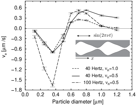
To this purpose, we write first the Stokes equations for a stationary incompressible flow in the limit of vanishing Reynolds numbers (the convective acceleration terms in the Navier-Stokes equations can be safely neglected). One obtains the so-called “creeping flow equation” [32]: where is the pressure field responsible for the stationary laminar flow of the fluid and is the absolute dynamic fluid (or shear) viscosity. On introducing the scalar field , with being the polar coordinates in the transverse plane , can be rewritten as [32]
| (34) |
where is the unit vector. On substituting Eq. (34) into the creeping flow equation, one obtains the following linear homogeneous fourth-order differential equation [32, 56]:
| (35) |
with boundary conditions
| (36) | |||
| (37) | |||
| (38) | |||
| (39) |
where is an arbitrary constant. Solutions to Eq. (35), determine the velocity field up to a multiplicative factor, which, in turn, can be established by imposing some additional condition, e.g. for the pressure drop across a channel unit, i.e. [56]
| (40) |
Once the velocity field for a particular channel geometry and pressure profile is known, the Langevin equation (33) can be solved numerically.
Particle separation across a micro-channel is a process of great technological importance [7, 19]. Any inhomogeneity in the spatial distribution of an ensemble of non-interacting suspended particles can only be caused by the hydrodynamic interaction between particles and walls [37]. The no-flux boundary condition (8) for unbiased particles with reads:
| (41) |
In the case of vanishing drift velocity normal to the channel walls, , only uniform distributions are allowed and no particle separation could ever be achieved [37]. However, as anticipated in Sec. 2.2, for finite size particles the no-flux boundary condition (41) strictly holds on an effective inner surface at a distance from the channel walls. Due to its finite size, a particle cannot move steadily along a given flow streamline as this gets too close to the walls; upon hitting the wall, the particle bounces into inner flow streamlines as if they were subject to a transverse field gradient. These hydrodynamic forces may, indeed, lead to accumulation and depletion zones within the channel.
By generalizing such a boundary effect, Kettner et al. [56] predicted by numerical simulation that a micron-sized channel with broken reflection symmetry can be used to separate particles according to their size, as illustrated in Fig. 5. A time oscillating pressure profile, , where is a sinusoidal function with frequency , was assumed to control the periodic flow of the fluid, back and forth along an infinitely long channel. Within the creeping flow approximation, the ensuing time dependent velocity field was then obtained in terms of the solution of the unperturbed Stokes equation introduced above, and the corresponding Langevin equation (33) numerically integrated. Later on, this mechanism was demonstrated experimentally by Matthias and Müller [57].
6 Single File Diffusion
As the design and the operation of biology inspired nanodevices [19] have become experimentally affordable, understanding particle diffusion in a 1D substrate has been recognized as a key issue in transport control [25]. In this context the particle- and particle-wall interactions play a central role. Pair interaction between thermally diffusing particles does not affect the normal character of Brownian diffusion, as long as the particles are able to pass one another, no matter how closely they are confined. This holds true even when, under appropriate temperature and density conditions, attracting particles cluster or condense in the substrate wells [58].
Things change dramatically for strictly 1D geometries. Let us consider, for instance, an ensemble of unit-mass particles moving with preassigned dynamics along a segment of length . If the interparticle interaction is hard-core (with zero radius), the elastic collisions between neighboring particles are nonpassing – meaning that the particles can be labeled according to a fixed ordered sequence. The particles are thus arranged into a file where, at variance with the situation described in Sec. 2, their diffusion is suppressed by the presence of two nonpassing neighbors, also movable in the longitudinal direction.

The diffusion of a free single file (SF), i.e. in the absence of a substrate, has been investigated in detail [31]. In the thermodynamic limit ( with constant density ) the mean square displacement of each file particle can be written as
| (42) |
with denoting the absolute mean displacement of a free particle. For a ballistic single file (bSF), clearly , where is the ensemble average taken over the distribution of the initial velocities, and therefore
| (43) |
A bSF particle diffuses apparently like a Brownian particle with normal diffusion coefficient . For a stochastic single file (sSF) of Brownian particles with damping constant at temperature , the equality yields the anomalous diffusion law
| (44) |
where the mobility factor is related to the single particle diffusion constant . The onset of the subdiffusive regime (44) occurs for , being the average time a single particle takes to diffuse against one of its neighbors [59, 60]. The diffusive regimes (43) and (44) have been demonstrated both numerically [61] and experimentally [34, 62].

Let represent the coordinate of one file particle, assumed to be a continuous differentiable stochastic process with . Kubo’s relation [63]
| (45) |
with , best illustrates the role of the dimensional constraint on SF diffusion. In the case of normal diffusion, , the r.h.s. of Eq. (45) converges to the positive value , namely diffuses subject to Einstein’s law. The subdiffusive dynamics (44), instead, is characterized by , which, in view of Eq. (45), implies that develops a negative power-law tail with and . Numerical simulations support this conclusion. In Fig. 6 we report a few curves for different and . The negative tails are apparent and compare well with the estimate derived from Eq. (45) (see inset). They are a typical signature of the collisional dynamics in a SF: As an effect of pair collisions, an initial velocity is likely to be compensated by a backflow velocity of opposite sign [60, 64].
6.1 Stochastic single file on a substrate
We focus now on the case of a SF diffusing on a sinusoidal substrate with potential [65, 66]
| (46) |
This variation of the SF model rises naturally in connection with quasi-1D situations where the particles (not necessarily suspended in a fluid) can be represented by disks moving along a narrow spatially modulated channel with cross-section smaller than twice the disk diameter [see Fig. 1(c)]. The confining action of the channel can be accounted for by modeling the SF dynamics in terms of a periodic substrate potential with a effective strength . This is the case, for instance, of most nanotubes and zeolite pores [2].
In the simulations of Refs. [60, 66] the -th particle was assigned: (i) random initial position, , and velocity, . Upon each elastic collision it switched velocity with either neighbors without altering the file labeling; (ii) independent Brownian dynamics determined by a viscous force and a thermal force , with uncorrelated standard Gaussian noises defined as in Sec. 2.1, in order to guarantee thermalization at temperature .
Numerical evidence led to conclude that the periodic substrate potential does not invalidate the sSF diffusion law (44), although the dependence of the mobility factor on the system parameters becomes more complicated. In panels (a) and (b) of Fig. 7 is characterized as a function of and , respectively. The identity , reported above for , applies here, too, under the condition of replacing with the modified diffusion constant of Eq. (19). In Fig. 7(a) the rescaled curves versus overlap asymptotically for any damping regime.
The temperature dependence of the mobility , is more interesting. As implicit in the discussion of Sec. 3, this prediction gets more and more accurate for large and increasingly high activation-to-thermal energy ratios . As a consequence, the rescaled mobility turns out to be a function of , alone, in good agreement with the simulation results displayed in Fig. 7(c).

6.2 Driven single files
Finally, we consider the case of a driven sSF, namely, we now assume that all file particles are subjected to an additional constant force pointing, say, to the right (). We know from Sec. 3 that the diffusion of a single Brownian particle drifting down a tilted washboard potential exhibits enhanced normal diffusion with diffusion constant (19). Extensive simulation of a driven SF [66] yielded the numerical data reported in Fig. 8. The kinetic mobility of the file, defined as , turned out to coincide with the mobility of a single particle under the same dynamical conditions, irrespective of (inset of Fig. 8). More remarkably, the subdiffusive regime (44) applies also in the presence of bias, though with an -dependent mobility factor. When plotted versus , attained a maximum enhancement for , i.e., in coincidence with the (noise-assisted) depinning of the file from its sinusoidal substrate. Again, the identity combined with formula (19) for provided an excellent fit of the simulation data for large . Of course, the mobility enhancement at depinning can be revealed also by plotting versus at constant .
7 Conclusions and Outlook
With this minireview we presented the state of the art of diffusive transport occurring in systems characterized by confinement due to either their finite size or to particle interactions in restricted geometries. Confinement plays a salient role in the Brownian motion of driven particles. Indeed, the entropic effects associated with confinement may give rise to anomalous transport features. Some main new phenomena are the entropy-driven decrease of mobility with increasing temperature, the diffusion excess above the free diffusion limit and the resonant behavior of the effective diffusion coefficient as a function of control parameters such as temperature, external gradients, or geometry design.
The reviewed transport features can thus be implemented in the design of new transport control setups or protocols. In particular, Brownian transport through confined geometries is expected to find application in nanotechnology, for instance, to operate devices for the separation of nanoparticles, to speed up schemes for catalysis on templates, or also to realize efficient, driven through-flows of microsized agents, or reactants, in miniaturized lab-on-a-chip devices.
Acknowledgements
This work was made possible thanks to the financial support by: the Volkswagen Foundation (project I/80424, P.H.); the Deutsche Forschungsgemeinschaft (DFG) via project no. 1517/26-1 (P.S.B., P.H.) and via the research center, SFB-486, project A10 (G.S., P.H.); the German Excellence Initiative, via the Nanosystems Initiative Munich (NIM) (P.S.B., P.H.); and the Alexander von Humboldt Stiftung, via a Research Award (F.M.).
References
- [1] B. Alberts, A. Johnson, J. Lewis, M. Raff, K. Roberts, P. Walter, Molecular Biology of the Cell, Garland, New York, 2007.
- [2] J. Kärger, D. M. Ruthven, Diffusion in Zeolites and Other Microporous Solids, Wiley, New York, 1992.
- [3] M. C. Daniel, D. Astruc, Chem. Rev. 1997, 104, 293-346.
- [4] A. Corma, Chem. Rev. 1997, 97, 2373-2419.
- [5] R. M. Mazo, Brownian Motion: Fluctuations, Dynamics and Applications (Clarendron Press, Oxford 2002).
- [6] P. Hänggi, F. Marchesoni, Chaos 2005, 15, 026101.
- [7] P. Hänggi, F. Marchesoni, Rev. Mod. Phys. 2009, arXiv:0807.1283.
- [8] A. Einstein Ann. Physik (Leipzig) 1905, 17, 549-560.
- [9] L. Liu, P. Li, S. A. Asher, Nature 1999, 397, 141-144.
- [10] Z. Siwy, I. D. Kosinska, A. Fulinski, C. R. Martin, Phys. Rev. Lett. 2005, 94, 048102.
- [11] Z. Siwy, A. Fulinski Am. J. Phys. 2004 72, 567-574.
- [12] A. M. Berezhkovskii, M. A. Pustovoit, S. M. Bezrukov J. Chem. Phys. 2007, 126, 134706.
- [13] I. D. Kosinska, I. Goychuk, M. Kostur, G. Schmid, P. Hänggi, Phys. Rev. E 2008, 77, 031131.
- [14] A. M. Berezhkovskii, S. M. Bezrukov, Biophys. J. 2005, 88, L17-L19.
- [15] A. M. Berezhkovskii, S. M. Bezrukov, Phys. Rev. Lett. 2008, 100, 038104.
- [16] W. Nonner, B. Eisenberg J. Mol. Liquids 2000, 87, 149-162
- [17] D. Gillespie, W. Nonner, R. S. Eisenberg J. Phys. -Cond. Mat. 2002, 14, 12129-12145.
- [18] D. Boda, D. D. Busath, B. Eisenberg, D. Henderson, W. Nonner PhysChemChemPhys 2002 4, 5154-5160.
- [19] P. Hänggi, F. Marchesoni, F. Nori, Ann. Physik (Berlin) 2005, 14, 51-70.
- [20] R. D. Astumian, P. Hänggi, Physics Today 2002, 55 (11), 33-39.
- [21] P. Reimann, P. Hänggi, Appl. Physics A 2002, 75, 169-178.
- [22] E. R. Kay, D. A. Leigh, F. Zerbetto, Angew. Chem. Int. Ed. 2007, 46, 72-191.
- [23] V. Balzani, A. Credi, M. Venturi, ChemPhysChem 2008, 9, 202-220.
- [24] a) I. Derenyi, R. D. Astumian, Phys. Rev. E 1998, 58, 7781-7784; b) T. A. J. Duke, R. H. Austin, Phys. Rev. Lett. 1998, 80, 1552-1555; c) A. Van Oudenaarden, S. G. Boxer, Science 1999, 285, 1046-1048; d) M. Kostur, L. Schimansky-Geier, Phys. Lett. 2000, 265, 337-345; e) C. Keller, F. Marquardt, C. Bruder, Phys. Rev. E 2002, 65, 041927.
- [25] L. Machura, M. Kostur, P. Talkner, J. Luczka, F. Marchesoni, P. Hänggi, Phys. Rev. E 2004, 70, 061105.
- [26] a) R. Eichhorn, P. Reimann, P. Hänggi Phys. Rev. Lett. 2002, 88, 190601; Phys. Rev. E 2002, 66, 066132; b) L. Machura, M. Kostur, P. Talkner, J. Luczka, P. Hänggi Phys. Rev. Lett. 2007, 98, 040601; c) M. Kostur, L. Machura, P. Talkner, P. Hänggi, J. Luczka Phys. Rev. B 2008, 77, 104509.
- [27] a) J. Currie, J. A. Krumhansl, A. R. Bishop, S. E. Trullinger, Phys. Rev. B 1980, 22, 477-496; b) G. Costantini, F. Marchesoni, Phys. Rev. Lett. 2001, 87, 114102.
- [28] E. Arvanitidou, D. Hoagland, Phys. Rev. Lett. 1991, 67, 1464-1466.
- [29] J.J. Kasianowicz, E. Bradin, D. Branton, D. W. Deemer Proc. Natl. Acad. Sci. 1996, 93 13770-13773.
- [30] a) J. Han, S. W. Turner, H. G. Craighead, Phys. Rev. Lett. 1999, 83, 1688-1691; b) J. Han, H. G. Craighead, 2000, Science 2000, 288, 1026-1029.
- [31] a) D. W. Jepsen, J. Math. Phys. 1965, 6, 405-413; b) D. G. Levitt, Phys. Phys. A 1973, 8, 3050-3054; c) T. E. Harris, Ann. Prob. 1974, 2, 969-988; d) J. K. Percus, Phys. Phys. A 1974, 9, 557-559.
- [32] a) H. Lamb Hydrodynamics, Dover Publications, New York, 1945; b) L. G. Leal Laminar Flow and convective transport, Butterworth-Heinmann, Boston, 1992; c) Z. U. A. Warsi Fluid dynamics, CRC Press, Boca Raton, FL, 1992.
- [33] B. Cui, H. Diamant, B. Lin Phys. Rev. Lett. 2002, 89, 188302.
- [34] Q. H. Wei, C. Bechinger, P. Leiderer, Science 2000, 287, 625-627.
- [35] E. M. Purcell, Am. J. Phys. 1977, 45, 3-11.
- [36] H. Risken The Fokker-Planck Equation, 2nd ed., Springer, Berlin, 1989.
- [37] M. Schindler, P. Talkner, P. Hänggi, Physica A 2007, 385, 46.
- [38] S. M. Bezrukov, A. M. Berezhkovskii, M. A. Pustovoit, A. Szabo J. Chem. Phys. 2000, 113, 8206-9211.
- [39] M. S. Dresselhaus, G. Dresselhaus, P. C. Eklund, The Science of Fullerenes and Carbon Nanotubes, Academic, New York, 1996.
- [40] P. Reimann, C. Van den Broeck, H. Linke, P. Hänggi, J. M. Rubí, A. Pérez-Madrid, Phys. Rev. Lett. 2001, 87, 010602; Phys. Rev. E 2002, 65, 031104.
- [41] R. L. Stratonovich Radiotekhnika i elektronika (Moscow) 1958, 3, 497-511.
- [42] V. I. Tikhonov Avtom. Telemekh. 1959, 20, 1188-1196.
- [43] P. Hänggi, P. Talkner, M. Borkovec, Rev. Mod. Phys. 1990, 62, 251-342.
- [44] S. Lifson, J. L. Jackson J. Chem. Phys. 1962, 36, 2410-2414.
- [45] G. Costantini, F. Marchesoni, Europhys. Lett. 1999, 48, 491-497.
- [46] C. Cattuto, G. Costantini, T. Guidi, F. Marchesoni, Phys. Rev. B 2001, 63, 094308.
- [47] a) I. Goychuk, E. Heinsalu, M. Patriarca, G. Schmid, P. Hänggi Phys. Rev. E 2006, 73, 020101(R); b) E. Heinsalu, M. Patriarca, I. Goychuk, P. Hänggi J. Phys.: Cond. Matter 2007, 19, 065114.
- [48] M. H. Jacobs, Diffusion Processes, Springer, New York, 1967.
- [49] R. Zwanzig, J. Phys. Chem. 1992, 96, 3926-3930.
- [50] D. Reguera, J. M. Rubí, Phys. Rev. E 2001, 64, 061106.
- [51] P. Kalinay, J. K. Percus, Phys. Rev. E 2006, 74, 041203.
- [52] P. S. Burada, G. Schmid, D. Reguera, J. M. Rubí, P. Hänggi, Phys. Rev. E 2007, 75, 051111.
- [53] D. Reguera, G. Schmid, P. S. Burada, J.M. Rubí, P. Reimann, P. Hänggi, Phys. Rev. Lett. 2006, 96, 130603.
- [54] N. Laachi, M. Kenward, E. Yariv, K.D. Dorfman, Europhys. Lett., 2007, 80, 5009.
- [55] P. S. Burada, G. Schmid, P. Talkner, P. Hänggi, D. Reguera, J. M. Rubí, BioSystems 2008, 93, 16-22.
- [56] C. Kettner, P. Reimann, P. Hänggi, F. Müller, Phys. Rev. E 2000, 61, 312-323.
- [57] S. Matthias, F. Müller, Nature 2003, 424, 53-57; F. Müller, A. Birner, J. Schilling, U. Gösele, C. Kettner, and P. Hänggi, phys. stat. sol. (a) 2000, 182, 585-590.
- [58] S. Savel’ev, F. Marchesoni, F. Nori, Phys. Rev. Lett. 2003, 91, 010601; Phys. Rev. Lett. 2004, 92, 160602.
- [59] K. K. Mon, J. K. Percus, J. Chem. Phys. 2002, 117, 2289-2292.
- [60] F. Marchesoni, A. Taloni, Phys. Rev. Lett. 2006, 97, 106101.
- [61] a) P. M. Richards, Phys. Rev. B 1977, 16, 1393-1409; b) H. Van Bejeren, K. W. Kehr, R. Kutner, Phys. Rev. B 1983, 28, 5711-5723; c) J. Kärger, M. Petzold, H. Pfeifer, S. Ernst, J. Weitkamp, J. Catal. 1992, 136, 283-299; d) D. S. Sholl, K. A. Fichthorn, Phys. Rev. E 1997, 55, 7753-7756.
- [62] a) P. Demontis, G. B. Suffritti, S. Quartieri, E. S. Fois, A. Gamba, J. Chem. Phys. 1988, 92, 867-871; b) R. L. June, A. T. Bell, D. N. Theodoru, J. Chem. Phys. 1990, 94, 8232-8240; c) K. Hahn, J. Kärger, V. Kukla, Phys. Rev. Lett. 1996, 76, 2762-2765.
- [63] R. Kubo, Rep. Prog. Phys. 1966, 29, 255-284.
- [64] F. Marchesoni, A. Taloni, Chaos 2007, 17, 043112.
- [65] J. K. Percus, J. Stat. Phys. 1976, 15, 505-511.
- [66] A. Taloni, F. Marchesoni, Phys. Rev. Lett. 2006, 96, 020601; Phys. Rev. E 2006, 74, 051119.