Qubit phase-space: SU( $n$ ) coherent state P-representations

D. W. Barry and P. D. Drummond Affiliation: ARC Centre of Excellence for Quantum-Atom Optics, School of Physical Sciences, University of Queensland, Brisbane, Queensland 4072, Australia

Abstract

We introduce a phase-space representation for qubits and spin models. The technique uses an SU(n) coherent state basis, and can equally be used for either static or dynamical simulations. We review previously known definitions and operator identities, and show how these can be used to define an off-diagonal, positive phase-space representation analogous to the positive P-function. As an illustration of the phase-space method, we use the example of the Ising model, which has exact solutions for the finite temperature canonical ensemble in two dimensions. We show how a canonical ensemble for an Ising model of arbitrary structure can be efficiently simulated using SU(2) or atomic coherent states. The technique utilizes a transformation from a canonical (imaginary-time) weighted simulation to an equivalent unweighted real-time simulation. The results are compared to the exactly soluble two-dimensional case. We note that Ising models in one, two or three dimensions are potentially achievable experimentally as a lattice-gas of ultra-cold atoms in optical lattices. The technique is not restricted to canonical ensembles or to Ising-like couplings. It is also able to be used for real-time evolution, and for systems whose time-evolution follows a master-equation describing decoherence and coupling to external reservoirs. The case of SU(n) phase-space is used to describe $n$ -level systems. In general, the requirement that time-evolution is stochastic corresponds to a restriction to Hamiltonians and master-equations that are quadratic in the group generators or generalized spin operators.

I Introduction

Qubits are a central concept in quantum information. However, complexity issues mean that calculations with large numbers of qubits are nontrivial: the Hilbert space dimension scales as $2^{M}$ for $M$ qubits. A natural way to treat this type of complexity is to use a phase-space representation over an atomic coherent state basis. Coherent states, introduced by Schrodinger[1], have been used widely in quantum optics. Atomic coherent states – originally used for collections of two-level atoms[2] – are the natural solution for a quantum spin driven by an external driving force, like a magnetic field. They are also called SU(2) [3, 4], spin, or more generally SU( $n$ ) coherent states[5, 7] for arbitrary $n$ -level systems. Since they are a continuous set, they satisfy differential identities, which can have useful applications.

In this paper, a phase-space representation of arbitrary density matrices in terms of off-diagonal SU( $n$ ) coherent state projectors is introduced. This extends earlier P-function[6] and Q-function[7, 9] approaches involving SU(2) and SU( $n$ ) projectors[10]. The methods described here allow dynamical or static entanglement to be treated, and extend earlier phase-space approaches in quantum optics[12, 13, 14, 15, 16]. In particular, they include off-diagonal coherent-state projectors which lead to positive-definite diffusion, and hence to dynamical realisations as stochastic processes[17, 18, 19]. The resulting methods have applications to either time-evolution or canonical ensemble calculations of finite Hilbert space systems with spin systems. More general applications in quantum information are also possible, owing to the simplicity with which large and/or decoherent spin systems can be treated.

Other methods for treating finite Hilbert spaces like coupled spins include finite versions of the Wigner representation[21], path-integral techniques[24] and DMRG-based methods [25, 26, 27]. While these are interesting and often very useful, they are not suited to exact, probabilistic simulations, because they either involve approximations, or else they do not use a positive distribution function. When DMRG techniques are possible - typically in one-dimensional ground-state calculations - they are very accurate and useful, but this method often cannot be used in many other physical examples involving finite temperatures, dissipation, dynamics or higher dimensions.

Exact methods also exist - like the one and two dimensional Ising model at finite temperature - but these approaches are restricted to special cases. Our approach is to define a positive distribution function over a space of SU( $n$ ) coherent state amplitudes. This is a much smaller dimension than the whole Hilbert space, scaling proportionally to the number of spins. We emphasize that the representation is not unique, and some care is needed in choosing the expansion to minimise sampling error. In general, the main restriction is the compactness or otherwise of the resulting phase-space distribution: if there are large distribution variances, this will increase sampling error in a practical calculation.

As an example to illustrate scaling behaviour in an exactly soluble case, the application of SU(2) or atomic coherent states to solving the two-dimensional Ising model is treated in detail. This application is simple yet instructive, and the resulting algorithm is novel and efficient. The Ising model[28] is one of the oldest models in statistical mechanics, with many applications[29]. The model has the virtue of having a non-trivial exact solution in two-dimensions[30, 31]. It displays a critical-point phase-transition[32], which we use to test the phase-space method. We find excellent agreement with these exact results.

The original use of the Ising model was a simple theory of ferromagnetism – in which atomic spins have either an ‘up’ or ‘down’ orientation. It also finds applications to a variety of other physical problems, from the theory of lattice gases and binary alloys to spin glasses[33], percolation[34] and other disordered systems. Modern ultra-cold atom experiments with optical lattices[35] can test this model directly, at temperatures above quantum degeneracy where the lattice-gas model is applicable. In this case, the two states of each lattice site correspond simply to the presence or absence of a single atom. At lower temperatures where coherences are important, Heisenberg-like models become applicable, and these will be treated elsewhere.

There are numerous corresponding techniques for solving the Ising model. However, exact solutions are known only in special cases like the uniform one and two-dimensional lattices. More generally, the other techniques that are known rely on Monte-Carlo methods[37, 38, 39], in which the space of all configurations is searched by random spin-flipping algorithms[40]. The method demonstrated here is quite different to traditional approaches.

The SU( $n$ ) phase-space approach can also be readily used for other models of interacting spins, to real time evolution and to dynamical couplings to reservoirs, where no exact solution is known. While these applications will be treated elsewhere, we note that the main restrictions are that the Hamiltonian or master equation should be at most quadratic in the SU( $n$ ) operators, which is the typical case for coupled spin systems. It is intriguing to note that these types of problems are also regarded as potentially soluble for future generations of quantum computers. The methods proposed here have the advantage that they can be implemented on digital computers. Thus, they complement the quantum computing approach, and indeed can be used to simulate quantum logic gates in the presence of decoherence. The main limiting is sampling error, which typically grows with simulation time.

II SU(2) coherent states

We start with the well-known SU(2) case, which corresponds to a spin-J physical system or more generally, a collection of physically equivalent two-level systems. The SU(2) coherent states or atomic coherent states are defined for states generated with angular momentum raising and lowering operators[3, 4]. These are physically important in many systems, ranging from groups of two-level atoms to nuclear spins, as well as superconducting qubits and other systems with an SU(2) symmetry.

The relevant spin operators $\hat{S}$ have commutators defined so that:

\left[\hat{S}_{i},\hat{S}_{j}\right]=i\epsilon_{ijk}\hat{S}_{k}.

(1)

Here $\epsilon_{ijk}=\pm 1$ depending on whether the indices are in cyclic or anti-cyclic order, and one conventionally writes $\hat{S}_{x,y,z}$ to denote $\hat{S}_{1,2,3}$ . It is useful to also define the raising and lowering operators which act on an eigenstate of $\hat{S}_{z}$ to increase (decrease) the eigenvalue. These are defined as:

\hat{S}^{\pm}=\hat{S}_{x}\pm i\hat{S}_{y}.

(2)

We consider a subsystem with a definite value of

\hat{S}_{x}^{2}+\hat{S}_{y}^{2}+\hat{S}_{z}^{2}=\hat{S}^{2}=S(S+1)\,.

(3)

Physically, these may be obtained either directly as an atom or molecule of spin $S$ , or equivalently from a grouping of $N\geq 2S$ spin $1/2$ quantum systems or qubits, each with $2$ -levels and equivalent couplings. These composite systems in general have $2S+1$ distinct energy levels, and there is a unique lowest eigenstate of $\hat{S}_{z}$ , denoted $\left|0\right\rangle$ .

The standard definition of SU(2) coherent states[3, 4] is that they are the states generated from $\left|0\right\rangle$ by the raising operator, so that, for a spin- $S$ basis,

\left|\alpha\right\rangle^{(2)}=\frac{e^{\hat{S^{+}}\alpha}}{\left[1+\left|\alpha\right|^{2}\right]^{J}}\left|0\right\rangle\,.

(4)

It is convenient here to also consider an un-normalized version of this atomic coherent state, which we define as

\left\|\overrightarrow{\psi}\right\rangle^{(2)}=\left[\psi^{0}\right]^{N}e^{\psi^{1}\hat{S}^{+}/\psi^{0}}\left|0\right\rangle

(5)

For simplicity in obtaining identities, it is useful to have just one complex parameter, as in the standard definition. Our choice is to define

	$\displaystyle\psi^{1}$	$\displaystyle=$	$\displaystyle\exp(z/2)$
	$\displaystyle\psi^{0}$	$\displaystyle=$	$\displaystyle\exp(-z/2)\,,$		(6)

where $z=r+i\phi=\ln\alpha$ is a complex parameter. With this choice, the SU(2) coherent states are parametrized over a one-dimensional complex manifold, or a two-dimensional real manifold. We will represent this parametrization as $\left\|z\right\rangle$ , where

\displaystyle\left\|z\right\rangle

\displaystyle=

\displaystyle e^{-Sz}e^{\hat{S}^{+}e^{z}}\left|0\right\rangle\,\,.

(7)

For visualization purposes, one may project the atomic coherent state phase-space onto a spherical surface, called the Bloch sphere. In this case, it is usual to normalize the state, and to define

\left|\theta,\phi\right\rangle^{(2)}=\left|e^{i\phi}\tan\theta/2\right\rangle^{(2)}\,\,.

(8)

This Bloch-sphere mapping therefore involves the transformation of

\alpha=e^{i\phi}\tan\theta/2=e^{z}\,\,.

(9)

II.0.1 Two-level case

As an illustration of the simplest case possible, where $S=1/2,$ we consider a two-level Hilbert space having quantum states labelled $\left|0\right\rangle$ and $\left|1\right\rangle$ . This corresponds to a single qubit in quantum information terminology. An atomic coherent state or SU(2) coherent state is then just an arbitrary pure qubit state:

	$\displaystyle\left\\|\overrightarrow{\psi}\right\rangle^{(2)}$	$\displaystyle=$	$\displaystyle\psi^{0}\left\|0\right\rangle+\psi^{1}\left\|1\right\rangle$		(10)
		$\displaystyle=$	$\displaystyle e^{-z/2}\left\|0\right\rangle+e^{z/2}\left\|1\right\rangle\,\,.$		(10)

This shows the utility of this parametrization: it displays a symmetry between up and down states, which simply corresponds to changing the sign of $z$ . In a useful vector representation, one can write this in an explicit form as

\left\|\overrightarrow{\psi}\right\rangle^{(2)}=\left[\begin{array}[]{c}\psi^{1}\\ \psi^{0}\end{array}\right]\,\,.

(11)

In this notation, the state $\left|1\right\rangle$ corresponds to spin projection $m=1/2$ . Similarly, the second entry or state $\left|0\right\rangle$ corresponds to spin projection $m=-1/2$ . On the Bloch sphere, this corresponds to

	$\displaystyle\left\|\theta,\phi\right\rangle^{(2)}$	$\displaystyle=$	$\displaystyle\frac{\psi^{0}\left\|0\right\rangle+\psi^{1}\left\|1\right\rangle}{\sqrt{\left\|\psi^{0}\right\|^{2}+\left\|\psi^{1}\right\|^{2}}}\,.$		(12)
		$\displaystyle=$	$\displaystyle\cos\frac{\theta}{2}e^{-i\phi/2}\left\|0\right\rangle+\sin\frac{\theta}{2}e^{i\phi/2}\left\|1\right\rangle\,$		(13)

II.1 Lattice atomic coherent states

For $M$ distinct spins, particles, or lattice sites, where one may wish to address or couple to them individually, one must have $M$ distinct spin operators. As noted above, each of these can describe $N$ physical qubits.

The corresponding outer-product SU(2) coherent state is then:

\left|\underline{\alpha}\right\rangle^{(2,M)}=\prod_{m=1}^{M}\left[\frac{e^{\hat{S_{m}^{+}}\alpha_{m}}}{\left[1+\left|\alpha_{m}\right|^{2}\right]^{S}}\right]\left|0\right\rangle\,.

(14)

For $N=1$ , the two-level or qubit case, we note that with $\mathbf{z}=\underline{z}=(z_{1}\ldots z_{M})$ , our un-normalized definition becomes;

	$\displaystyle\left\\|\mathbf{z}\right\rangle$	$\displaystyle=$	$\displaystyle\left\\|\underline{\overrightarrow{\psi}}\right\rangle^{(2,M)}$		(15)
		$\displaystyle=$	$\displaystyle\otimes_{m=1}^{M}\left[e^{-z_{m}/2}\left\|0\right\rangle_{m}+e^{z_{m}/2}\left\|1\right\rangle_{m}\right].$		(16)

In this notation, the inner product is

\left\langle\mathbf{z}\right\|\left\|\mathbf{z}^{\prime}\right\rangle=2^{M}\prod_{m=1}^{M}\cosh\left(\left[z^{\prime}_{m}+z_{m}^{*}\right]/2\right)\,\,,

(17)

and we can therefore introduce a normalized state denoted $\left|\mathbf{z}\right\rangle$ , where

\left|\mathbf{z}\right\rangle=\prod_{m=1}^{M}\frac{1}{\sqrt{2\cosh\left(r_{m}\right)}}\left\|\mathbf{z}\right\rangle\,\,.

(18)

III SU( $n$ ) coherent states

In cases where SU(2) symmetry does not hold, the SU(2) coherent states can be generalized to SU(n) coherent states which are generated using operators with an SU( $n$ ) operator algebra.

The SU( $n$ ) group is the group of $n\times n$ unitary matrices with unit determinant, and so provides the most general way to treat the transformations of an $n$ -level quantum system. Therefore, SU( $n$ ) coherent states provide a useful basis set for general multi-level quantum systems like atoms or spins. In the following section we review results for the SU(n) coherent states. We also consider the important case of outer products of SU(n) coherent states, which are needed for treating lattices.

In the simplest case $n$ corresponds to the number of distinct quantum states or levels involved. More generally, $n$ simply labels a symmetry group which can have a larger dimensional representation, just as in the SU( $2$ ) case.

These states are useful in treating, for example, an assembly of $n$ coupled Bose-Einstein condensates, $n$ -level atoms, or photon states with $0,1\ldots n-1$ photons per mode. The SU( $n$ ) algebra is generated by the $n^{2}-1$ independent operators which satisfy the commutation relations[41]

\left[\hat{R}^{\mu\nu},\hat{R}^{\mu^{\prime}\nu^{\prime}}\right]=\delta^{\nu\mu^{\prime}}\hat{R}^{\mu\nu^{\prime}}-\delta^{\nu^{\prime}\mu}\hat{R}^{\mu^{\prime}\nu}\,,

(19)

together with the constraint that $\sum\hat{R}^{\mu\mu}=\hat{1}$ . The SU(n) coherent states can also be written in the following convenient form, using an un-normalized notation in analogy to Eq. (5), as:

\left\|\overrightarrow{\psi}\right\rangle^{(n)}=\left[\psi^{0}\right]^{N}e^{\sum_{\mu>0}\psi^{\mu}\hat{R}^{\mu 0}/\psi^{0}}\left|0\right\rangle

(20)

We can use a collection of N equivalent $n$ -level quantum systems with states $\left|\mu\right\rangle_{j}$ for $\mu=0,\ldots,n-1$ , and $j=1,\ldots N$ , to indicate the essential features of this approach. In this case the SU(n) operator algebra representation is provided by:

\hat{R}^{\mu\nu}=\sum_{j=1}^{N}\left|\mu\right\rangle_{j}\left\langle\nu\right|_{j}\,\,.

(21)

For this case of N equivalent $n$ -level atomic or spin states, one can then define an SU(n) coherent state directly in terms of the original Bloch basis $\left|k\right\rangle_{j}$ , as:

\left\|\overrightarrow{\psi}\right\rangle^{(n)}=\prod_{j=1}^{N}\left[\sum_{\mu=0}^{n-1}\psi^{\mu}\left|\mu\right\rangle_{j}\right]

(22)

The corresponding normalized state is then:

\left|\overrightarrow{\psi}\right\rangle^{(n)}=\frac{1}{\left|\overrightarrow{\psi}\right|^{N}}\prod_{j=1}^{N}\left[\sum_{\mu=0}^{n-1}\psi^{\mu}\left|\mu\right\rangle_{j}\right]

(23)

In the normalized case it is common to take the first coefficient to be unity, so that $\psi^{0}=1$ , although other choices are possible. In general there are $n-1$ independent complex amplitudes of physical significance, since the overall phase and amplitude of a wave-function is physically irrelevant.

III.1 Lattice SU( $n$ ) coherent states

Lattice coherent states we introduced in a pioneering work of Shastri et al[8], to study the Heisenberg model of interacting spins. In our notation, for SU(n) coherent states defined at multiple sites on a lattice labelled $m$ , we introduce:

\left\|\underline{\overrightarrow{\psi}}\right\rangle^{(n,M)}=\otimes_{m=1}^{M}\left\|\overrightarrow{\psi_{m}}\right\rangle_{m}^{(n)}\,,

(24)

or, in a matrix notation analogous to the two-level case - except with n levels per site -

\left\|\underline{\overrightarrow{\psi}}\right\rangle^{(n,M)}=\otimes_{m=1}^{M}\left[\begin{array}[]{c}\psi_{m}^{n-1}\\ \psi_{m}^{n-2}\\ \vdots\\ \psi_{m}^{0}\end{array}\right]\,.

(25)

These multiple SU( $n$ ) coherent states have the following inner products:

\left\langle\underline{\overrightarrow{\psi}}\right\|\left\|\underline{\overrightarrow{\psi}}^{\prime}\right\rangle^{(n,M)}=\prod_{m=1}^{M}\left[\overrightarrow{\psi_{m}^{*}}\cdot\overrightarrow{\psi}^{\prime}_{m}\right]^{N}\,\,.

(26)

One can also introduce normalized SU(n) lattice coherent states, where the normalization uses the distance measure

\left|\overrightarrow{\psi_{m}}\right|=\sqrt{\overrightarrow{\psi_{m}^{*}}\cdot\overrightarrow{\psi_{m}}}\,.

(27)

Hence:

\left|\underline{\mathbf{\overrightarrow{\psi}}}\right\rangle^{(n,M)}=\prod_{m=1}^{M}\frac{1}{\left|\overrightarrow{\psi_{m}}\right|^{N}}\left\|\overrightarrow{\psi_{m}}\right\rangle^{(n)}\,\,.

(28)

These kinds of states can be thought of as generalizations of the harmonic-oscillator coherent states, in the sense that with the usual harmonic-oscillator coherent states there are prescribed relationships between the coefficients. In the SU( $n$ ) case there is no fixed relationship between coefficients, but there is a fixed upper bound to the quantum number.

IV Completeness and Identities

IV.1 Completeness

The spin coherent states form an over-complete basis. In the SU(2) case with spin-S, the resolution of the identity is well-known[4], and is given by

\hat{1}=\left(2J+1\right)\int\frac{d\Omega}{4\pi}\left|\theta,\phi\right\rangle\left\langle\theta,\phi\right|\,,

(29)

where $d\Omega=d\cos\theta d\phi$ is the usual integration measure for the solid angle in spherical coordinates. In the spin-half case with $N=1$ , this can be simplified further, as one obtains from the $z$ -parameter mapping that

$\displaystyle\hat{1}$	$\displaystyle=$	$\displaystyle\int_{0}^{2\pi}\frac{d\theta}{2\pi}\left[e^{i\theta/2}\left\|1\right\rangle+e^{-i\theta/2}\left\|0\right\rangle\right]\left[e^{-i\theta/2}\left\langle 1\right\|+e^{i\theta/2}\left\langle 0\right\|\right]$	(30)
	$\displaystyle=$	$\displaystyle\int_{0}^{2\pi}\frac{d\theta}{2\pi}\left\\|i\theta\right\rangle\left\langle i\theta\right\\|$
	$\displaystyle=$	$\displaystyle\int_{0}^{2\pi}\frac{d\theta}{\pi}\left\|i\theta\right\rangle\left\langle i\theta\right\|\,\,.$

In the more general SU( $n$ ) case, one finds that[10, 11]:

\hat{1}=\frac{(N+n-1)!}{N!(2\pi)^{n}}\int\delta(\left|\overrightarrow{\psi}\right|^{2}-1)\left|\overrightarrow{\psi}\right\rangle\left\langle\overrightarrow{\psi}\right|d^{2n}\overrightarrow{\psi}\,.

(31)

An even simpler resolution of the identity operator (for $N=1$ ) is easily obtained with a multiple phase integration:

$\displaystyle\hat{1}$	$\displaystyle=$	$\displaystyle\left\|1\right\rangle\left\langle 1\right\|+\left\|2\right\rangle\left\langle 2\right\|+\ldots+\left\|n\right\rangle\left\langle n\right\|$	(32)
	$\displaystyle=$	$\displaystyle\int_{0}^{2\pi}\ldots\int_{0}^{2\pi}\frac{d^{n-1}\underline{\theta}}{(2\pi)^{n-1}}\left[\sum e^{i\theta_{\mu}}\left\|\mu\right\rangle\right]\left[\sum e^{-i\theta_{\mu}}\left\langle\mu\right\|\right]$
	$\displaystyle=$	$\displaystyle\int_{0}^{2\pi}\ldots\int_{0}^{2\pi}\frac{d^{n-1}\underline{\theta}}{(2\pi)^{n-1}}\left\\|\underline{e^{i\theta}}\right\rangle^{(n)}\left\langle\underline{e^{i\theta}}\right\\|^{(n)}\,\,.$

Just as in the two-level case, the first phase integral is omitted here (ie, $\theta_{0}=0$ ), since this term is always orthogonal to the others, due to the remaining phase-integrals.

IV.2 SU(n) operator identities

We wish to obtain differential identities that involve the set of operators that can act on the spin coherent states. These can all be regarded as extensions of the very simple differential identities that exist for the SU(n) coherent states. From Eq (22), one can directly prove that:

\hat{R_{m}^{\mu\nu}}\left\|\underline{\overrightarrow{\psi}}\right\rangle^{(n,M)}=\psi_{m}^{\nu}\frac{\partial}{\partial\psi_{m}^{\mu}}\left\|\underline{\overrightarrow{\psi}}\right\rangle^{(n,M)}\,.

(33)

We now specialize to the two-level case where ‘raising’ and ‘lowering’ operators are conventionally defined in physics as the matrices:

\widehat{\sigma}^{+}=\left[\begin{array}[]{cc}0&1\\ 0&0\end{array}\right];\,\,\,\,\widehat{\sigma}^{-}=\left[\begin{array}[]{cc}0&0\\ 1&0\end{array}\right].

(34)

These have a direct relationship with the $\hat{R}$ operators, since for SU(2) symmetry with $S=1/2,$ one has: $\hat{R}^{01}=\hat{\sigma^{-}}$ and $\hat{R}^{10}=\hat{\sigma^{+}}$ . In addition, $\widehat{\sigma}^{x,y,z}$ are the Pauli spin operators defined as:

\widehat{\sigma}^{x}=\left[\begin{array}[]{cc}0&1\\ 1&0\end{array}\right],\,\,\,\,\widehat{\sigma}^{y}=\left[\begin{array}[]{cc}0&-i\\ i&0\end{array}\right],\,\,\,\widehat{\sigma}^{z}=\left[\begin{array}[]{cc}1&0\\ 0&-1\end{array}\right]\,\,.

(35)

Here as well, there is a correspondence with SU(2) generators, since

\widehat{\sigma}^{\pm}=\frac{1}{2}\left(\widehat{\sigma}^{x}\pm i\widehat{\sigma}^{x}\right),

(36)

and

\widehat{\sigma}^{z}=\hat{R}^{11}-\hat{R}^{00}.

(37)

Identities can either be obtained from these correspondences, or from direct differentiation, since:

\frac{\partial}{\partial z}\left[\begin{array}[]{c}e^{z/2}\\ e^{-z/2}\end{array}\right]=\frac{1}{2}\left[\begin{array}[]{c}e^{z/2}\\ -e^{-z/2}\end{array}\right]\,\,.

(38)

Hence, in operator language:

\frac{\partial}{\partial z}\left\|z\right\rangle=\frac{1}{2}\widehat{\sigma}^{z}\left\|z\right\rangle\,\,.

(39)

On taking the hermitian transpose:

\frac{\partial}{\partial z^{*}}\left\langle z\right\|=\frac{1}{2}\left\langle z\right\|\widehat{\sigma}^{z}\,\,.

(40)

With a little algebra, one can also show that

e^{\mp z}\left[\frac{1}{2}\pm\frac{\partial}{\partial z}\right]\left\|z\right\rangle=\widehat{\sigma}^{\pm}\left\|z\right\rangle\,\,.

(41)

IV.3 Equivalent Identities

Here the functions differentiated are all analytic functions, either of $z$ or of $z^{*}$ . This means that we can always use Cauchy’s equivalence of differentiations in real and imaginary directions, i.e.,

	$\displaystyle\frac{\partial}{\partial z}\left\\|z\right\rangle$	$\displaystyle=$	$\displaystyle\frac{\partial}{\partial r}\left\\|z\right\rangle=\frac{-i\partial}{\partial\phi}\left\\|z\right\rangle\,\,,$
	$\displaystyle\frac{\partial}{\partial z^{*}}\left\langle z\right\\|\,$	$\displaystyle=$	$\displaystyle\frac{\partial}{\partial r}\left\langle z\right\\|=\frac{i\partial}{\partial\phi}\left\langle z\right\\|\,\,.$		(42)

This freedom, which also applies in the SU(n) case, allows one to derive a variety of different equivalent equations for a given operator evolution equation.

V SU(n) Phase-space

Just as with the harmonic-oscillator coherent states, it is possible to define a variety of operator representations using the SU( $n$ ) coherent states. A number of these have been extensively studied, including representations analogous to the W[12], Q[12], P[14], and +P[17, 18] representations. Spin versions of the Q-representation[7], P-representation[6] and Wigner representations[21] have been introduced previously. These essentially are defined on classical phase-spaces, in the sense that the phase-space dimension is the same as that of the generators of the coherent state.

However, as in the case of the harmonic oscillator, these do not generally allow time-evolution equations with a stochastic (positive) propagator. The difficulty here is that in general, these types of phase-space representation do not give rise to a positive-definite diffusion and hence to stochastic equations that can be numerically simulated.

Instead, we will focus on the SU(2) and SU(n) cases analogous to the positive P representation[17, 18]. This approach includes off-diagonal projection operators in the expansion of the density matrix, and give rise to a phase-space dimension which is at least twice that of the classical phase-space. The result is a complete, positive representation that generates positive-definite Fokker-Planck equations. This generalizes related work in quantum and atom optics[22, 23], which uses similar procedures.

V.1 SU(2) phase-space expansions

We now illustrate these ideas with reference to the simplest SU(2) or qubit case, using the reduced $z-$ parametrization. If the density matrix is separable, one can use a representation in terms of a positive probability over the SU(2) diagonal coherent-state projectors:

{\widehat{\rho}}=\int P^{(2)}\left(\mathbf{z}\right)\left|\mathbf{z}\right\rangle\left\langle\mathbf{z}\right|d\mathbf{z}\,\,.

(43)

It is always possible to define a positive representation like the Husimi Q-function, which is:

Q^{(2)}\left(\mathbf{z}\right)=\left\langle\mathbf{z}\right|\widehat{\rho}\left|\mathbf{z}\right\rangle\,\,.

(44)

However, these two methods will not generally give a positive-definite diffusion in the time-evolution equations for the distribution, except in special cases. In order to achieve this, we must introduce off-diagonal coherent state projectors, resulting in an expansion of form:

\widehat{\rho}=\int P^{(2)}\left(\lambda\right)\widehat{\Lambda}^{(2)}\left(\lambda\right)d\lambda\,\,.

(45)

Here we define $\lambda=\left(\mathbf{z},\mathbf{z}^{\prime}\right)$ , so that $d\lambda\equiv d^{2N}\mathbf{z}d^{2N}\mathbf{z}^{\prime}$ , and we have introduced a general kernel operator with an arbitrary weight coefficient $w$ :

\widehat{\Lambda}_{w}^{(2)}\left(\lambda\right)=\widehat{\Lambda}_{w}^{(2)}\left(\mathbf{z},\mathbf{z}^{\prime}\right)=\left\|\mathbf{z}\right\rangle\left\langle\mathbf{z}^{\prime}\right\|e^{w(\mathbf{z},\mathbf{z}^{\prime})}\,\,.

(46)

With the simplest choice of $w=0$ , we obtain an expansion in terms of un-normalized projectors, which from Eq (17) leads to the result that

{\widehat{\rho}}=\int P^{(2)}\left(\mathbf{z},\mathbf{z}^{\prime}\right)\widehat{\Lambda}_{0}^{(2)}\left(\mathbf{z},\mathbf{z}^{\prime}\right)d^{2N}\mathbf{z}d^{2N}\mathbf{z}^{\prime}\,\,,

(47)

with a trace given by

$\displaystyle\text{Tr}\left(\widehat{\Lambda}_{0}^{(2)}\left(\mathbf{z},\mathbf{z}^{\prime}\right)\right)$	$\displaystyle=$	$\displaystyle\left\langle\mathbf{z}^{\prime}\right.\left\\|\mathbf{z}\right\rangle$	(48)
	$\displaystyle=$	$\displaystyle\prod_{j=1}^{N}\left[2\cosh\left(\left[z_{j}^{*}+z_{j}^{\prime}\right]/2\right)\right]$
	$\displaystyle=$	$\displaystyle\Lambda\left(\mathbf{R}\right),$

where we have introduced the kernel trace $\Lambda\left(\mathbf{R}\right)$ as a function of the combined variable $\mathbf{R}=\left[\mathbf{z}^{*}+\mathbf{z}^{\prime}\right]/2$ .

There are many other choices of weights and phase-space expansions. One choice is to define the weight $w(\mathbf{z},\mathbf{z}^{\prime})=-\ln\left\langle\mathbf{z}^{\prime}\right.\left\|\mathbf{z}\right\rangle$ . This choice ensures that the kernel has a unit trace, giving results analogous to the positive-P approach. In this case:

\widehat{\Lambda}_{w}^{(2)}\left(\lambda\right)\equiv\widehat{\Lambda}_{+}^{(2)}\left(\mathbf{z},\mathbf{z}^{\prime}\right)=\frac{\left\|\mathbf{z}\right\rangle\left\langle\mathbf{z}^{\prime}\right\|}{\left\langle\mathbf{z}^{\prime}\right.\left\|\mathbf{z}\right\rangle}\,\,.

(49)

More generally, either using $\lambda_{0}$ as a dynamical variable, or other choices of weight function are necessary, in order to eliminate boundary terms which can arise in dynamical equations[43, 20].

V.2 Entanglement and Bell states

We note here that there is a fundamental contrast between this approach and the diagonal P-representation approach originally due to Sudarshan and Glauber[14], and later extended to SU(2) coherent states[4]. The basis set of the diagonal P-representation is separable: it therefore cannot represent entanglement, except as a limit of a generalized function.

By comparison, the present approach includes terms that are fundamentally inseparable, and therefore can represent states like Bell states. To see this, consider the Bell state defined as:

$\displaystyle\left\|\psi^{B}\right\rangle$	$\displaystyle=$	$\displaystyle\frac{1}{\sqrt{2}}\left[\left\|0,1\right\rangle-\left\|1,0\right\rangle\right]$	(50)
	$\displaystyle=$	$\displaystyle\frac{1}{\sqrt{2}}\left[\left\|\underline{\overrightarrow{\psi}}^{+}\right\rangle-\left\|\underline{\overrightarrow{\psi}}^{-}\right\rangle\right]$
	$\displaystyle=$	$\displaystyle\frac{1}{\sqrt{2}}\left[\left\|\underline{\overrightarrow{\psi}}^{+}\right\rangle+\left\|-\underline{\overrightarrow{\psi}}^{-}\right\rangle\right]\,\,.$

where:

	$\displaystyle\underline{\overrightarrow{\psi}}^{+}$	$\displaystyle=$	$\displaystyle\left[\begin{array}[]{cc}1&0\\ 0&1\end{array}\right]$
	$\displaystyle\underline{\overrightarrow{\psi}}^{-}$	$\displaystyle=$	$\displaystyle\left[\begin{array}[]{cc}0&1\\ 1&0\end{array}\right]$

The corresponding density matrix is:

	$\displaystyle\widehat{\rho}^{B}$	$\displaystyle=$	$\displaystyle\frac{1}{2}\left[\left\|\underline{\overrightarrow{\psi}}^{+}\right\rangle-\left\|\underline{\overrightarrow{\psi}}^{-}\right\rangle\right]\left[\left\langle\underline{\overrightarrow{\psi}}^{+}\right\|-\left\langle\underline{\overrightarrow{\psi}}^{-}\right\|\right]\,\,.$		(57)
		$\displaystyle=$	$\displaystyle\frac{1}{2}\left[\left\|\underline{\overrightarrow{\psi}}^{+}\right\rangle+\left\|-\underline{\overrightarrow{\psi}}^{-}\right\rangle\right]\left[\left\langle\underline{\overrightarrow{\psi}}^{+}\right\|+\left\langle-\underline{\overrightarrow{\psi}}^{-}\right\|\right]\,\,.$		(57)

This has the form of a positive distribution over the off-diagonal coherent state basis terms, as required.

V.3 SU(n) phase-space expansions

We now consider the most general SU(n) case. It is well-known[7] that one can define a diagonal phase-space representation analogous to the Glauber P-function:

\widehat{\rho}=\int P^{(n)}\left(\underline{\overrightarrow{\psi}}\right)\left|\underline{\overrightarrow{\psi}}\right\rangle\left\langle\underline{\overrightarrow{\psi}}\right|d\underline{\overrightarrow{\psi}}\,\,.

(58)

A positive Q-function like phase-space representation always exists, with:

Q^{(n)}\left(\underline{\overrightarrow{\psi}}\right)=\left\langle\underline{\overrightarrow{\psi}}\right|\widehat{\rho}\left|\underline{\overrightarrow{\psi}}\right\rangle\,\,.

(59)

Just as in the SU( $2$ ) case, neither of these phase-space methods will usually result in positive-definite stochastic evolution, either for canonical ensembles or for dynamical evolution. To overcome this limitation, a positive representation using off-diagonal projectors must be introduced:

{\widehat{\rho}}=\int P^{(n)}\left(\lambda\right)\widehat{\Lambda_{w}}^{(n)}\left(\lambda\right)d\lambda\,\,.

(60)

Here we define $\lambda=\left(\lambda_{0,}\underline{\overrightarrow{\psi},}\underline{\overrightarrow{\phi}}\right)$ , so that $d\lambda\equiv d^{2(d+1)}\lambda=d^{2}\lambda_{0}d^{2Mn}\underline{\overrightarrow{\psi}}d^{2Mn}\underline{\overrightarrow{\phi}}$ where $d=2Mn,$ together with a general kernel operator with weight coefficient $w$ :

\widehat{\Lambda}_{w}^{(n)}\left(\lambda\right)={\widehat{\Lambda}_{w}^{(n)}}\left(\underline{\overrightarrow{\psi},}\underline{\overrightarrow{\phi}}\right)=\left\|\mathbf{\underline{\overrightarrow{\psi}}}\right\rangle^{(n,M)}\left\langle\underline{\overrightarrow{\phi}}\right\|^{(n,M)}e^{\lambda_{0}+w(\underline{\overrightarrow{\psi}},\underline{\overrightarrow{\phi}})}\,\,.

(61)

This reduces to the diagonal case when $\underline{\overrightarrow{\psi}}=\underline{\overrightarrow{\phi}}$ . From Eq (17), the simplest choice of $\lambda_{0}=w=0$ leads to the result that:

$\displaystyle\text{Tr}\left({\widehat{\Lambda}_{0}^{(n)}}\left(\underline{\overrightarrow{\psi},}\underline{\overrightarrow{\phi}}\right)\right)$	$\displaystyle=$	$\displaystyle\left\langle\underline{\overrightarrow{\phi}}\right\\|^{(n,M)}\left\\|\mathbf{\underline{\overrightarrow{\psi}}}\right\rangle^{(n,M)}$	(62)
	$\displaystyle=$	$\displaystyle\prod_{m=1}^{M}\left[\overrightarrow{\phi_{m}^{*}}\cdot\overrightarrow{\psi}{}_{m}\right]^{N}$
	$\displaystyle=$	$\displaystyle\Lambda^{(n)}\left(\underline{\overrightarrow{\psi},}\underline{\overrightarrow{\phi}}\right),$

Another choice is to define the weight

w\left(\underline{\overrightarrow{\psi},}\underline{\overrightarrow{\phi}}\right)=-\ln\left\langle\underline{\overrightarrow{\phi}}\right\|\left\|\mathbf{\underline{\overrightarrow{\psi}}}\right\rangle\,,

(63)

so that the kernel has a unit trace, giving results analogous to the positive-P approach. However, unless there is damping, this choice by itself can lead to instabilities and boundary term errors[43].

If $\lambda_{0}\neq 0$ , it can be used as another dynamical variable, giving stabilized weighted trajectories as in the stochastic gauge method[20]. More general weight choices are also possible. The use of different weights changes the form of the resulting dynamical equations, thereby giving rise to useful techniques which can be utilized to optimize and solve these equations. An example will be given in the next section.

VI Dynamical calculations

The calculation of observables and correlations in real or imaginary time (for thermal equilibrium) is the main purpose of this phase-space method. The advantage of the approach is that it is a general-purpose method. The identities and transformations involved do not depend on detailed properties of the Hamiltonian, apart from the requirement that it must be able to be expressed using the group generators.

Provided this requirement is satisfied, the calculations involved are not specific to a given model. However, some caution is necessary. The probability distributions obtained can have a variety of widths in phase-space, which means there is a large range of potential sampling errors possible. This is not uniquely specified by the Hamiltonian. As the SU( $n$ ) basis set is not orthogonal, the phase-space distribution is therefore not unique, and depends on the precise identities and algorithms chosen. Since the underlying coherent states factorize on a lattice, one may expect that increasing correlations and entanglement between lattice sites will require an increased ‘footprint’ of the distribution, and hence an increased sampling error.

VI.1 General evolution problems

To illustrate the procedure, the required dynamical evolution is first written as a Liouville equation for the density operator. This may or may not be unitary, and does not have to be trace-preserving, as long as it is linear in $\hat{\rho}$ , and can be written using a polynomial in the group generators:

\displaystyle\partial\widehat{\rho}(t)/\partial t

\displaystyle=

\displaystyle\widehat{L}[\widehat{\rho}(t)]\,.

(64)

To solve this with phase-space methods, we first expand the density operator over the SU(n) operator basis $\widehat{\Lambda}^{(n,M)}(\overrightarrow{\lambda})$ , where $\overrightarrow{\lambda}$ is the set of all complex coherent amplitudes:

\displaystyle\widehat{\rho}(t)

\displaystyle=

\displaystyle\int P(\overrightarrow{\lambda},t)\widehat{\Lambda}(\overrightarrow{\lambda})d\overrightarrow{\lambda}.

(65)

This defines a $d+1$ -dimensional complex phase-space, where $d=2Mn$ as before, with a dynamical weight variable $\lambda_{0}$ if necessary. The SU(n) differential identities allow us to write the Liouville operator equation as

\displaystyle\partial\widehat{\rho}(t)/\partial t

\displaystyle=

\displaystyle\int P(\overrightarrow{\lambda},t)\mathcal{L}_{A}\widehat{\Lambda}(\overrightarrow{\lambda})d^{2(d+1)}\overrightarrow{\lambda},

(66)

where $\mathcal{L}_{A}$ is a linear differential operator. Due to the non-uniqueness of the identities, this can include arbitrary stochastic gauge functions. Provided there are no derivatives higher than second order, this equation can finally be transformed into a positive-definite, weighted Fokker-Planck equation for $P$ . It is essential that the gauges are chosen to eliminate any boundary terms that may otherwise arise from the partial integration[20, 43].

\frac{\partial}{\partial t}P(\overrightarrow{\lambda},t)=\left[U-\frac{\partial}{\partial\lambda_{\mu}}A_{\mu}+\frac{1}{2}\frac{\partial^{2}}{\partial\lambda_{\mu}\partial\lambda_{\nu}}D_{\mu\nu}\right]P(\overrightarrow{\lambda},t)\,.

(67)

Here we use a summation convention where $\mu=1,d$ . Introducing a matrix square root $B$ , where $D_{\mu\nu}=B_{\mu\rho}B_{\nu\rho}$ , this can then be transformed into the stochastic equations, which in Ito calculus are generically of the form:

	$\displaystyle d\lambda_{0}/\partial t$	$\displaystyle=$	$\displaystyle U+g_{\mu}\zeta_{\mu}-\frac{1}{2}g_{\mu}g_{\mu}$
	$\displaystyle d\lambda_{\mu}/\partial t$	$\displaystyle=$	$\displaystyle A_{\mu}+B_{\mu\nu}\left(\zeta_{\mu}-g_{\mu}\right).$		(68)

Here the weight term $U$ and the drift vector $\mathbf{A}$ are determined by the form of the original Liouville equation. The drift gauges appear as the arbitrarily functions $\mathbf{g}$ , and diffusion gauges appear as the freedom that exists in choosing the noise matrix $\mathbf{B}$ . The noise terms $\bm{\zeta}$ are Gaussian white noises, with correlations:

\langle\zeta_{\mu}(t)\zeta_{\nu}(t^{\prime})\rangle=\delta_{\mu\nu}\delta(t-t^{\prime}).

(69)

Equations (68-69) can be used to solve a large class of quantum dynamical and thermal-equilibrium problems in coherent-state representations. In practice, the numerical implementation of these equations can be simplified by use of automatic code-generators[44, 45].

VI.2 Operator identities: SU(2) case

To use this approach, one must obtain differential identities for the group generators. We start with the SU( $2$ ) case. Here we will omit the superscript $(2)$ indicating an SU(2) kernel, when there is no ambiguity.

With the simplest constant weight choice we will use here of $w=0$ , the only differential identities needed are obtained directly from Eq (39) and Eq (40) i.e.,

	$\displaystyle\frac{\partial}{\partial z}\widehat{\Lambda}_{0}$	$\displaystyle=$	$\displaystyle S^{z}\widehat{\Lambda}_{0},$
	$\displaystyle\frac{\partial}{\partial z^{\prime}*}\widehat{\Lambda}_{0}$	$\displaystyle=$	$\displaystyle\widehat{\Lambda}_{0}\widehat{S}^{z}.$		(70)

Other useful differential identities in more general cases are

	$\displaystyle\frac{\partial}{\partial z}{\widehat{\Lambda}_{w}}$	$\displaystyle=$	$\displaystyle\left[S^{z}+\frac{\partial w}{\partial z}\right]{\widehat{\Lambda}_{w}},$
	$\displaystyle\frac{\partial}{\partial z^{\prime}*}{\widehat{\Lambda}_{w}}$	$\displaystyle=$	$\displaystyle{\widehat{\Lambda}_{w}}\left[\widehat{S}^{z}+\frac{\partial w}{\partial z^{\prime}*}\right]\,.$		(71)

Hence, for example, one can write:

	$\displaystyle\widehat{S}^{z}{\widehat{\Lambda}_{w}}$	$\displaystyle=$	$\displaystyle\left[\frac{\partial}{\partial z}-\frac{\partial w}{\partial z}\right]{\widehat{\Lambda}_{w}},$		(72)
	$\displaystyle{\widehat{\Lambda}_{w}}\widehat{S}^{z}$	$\displaystyle=$	$\displaystyle\left[\frac{\partial}{\partial z^{\prime}}-\frac{\partial w}{\partial z^{\prime}}\right]{\widehat{\Lambda}_{w}}.$

VI.3 Operator identities: SU(n) case

We wish to obtain similar differential identities for the SU(n) coherent state kernels. These are:

	$\displaystyle\psi_{m}^{\nu}\frac{\partial}{\partial\psi_{m}^{\mu}}\widehat{\Lambda}_{w}^{(n)}$	$\displaystyle=$	$\displaystyle\left[\hat{R}_{m}^{\mu\nu}+\psi_{m}^{\nu}\frac{\partial w}{\partial z}\right]\widehat{\Lambda}_{w}^{(n)},$
	$\displaystyle\phi_{m}^{\nu}\frac{\partial}{\partial\phi_{m}^{\mu}}\widehat{\Lambda}_{w}^{(n)}$	$\displaystyle=$	$\displaystyle\widehat{\Lambda}_{w}^{(n)}\left[\hat{R}_{m}^{\nu\mu}+\phi{}_{m}^{\nu}\frac{\partial w}{\partial\psi\phi{}_{m}^{\mu}}\right]\,.$		(73)

Since each occurrence of a group generator $\hat{R}$ gives rise to a differential term, the requirement that time-evolution is stochastic corresponds to a restriction to Hamiltonians and master equations that are quadratic in the group generators or generalized spin operators.

VI.4 Observables

We illustrate how to calculate observables by reference to the the spin-half system , where the main observable of interest is the magnetization at site $i$ , given by:

\left\langle\widehat{\sigma}_{i}^{z}\right\rangle=\frac{Tr\left(\widehat{\sigma}_{i}^{z}{\widehat{\rho}}\right)}{Tr\left({\widehat{\rho}}\right)}\,\,.

(74)

Defining the normalization as $Z=Tr\left({\widehat{\rho}}\right)$ , with a measure $d\lambda=d^{2N}\mathbf{z}d^{2N}\mathbf{z}^{\prime}$ , one obtains that the uniform weight expansion case has the normalization

	$\displaystyle Z$	$\displaystyle=$	$\displaystyle\int P\left(\mathbf{z},\mathbf{z}^{\prime}\right)\Lambda\left(\mathbf{R}\right)d\lambda\,\,,$		(75)
		$\displaystyle=$	$\displaystyle\left\langle\Lambda\left(\mathbf{R}\right)\right\rangle_{P}.$		(75)

Noting that

\text{Tr}\left(\widehat{\sigma}_{i}^{z}\widehat{\Lambda}_{0}\right)=\tanh\left(R_{i}\right)\prod_{j=1}^{N}\left[2\cosh\left(R_{j}\right)\right]\,\,,

(76)

we can introduce a c-number equivalent magnetization variable $m_{j}=\tanh\left(R_{j}\right)$ . The mean magnetization is then written as

	$\displaystyle\left\langle\widehat{\sigma}_{i}^{z}\right\rangle$	$\displaystyle=$	$\displaystyle\int P\left(\mathbf{z},\mathbf{z}^{\prime}\right)\tanh\left(R_{i}\right)\Lambda\left(\mathbf{R}\right)d\lambda$		(77)
		$\displaystyle=$	$\displaystyle\frac{1}{Z}\left\langle\tanh\left(R_{i}\right)\Lambda\left(\mathbf{R}\right)\right\rangle_{P}\,.$		(77)

Similarly, the correlation function between two different sites is

\left\langle\widehat{\sigma}_{i}^{z}\widehat{\sigma}_{j}^{z}\right\rangle=\frac{1}{Z}\left\langle\tanh\left(R_{i}\right)\tanh\left(R_{j}\right)\Lambda\left(\mathbf{R}\right)\right\rangle_{P}\,\,.

(78)

VI.5 Phase-independent case

In the case where the Hamiltonian is only a function of $\widehat{\sigma}^{z}$ ’s – as in the Ising model, considered in the next section – a much simpler expansion of the density operator can be used. While this is less general, it provides an alternative way to derive the results in the next section.

This simplified expansion is:

\widehat{\rho}=\int P(\mathbf{R})\widehat{\Lambda}_{z}\left(\mathbf{R}\right)d\mathbf{R}\,,

(79)

where $\widehat{\Lambda}_{z}\left(\mathbf{R}\right)$ is obtained on phase-averaging over the complete kernel, with the result that:

$\displaystyle\widehat{\Lambda}_{z}\left(\mathbf{R}\right)$	$\displaystyle=$	$\displaystyle\prod_{j=1}^{M}\exp(R_{j}\widehat{\sigma}_{j}^{z})$	(80)
	$\displaystyle=$	$\displaystyle\prod_{j=1}^{M}\sum_{n=0}^{\infty}\frac{(R_{j}\widehat{\sigma}_{j}^{z})}{n!}$
	$\displaystyle=$	$\displaystyle\prod_{j=1}^{M}2\left(\cosh(R_{j})+\widehat{\sigma}_{j}^{z}\sinh(R_{j})\right).$

The operator correspondence

\widehat{\sigma}_{j}^{z}\widehat{\Lambda}_{z}\left(\mathbf{R}\right)=\frac{\partial}{\partial R_{j}}\widehat{\Lambda}_{z}\left(\mathbf{R}\right)

(81)

then holds.

In the following section, we will focus on using the full coherent state identities, as these are more generally applicable. However, we note that for those primarily interested in the Ising model, our results can also be readily obtained using this reduced expansion.

VII The Ising model

As an instructive example, we show that a lattice of SU(2) coherent states can be used to solve for the partition function of the Ising model of interacting spins. This is the simplest nontrivial case where one obtains an exactly soluble phase-transition in a spin model in two dimensions. As well having a wide applicability, it does illustrate many of the fundamental scaling issues that occur in using phase-space methods to solve coupled spin models. Similar features also occur in more complex quantum spin models, which will be treated in greater detail elsewhere.

Although we focus here on the simplest case possible where $S=1/2$ at each site, we note that the basic ideas also hold for more general coupled spin- $S$ spin systems, or interacting atoms described by the most general $SU(n)$ coherent states. However, in this example we make use of some identities and simplifying features that are unique to the spin-half case.

The most general form of this model – in a summation convention which sums repeated indices – has the Hamiltonian

{\widehat{H}}=-\sum_{i}h_{i}\widehat{\sigma}_{i}^{z}-\frac{1}{2}\sum_{ij}J_{ij}\widehat{\sigma}_{i}^{z}\widehat{\sigma}_{j}^{z}.

(82)

We will assume here that the coupling term $J_{ij}$ is symmetric, with $J_{ij}\geq 0$ , which corresponds to attractive interactions between spins. Since $\left(\widehat{\sigma}_{j}^{z}\right)^{2}=1$ , self-interactions have no effect apart from shifting the energy origin, and therefore it is common to set $J_{ii}=0$ for simplicity. Different choices of $J_{ij}$ will generate different types of Ising model, that can have any dimensionality, shape, or distribution of interaction strengths. The choice of $J_{ij}=J$ for all nearest neighbours corresponds to the standard Onsager model[30]. The interaction terms will be called links, since they typically join neighbouring spin sites or nodes on a lattice.The factor of half in the Hamiltonian accounts for the fact that all links are counted twice in the double summation.

The density matrix, which gives information about the spin distribution in thermal equilibrium, is

{\widehat{\rho}}=\exp\left(-\beta{\widehat{H}}\right).

(83)

One often wishes to calculate the total partition function $Z$ , where

Z=\text{Tr}\left({\widehat{\rho}}\right).

(84)

If all the terms $J_{ij}$ are either equal to each other or zero, then the interactions are uniquely characterized by a graph showing which nodes are linked by a nonzero interaction. Hence, there is a close relationship between the Ising model, and mathematical problems that count paths on a lattice. Once the total number of ways of constructing links with a given energy is known, the partition function can be easily obtained. Since there are $2^{M}$ distinct spin configurations, it is exponentially difficult to evaluate this directly, unless special types of symmetry occur which can sometimes lead to exact solutions. Examples are the case of the one and two dimensional regular lattice with uniform nearest-neighbour interactions, and the simplex with all node-pairs linked equally.

More generally, one must use probabilistic methods to sample the spin configurations. The standard techniques involve Monte Carlo or Metropolis techniques in which spins are flipped randomly, in order to obtain an ensemble of spin configurations at a fixed temperature. There is a long history to these methods, which can give excellent results. However, while much more efficient than direct configuration counting, these methods are still computationally intensive. This means that there are often strong limits to either the size of the lattice or to the accuracy, which is limited by the sampling error. Recent improvements in these standard techniques involve flipping clusters of spins, which is more effective at the critical temperature where the correlation lengths are large.

We consider a different approach to this calculation using a differential equation method, that uses the atomic coherent state basis with a continuous parameter, rather than discrete spin configurations. The density operator satisfies the following equation[42]:

\frac{\partial\widehat{\rho}\left(\beta\right)}{\partial\beta}=-\frac{1}{2}\left[\widehat{\rho}\left(\beta\right),{\widehat{H}}\right]_{+}.

(85)

The initial condition at high temperature is just

\widehat{\rho}\left(0\right)=\hat{1}=\otimes_{j=1}^{M}\hat{1}_{j}.

(86)

VII.1 Fokker-Planck Equation

Next, the partition function ${\widehat{\rho}}$ is expanded using an SU(2) coherent state projector basis, so that

\widehat{\rho}\left(\beta\right)=\int P\left(\mathbf{z},\mathbf{z}^{\prime},\beta\right)\widehat{\Lambda}\left(\mathbf{z},\mathbf{z}^{\prime}\right)d\lambda\,\,.

(87)

From the two-level completeness identity, Eq (30), one can write

P\left(\mathbf{z},\mathbf{z}^{\prime},0\right)=\prod_{i=1}^{M}\left[\frac{1}{2\pi}\delta\left(\theta_{i}-\theta_{i}^{\prime}\right)\delta\left(r_{i}\right)\delta\left(r_{i}^{\prime}\right)\right].

(88)

This involves a single unique $r$ value, $r_{j}=0$ , and a random phase. This is transformed using operator identities into the resulting Fokker-Planck equation is transformed to a stochastic differential equation that can be sampled. We can choose equations in which the initially random phase is invariant. This leads to a stochastic equation in $r_{j}$ in which the initial state is given exactly, without sampling error. This technique can also be written as a type of path-integral.

To illustrate the idea, we start with the simplest unweighted kernel, as previously:

	$\displaystyle\widehat{\rho}\left(\beta\right)$	$\displaystyle=$	$\displaystyle\int P\left(\lambda,\beta\right)\widehat{\Lambda}\left(\lambda\right)d\lambda$		(89)
		$\displaystyle=$	$\displaystyle\int P\left(\mathbf{z},\mathbf{z}^{\prime},\beta\right)\left\\|\mathbf{z}\right\rangle\left\langle\mathbf{z}^{\prime}\right\\|d\lambda.$		(89)

We see from this that

\frac{\partial\widehat{\rho}\left(\beta\right)}{\partial\beta}=-\frac{1}{2}\int P\left(\lambda,\beta\right)\left[{\widehat{\Lambda}}\left(\lambda\right),{\widehat{H}}\right]_{+}d\lambda.

(90)

Introducing the mean interaction strength per spin,

\bar{J}=\frac{1}{2N}\sum_{i,j}J_{ij},

(91)

we then rewrite the Hamiltonian in a form that allows us to obtain positive-definite diffusion terms,

	$\displaystyle{\widehat{H}}$	$\displaystyle=$	$\displaystyle-h_{i}\widehat{\sigma}_{i}^{z}-\frac{1}{4}J_{ij}\left(\widehat{\sigma}_{i}^{z}+\widehat{\sigma}_{j}^{z}\right)^{2}+N\bar{J}$		(92)
		$\displaystyle=$	$\displaystyle{\widehat{H}}^{\prime}+M\bar{J}.$		(92)

The constant term has no effect on observable quantities, and will be neglected in the following calculations. In other words, we will calculate

{\widehat{\rho}}^{\prime}=\exp\left(-\beta{\widehat{H}}^{\prime}\right)={\widehat{\rho}}e^{\beta M\bar{J}},

(93)

which differs from the ${\widehat{\rho}}$ defined above only by an overall normalization factor. Inserting the relevant identities, the two different operator orderings give

	$\displaystyle-\frac{1}{2}{\widehat{H}}^{\prime}{\widehat{\Lambda}}$	$\displaystyle=$	$\displaystyle\frac{1}{2}\left[h_{i}\widehat{\sigma}_{i}^{z}+\frac{1}{4}J_{ij}\left(\widehat{\sigma}_{i}^{z}+\widehat{\sigma}_{j}^{z}\right)^{2}\right]{\widehat{\Lambda}}$		(94)
		$\displaystyle=$	$\displaystyle\left[h_{i}\partial_{i}+\frac{1}{2}J_{ij}\left(\partial_{i}+\partial_{j}\right)^{2}\right]{\widehat{\Lambda}},$		(94)

and:

	$\displaystyle-\frac{1}{2}{\widehat{\Lambda}}{\widehat{H}}^{\prime}$	$\displaystyle=$	$\displaystyle\frac{1}{2}{\widehat{\Lambda}}\left[h_{i}\widehat{\sigma}_{i}^{z}+\frac{1}{4}J_{ij}\left(\widehat{\sigma}_{i}^{z}+\widehat{\sigma}_{j}^{z}\right)^{2}\right]$		(95)
		$\displaystyle=$	$\displaystyle\left[h_{i}{\partial^{\prime}}_{i}+\frac{1}{2}J_{ij}\left({\partial^{\prime}}_{i}+{\partial^{\prime}}_{j}\right)^{2}\right]{\widehat{\Lambda}}.$		(95)

Here we have used the definitions $\partial_{i}\equiv\partial/\partial r_{i}$ and ${\partial^{\prime}}_{i}\equiv\partial/\partial{r^{\prime}}_{i}$ . We now introduce an extended vector notation with indices $\mu=1,\ldots,2N$ , so that $r_{N+j}\equiv r_{j}^{\prime}$ and $\partial_{\mu}=\partial/\partial r_{\mu}$ , with coupling constants $J_{\mu\nu}$ , $h_{\mu}$ defined so that $J_{i+N,j+N}=J_{ij}$ , and $h_{i+N}=h_{i}$ .

Next, on integrating by parts, and equating coefficients of $\widehat{\Lambda}$ , one obtains the following Fokker-Planck equation, with explicitly positive definite diffusion terms:

\frac{\partial P}{\partial\beta}=\left[-\sum_{\mu}h_{\mu}\partial_{\mu}+\frac{1}{2}\sum_{\mu\nu}J_{\mu\nu}\left(\partial_{\mu}+\partial_{\nu}\right)^{2}\right]P\,\,.

(96)

VII.2 Stochastic Equation

To obtain an equivalent stochastic equation, we must first write the Fokker-Planck equation in the form:

\frac{\partial P}{\partial\beta}=\partial_{\mu}\left[-A_{\mu}+\frac{1}{2}D_{\mu\nu}\partial_{\nu}\right]P\,\,,

(97)

A suitable factorized diffusion matrix form is readily found by expanding the diffusion matrix $D_{\mu\nu}$ as a sum over distinct terms for each non-vanishing link, that is:

\underline{\underline{D}}=\sum_{\mu,\nu}^{2N}J_{\mu\nu}\left[\begin{array}[]{c}\vdots\\ 1_{\mu}\\ \vdots\\ 1_{\nu}\\ \vdots\end{array}\right]\left[\ldots 1_{\mu},\ldots,1_{\nu},\ldots\right]\,.

(98)

It is immediate that $\mathbf{D}$ can be factorized in the form:

\underline{\underline{D}}=\sum_{\mu,\nu}^{2N}J_{\mu\nu}\mathbf{B}^{(\mu\nu)}\mathbf{B}^{(\mu\nu)T}\,\,,

(99)

where $\mathbf{B}^{(\mu\nu)}$ is a $2N$ dimensional vector with two non-vanishing entries at $\mu$ and $\nu$ respectively, i.e.,

\mathbf{B}^{(\mu\nu)}=\left[\begin{array}[]{c}\vdots\\ 1_{\mu}\\ \vdots\\ 1_{\nu}\\ \vdots\end{array}\right]\,\,.

(100)

The corresponding stochastic equations are then:

	$\displaystyle\frac{\partial r_{\mu}}{\partial\beta}$	$\displaystyle=$	$\displaystyle A_{\mu}+\sum_{\mu^{\prime},\nu^{\prime}}^{2N}B_{\mu}^{(\mu^{\prime}\nu^{\prime})}\zeta_{\mu^{\prime}\nu^{\prime}}$		(101)
		$\displaystyle=$	$\displaystyle h_{\mu}+\sum_{\nu}\left(\zeta_{\mu\nu}+\zeta_{\nu\mu}\right)\,.$		(101)

where the independent real stochastic noises $\zeta_{\mu\nu}$ are correlated as

\left\langle\zeta_{\mu\nu}\left(\beta\right)\zeta_{\mu^{\prime}\nu^{\prime}}\left(\beta^{\prime}\right)\right\rangle=J_{\mu\nu}\delta_{\mu\mu^{\prime}}\delta_{\nu\nu^{\prime}}\delta\left(\beta-\beta^{\prime}\right)\>.

(102)

These equations have the feature that they involve noise terms that are automatically correlated between pairs of spins linked by an interaction term, $J_{ij}$ . The initial random phase is not changed by the interactions, and only the magnetization – which depends on $r_{j}$ – changes randomly in time. Spins that are linked tend to change together, as they experience a correlated noise term.

Only the sum of $r_{j}+r_{j}^{\prime}=2R_{j}$ is relevant to the observed spin orientation. Defining

W_{ij}\left(\beta\right)=\frac{1}{2}\int_{0}^{\beta}\left(\zeta_{ij}\left(\beta^{\prime}\right)+\zeta_{i+N,j+N}\left(\beta^{\prime}\right)\right)d\beta^{\prime}\,\,,

(103)

the resulting noise terms have a variance proportional to the inverse temperature:

\left\langle W_{\mu\nu}^{2}\left(\beta\right)\right\rangle=\frac{\beta J_{ij}}{2}\,\,.

(104)

VII.3 Partition function

The solution at inverse temperature $\beta$ is:

R_{i}\left(\beta\right)=h_{i}\beta+\sum_{j}W_{ij}^{+}\left(\beta\right)\,,

(105)

where $W_{ij}^{+}\left(\beta\right)\equiv W_{ij}\left(\beta\right)+W_{ji}\left(\beta\right)$ . The resulting partition function is simply obtained on averaging over all the stochastic trajectories, so that:

	$\displaystyle Z\left(\beta\right)$	$\displaystyle=$	$\displaystyle\left\langle\Lambda\left(\mathbf{R}\left(\beta\right)\right)\right\rangle e^{-\beta N\bar{J}}$		(106)
		$\displaystyle=$	$\displaystyle\left\langle\prod_{i}\left[2\cosh\left(R_{i}\left(\beta\right)\right)\right]\right\rangle e^{-\beta N\bar{J}}\,.$		(106)

This gives an explicit solution for the partition function as an expectation value over the random processes $\mathbf{R}(\beta)$ . We note that while one may try to evaluate the partition function by simply averaging over many stochastic trajectories, this is far from being an efficient procedure. The problem is that the weights $\Lambda\left(\mathbf{R}\left(\beta\right)\right)$ grow exponentially large for large values of $\left|R_{j}\right|$ , which results in a large dispersion of trajectory weights, and therefore extremely large sampling errors. This naive method is not practical. A much more efficient procedure will be given in the next section.

We notice at this stage, however, an interesting feature of these results. This is that the noise terms act only to couple adjacent sites together. Thus, an understanding of the renormalization behaviour of this problem can be realized by grouping spins together into clusters, in which case the residual noise from cluster interactions scales proportionate to the surface area of the cluster, rather than from the total volume.

VII.3.1 Example: 2-site problem

As an example of the simplest nontrivial case with a uniform external field (i.e., $h_{i}=h$ ) the two-node partition function has only one link, so

{\widehat{H}}=-h\left(\widehat{\sigma}_{1}^{z}+\widehat{\sigma}_{2}^{z}\right)-J\widehat{\sigma}_{1}^{z}\widehat{\sigma}_{2}^{z}\,\,.

(107)

There are four distinct states with interaction energies of $\pm J$ . Taking the trace, one can directly check from expanding over the four-dimensional configuration space, that

	$\displaystyle Z_{2}$	$\displaystyle=$	$\displaystyle\text{Tr}\left(e^{-\beta{\widehat{H}}}\right)$		(108)
		$\displaystyle=$	$\displaystyle e^{\beta\left(2h+J\right)}+2e^{-J\beta}+e^{\beta\left(-2h+J\right)}\,\,.$		(108)

For $h=0$ , the two-site correlation can be calculated immediately to be

	$\displaystyle\left\langle\widehat{\sigma}_{1}^{z}\widehat{\sigma}_{2}^{z}\right\rangle$	$\displaystyle=$	$\displaystyle\frac{1}{Z\left(\beta\right)}Tr\left(\widehat{\sigma}_{1}^{z}\widehat{\sigma}_{2}^{z}e^{-\beta{\widehat{H}}}\right)$		(109)
		$\displaystyle=$	$\displaystyle\tanh\left(\beta J\right)\,.$		(109)

We now wish to demonstrate how identical results are obtainable from the raw stochastic equations. Introducing $W^{+}\left(\beta\right)=W_{12}\left(\beta\right)+W_{21}\left(\beta\right)$ , with $\left\langle W^{+2}\left(\beta\right)\right\rangle=\beta J$ , one finds that the two SU(2) coherent state amplitudes are always equal to each other:

R_{1}\left(\beta\right)=R_{2}\left(\beta\right)=h\beta+W^{+}\left(\beta\right)\,\,.

(110)

Hence with $\bar{J}=J/2$ , the partition function calculated from the stochastic equations is

	$\displaystyle Z\left(\beta\right)$	$\displaystyle=$	$\displaystyle\left\langle\prod_{i}\left[2\cosh\left(R_{i}\left(\beta\right)\right)\right]\right\rangle_{P}e^{-\beta N\bar{J}}$		(111)
		$\displaystyle=$	$\displaystyle\left\langle\left[e^{R\left(\beta\right)}+e^{-R\left(\beta\right)}\right]^{2}\right\rangle_{P}e^{-\beta J}\,\,.$		(111)

Now, for a Gaussian process,

\left\langle e^{\pm 2R\left(\beta\right)}\right\rangle_{P}=\exp\left[\pm 2h\beta+2\left\langle W^{2}\left(\beta\right)\right\rangle_{P}\right]=\exp\left[\pm 2h\beta+2J\beta\right]\,\,,

(112)

so the final result for the partition function is

Z\left(\beta\right)=e^{\beta\left(2h+J\right)}+2e^{-J\beta}+e^{\beta\left(-2h+J\right)}\,\,.

(113)

Similarly, for the correlation function in the limit of $h=0$ :

$\displaystyle\left\langle\widehat{\sigma}_{1}^{z}\widehat{\sigma}_{2}^{z}\right\rangle$	$\displaystyle=$	$\displaystyle\frac{e^{-\beta J}}{Z\left(\beta\right)}\left\langle\tanh^{2}\left(R\right)\Lambda\left(\mathbf{R}\right)\right\rangle_{P}\,$	(114)
	$\displaystyle=$	$\displaystyle\frac{4e^{-\beta J}}{Z\left(\beta\right)}\left\langle\sinh^{2}\left(R\right)\right\rangle_{P}$
	$\displaystyle=$	$\displaystyle\tanh\left(\beta J\right).$

This agrees with the result from the direct calculation.

VIII Computational Strategies

There are several possible strategies for calculating the partition function while taking account of the final weight. For the Ising model, a direct solution to the original stochastic equation is inefficient for large $M$ , as almost all trajectories will have an exponentially small weight compared to a very small number of optimal trajectories. We will demonstrate a strategy for making use of the fact that we now have a solution to the stochastic equations in closed form, which allows the problem to be re-sampled in a more efficient way.

VIII.1 Optimized stochastic methods

One way to solve this problem is to use weighted kernels or gauge equations, combined with a strategy for breeding trajectories of largest weight, which is essentially the diffusion Monte-Carlo approach[37]. Another approach is to use the Metropolis method[40], in which the link noise $W_{ij}$ is repeatedly randomized, based on the final weight it generates, with some choices being accepted and some being rejected.

A third way is to define a new stochastic equation whose solution gives the link noise distribution, without any additional weight. To see this more clearly, suppose we write the final partition function as a multi-component integral over the link noises $\mathbf{W}$ , including the Gaussian weight factor used to generate the noises $W_{ij}$ :

Z\left(\beta\right)=\int\ldots\int d\mathbf{W}\exp\left(-V\left(\mathbf{W},\beta\right)\right)\,\,,

(115)

where we have ignored all irrelevant normalization terms, and introduced a potential that already includes the weight factor:

V\left(\mathbf{W},\beta\right)=\sum_{i,j}\frac{1}{J_{ij}\beta}W_{ij}^{2}-\sum_{i}\ln\cosh\left(h_{i}\beta+\sum_{j}W_{ij}^{+}\left(\beta\right)\right)\,\,.

(116)

The first term is the most important at high temperatures. It tends to keep all link noises small, so that the magnetization is nearly zero. The second term is increasingly important at large $\beta$ , as it gives an increasing weight to terms with large correlated noises $W_{ij}$ , in which all links leading to a given spin have an identical sign. This leads to formation of magnetized clusters.

A general Fokker-Planck equation that leads to the asymptotic solution $\exp\left(-V\left(\mathbf{W},\beta\right)\right)$ at $\tau\rightarrow\infty$ , has the form:

\frac{\partial{\cal P}}{\partial\tau}=\frac{1}{2}\partial_{\mathbf{i}}\left\{{\cal D}_{\mathbf{i}\mathbf{j}}\left[\frac{\partial V}{\partial W_{\mathbf{j}}}+\partial_{\mathbf{j}}\right]\right\}{\cal P}\,\,,

(117)

where we define $\mathbf{i}=\{i,j\}$ , and differential operators $\partial_{\mathbf{i}}\equiv\partial/\partial W_{\mathbf{i}}$ . Differentiating the potential $V$ , one obtains:

\frac{\partial V}{\partial W_{ij}}=\frac{2W_{ij}}{J_{ij}\beta}-\tanh\left(R_{i}\right)-\tanh\left(R_{j}\right)\,.

(118)

A range of stochastic equations for the link noises can be obtained, by choosing different forms of the new diffusion matrix ${\cal D}_{\mathbf{j}\mathbf{j}^{\prime}}$ . In particular, we note that one may expect that a diffusion matrix that couples sites together over a distance of order of the expected correlation length might be expected to give a particularly efficient algorithm, as it tends to flip clusters of spins all of which have a similar spin orientation. For simplicity, we do not investigate this here, as we are interested in demonstrating a technique, rather than finding the most efficient implementation.

VIII.1.1 Constant diffusion

For example, the simplest diagonal choice of

{\cal D}_{\mathbf{j}\mathbf{j}^{\prime}}=\beta J_{\mathbf{j}}\delta_{\mathbf{j}\mathbf{j}^{\prime}}

(119)

leads to the following stochastic equation for the link noise:

	$\displaystyle\frac{\partial W_{ij}}{\partial\tau}$	$\displaystyle=$	$\displaystyle-\frac{1}{2}J_{ij}\beta\frac{\partial V}{\partial W_{ij}}+\xi_{ij}\left(\tau\right)$		(120)
		$\displaystyle=$	$\displaystyle-W_{ij}+\frac{1}{2}J_{ij}\beta\left\{m_{i}+m_{j}\right\}+\xi_{ij}\left(\tau\right)\,\,,$		(120)

where $m_{i}=\tanh\left(R_{i}\right)=\tanh\left(h_{i}\beta+\sum_{j}\left(W_{ij}\left(\beta\right)+W_{ji}\left(\beta\right)\right)\right)$ , and:

\left\langle\xi_{ij}\left(\tau\right)\xi_{i^{\prime}j^{\prime}}\left(\tau^{\prime}\right)\right\rangle=\beta J_{ij}\delta_{ii^{\prime}}\delta_{jj^{\prime}}\delta\left(\tau-\tau^{\prime}\right).

(121)

Changing variables to $R_{i}=h_{i}\beta+\sum_{j}W_{ij}^{+}\left(\beta\right)$ , with corresponding noises $\xi_{i}=\sum_{j}\left(\xi_{ij}+\xi_{ji}\right)$ , and an effective gain of $g_{i}=\beta\sum_{j}J_{ij}$ , this reduces to

\frac{\partial R_{i}}{\partial\tau}=-R_{i}+g_{i}\tanh\left(R_{i}\right)+\beta h_{i}+\sum_{j}\beta J_{ij}\tanh\left(R_{j}\right)+\xi_{i}\left(\tau\right)\,\,.

(122)

The important feature of this exact equation is that no additional weighting is required. Each link noise equation is well localized, only scaling with the total lattice size. That is, for a $D$ -dimensional lattice and nearest neighbour couplings, there are just $MD$ link equations for $M$ lattice points. The algorithm can be improved further by implementing link noises with variable correlation lengths for calculations near the critical point, in order to spin-flip large clusters more quickly, and to reduce the problem of critical slowing-down. This could be achieved by having larger noise coefficients for longer wavelength Fourier coefficients.

One can understand the equations physically as having a similar behaviour to the equation for the gain of a laser, with the first term causing loss and the second term gain, although with a nonlinear saturation as well. The first term is dominant at high temperature (small $\beta$ ), while the second term dominates at low temperature (large $\beta$ ). The external magnetic field term is like an injected field in the laser equations. The fourth describes correlations, while the last is a noise term.

VIII.2 Example:

As an example, consider the uniform two-node case again, where there is only one link and the two stochastic variables are perfectly correlated. The stochastic equation is then:

\frac{\partial R}{\partial\tau}=-R+2\beta J\tanh\left(R\right)+\beta h+\xi\left(\tau\right)\,\,,

(123)

with

\left\langle\xi\left(\tau\right)\xi\left(\tau^{\prime}\right)\right\rangle=2\beta J\delta\left(\tau-\tau^{\prime}\right).

(124)

The correlation function is calculated from

\left\langle\widehat{\sigma}_{1}^{z}\widehat{\sigma}_{2}^{z}\right\rangle=\left\langle\left[\tanh\left(R\right)\right]^{2}\right\rangle.

(125)

Refer to caption — Figure 1: Stochastic calculation of two spin correlation: $J\beta=1$ ; $4000$ trajectories; step-size $.05$ ; semi-implicit method with $3$ iterations.

The results of a simulation of Eq (123) are shown in Fig (1). The corresponding correct result for the two-spin correlation is given by Eqs (109) and (114) as: $\tanh(J\beta)=\tanh(1)=0.7616$ . Detailed results over a range of temperatures are compard with exact results at thermal equilibrium in Fig (2).

The sampling error in an ensemble of ${\cal N}$ trajectories can be estimated as $\sigma/\sqrt{{\cal N}}$ , where $\sigma$ is the standard deviation of the calculated results, and assuming a nearly normal distribution. The actual sampling error for this simulation varies in time, and was estimated as $0.005$ , for large times – near equilibrium – as shown in Fig (3).

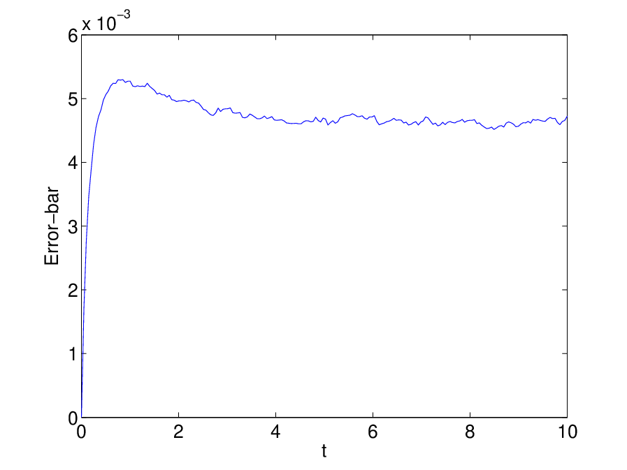
Given this estimated error, the calculated stochastic result for the correlation agrees with the exact solution within the sampling error.

VIII.3 Two-dimensional lattice calculation

As a non-trivial example calculation, we consider a $10\times 10$ Ising model with periodic boundary conditions. Couplings are nearest neighbor, on a rectangular lattice with $J_{ij}=1$ and $h=0$ .

The numerically calculated nearest-neighbour correlation function is given for six different inverse temperatures $\beta$ . Once the relevant stochastic averages have reached steady-state, they are time-averaged as well as stochastically-averaged to give the correlation functions.

The results are shown in Figure (3), along with a comparison to the known exact solution[30] in the limit of an infinite lattice. The critical inverse temperature in this case is $\beta_{c}\approx 0.44$ , as seen in the exact solution.

IX Summary

We have shown how to obtain a general phase-space representation with positive-definite diffusion, for multiple SU(2) and more general SU( $n$ ) quantum systems, with couplings obtained from the corresponding operator algebra. In the case of qubits or two-level systems, the appropriate operator algebra is the spin half SU(2) algebra. This allows some further simplifications in obtaining evolution equations.

The main application of these methods is to obtain stochastic methods for calculating either canonical ensembles or time-evolution of coupled atomic or spin systems. We have taken the exactly soluble Ising model as an example. The resulting stochastic equations were solved for correlation functions at finite temperature, and we found excellent agreement with known exact results. These techniques can also be applied to more complex n-level cases, with time-evolution and coupling to external reservoirs.

Acknowledgements.

Funding for this research was generously provided by the Australian Research Council Center of Excellence program.

References

[1] E. Schrödinger, Naturwissenschaften 14, 664, 1926.
[2] R. H. Dicke, Phys. Rev. 93, 99 (1954).
[3] J. M. Radcliffe, J. Phys. A 4, 313 (1971).
[4] F. T. Arecchi, E. Courtens, R. Gilmore, and H. Thomas, Phys. Rev. A 6, 2211 (1972).
[5] A. Perelomov, Commun. Math. Phys. 26, 222 (1972); K. Nemoto, J. Phys. A: Math. Gen. 33, 3493 (2000).
[6] L. M. Narducci, C. A. Coulter, and C. M. Bowden, Phys. Rev. A 9, 829 (1974).
[7] R. Gilmore, C. M. Bowden, and L. M. Narducci, Phys. Rev. A 12, 1019 (1975).
[8] B. Sriram Shastry, G. S. Agarwal, and I. Rama Rao, Pramana 11, 85 (1978).
[9] C. T. Lee, Phys. Rev. A 30, 3308 (1984).
[10] P. D. Drummond, Phys. Letts. A 106, 118 (1984).
[11] D. M. Gitman and A. L. Shelepin, J. Phys A 26, 313 (1993).
[12] E. P. Wigner, Phys. Rev. 40, 749 (1932).
[13] K. Husimi, Proc. Phys. Math. Soc. Jpn. 22, 264 (1940).
[14] R. J. Glauber, Phys. Rev. 131, 2766 (1963); E. C. G. Sudarshan, Phys. Rev. Lett. 10, 277 (1963).
[15] K. E. Cahill and R. J. Glauber, Phys. Rev. 177, 1882 (1969).
[16] G. S. Agarwal and E. Wolf, Phys. Rev. D 2 , 2161 (1970).
[17] S. Chaturvedi, P. D. Drummond, and D. F. Walls, J. Phys. A 10, L187-192 (1977).
[18] P. D. Drummond, C. W. Gardiner, J. Phys. A: Math. Gen. 13, 2353 (1980).
[19] C. W. Gardiner, Quantum Noise, (Springer-Verlag, Berlin, 1991).
[20] P. Deuar and P. D. Drummond, Phys. Rev. A 66, 033812 (2002).
[21] S. Chaturvedi, E. Ercolessi, G. Marmo, G. Morandi, N. Mukunda amd R. Simon, J. Phys A. 39 1405 (2006).
[22] A. M. Smith and C. W. Gardiner, Phys. Rev. A. 38, 4073 (1988).
[23] Y. Castin, and I. Carusotto, J. Phys. B 34, 4589 (2001).
[24] E. A. Kochetov, Phys. Rev. B 52, 4402 (1995).
[25] S. R. White, Phys. Rev. Lett. 69, 2863 (1992).
[26] G. Vidal, Phys. Rev. Lett. 91, 147902 (2003).
[27] F. Verstraete, D. Porras and J.I. Cirac, Phys. Rev. Lett. 93, 227205 (2004).
[28] E. Ising, Z. Phys. 31, 253 (1925).
[29] L.D. Landau, E.M. Lifshitz, Statistical physics (Pergamon Press, 1958).
[30] L. Onsager, Phys. Rev. 65, 117 (1944).
[31] R.J. Baxter, Exactly solved models in statistical mechanics , (Acad. Press, 1982), F.Y. Wu, Rev. Mod. Phys. 54, 235 (1982).
[32] M. E. Fisher, Rev. Mod. Phys. 46, 597 (1974).
[33] K. Binder and A.P. Young, Rev. Mod. Phys., 58, 801 (1986).
[34] D. Stauffer, A. Aharony, Introduction to percolation theory , (Taylor & Francis, 1992).
[35] D. Jaksch, C. Bruder, J. I. Cirac, C. W. Gardiner and P. Zoller, Phys. Rev. Lett. 81, 3108 (1998).
[36] K. G. Wilson, Phys. Rev. D 10, 2445 (1974); D. M. Ceperley, Rev. Mod. Phys. 67, 279 (1995).
[37] K. Binder ed, Monte Carlo methods in statistical physics , (Springer, Berlin, 1979).
[38] R.H. Swendsen and J. S. Wang, Phys. Rev. Lett. 58, 86 (1987).
[39] H.W.J. Blote, J.R. Heringa and E. Luijten, Computer Physics Communications 147, 58 (2002); H.W.J. Blote, J.R. Heringa and M.M. Tsypin, Physical Review E 62, 77 (2000); J.R. Heringa and H.W.J. Blote, Physical Review E 57, 4976 (1998).
[40] N. Metropolis, A. Rosenbluth, M. Rosenbluth, A. Teller and E. Teller, J. Chem. Phys. 21, 1087 (1953).
[41] M. Hamermesh, Group Theory (Addison-Wesley, 1962).
[42] P.D. Drummond, P. Deuar, and K.V. Kheruntsyan, Phys. Rev. Lett. 92, 040405 (2004).
[43] A. Gilchrist, C. W. Gardiner, and P. D. Drummond, Phys. Rev. A 55, 3014 (1997).
[44] G. R. Collecutt and P. D. Drummond, Comput. Phys. Commun. 142, 219-223 (2001).
[45] For example, see website www.xmds.org. At the time of writing, this makes available an automatic code generator known as XMDS using clustering (parallel) technology, available under a public license.

	$\displaystyle\frac{\partial}{\partial z}\left\\|z\right\rangle$	$\displaystyle=$	$\displaystyle\frac{\partial}{\partial r}\left\\|z\right\rangle=\frac{-i\partial}{\partial\phi}\left\\|z\right\rangle\,\,,$
	$\displaystyle\frac{\partial}{\partial z^{*}}\left\langle z\right\\|\,$	$\displaystyle=$	$\displaystyle\frac{\partial}{\partial r}\left\langle z\right\\|=\frac{i\partial}{\partial\phi}\left\langle z\right\\|\,\,.$		(42)

Qubit phase-space: SU(nn) coherent state P-representations