Pressure and interaction measure of the gluon plasma
Abstract
We explore the thermodynamics of the gluon plasma in SU(3) Yang-Mills theory emerging from the non-trivial spatial dynamics of valence gluons. The lattice data suggest that these gluons interact with each other linearly at large spatial separations. At high temperatures, valence gluons should reproduce the pressure of the non-interacting Stefan-Boltzmann plasma along with the leading perturbative correction. These properties of valence gluons can be modeled in terms of the integral over their trajectories. We calculate such a world-line integral analytically and obtain the pressure and the interaction measure of the gluon plasma. Additionally, we account for the contributions of stochastic background fields to these thermodynamic quantities. The results turn out to be in a good agreement with the corresponding lattice data. In particular, the lattice-simulated peak of the interaction measure near the deconfinement critical temperature is reproduced.
I Introduction
How strong are the interactions in the quark-gluon plasma? In connection with RHIC heavy-ion experiments, this question has been posed [1] to understand the low shear viscosity necessary for a hydrodynamic description of the early phase of a heavy-ion collision [2]. On the lattice, strong interactions in the QCD plasma up to temperatures about twice the deconfinement critical temperature are known from simulations of the interaction measure [3, 4]. Analytic models aiming at a description of these lattice data use both perturbative [5] and nonperturbative [6] techniques. In the present paper, we revisit this problem by analytically calculating the pressure and the interaction measure of the gluon plasma. The main nonperturbative dynamical input of our calculation is the spatial confinement of valence gluons and the Polyakov loop, which are known from lattice simulations [7] and [8], respectively. Following previous works [6, 9], we use the term "valence gluons" emphasizing their confining interactions at large spatial distances. At small distances, valence gluons become quasi-free. Accordingly, the spatial Wilson loop of a valence gluon obeys the area law at large distances and goes to unity at small distances. Additionally, we model small spatial Wilson loops in such a way as to reproduce the known leading perturbative contribution to the pressure of the gluon plasma [10]. We manage to analytically calculate the world-line integral representing the free energy of a valence gluon at any distances. Furthermore, we account for the interaction of spatial valence gluons with temporal background fields through the Polyakov loop [6], and for stochastic background fields, which provide spatial confinement of valence gluons. It turns out that our model is able to reproduce the lattice data on the pressure and the interaction measure of the gluon plasma rather well.
The world-line integral representing the one-loop free energy of a valence gluon [6, 11] can be reduced to the Euler-Heisenberg effective Lagrangian in an auxiliary Abelian field of a purely geometric origin. The weight factor associated with this field is constructed in such a way as to reproduce the Wilson loop in the original non-Abelian theory. We emphasize that we are not considering a YM theory in a constant Abelian-type background field 11 1 The reduction of the world-line integral we are performing in this paper is similar to the one used in Ref. [12] in order to calculate the condensates of a heavy quark through a tensor ansatz for the minimal area [13, 14].. Another related approach to incorporate nonperturbative contributions to the one-loop effective action [15] uses the two-point correlation function of gluonic field strengths provided by the stochastic vacuum model [16].
The paper is organized as follows. Section II is devoted to the calculation of the world-line integral for a valence gluon using a parametrization for the minimal area in terms of the contour of the spatial Wilson loop. In Section III, we numerically evaluate the pressure and the interaction measure of the gluon plasma. In Section IV, we summarize our approach and the main results of the paper. In Appendix A, we evaluate the contributions of stochastic background fields to the pressure and the interaction measure.
II The set-up for the free-energy density
Lattice simulations [7, 3] in the deconfinement phase () show that averages of large spatial Wilson loops still exhibit an area law. In SU(3) YM theory, the critical temperature is [3] (see e.g. Ref. [17] for a review). This "magnetic" or "spatial" confinement [18] of spatial Wilson-loop averages is the main established nonperturbative phenomenon in the quark-gluon plasma. It does not contradict the genuine deconfinement of a static quark-antiquark pair represented by averages of space-time Wilson loops at . We follow the strategy of Refs. [6, 11, 9] to model the spatial confinement of the valence gluons by stochastic background fields . With the ansatz , the Euclidean YM partition function at finite temperature has the following form:
Here , is the three-dimensional volume, is the QCD field-strength tensor, and the averaging over the background -fields is symbolized by the brackets . All the functional integrations imply periodic boundary conditions , . Performing Gaussian integration over the valence gluons, one obtains the gluon determinant:
| (1) |
with the covariant derivative . Equation (1) includes the color degrees of freedom of the valence gluons and their physical polarizations, . In the one-loop approximation for the -field, it can be simplified further:
| (2) |
The loop of fast field fluctuations receives infinitely many contributions of the slow -field. In Eq. (2), "Tr" includes the trace "tr" over color indices and the functional trace over space-time coordinates.
The free-energy density is defined by the standard formula
| (3) |
The interactions of valence gluons with the background fields can be calculated through the world-line method. Representing the trace of in terms of the Schwinger proper time as , one has [19]
| (4) |
Each world-line path has a center . The integration over the positions of the centers yields the factor on the left-hand side of Eq. (3). The vector-function , , in Eq. (4) characterizes the shape of the contour of the Wilson loop relative to the center . The integration goes over world-line paths obeying the periodic boundary conditions
| (5) |
Furthermore, the summation goes over the winding number with a factor of 2 accounting for the modes with . The zero-temperature part of the free-energy density corresponding to the zeroth winding mode, , has been subtracted [6, 20]. For simplicity, we use the standard approximation which neglects the gluon spin term. Equation (4) represents the main idea of our approach that the valence gluons, as high-energy fluctuations of the gluonic field, propagate in a low-energy stochastic background, which enters Eq. (4) in the form of the Wilson-loop average
| (6) |
We use the notation with . For brevity, we will call the average (6) just "the Wilson loop" 22 2 In our notation, the trace ”tr” is normalized by dividing over the trace of the unit matrix in the adjoint representation, equal to . Therefore, with this definition, ..
We will argue that the Wilson loop factorizes into a purely spatial Wilson loop and an averaged -th power of a time-like Polyakov loop:
| (7) |
with
| (8) |
and
In Eq. (7), we have rewritten the spatial Wilson loop through the non-Abelian Stokes’ theorem. We have suppressed for simplicity the Schwinger strings, which connect the point where the field-strength tensor is defined to a given reference point on an arbitrary surface encircled by the contour . The integration in Eq. (8) goes over the purely spatial part of that surface characterized by the differential elements . By using the cumulant expansion, one can express the Wilson loop in terms of the connected averages (cumulants) of chromo-magnetic and chromo-electric fields, and . Lattice data [21] suggest that the cumulant-expansion series can be truncated at the second term, since the amplitudes of higher terms are significantly smaller. A general Wilson-loop calculation leads to three correlation functions
| (9) |
Following the lattice data [21], we assume that the correlation function vanishes right after the deconfinement phase transition. This fact ensures deconfinement. The same lattice data also indicate that the amplitude of the mixed chromo-electric–chromo-magnetic correlation function is by an order of magnitude smaller than the amplitude of the chromo-magnetic–chromo-magnetic correlation function . This property leads to factorization, Eq. (7). After factorization, the world-line integral over becomes a one-dimensional world-line integral for a free particle. Carrying it out, one arrives at the following expression (cf. Ref. [9]):
| (10) |
The dynamics of the strongly interacting gluon plasma is now encoded in the Polyakov and spatial Wilson loop expectation values, which make the free energy nontrivial. An expectation value of the spatial Wilson loop depends on the area of the minimal surface defined by the spatial contour . At small spatial separations between valence gluons, , that corresponds to a non-interacting Stefan-Boltzmann plasma. At large separations, a nonperturbative linear interaction between valence gluons emerges from the spatial area law, . By "interaction" we mean the "potential" for the gluonic pair evolving in some spatial direction. The linear "potential" between valence gluons at large spatial separations can originate from their interaction with chromo-magnetic background fields .
Furthermore, we mimic the leading perturbative contribution to the pressure [10] by modeling perturbative interactions of valence gluons in terms of the spatial Wilson loop. The corresponding short-distance ansatz for the renormalized spatial Wilson loop reads
where is the length of the contour, and the prefactor is chosen in such a way that the leading -correction to the Stefan-Boltzmann pressure is reproduced correctly. We associate the -term in the pressure with perturbative interactions due to the massless-gluon exchange at short distances . These distances are smaller than and , where the gluon mass terms in the propagator become effective (cf. the recent paper [22]). First, by comparing our result for the pressure with the known perturbative one [10], we will determine the limiting value of the function at . This limiting value alone is not sufficient, and in the second step, we will parametrize the functional form of .
Our short-distance ansatz for the spatial Wilson loop can be unified with the spatial-area law to a single formula
| (11) |
For the short-distance part, we have estimated the length of the contour, , as of order . Note that, in this way, just one single equation (11) reproduces both the small- and the large-distance regimes of the Wilson loop. Indeed, the first term in the exponent, which describes perturbative interactions of valence gluons, dominates for sufficiently small areas, whereas the second term dominates for sufficiently large areas.
We implement now an ansatz for the minimal area , which is crucial for the subsequent calculation:
| (12) |
It parametrizes a parasol-shaped surface made of thin segments, as depicted in Fig. 1. Note that, since , the point where the segments merge is the origin. Thus, ansatz (12) automatically selects from all cone-shaped surfaces having as a boundary the one of the minimal area. We further approximate the integral in Eq. (12) as follows:
| (13) |
with
The left-hand side of Eq. (13), given by Eq. (12), can be larger than its right-hand side. This happens if, in the course of its evolution in the spatial directions, the valence gluon performs backward and/or non-planar motions. Should this happen, the vector product changes its direction, and the vector integral on the right-hand side of Eq. (13) receives mutually cancelling contributions. The non-backtracking approximation adopted in Eq. (13) is widely used in the context of minimal surfaces allowing analytic calculations of the associated world-line integrals (see e.g. [9, 12, 23]). We further proceed with calculating separately the perturbative part and the full free-energy density of the gluon plasma.

II.1 The perturbative contribution to the free-energy density
At , the Stefan-Boltzmann law along with the leading perturbative correction [10],
| (14) |
reproduces more than 95% of the lattice-simulated pressure of the gluon plasma [3]. Therefore, at such temperatures, one can retain only the first term in the exponent of Eq. (11), where should go to a constant with the increase of . We determine the value of by calculating the perturbative contribution to the free-energy density with our ansatz for a small Wilson loop,
| (15) |
and equating the result to the known expression, Eq. (14). The perturbative contribution to the free-energy density has the form
| (16) |
where we have used the leading-order perturbative result for the averaged Polyakov loop [26]
| (17) |
To calculate the world-line integral in Eq. (16), we disentangle the fourth root in the exponent of Eq. (15) by introducing two identical auxiliary integrations as follows:
We further use the Hubbard-Stratonovich trick
| (18) |
where , and is an auxiliary constant Abelian magnetic field. It yields
This expression, plugged into the world-line integral, Eq. (16), describes nothing but the proper-time evolution of a charged particle in the effective Abelian field , governed by the Lorentz force . The world-line integration, which is equivalent to the "summation" over all Landau levels, leads to the bosonic Euler-Heisenberg Lagrangian [19], namely
| (19) |
The -integration can be performed analytically. We further set and denote
suppressing for brevity the temperature dependence of . Rescaling , we obtain
| (20) |
To the leading order of the -expansion, , and one can use the value of the integral
to recover the Stefan-Boltzmann result:
| (21) |
The next term of the -expansion of Eq. (20) should correspond to the -term in Eq. (14). To derive it, we should approximate , that yields
The -integration in this formula can be performed analytically, so that we obtain
To the order , this formula recovers again the Stefan-Boltzmann free-energy density, Eq. (21). The -term of interest can be obtained by approximating the sum over winding modes by the first two terms:
This yields the desired free-energy density
| (22) |
which can be compared with the known result, Eq. (14). Comparing the -terms, and , we conclude that the approximation of the full sum over winding modes by the - and the -terms is indeed very good. Comparing the -terms, we finally obtain:
| (23) |
We set the function to this constant value at the highest temperature of achievable by the lattice simulations. With the decrease of temperature, perturbation theory becomes less and less applicable. We impose this fade of perturbation theory by the gradual nullification of the function . The full free-energy density, corresponding to the spatial Wilson loop (11), will be calculated in the next Subsection.
II.2 The full free-energy density
To calculate the world-line integral with the full Wilson loop, Eq. (11), we first transform in the exponent to by introducing an auxiliary integration as
where
. By introducing one more such integration, we further transform to :
We can now apply the Hubbard-Stratonovich trick, Eq. (18), and integrate over analytically. With the use of Eq. (13), this yields
| (24) |
The world-line integration can again be performed by using Eq. (19), that finally yields the full free-energy density
| (25) |
The remaining ordinary integrations over , , and will be performed numerically in the next Section.
III Numerical evaluation
We fix now the temperature dependences of various quantities entering the calculation. We adopt the perturbative two-loop running coupling at finite temperature [3]
| (26) |
and for the case under study. Furthermore, we assume the value [3].
At temperatures smaller than the temperature of dimensional reduction, , all dimensionful quantities can be approximated by their zero-temperature values [24]. We use the value , as suggested by the same lattice data [3]. The temperature-dependent string tension in the adjoint representation of interest reads
| (27) |
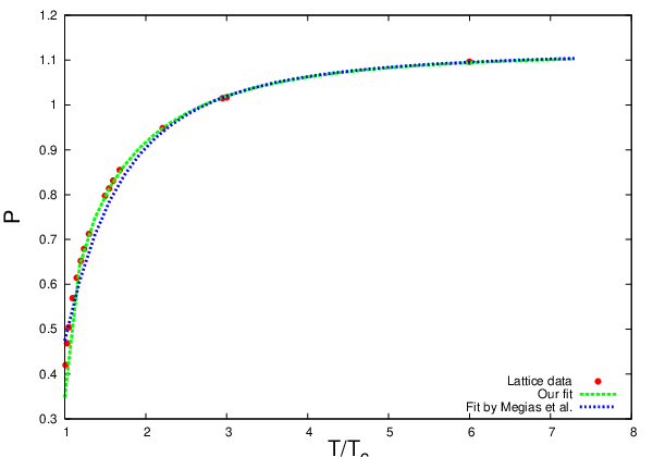
where is the zero-temperature value of the string tension in the fundamental representation. The coefficient 9/4 stems from the Casimir-scaling hypothesis for the string tensions in various representations. Casimir scaling has proven in Ref. [25] to be a good approximation also for the averaged Polyakov loop in the adjoint representation, . That is, this average can be approximated as , where is the averaged Polyakov loop in the fundamental representation, which has been simulated on the lattice in Ref. [8]. Since the - and -data from Ref. [8] follow the same pattern, we fit them both by the four-parameter function, which we use in the subsequent calculation:
| (28) |
In Fig. 2, we plot both the lattice data on the averaged Polyakov loop and the results of the fit. For comparison, in the same Fig. 2, we present the results of a simpler fit for the -data alone [27]
| (29) |
and observe a bit less good agreement. Note that, at , our fit for and the fit of Ref. [27] approach unity from above, in accordance with the positivity of the -correction in Eq. (17) [26, 22]. Furthermore, to estimate the effect of the second winding mode, we use for the averaged square of the Polyakov loop in the adjoint representation the following approximation: . Note that the freedom in choice of the renormalization scheme results in the multiplication of the renormalized Polyakov loop by a temperature-dependent factor. Such a multiplication is equivalent to the adding of some constant to the static quark-antiquark potential. We use here the values of the renormalized Polyakov loop in the fundamental representation from Ref. [8]. In that paper, is fixed to 0 by demanding the static potential at to have the form at , where the value of is given right after Eq. (27), and is the so-called Sommer scale [28]. Finally, to minimize the number of free parameters, we assume that the function rises linearly from 0 to the derived value (23) when grows from to , that is the maximal temperature at which the lattice values [3] for the pressure are available. Explicitly, the assumed function has the form
| (30) |
Using the above parametrizations, we calculate numerically the pressure of valence gluons
with their full free-energy density given by Eq. (25). This further yields their contribution to the interaction measure
Additionally, we take into account stochastic background fields, which provide spatial confinement of valence gluons in our model. Their contribution to the interaction measure is evaluated in Appendix A. We find that is nonvanishing and negative definite at temperatures , where its absolute value amounts to a few percent of .
In Fig. 3, we plot the full interaction measure
and compare it with the lattice results from Ref. [3]. In Fig. 4, we do the same for the full pressure,
Given all the approximations adopted, one can conclude that, for both the interaction measure and the pressure, the agreements with the corresponding lattice results are rather good.
Finally, one can define separately the perturbative and the nonperturbative contributions to the pressure. The perturbative contribution is given by Eq. (22) with the constant replaced by the full function given by Eq. (30). Explicitly, this contribution reads 33 3 Note that, at temperatures , the second term in this expression vanishes, and goes over to the Stefan-Boltzmann value approximated by the first two winding modes.
The nonperturbative contribution is accordingly defined as a difference
It includes the pressure produced by stochastic background fields and the nonperturbative part of the pressure produced by valence gluons. In Fig. 5, we plot , , and once again for comparison the lattice data on .


IV Summary and concluding remarks
The aim of the present paper has been an analytic calculation of the pressure and the interaction measure of the gluon plasma in SU(3) YM theory. Our main phenomenological input is confinement of valence gluons at large spatial separations and their perturbative interaction at small separations. The corresponding form of a spatial Wilson loop, Eq. (11), accounts for these interactions.
One can prove numerically that, at temperatures , the lattice-simulated pressure of the gluon plasma is by more than 95% described by the Stefan-Boltzmann law along with the perturbative interaction between valence gluons, Eq. (14). This fact enables us to fix the limiting high-temperature value of the function , which is used to parametrize the perturbative interaction in terms of spatial Wilson loops. The value of , Eq. (23), is obtained by analytically calculating the world-line integral with such a Wilson loop and comparing the obtained free-energy density with the known result (14).
At high temperatures, , valence gluons in our model interact both linearly at large spatial separations and Coulomb-like at small separations, while at only the large-distance linear part remains. With these interactions taken into account, we manage to analytically calculate the world-line integral, and obtain the contribution of spatial dynamics to the pressure at any temperature, Eq. (25). Additionally, we account also for the interaction of valence gluons with the -gluons via the Polyakov loop, which is taken as a fit to the lattice data [8, 25]. The critical behavior of the Polyakov loop is crucial for the nullification of the pressure at and a peak of the interaction measure near (cf. Refs. [6, 29]). Furthermore, stochastic background fields, that can be responsible for the spatial confinement of valence gluons, produce their own contributions to the interaction measure and the pressure, which are also taken into account [cf. Eqs. (33) and (34)]. In Figs. 3 and 4, we compare our results for these two thermodynamic quantities of the gluon plasma with the corresponding lattice data. The observed reasonable agreement suggests that spatially confined valence gluons, along with the stochastic background fields, could indeed be the right degrees of freedom for the description of the gluon-plasma thermodynamics.
Last but not least, we mention that, on the technical side, our paper advanced to analytically calculate the world-line integral with the minimal-area surface for each trajectory involved in the integration. Of course, it became possible only by virtue of a certain parametrization of such a surface in terms of the corresponding trajectory. Namely, we first assume that the surface has a parasol-shaped form, so that its area is , and use the approximation of non-backtracking planar trajectories . With the Hubbard-Stratonovich transformation (18), furthermore it is possible to single out the trajectory-dependence in the form , where is an auxiliary constant Abelian magnetic field. For such a field, the world-line integral becomes the known Euler-Heisenberg Lagrangian, Eq. (19). It looks promising to generalize this parametrization to the 4D case, that amounts to additionally introducing an effective Abelian electric field. Such an approach would enable one to systematically account for effects of confinement in various Feynman diagrams (cf. Ref. [9]). Work in this direction is in progress.
Finally, let us mention other recent studies, where the same thermodynamic quantities have been calculated either by analytic methods, perturbatively in [30] and nonperturbatively in [31], or on the lattice [32, 33]. In particular, Ref. [33] generalizing the interaction measure obtained in Ref. [3] to states that is approximately independent of for . This observation, once receiving confirmation by further lattice measurements, deserves theoretical interpretation.
Acknowledgements
We are grateful for usefuls discussions and correspondences to O. Andreev, J.-P. Blaizot, D. Grünewald, E.-M. Ilgenfritz, O. Kaczmarek, F. Karsch, M. Laine, E. Megias, M. Panero, and Yu.A. Simonov. We also thank F. Karsch and P. Petreczky for providing the details of the lattice data. The work of D.A. has been supported by the Helmholtz Alliance Program of the Helmholtz Association, contract HA-216 "Extremes of Density and Temperature: Cosmic Matter in the Laboratory", at the initial stage, and by the German Research Foundation (DFG), contract Sh 92/2-1, at the final stage.
Appendix A. Contributions of stochastic background fields to the pressure and the interaction measure
The contribution of stochastic background fields to the interaction measure can be calculated directly, by the known formula, which assumes no valence gluons [34]
| (31) |
with in the two-loop approximation adopted [cf. Eq. (26)], and . The contribution of the chromo-magnetic condensate to the trace anomaly in the vacuum is subtracted. It amounts to a half of the full contribution, while the other half is represented by the chromo-electric gluon condensate , whose “evaporation” at leads to deconfinement [11, 16, 21]. Thus, , where the value of the full condensate consistent with the known values of the string tension and of the vacuum correlation length [21] is [9, 35]. The temperature dependence of the chromo-magnetic condensate can be modeled by a formula similar to Eq. (27),
| (32) |
According to Eqs. (31) and (32), stochastic background fields alone produce no contribution to the interaction measure at , due to the constancy of at these temperatures 44 4 We disregard the exponentially small corrections to the constant values of and at , whose explicit form can be found in Ref. [24].. At , this contribution starts appearing, but at the highest temperature under consideration, , it must vanish again, as we assume that at this temperature all thermodynamic quantities are completely saturated by perturbative interactions of valence gluons. Since the increase of the perturbative contribution is given by the function (30), the simultaneous decrease of the nonperturbative contribution should be described by the function , where , Eq. (23). Hence, the contribution of stochastic background fields to the interaction measure can be parametrized as
| (33) |
The contribution to the pressure produced by stochastic background fields, , can be obtained by integrating the formula
from , below which , on. This contribution thus reads
| (34) |
As follows from Eqs. (32)-(34), both and are negative definite, leading to the decreases of the full and by a few percent at .
References
- [1] For reviews see e.g.: J. L. Nagle, Eur. Phys. J. C 49, 275 (2007); J. I. Kapusta, “Viscous properties of strongly interacting matter at high temperature,” arXiv:0809.3746 [nucl-th].
- [2] P. Romatschke and U. Romatschke, Phys. Rev. Lett. 99, 172301 (2007).
- [3] G. Boyd, J. Engels, F. Karsch, E. Lärmann, C. Legeland, M. Lütgemeier and B. Petersson, Nucl. Phys. B 469, 419 (1996).
- [4] M. Cheng et al., Phys. Rev. D 77, 014511 (2008).
- [5] J. P. Blaizot, E. Iancu and A. Rebhan, Phys. Rev. Lett. 83, 2906 (1999); Phys. Lett. B 470, 181 (1999); Phys. Rev. D 63, 065003 (2001).
- [6] H.G. Dosch, H.-J. Pirner and Yu.A. Simonov, Phys. Lett. B 349, 335 (1995).
- [7] G. S. Bali, J. Fingberg, U. M. Heller, F. Karsch and K. Schilling, Phys. Rev. Lett. 71, 3059 (1993).
- [8] O. Kaczmarek, F. Karsch, P. Petreczky and F. Zantow, Phys. Lett. B 543, 41 (2002).
- [9] D. Antonov and H. J. Pirner, Eur. Phys. J. C 51, 633 (2007).
- [10] E. V. Shuryak, Sov. Phys. JETP 47, 212 (1978).
- [11] Yu. A. Simonov, Phys. Atom. Nucl. 58, 309 (1995) [arXiv:hep-ph/9311216].
- [12] D. Antonov, JHEP 10, 030 (2003); ibid. 10, 018 (2005); Nucl. Phys. Proc. Suppl. 152, 144 (2006).
- [13] A. M. Polyakov, Nucl. Phys. B 164, 171 (1980).
- [14] M. A. Shifman, Nucl. Phys. B 173, 13 (1980); A. A. Migdal, Int. J. Mod. Phys. A 9, 1197 (1994).
- [15] S. J. Huber, A. Laser, M. Reuter and M. G. Schmidt, Nucl. Phys. B 539, 477 (1999); S. J. Huber, M. Reuter and M. G. Schmidt, Phys. Lett. B 462, 158 (1999).
- [16] For a review see: A. Di Giacomo, H. G. Dosch, V. I. Shevchenko and Yu. A. Simonov, Phys. Rept. 372, 319 (2002).
- [17] P. Petreczky, Eur. Phys. J. C 43, 51 (2005).
- [18] C. Borgs, Nucl. Phys. B 261, 455 (1985); E. Manousakis and J. Polonyi, Phys. Rev. Lett. 58, 847 (1987); Yu. A. Simonov, JETP Lett. 54, 249 (1991).
- [19] For reviews see: M. Reuter, M. G. Schmidt and C. Schubert, Annals Phys. 259, 313 (1997); C. Schubert, Phys. Rept. 355, 73 (2001); G. V. Dunne, “Heisenberg-Euler effective Lagrangians: Basics and extensions,” arXiv:hep-th/0406216.
- [20] B. J. Schäfer and H. J. Pirner, Nucl. Phys. A 627, 481 (1997).
- [21] A. Di Giacomo, E. Meggiolaro and H. Panagopoulos, Nucl. Phys. B 483, 371 (1997); M. D’Elia, A. Di Giacomo and E. Meggiolaro, Phys. Rev. D 67, 114504 (2003).
- [22] Y. Hidaka and R. D. Pisarski, “Zero point energy of renormalized Wilson loops,” arXiv:0907.4609 [hep-ph].
- [23] N. Brambilla, P. Consoli and G. M. Prosperi, Phys. Rev. D 50, 5878 (1994); A. Yu. Dubin, A. B. Kaidalov and Yu. A. Simonov, Phys. Lett. B 323, 41 (1994); Yu. Makeenko and P. Olesen, Phys. Rev. Lett. 102, 071602 (2009).
- [24] N. O. Agasian, Phys. Lett. B 562, 257 (2003).
- [25] S. Gupta, K. Hübner and O. Kaczmarek, Phys. Rev. D 77, 034503 (2008).
- [26] E. Gava and R. Jengo, Phys. Lett. B 105, 285 (1981).
- [27] E. Megias, E. Ruiz Arriola and L. L. Salcedo, JHEP 01, 073 (2006).
- [28] R. Sommer, Nucl. Phys. B 411, 839 (1994); S. Necco and R. Sommer, Phys. Lett. B 523, 135 (2001).
- [29] P. N. Meisinger, M. C. Ogilvie and T. R. Miller, Phys. Lett. B 585, 149 (2004).
- [30] A. Hietanen, K. Kajantie, M. Laine, K. Rummukainen and Y. Schröder, Phys. Rev. D 79, 045018 (2009).
- [31] E. V. Komarov and Yu. A. Simonov, Annals Phys. 323, 783 (2008), ibid. 323, 1230 (2008).
- [32] M. N. Chernodub, K. Ishiguro, A. Nakamura, T. Sekido, T. Suzuki and V. I. Zakharov, PoS LAT2007, 174 (2007).
- [33] M. Panero, “Geometric effects in lattice QCD thermodynamics,” arXiv:0808.1672 [hep-lat].
- [34] H. Leutwyler, in Proceedings of “QCD - 20 years later”, eds. P. M. Zerwas and H. A. Kastrup, World Scientific, 1993, p. 693.
- [35] A. I. Shoshi, F. D. Steffen, H. G. Dosch and H. J. Pirner, Phys. Rev. D 68, 074004 (2003).