跳到论文正文
W Papers独立论文阅读器 arXiv:0808.2154 论文正文 计算阅读时间 · 0%
引用这篇论文根据当前论文元数据生成,正式投稿前建议核对。


License: arXiv.org perpetual non-exclusive license
arXiv:0808.2154v1 [hep-ph] 15 Aug 2008

Wilson lines - color charge densities correlators and the production of η′\eta^{\prime} in the CGC for p​ppp and p​ApA collisions

François Fillion-Gourdeau Email: ffillion@hep.physics.mcgill.ca Affiliation: Department of Physics, McGill University, 3600 University Street, Montreal, Canada H3A 2T8    Sangyong Jeon Email: jeon@physics.mcgill.ca Affiliation: Department of Physics, McGill University, 3600 University Street, Montreal, Canada H3A 2T8
August 24, 2026
Abstract

We compute the inclusive differential cross section production of the pseudo-scalar meson η′\eta^{\prime} in high-energy proton-proton (p​ppp) and proton-nucleus (p​ApA) collisions. We use an effective coupling between gluons and η′\eta^{\prime} meson to derive a reduction formula that relates the η′\eta^{\prime} production to a field-strength tensor correlator. For p​ApA collisions we take into account saturation effects on the nucleus side by using the Color Glass Condensate formalism to evaluate this correlator. We derive new results for Wilson line - color charges correlators in the McLerran-Venugopalan model needed in the computation of η′\eta^{\prime} production. The unintegrated parton distribution functions are used to characterize the gluon distribution inside protons. We show that in p​ppp collisions, the cross section depends on the parametrization of unintegrated parton distribution functions and thus, it can be used to put constraints on these distributions. We also demonstrate that in p​ApA collisions, the cross section is sensitive to saturation effects so it can be utilized to estimate the value of the saturation scale.

I Introduction

One of the main challenges in high energy hadronic collisions is the understanding of particle production. The theoretical description of these complex phenomena involves both many-body physics and the theory of strong interactions. There are many approaches that aim toward a better comprehension of these topics. One of the most successful technique is perturbative quantum chromodynamics (pQCD) where one studies the limit where the coupling constant is small and where the usual loop expansion can be used in principle. Because QCD is an asymptotically free theory, this happens when the exchanged momenta are large compared to the QCD scale ΛQCD\Lambda_{\rm{QCD}}. Even in that regime however, physical observables computed using this machinery suffer from infrared divergences that spoil the naive perturbative expansion. These have to be resummed and this leads to various factorization formalisms like the collinear factorization and the k⟂k_{\perp}-factorization. In collinear factorization, meaningful physical quantities are obtained in terms of parton distribution functions (PDF). These distributions characterize the non-perturbative (large distance) physics and have to be determined experimentally from a fit to structure functions. This formalism can be applied on system where the typical exchanged momentum QQ is hard, which means that it satisfies the inequality given by ΛQCD2≪Q2∼s\Lambda_{\rm{QCD}}^{2}\ll Q^{2}\sim s where ΛQCD≈0.2​GeV\Lambda_{\rm{QCD}}\approx 0.2\;\mbox{GeV} is the QCD scale and s\sqrt{s} is the center of mass energy. Note that Q2∼M⟂2≡M2+k⟂2Q^{2}\sim M_{\perp}^{2}\equiv M^{2}+k_{\perp}^{2}, which means that unless the mass of the produced particle MM is of the order of s\sqrt{s}, the collinear factorization is valid only for very large k⟂k_{\perp}. This can be relaxed in the k⟂k_{\perp}-factorization formalism which considers semihard collisions, meaning that the typical exchanged momentum obeys ΛQCD2≪Q2≪s\Lambda_{\rm{QCD}}^{2}\ll Q^{2}\ll s. The resummation implemented in this approach takes care of large contributions that look like [ln⁡(Q2/ΛQ​C​D2)​αs]n\left[\ln(Q^{2}/\Lambda_{QCD}^{2})\alpha_{s}\right]^{n}, [ln⁡(Q2/ΛQ​C​D2)​ln⁡(1/x)​αs]n\left[\ln(Q^{2}/\Lambda_{QCD}^{2})\ln(1/x)\alpha_{s}\right]^{n} and [ln⁡(1/x)​αs]n\left[\ln(1/x)\alpha_{s}\right]^{n} [1, 2, 3, 4]. This technique is used successfully to compute the production of many kinds of particles in high energy proton-proton collisions like heavy quarks [1, 5, 6, 7, 8] and in a number of other processes (see [9, 10, 11] for reviews of many applications). It is also used for predictions of Higgs boson production [12, 13]. In this article, we use this formalism to compute the η′\eta^{\prime} inclusive cross section at the RHIC energy.

When there is a nucleus involved in a collision at very high energy, there are new effects not included in the previous approaches due to the high density of gluons resulting from the emission enhancement at small-xx (where xx is the momentum fraction). These effects introduce a new scale QsQ_{s} called the saturation scale at which the probability of having interactions between gluons of the same nucleus becomes important. At this transverse momentum scale, the gluons recombine and this slows down the growth of partons at smaller xx. A naive estimation of QsQ_{s} shows that it depends on xx and the number of nucleons AA like Qs2∼Aδ​x−λQ_{s}^{2}\sim A^{\delta}x^{-\lambda} [14, 15] so at small enough xx or large enough AA, the saturation scale is hard (Qs2≫ΛQCD2Q_{s}^{2}\gg\Lambda_{\rm{QCD}}^{2}). When the typical exchanged momentum is smaller than the saturation scale such as ΛQCD2≪Q2≤Qs2≪s\Lambda_{\rm{QCD}}^{2}\ll Q^{2}\leq Q_{s}^{2}\ll s, saturation effects have to be taken into account even if the system is still in the perturbative regime. This can be achieved in the Color Glass Condensate (CGC) formalism which is a semi-classical effective theory where the non-linearities are dealt with by solving exactly the Yang-Mills equation of motion. This takes care of gluon recombinations and introduces the effects of saturation in observables.

In this article, we are using the CGC to compute the inclusive differential cross section of η′\eta^{\prime} meson in p​ApA collisions at the RHIC energy (s=200​GeV\sqrt{s}=200\;\mbox{GeV}). The main goal of this work is to look at the effect of saturation in η′\eta^{\prime} production to validate the CGC approach and estimate the value of the saturation scale by comparing our predictions with experimental data. The η′\eta^{\prime} is a pseudoscalar meson with a mass of M=0.957​GeVM=0.957\;\mbox{GeV}, a decay width of 0.203​MeV0.203\;\mbox{MeV} and quantum numbers of IG​(JP​C)=0+​(0−⁣+)I^{G}(J^{PC})=0^{+}(0^{-+}) [16]. One of the most important features of η′\eta^{\prime} is that it couples to the QCD anomaly [17, 18]. One way to implement and model this physics is by introducing an effective interaction between gluons and η′\eta^{\prime} mesons. This was done in [19], where the authors are proposing a vertex that couples two gluons and a η′\eta^{\prime} meson (g​g​η′gg\eta^{\prime}) to explain B mesons decay (B→η′+XB\rightarrow\eta^{\prime}+X). This vertex contains a form factor that depends generally on gluons and η′\eta^{\prime} momenta and that can be related to the η′\eta^{\prime} wave-function. The structure of this vertex was investigated thoroughly using various techniques like the hard scattering and the running coupling approaches. [20, 21, 22, 23, 24, 25]. We use these results on the gluons-η′\eta^{\prime} coupling to study the η′\eta^{\prime} production mechanism based on gluon fusion.

The η′\eta^{\prime} production in p​ppp collisions at high energy was studied in [26] where the exclusive cross section for the diffractive process p+p→p+p+η′p+p\rightarrow p+p+\eta^{\prime} is computed. In our study, we focus on the inclusive production mechanism p+p→η′+Xp+p\rightarrow\eta^{\prime}+X which shares similar features with this previous analysis. The first attempt to compute η′\eta^{\prime} production in high energy p​ApA collisions was done by one of the present author in [27]. In this study, the collinear factorization is used to compute the cross section at RHIC by including intrinsic transverse momentum in the PDF with a Gaussian distribution. Based on physical arguments, the width of the Gaussian, which represents the typical transverse momentum of gluons inside the nucleus, is chosen to be QsQ_{s}. The authors show that the η′\eta^{\prime} production is sensitive to the saturation scale implemented in this way. However, they acknowledge that their calculation can be improved because they use the collinear formalism outside its range of validity. The goal of this article is to revisit the η′\eta^{\prime} production with a more rigorous approach by doing a full CGC computation that includes recombination effects more realistically.

The computation of meson production in the CGC was undertaken in the past using mostly an “hybrid” approach where the proton and the nucleus are described by the collinear factorization and the CGC respectively. In this formalism based on pQCD-like techniques, the fragmentation function of collinear factorization is convoluted with the gluon or quark cross section computed in the CGC formalism. This is suitable for well-known mesons like pions for which a wealth of experimental data have been measured and for which fragmentation functions are well-known. Pion production for p​ApA collisions is computed in [28, 29, 30] using this methodology. Contrary to pions, the data in high energy hadronic collisions for η′\eta^{\prime} is scarce, so another approach is required to take care of hadronization effects and internal structure of the η′\eta^{\prime} meson. In [31], an effective theory is used to estimate the tensor meson production in p​ppp collisions. We use a similar approach in this article where the interaction between gluons and η′\eta^{\prime} is described by an effective theory. As discussed previously, we include these effects in an effective vertex that includes a form factor. As will be shown in this article, this can be implemented easily in the CGC formalism.

We consider only the case of p​ppp and p​ApA collisions at RHIC. For nucleus-nucleus (A​AAA) collisions, the total number of η′\eta^{\prime}-mesons produced by semihard collisions in the first instants (for t<1​fm/ct<1\;\mbox{fm/c}) should be important and the saturation effects would also be present. Experimentally however, they cannot be detected because most of them decay inside the medium created by the collision. This is because the η′\eta^{\prime} mean lifetime, which is about tη′≈4.93​fm/ct_{\eta^{\prime}}\approx 4.93\;\mbox{fm/c}, is smaller than the time where the medium exists, which is from 1​fm/c1\;\mbox{fm/c} up to 10​fm/c10\;\mbox{fm/c}. Moreover, by considering p​ppp and p​ApA, we avoid all the complications that would result from the creation of the medium which include the understanding and modelling of the quark-gluon plasma properties. Finally, there are analytical solutions for the gauge field in p​ppp and p​ApA collisions, while the analytical solution in A​AAA is still elusive. For these reasons, our present analysis is only applied to p​ppp and p​ApA collisions.

This article is organized as follows. In section II we describe the effective vertex used throughout the rest of the article. In section III, we show how to compute η′\eta^{\prime} production in the CGC for p​ApA and p​ppp collisions. We start by deriving a reduction formula that relates the cross section to a correlator of field-strength tensors. This correlator is then evaluated to leading order in p​ApA collisions and the result can be interpreted in terms of physical processes. We also show how the k⟂k_{\perp}-factorized cross section for p​ppp collisions can be recovered in the low density limit of p​ApA cross section. In section IV, we compute the correlators appearing in the expression of the p​ApA cross section using the McLerran-Venugopalan model. In section V, we evaluate numerically the cross section for p​ApA and p​ppp and discuss the range of validity of our computation. Sections III and IV contain a lot of technical details. The reader interested in results can jump directly to section V.

Throughout the article, we use both light-cone coordinates defined by

p+\displaystyle p^{+} =\displaystyle= p0+p32;p−=p0−p32\displaystyle\frac{p^{0}+p^{3}}{\sqrt{2}}\;;\;p^{-}=\frac{p^{0}-p^{3}}{\sqrt{2}} (1)

and Minkowski coordinates. It should be clear by the context which one is used. We also use the metric convention gμ​ν=(1,−1,−1,−1)g_{\mu\nu}=(1,-1,-1,-1).

II Effective Theory

The effective theory used in this article couples gluons and the η′\eta^{\prime} meson. In momentum space, the g∗​g∗​η′g^{*}g^{*}\eta^{\prime} effective vertex (where g∗g^{*} means off-shell gluon) is given by

Vμ​ν​(M,p,q)=i​F​(p2,q2,M2)​δa​b​ϵμ​ν​ρ​α​pρ​qα\displaystyle V^{\mu\nu}(M,p,q)=iF(p^{2},q^{2},M^{2})\delta_{ab}\epsilon^{\mu\nu\rho\alpha}p_{\rho}q_{\alpha} (2)

where ϵμ​ν​ρ​α\epsilon^{\mu\nu\rho\alpha} is the Levi-Civitta antisymmetric tensor, MM is the η′\eta^{\prime} mass, aa and bb are color indices, pρp_{\rho} and qαq_{\alpha} are gluon momenta and F⁡(p2,q2,M2)F(p^{2},q^{2},M^{2}) is the η′\eta^{\prime} form factor. The explicit expression of the interaction vertex have been studied in a number of articles where different parametrizations of the form factor can be found [19, 20, 21, 22, 23, 24, 25]. To get a first approximation of η′\eta^{\prime} production and because we are mostly interested in making a comparative study between p​ppp and p​ApA collisions, we use a simple expression given by [26]

F⁡(p2,q2,M2)=H0​M4(M2−p2)​(M2−q2)\displaystyle F(p^{2},q^{2},M^{2})=H_{0}\frac{M^{4}}{(M^{2}-p^{2})(M^{2}-q^{2})} (3)

where H0=F⁡(0,0,M2)H_{0}=F(0,0,M^{2}). To get a better approximations of η′\eta^{\prime} production, other parametrizations should be used. In the limit of no gluon virtualities (p2,q2=0p^{2},q^{2}=0), the form factor is a constant that can be fixed by looking at the decay of ψ→η′+γ\psi\rightarrow\eta^{\prime}+\gamma. It is given by H0=F⁡(0,0,M2)≈1.8​GeVH_{0}=F(0,0,M^{2})\approx 1.8\;\mbox{GeV} [19].

The main applications of this coupling are related mostly to BB and Υ\Upsilon decay where processes such as g∗→g+η′g^{*}\rightarrow g+\eta^{\prime} and g∗+g∗→η′g^{*}+g^{*}\rightarrow\eta^{\prime} are considered [19, 32, 33, 34, 35]. More recently, gluon fusion was used to compute η′\eta^{\prime} production in high energy hadronic collisions [26, 27, 36] and from a thermalized medium [37].

It is convenient for our purpose to consider the interaction Lagrangian given by

ℒint​(x)=18​∫d4​y​d4​z​F​[(x−y)2,(x−z)2,M2]​Gaμ​ν​(y)​G~a,μ​ν​(z)​η​(x).\displaystyle\mathcal{L}_{\rm{int}}(x)=\frac{1}{8}\int d^{4}yd^{4}zF\left[(x-y)^{2},(x-z)^{2},M^{2}\right]G_{a}^{\mu\nu}(y)\widetilde{G}_{a,\mu\nu}(z)\eta(x). (4)

that reproduces the vertex Eq. (2) in the perturbative expansion. As seen in the next section, this can then be used to derive a reduction formula. Here, Gaμ​ν​(x)G_{a}^{\mu\nu}(x) is the usual field-strength tensor given by

Gaμ​ν​(x)=∂μAaν​(x)−∂νAaμ​(x)−g​fa​b​c​Abμ​(x)​Acν​(x)\displaystyle G_{a}^{\mu\nu}(x)=\partial^{\mu}A_{a}^{\nu}(x)-\partial^{\nu}A_{a}^{\mu}(x)-gf_{abc}A_{b}^{\mu}(x)A_{c}^{\nu}(x) (5)

where AaμA^{\mu}_{a} is the gauge field of gluons and G~aμ​ν​(x)=ϵμ​ν​ρ​σ​Ga,ρ​σ​(x)\tilde{G}_{a}^{\mu\nu}(x)=\epsilon^{\mu\nu\rho\sigma}G_{a,\rho\sigma}(x) is the dual field-strength tensor. The Lagrangian is non-local because the vertex includes a form factor. It can be easily seen that ℒint​(x)\mathcal{L}_{\rm{int}}(x) contains three types of vertices, namely g​g​η′gg\eta^{\prime}, g​g​g​η′ggg\eta^{\prime} and g​g​g​g​η′gggg\eta^{\prime}. At leading order however, only the first one is necessary and considered in this article.

III Production of η′\eta^{\prime} from the CGC

In collisions at very high energy, the wave function of nuclei is dominated by gluons that have small longitudinal momenta (soft gluons) because of the emission enhancement at small-xx. The CGC is a semi-classical formalism that describes the dynamics of these degrees of freedom. In this approach, the hard partons, which carry most of the longitudinal momentum, and soft gluons which have small longitudinal components, are treated differently. Because the occupation number of the soft gluons is large, classical field equations can be employed to understand their dynamics. The hard partons act as sources for these classical field and are no longer interacting with the rest of the system (for reviews of CGC, see [14, 15, 38]).

In this formalism, computing a physical quantity involves two main steps. The first one is to solve the Yang-Mills equation of motion

[Dμ,Fμ​ν​(x)]=Jν​(x)\displaystyle[D_{\mu},F^{\mu\nu}(x)]=J^{\nu}(x) (6)

where the current Jaν​(x)=δν+​δ​(x−)​ρp,a​(x⟂)+δν−​δ​(x+)​ρA,a​(x⟂)J^{\nu}_{a}(x)=\delta^{\nu+}\delta(x^{-})\rho_{p,a}(x_{\perp})+\delta^{\nu-}\delta(x^{+})\rho_{A,a}(x_{\perp}) represents random static sources localized on the light-cone [14, 15] and Dμ=∂μ−igAμD^{\mu}=\partial^{\mu}-igA^{\mu} is the covariant derivative. The functions ρp,A​(x⟂)\rho_{p,A}(x_{\perp}) are color charge densities in the transverse plane of the proton and nucleus respectively. The next step is to take the average over the distribution of color charge densities in the nuclei with weight functionals Wp,A​[ρp,A]W_{p,A}[\rho_{p,A}]. For any operator that can be related to color charge densities, this can be written as

⟨O^⟩=∫𝒟​ρp​𝒟​ρA​O​[ρp,ρA]​Wp​[xp,ρp]​WA​[xA,ρA].\displaystyle\langle\hat{O}\rangle=\int\mathcal{D}\rho_{p}\mathcal{D}\rho_{A}O[\rho_{p},\rho_{A}]W_{p}[x_{p},\rho_{p}]W_{A}[x_{A},\rho_{A}]. (7)

Computing the weight functional is a highly non-perturbative procedure so it usually involves approximations based on physical modelling. In the limit of a large nuclei at not too small xx, it can be approximated by the McLerran-Venugopalan (MV) model, which assumes that the partons are independent sources of color charge [39, 40]. Within this assumption, the weight functional WA​[ρA]W_{A}[\rho_{A}] is a xAx_{A} independent Gaussian distribution and the two point correlator is simply [39, 40, 14, 15]

⟨ρA,a​(x⟂)​ρA,b​(y⟂)⟩=δa​b​μA2​δ2​(x⟂−y⟂)\displaystyle\langle\rho_{A,a}(x_{\perp})\rho_{A,b}(y_{\perp})\rangle=\delta_{ab}\mu_{A}^{2}\delta^{2}(x_{\perp}-y_{\perp}) (8)

where μA2=A/2​π​R2\mu_{A}^{2}=A/2\pi R^{2} is the average color charge density and RR is the radius of the nucleus. It is assumed here that the nucleus has an infinite transverse extent with a constant charge distribution. Edge effects can be included by changing μ2→μ2​(x⟂)\mu^{2}\rightarrow\mu^{2}(x_{\perp}) and by choosing a suitable transverse profile. Throughout this article, we only consider the constant distribution case.

Within the MV model, the weight functional does not depend on longitudinal coordinates and therefore, the model is boost invariant. This however can be relaxed by considering the quantum version of the CGC. In that theory, quantum radiative corrections become important below a certain scale x0≈0.01x_{0}\approx 0.01. These corrections can be resummed by using a renormalization group technique which leads to the JIMWLK evolution equation [41, 42, 43, 44, 45]. In the quantum CGC, the weight functionals W1,2​[ρ1,2]W_{1,2}[\rho_{1,2}] obey this non-linear evolution equation in xx. Because the MV model is valid in the range x≈0.01−0.1x\approx 0.01-0.1, it can be used as an initial condition for the evolution at smaller xx. In this article however, we consider only the regime where the MV model is valid and do not consider the small-xx evolution although it could be done in principle.

On the proton side, the average computed with Wp​[xp,ρp]W_{p}[x_{p},\rho_{p}] can be related to the unintegrated parton distribution function (uPDF) ϕ1\phi_{1} like

g2​⟨ρp,a∗​(p⟂)​ρp,b​(q⟂)⟩\displaystyle g^{2}\langle\rho_{p,a}^{*}(p_{\perp})\rho_{p,b}(q_{\perp})\rangle =\displaystyle= 4​π2​δa​b(Nc2−1)​[p⟂+q⟂2]2\displaystyle\frac{4\pi^{2}\delta_{ab}}{(N^{2}_{c}-1)}\left[\frac{p_{\perp}+q_{\perp}}{2}\right]^{2} (9)
×∫d2​y⟂​ei⁡(p⟂−q⟂)⋅y⟂​d​ϕ1​(x,p⟂+q⟂2|y⟂)d2​y⟂\displaystyle\times\int d^{2}y_{\perp}e^{i(p_{\perp}-q_{\perp})\cdot y_{\perp}}\frac{d\phi_{1}\left(x,\frac{p_{\perp}+q_{\perp}}{2}|y_{\perp}\right)}{d^{2}y_{\perp}}

where NcN_{c} is the number of color. By construction, the uPDF obeys

∫d2​y⟂​d​ϕ1​(x,p⟂|y⟂)d2​y⟂=ϕ1​(x,p⟂)\displaystyle\int d^{2}y_{\perp}\frac{d\phi_{1}\left(x,p_{\perp}|y_{\perp}\right)}{d^{2}y_{\perp}}=\phi_{1}(x,p_{\perp}) (10)

and is normalized such that

∫0μ2ϕ1,2​(x,p⟂)≈x​G​(x,μ2)\displaystyle\int_{0}^{\mu^{2}}\phi_{1,2}(x,p_{\perp})\approx xG(x,\mu^{2}) (11)

where x​G​(x,μ2)xG(x,\mu^{2}) is the collinear parton distribution function and μ2\mu^{2} is the factorization scale. The uPDF can be obtained from a fit to structure function and evolved to the desired value of xpx_{p}, Q2Q^{2} and p⟂2p_{\perp}^{2} using evolution equations such as the BFKL or the CCFM equations.

One important ingredient is missing for the computation of η′\eta^{\prime} meson production cross section. We need a relation between the cross section and a correlator that can be evaluated using the CGC formalism. This is done in the next section using a reduction formula and the effective theory.

III.1 Reduction Formula and the Cross Section

The computation of η′\eta^{\prime} mesons from the CGC can be calculated from a reduction formula. The starting point is the expression of the average number of η′\eta^{\prime} produced per collisions given by n¯=∑n=1∞n​Pn\bar{n}=\sum_{n=1}^{\infty}nP_{n} where PnP_{n} is the probability to produce nn particles. This can be converted to an equation in terms of creation/annihilation operators that can be evaluated in quantum field theory. This is given by [46]

(2π)32Ekd​n¯d3​k=⟨0in|a^out†(k)a^out(k)|0in⟩\displaystyle(2\pi)^{3}2E_{k}\frac{d\bar{n}}{d^{3}k}=\left\langle 0_{\rm in}\right|\hat{a}^{\dagger}_{\rm out}(k)\hat{a}_{\rm out}(k)\left|0_{\rm in}\right\rangle (12)

where |0in⟩\left|0_{\rm in}\right\rangle is the in vacuum. Then, the standard LSZ procedure can be used to write this as [47]

(2π)32Ekd​n¯d3​k=1𝒵∫d4xd4yei​k⋅(x−y)[∂x2+M2][∂y2+M2]⟨0in|η^(x)η^(y)|0in⟩\displaystyle(2\pi)^{3}2E_{k}\frac{d\bar{n}}{d^{3}k}=\frac{1}{\mathcal{Z}}\int d^{4}xd^{4}ye^{ik\cdot(x-y)}\left[\partial_{x}^{2}+M^{2}\right]\left[\partial_{y}^{2}+M^{2}\right]\left\langle 0_{\rm in}\right|\hat{\eta}(x)\hat{\eta}(y)\left|0_{\rm in}\right\rangle (13)

where 𝒵\mathcal{Z} is the wave function normalization and where we assumed the asymptotic conditions limt→±∞η^​(x)=𝒵​η^out,in​(x)\lim_{t\rightarrow\pm\infty}\hat{\eta}(x)=\sqrt{\mathcal{Z}}\hat{\eta}_{\rm{out,in}}(x) for the η′\eta^{\prime} field operator in Heisenberg representation. It is possible to use the equation of motion of η^​(x)\hat{\eta}(x) given simply by

(∂2+M2)η^(x)\displaystyle(\partial^{2}+M^{2})\hat{\eta}(x) =\displaystyle= T^​(x)\displaystyle\hat{T}(x) (14)

where we defined T^​(x)≡18​∫d4​y​d4​z​F​[(x−y)2,(x−z)2,M2]​G^aμ​ν​(y)​G~^a,μ​ν​(z)\hat{T}(x)\equiv\frac{1}{8}\int d^{4}yd^{4}zF\left[(x-y)^{2},(x-z)^{2},M^{2}\right]\hat{G}_{a}^{\mu\nu}(y)\hat{\widetilde{G}}_{a,\mu\nu}(z) to rewrite the reduction formula in a convenient way. We get finally that

(2​π)3​2​Ek​d​n¯d3​k=⟨T^†​(k)​T^​(k)⟩\displaystyle(2\pi)^{3}2E_{k}\frac{d\bar{n}}{d^{3}k}=\langle\hat{T}^{\dagger}(k)\hat{T}(k)\rangle (15)

where T^​(k)\hat{T}(k) is the Fourier transform of T^​(x)\hat{T}(x) evaluated at a η′\eta^{\prime} meson on-shell momentum and where we set 𝒵=1\mathcal{Z}=1. The angular brackets ⟨O^⟩\langle\hat{O}\rangle here indicates expectation value of O^\hat{O} in the initial state.

The only assumptions used in deriving Eq. (15) are:

  • •

    There are no η′\eta^{\prime} mesons in the initial state.

  • •

    The η′\eta^{\prime} is produced on-shell.

The first assumption is justified by the fact that in high-energy collisions, the number of η′\eta^{\prime} in a hadron before the collision (in the initial state) is negligible. This allows us to use the in vacuum and the fact that ain​(k)​|0in⟩=0a_{\rm in}(k)|0_{\rm in}\rangle=0 to simplify the reduction formula. Using the second assumption, we can treat the η′\eta^{\prime} meson as a stable particle which can be produced on-shell and which is well described by the free spectral density that looks like ρ⁡(M2)∼δ⁡(p2−M2)\rho(M^{2})\sim\delta(p^{2}-M^{2}). Therefore, by making this assumption, it is possible to use the asymptotic conditions described earlier. However, η′\eta^{\prime}-mesons are resonances, so the spectral density should look rather as a Breit-Wigner function ρ⁡(M2)∼Γ/[(p2−M2)2+M2​Γ2]\rho(M^{2})\sim\Gamma/[(p^{2}-M^{2})^{2}+M^{2}\Gamma^{2}] where Γ\Gamma is the decay width. These effects however are taken into account by the form factor F⁡(q,p,M)F(q,p,M).

Eq. (15) is the main result of this section. It relates the average number of η′\eta^{\prime} mesons produced to a correlator of field strength tensors. This correlator can then be evaluated using any analytical or numerical methods. The average ⟨…⟩\langle...\rangle depends on the system studied. Looking at a plasma at equilibrium, it could be computed using finite temperature field theory or the AdS/CFT correspondence. These two formalisms are relevant to nucleus-nucleus collisions where a medium at equilibrium is created. We are interested here in p​ApA and p​ppp collisions where no such medium is formed so these techniques are not pursued in this study. Rather, we use the CGC which describes initial state and saturation effects in high-energy hadronic collisions.

Having expressed the average number of η′\eta^{\prime} produced in terms of a correlator of field strength tensors, it is possible to compute the inclusive cross section in the CGC formalism which is given by [48, 46]

(2​π)3​2​Ek​d​σd3​k\displaystyle(2\pi)^{3}2E_{k}\frac{d\sigma}{d^{3}k} =\displaystyle= ∫d2​b⟂​(2​π)3​2​Ek​d​n¯​(b⟂)d3​k\displaystyle\int d^{2}b_{\perp}(2\pi)^{3}2E_{k}\frac{d\bar{n}(b_{\perp})}{d^{3}k} (16)
=\displaystyle= ∫d2​b⟂​∫𝒟​ρp​𝒟​ρA​T∗​[ρp,ρA]​T​[ρp,ρA]\displaystyle\int d^{2}b_{\perp}\int\mathcal{D}\rho_{p}\mathcal{D}\rho_{A}T^{*}[\rho_{p},\rho_{A}]T[\rho_{p},\rho_{A}]
×Wp​[xp,ρp]​WA​[ρA;b⟂].\displaystyle\times W_{p}[x_{p},\rho_{p}]W_{A}[\rho_{A};b_{\perp}].

In this expression, b⟂b_{\perp} is the impact parameter. The fields TT are functionals of the source once the Yang-Mills equation of motion of the gauge field is solved (see Eq. (5) for the expression of the field strength tensor as a function of the gauge field).

III.2 Cross section in p​ApA Collisions

In p​ApA collisions, there are two saturation scales (one for the proton (QpQ_{p}) and one for the nucleus (QAQ_{A})) that satisfy Qp<QAQ_{p}<Q_{A}. When the transverse momentum of the η′\eta^{\prime} is small enough, the nucleus is in a saturation state while the proton is not because we have Qp2<Q2=M⟂2<QA2Q_{p}^{2}<Q^{2}=M_{\perp}^{2}<Q_{A}^{2} (remember that M⟂2=M2+k⟂2M_{\perp}^{2}=M^{2}+k_{\perp}^{2} is the transverse mass of the η′\eta^{\prime}). In that case, the system is semi-dilute, meaning that one of the source is strong (or equivalently, the typical transverse momentum is small) and obeys ρA,a​(k⟂)/k⟂2∼1\rho_{A,a}(k_{\perp})/k_{\perp}^{2}\sim 1 while the other source is still weak ρp,a​(k⟂)/k⟂2≪1\rho_{p,a}(k_{\perp})/k_{\perp}^{2}\ll 1 [38, 49]. The weak source can be used as a small parameter to solve the Yang-Mills equation perturbatively. The solution of the gauge field can be computed analytically to all orders in ρA,a​(k⟂)/k⟂2\rho_{A,a}(k_{\perp})/k_{\perp}^{2} and to first order in ρp,a​(k⟂)/k⟂2\rho_{p,a}(k_{\perp})/k_{\perp}^{2} in different gauges [50, 51, 52, 53]. We use here the solution in the light-cone gauge of the proton [52] but in Appendix C, we perform the same calculation in covariant gauge to show that our result is gauge invariant.

III.2.1 Gauge Field and Power Counting

In the light-cone gauge of the proton (A+=0A^{+}=0) with a nucleus in covariant gauge moving in the negative zz direction, the solution of the gauge field in p​ApA collisions can be separated in three parts Aaμ​(k)=Ap,aμ​(k)+AA,aμ​(k)+Ap​A,aμA^{\mu}_{a}(k)=A^{\mu}_{p,a}(k)+A^{\mu}_{A,a}(k)+A^{\mu}_{pA,a} where Ap,aμ​(k)A^{\mu}_{p,a}(k) is the field associated with the proton (of O⁡(ρp)O(\rho_{p})), AA,aμ​(k)A^{\mu}_{A,a}(k) is the field associated with the nuclei (of O⁡(ρA)∼O⁡(1)O(\rho_{A})\sim O(1)) and Ap​A,aμ​(k)A^{\mu}_{pA,a}(k) is the field produced by the collision (of O⁡(ρp​ρA∞)∼O⁡(ρp)O(\rho_{p}\rho_{A}^{\infty})\sim O(\rho_{p})) [52]. Note that the field AAμA^{\mu}_{A} is strong and satisfies Apμ,Ap​Aμ≪AAμA^{\mu}_{p},A^{\mu}_{pA}\ll A^{\mu}_{A}. The explicit solution is given by [52, 54]

Ap,ai​(k)\displaystyle A^{i}_{p,a}(k) =\displaystyle= 2​π​g​δ​(k−)​kik++i​ϵ​ρp,a​(k⟂)k⟂2\displaystyle 2\pi g\delta(k^{-})\frac{k^{i}}{k^{+}+i\epsilon}\frac{\rho_{p,a}(k_{\perp})}{k_{\perp}^{2}} (17)
AA,a−​(k)\displaystyle A^{-}_{A,a}(k) =\displaystyle= 2​π​g​δ​(k+)​ρA,a​(k⟂)k⟂2\displaystyle 2\pi g\delta(k^{+})\frac{\rho_{A,a}(k_{\perp})}{k_{\perp}^{2}} (18)
Ap​A,ai​(k)\displaystyle A^{i}_{pA,a}(k) =\displaystyle= −i​gk2+i​k+​ϵ∫d2​p⟂(2​π)2[ki(k++i​ϵ)​(k−+i​ϵ)−2pip⟂2]ρp,b(p⟂)\displaystyle-\frac{ig}{k^{2}+ik^{+}\epsilon}\int\frac{d^{2}p_{\perp}}{(2\pi)^{2}}\left[\frac{k^{i}}{(k^{+}+i\epsilon)(k^{-}+i\epsilon)}-2\frac{p^{i}}{p_{\perp}^{2}}\right]\rho_{p,b}(p_{\perp}) (19)
×[Ua​b​(k⟂−p⟂)−(2​π)2​δ2​(k⟂−p⟂)​δa​b]\displaystyle\times\left[U_{ab}(k_{\perp}-p_{\perp})-(2\pi)^{2}\delta^{2}(k_{\perp}-p_{\perp})\delta_{ab}\right]

where Ua​b​(k⟂)U_{ab}(k_{\perp}) is a Wilson line in adjoint representation defined in Eq. (35), gg is the usual QCD coupling constant, δa​b\delta_{ab} is the Kronecker delta in color space and fa​b​cf_{abc} is the structure constant of the S​U​(Nc)SU(N_{c}) group. The component Ap​A,a−​(k)A^{-}_{pA,a}(k) is non-zero and is related to Ap​A,ai​(k)A^{i}_{pA,a}(k) but it does not appear in the final expression of the cross section so it is not needed in the computation of η′\eta^{\prime} production. All the other components are zero.

The production cross section of η′\eta^{\prime} mesons is related to a field strength tensor correlator given by

B⁡(k)\displaystyle B(k) ≡\displaystyle\equiv ∫d4​p​d4​q(2​π)8​F​(p2,p22)​F∗​(q2,q22)​⟨Gμ​ν​a∗​(p)​G~a∗μ​ν​(k−p)​Gα​β​b​(q)​G~bα​β​(k−q)⟩\displaystyle\int\frac{d^{4}pd^{4}q}{(2\pi)^{8}}F(p^{2},p_{2}^{2})F^{*}(q^{2},q_{2}^{2})\langle G_{\mu\nu a}^{*}(p)\widetilde{G}^{*\mu\nu}_{a}(k-p)G_{\alpha\beta b}(q)\widetilde{G}^{\alpha\beta}_{b}(k-q)\rangle (20)

where p2,q2=k−p,qp_{2},q_{2}=k-p,q. In principle, a correlator like this contains contributions from all orders in both sources. Because the proton source is weak, it is possible to simplify this considerably using a power counting argument to isolate the leading order contribution. For the sake of this power counting argument, we use a(…)na_{(...)}^{n} which denotes terms having nn gauge fields A(…)μA_{(...)}^{\mu} and where aA∼O⁡(ρA)a_{A}\sim O(\rho_{A}) and ap,ap​A∼O⁡(ρp)a_{p},a_{pA}\sim O(\rho_{p}). At first, let us consider only the contributions from the abelian part of the field-strength tensor. The terms in these contributions have four powers of gauge field such as Babelian∼atot4∼(aA+ap+ap​A)4B_{\rm{abelian}}\sim a_{\rm{tot}}^{4}\sim(a_{A}+a_{p}+a_{pA})^{4}. Naively, one would expect the dominant contribution to come from terms that have many powers of the nucleus gauge field like aA4∼O⁡(ρA4)a_{A}^{4}\sim O(\rho^{4}_{A}) and aA3​ap,aA3​ap​A∼O⁡(ρA3​ρp)a_{A}^{3}a_{p},a_{A}^{3}a_{pA}\sim O(\rho^{3}_{A}\rho_{p}). However, these terms vanish because of the Lorentz structure. For example, a typical term in the abelian contribution would look like Tabelian∼ϵμ​ν​ρ​σ​pμ​qν​Aρ​AσT_{\mathrm{abelian}}\sim\epsilon_{\mu\nu\rho\sigma}p^{\mu}q^{\nu}A^{\rho}A^{\sigma}. When we sum on indices, this kind of term will contain at most one strong gauge field A−∼aAA^{-}\sim a_{A}. Thus, the dominant contributions are like aA2​ap2,aA2​ap​A2∼O⁡(ρA2​ρp2)a_{A}^{2}a_{p}^{2},a_{A}^{2}a_{pA}^{2}\sim O(\rho^{2}_{A}\rho^{2}_{p}). Using a similar argument, it is possible to show that the non-abelian part have no leading order contribution in the sense that it is at least Bnon−abelian∼O⁡(ρA2​ρp3)≪O⁡(ρA2​ρp2)B_{\rm{non-abelian}}\sim O(\rho^{2}_{A}\rho^{3}_{p})\ll O(\rho^{2}_{A}\rho^{2}_{p}). The possible higher order contributions like aA3​ap2∼O⁡(ρA3​ρp2)a_{A}^{3}a_{p}^{2}\sim O(\rho^{3}_{A}\rho^{2}_{p}) for example also vanish because of the Lorentz structure of the correlator. This is because the typical non-abelian contributions look like Tnon−abelian′∼ϵμ​ν​ρ​σ​pμ​Aν​Aρ​AσT^{\prime}_{\mathrm{non-abelian}}\sim\epsilon_{\mu\nu\rho\sigma}p^{\mu}A^{\nu}A^{\rho}A^{\sigma} and Tnon−abelian′′∼ϵμ​ν​ρ​σ​Aμ​Aν​Aρ​AσT^{\prime\prime}_{\mathrm{non-abelian}}\sim\epsilon_{\mu\nu\rho\sigma}A^{\mu}A^{\nu}A^{\rho}A^{\sigma}. Once the Lorentz indices are summed, the second typical term T′′=0T^{\prime\prime}=0 because in this gauge, A+=0A^{+}=0. For T′T^{\prime}, it contains only one strong field A−∼ap​AA^{-}\sim a_{pA} but it contains two powers of weak field like Ai∼ap,ap​AA^{i}\sim a_{p},a_{pA}. Thus, when it is squared, it gives at most a contribution of Bnon−abelian∼O⁡(ρA2​ρp3)B_{\rm{non-abelian}}\sim O(\rho^{2}_{A}\rho^{3}_{p}).

III.3 Evaluation of the Correlator

Using the explicit expression of the field strength tensor in terms of gauge field and keeping only the dominant and non-zero contributions, the correlator can be written as

B⁡(k)\displaystyle B(k) =\displaystyle= 64​∫d4​p​d4​q(2​π)8​F​(−p⟂2,−p2,⟂2)​F∗​(−q⟂2,−q2,⟂2)​(k+−p+)​(k+−q+)​ϵi​j​ϵk​l​pi​qk\displaystyle 64\int\frac{d^{4}pd^{4}q}{(2\pi)^{8}}F(-p_{\perp}^{2},-p_{2,\perp}^{2})F^{*}(-q_{\perp}^{2},-q_{2,\perp}^{2})(k^{+}-p^{+})(k^{+}-q^{+})\epsilon_{ij}\epsilon_{kl}p^{i}q^{k} (21)
×⟨AA,a−⁣∗(p)AA,b−(q)As,aj∗(k−p)As,bl(k−q)⟩\displaystyle\times\langle A_{A,a}^{-*}(p)A_{A,b}^{-}(q)A_{s,a}^{j*}(k-p)A_{s,b}^{l}(k-q)\rangle

where ϵi​j\epsilon_{ij} is the Levi-Civitta antisymmetric tensor with i,j=1,2i,j=1,2 and where we defined As,a≡Ap,a+Ap​A,aA_{s,a}\equiv A_{p,a}+A_{pA,a}.

To obtain the preceding expression we make the assumption that the virtualities in the form factors are due solely to transverse momentum such as F⁡(p2,p22)=F⁡(−p⟂2,−p2,⟂2)F(p^{2},p_{2}^{2})=F(-p_{\perp}^{2},-p_{2,\perp}^{2}). This approximation is necessary to recover k⟂k_{\perp}-factorization in the dilute limit as seen in section III.5.

It is convenient to separate B⁡(k)B(k) in four different terms such as

Bz,z′​(k)\displaystyle B_{z,z^{\prime}}(k) =\displaystyle= 64​g2​(k+)2​∫d​p−​d​q−​d2​p⟂​d2​q⟂(2​π)6​F​(−p⟂2,−p2,⟂2)​F∗​(−q⟂2,−q2,⟂2)​ϵi​j​ϵk​l​pi​qkp⟂2​q⟂2\displaystyle 64g^{2}(k^{+})^{2}\int\frac{dp^{-}dq^{-}d^{2}p_{\perp}d^{2}q_{\perp}}{(2\pi)^{6}}F(-p_{\perp}^{2},-p_{2,\perp}^{2})F^{*}(-q_{\perp}^{2},-q_{2,\perp}^{2})\epsilon_{ij}\epsilon_{kl}\frac{p^{i}q^{k}}{p^{2}_{\perp}q^{2}_{\perp}} (22)
×⟨ρA,a∗(p⟂)ρA,b(q⟂)Az,aj∗(k−p)Az′,bl(k−q)⟩|p+=q+=0\displaystyle\times\left.\langle\rho_{A,a}^{*}(p_{\perp})\rho_{A,b}(q_{\perp})A_{z,a}^{j*}(k-p)A_{z^{\prime},b}^{l}(k-q)\rangle\right|_{p^{+}=q^{+}=0}

where z,z′={p,p​A}z,z^{\prime}=\{p,pA\} and where we performed the integration on p+p^{+} and q+q^{+} using the delta functions in Eq. (18). These four terms can be evaluated explicitly by substituting the solution of gauge fields Eqs. (17), (18) and (19).

For the first term, it is a straightforward calculation to show that

Bp,p​(k)\displaystyle B_{p,p}(k) =\displaystyle= 64​g4​∫d2​p⟂​d2​q⟂​d2​r⟂​d2​s⟂(2​π)8​F​(−p⟂2,−p2,⟂2)​F∗​(−q⟂2,−q2,⟂2)\displaystyle 64g^{4}\int\frac{d^{2}p_{\perp}d^{2}q_{\perp}d^{2}r_{\perp}d^{2}s_{\perp}}{(2\pi)^{8}}F(-p_{\perp}^{2},-p_{2,\perp}^{2})F^{*}(-q_{\perp}^{2},-q_{2,\perp}^{2}) (23)
×ϵi​j​ϵk​l​pi​rj​qk​slp⟂2​q⟂2​r⟂2​s⟂2​δb​c​(2​π)2​δ2​(k⟂−p⟂−r⟂)​δa​d​(2​π)2​δ2​(k⟂−q⟂−s⟂)\displaystyle\times\epsilon_{ij}\epsilon_{kl}\frac{p^{i}r^{j}q^{k}s^{l}}{p^{2}_{\perp}q^{2}_{\perp}r^{2}_{\perp}s^{2}_{\perp}}\delta_{bc}(2\pi)^{2}\delta^{2}(k_{\perp}-p_{\perp}-r_{\perp})\delta_{ad}(2\pi)^{2}\delta^{2}(k_{\perp}-q_{\perp}-s_{\perp})
×⟨ρp,d∗​(r⟂)​ρp,c​(s⟂)⟩​⟨ρA,a∗​(p⟂)​ρA,b​(q⟂)⟩.\displaystyle\times\langle\rho_{p,d}^{*}(r_{\perp})\rho_{p,c}(s_{\perp})\rangle\langle\rho_{A,a}^{*}(p_{\perp})\rho_{A,b}(q_{\perp})\rangle.

The calculation of the second term is similar but requires some more work. By direct substitution of the expression of the gauge fields, we have

Bp​A,p​(k)\displaystyle B_{pA,p}(k) =\displaystyle= 64​i​g4​(k+)​∫d​p−​d2​p⟂​d2​q⟂​d2​r⟂(2​π)7​F​(−p⟂2,−p2,⟂2)​F∗​(−q⟂2,−q2,⟂2)\displaystyle 64ig^{4}(k^{+})\int\frac{dp^{-}d^{2}p_{\perp}d^{2}q_{\perp}d^{2}r_{\perp}}{(2\pi)^{7}}F(-p_{\perp}^{2},-p_{2,\perp}^{2})F^{*}(-q_{\perp}^{2},-q_{2,\perp}^{2}) (24)
×ϵi​j​ϵk​l​pi​qk​q2lp⟂2​q⟂2​q2,⟂2​1p22−i​k+​ϵ​[p2j(p2+−i​ϵ)​(p2−−i​ϵ)−2​rjr⟂2]\displaystyle\times\epsilon_{ij}\epsilon_{kl}\frac{p^{i}q^{k}q_{2}^{l}}{p^{2}_{\perp}q^{2}_{\perp}q_{2,\perp}^{2}}\frac{1}{p_{2}^{2}-ik^{+}\epsilon}\left[\frac{p_{2}^{j}}{(p_{2}^{+}-i\epsilon)(p_{2}^{-}-i\epsilon)}-2\frac{r^{j}}{r_{\perp}^{2}}\right]
×[⟨ρA,a∗(p⟂)ρA,b(q⟂)Ua​c∗(p2,⟂−r⟂)⟩⟨ρp,c∗(r⟂)ρp,b(q2,⟂)⟩\displaystyle\times\biggl[\langle\rho_{A,a}^{*}(p_{\perp})\rho_{A,b}(q_{\perp})U^{*}_{ac}(p_{2,\perp}-r_{\perp})\rangle\langle\rho_{p,c}^{*}(r_{\perp})\rho_{p,b}(q_{2,\perp})\rangle
−(2π)2δ2(p2,⟂−r⟂)δa​c⟨ρA,a∗(p⟂)ρA,b(q⟂)⟩⟨ρp,c∗(r⟂)ρp,b(q2,⟂)⟩].\displaystyle-(2\pi)^{2}\delta^{2}(p_{2,\perp}-r_{\perp})\delta_{ac}\langle\rho_{A,a}^{*}(p_{\perp})\rho_{A,b}(q_{\perp})\rangle\langle\rho_{p,c}^{*}(r_{\perp})\rho_{p,b}(q_{2,\perp})\rangle\biggr].

The integration on the longitudinal momentum p−p^{-} can be done by looking at the analytical structure of the equation. First, we write a part of the integrand as

1(k−p)2−i​k+​ϵ​[p2j(k+−i​ϵ)​(k−−p−−i​ϵ)−2​rjr⟂2]|p+=0=\displaystyle\left.\frac{1}{(k-p)^{2}-ik^{+}\epsilon}\left[\frac{p_{2}^{j}}{(k^{+}-i\epsilon)(k^{-}-p^{-}-i\epsilon)}-2\frac{r^{j}}{r_{\perp}^{2}}\right]\right|_{p^{+}=0}=
12​k+​[k−−p−−(k−p)⟂22​k+−i​ϵ]​[p2j(k+−i​ϵ)​(k−−p−−i​ϵ)−2​rjr⟂2].\displaystyle\frac{1}{2k^{+}\left[k^{-}-p^{-}-\frac{(k-p)_{\perp}^{2}}{2k^{+}}-i\epsilon\right]}\left[\frac{p_{2}^{j}}{(k^{+}-i\epsilon)(k^{-}-p^{-}-i\epsilon)}-2\frac{r^{j}}{r_{\perp}^{2}}\right]. (25)

In the complex plane of p−p^{-}, the first term in the RHS of Eq. (25) has two poles on the same side of the real axis and goes like 1(p−)2\frac{1}{(p^{-})^{2}} when p−→∞p^{-}\rightarrow\infty. Thus, closing the integration contour in the upper-half plane and using the residue theorem, the integration on p−p^{-} of this term leads to a zero contribution because the contour at infinity has a zero contribution and because the contour does not enclose any singularities. For the second term of Eq. (25), we use the principal part (PP\rm{PP}) identity 1x±i​ϵ=PP​1x∓i​π​δ​(x)\frac{1}{x\pm i\epsilon}=\rm{PP}\frac{1}{x}\mp i\pi\delta(x). The integration on the principal part is zero because the integrand does not depend on p−p^{-} and limR→∞∫−RRd​p​PP​1p−a=0\lim_{R\rightarrow\infty}\int_{-R}^{R}dp\rm{PP}\frac{1}{p-a}=0 while the delta function integration is trivial. We finally get

Bp​A,p​(k)\displaystyle B_{pA,p}(k) =\displaystyle= 32​g4​∫d2​p⟂​d2​q⟂​d2​r⟂​d2​s⟂(2​π)8​F​(−p⟂2,−p2,⟂2)​F∗​(−q⟂2,−q2,⟂2)\displaystyle 32g^{4}\int\frac{d^{2}p_{\perp}d^{2}q_{\perp}d^{2}r_{\perp}d^{2}s_{\perp}}{(2\pi)^{8}}F(-p_{\perp}^{2},-p_{2,\perp}^{2})F^{*}(-q_{\perp}^{2},-q_{2,\perp}^{2}) (26)
×ϵi​j​ϵk​l​pi​qk​rj​slp⟂2​q⟂2​r⟂2​s⟂2​⟨ρp,d∗​(r⟂)​ρp,c​(s⟂)⟩\displaystyle\times\epsilon_{ij}\epsilon_{kl}\frac{p^{i}q^{k}r^{j}s^{l}}{p^{2}_{\perp}q^{2}_{\perp}r_{\perp}^{2}s_{\perp}^{2}}\langle\rho_{p,d}^{*}(r_{\perp})\rho_{p,c}(s_{\perp})\rangle
×[−⟨ρA,a∗(p⟂)ρA,b(q⟂)⟩δb​c(2π)2δ2(p2,⟂−r⟂)δa​d(2π)2δ2(q2,⟂−s⟂)\displaystyle\times\biggl[-\langle\rho_{A,a}^{*}(p_{\perp})\rho_{A,b}(q_{\perp})\rangle\delta_{bc}(2\pi)^{2}\delta^{2}(p_{2,\perp}-r_{\perp})\delta_{ad}(2\pi)^{2}\delta^{2}(q_{2,\perp}-s_{\perp})
+⟨ρA,a∗(p⟂)ρA,b(q⟂)Ua​d∗(p2,⟂−r⟂)⟩δb​c(2π)2δ2(q2,⟂−s⟂)].\displaystyle+\langle\rho_{A,a}^{*}(p_{\perp})\rho_{A,b}(q_{\perp})U^{*}_{ad}(p_{2,\perp}-r_{\perp})\rangle\delta_{bc}(2\pi)^{2}\delta^{2}(q_{2,\perp}-s_{\perp})\biggr].

The calculations of Bp​A,p​(k)B_{pA,p}(k) and Bp​A,p​A​(k)B_{pA,pA}(k) are similar. Going through the same steps as for Bp,p​A​(k)B_{p,pA}(k), we get

Bp,p​A​(k)\displaystyle B_{p,pA}(k) =\displaystyle= 32​g4​∫d2​p⟂​d2​q⟂​d2​r⟂​d2​s⟂(2​π)8​F​(−p⟂2,−p2,⟂2)​F∗​(−q⟂2,−q2,⟂2)\displaystyle 32g^{4}\int\frac{d^{2}p_{\perp}d^{2}q_{\perp}d^{2}r_{\perp}d^{2}s_{\perp}}{(2\pi)^{8}}F(-p_{\perp}^{2},-p_{2,\perp}^{2})F^{*}(-q_{\perp}^{2},-q_{2,\perp}^{2}) (27)
×ϵi​j​ϵk​l​pi​qk​rj​slp⟂2​q⟂2​r⟂2​s⟂2​⟨ρp,d∗​(r⟂)​ρp,c​(s⟂)⟩\displaystyle\times\epsilon_{ij}\epsilon_{kl}\frac{p^{i}q^{k}r^{j}s^{l}}{p^{2}_{\perp}q^{2}_{\perp}r_{\perp}^{2}s_{\perp}^{2}}\langle\rho_{p,d}^{*}(r_{\perp})\rho_{p,c}(s_{\perp})\rangle
×[−⟨ρA,a∗(p⟂)ρA,b(q⟂)⟩δb​c(2π)2δ2(p2,⟂−r⟂)δa​d(2π)2δ2(q2,⟂−s⟂)\displaystyle\times\biggl[-\langle\rho_{A,a}^{*}(p_{\perp})\rho_{A,b}(q_{\perp})\rangle\delta_{bc}(2\pi)^{2}\delta^{2}(p_{2,\perp}-r_{\perp})\delta_{ad}(2\pi)^{2}\delta^{2}(q_{2,\perp}-s_{\perp})
+⟨ρA,a∗(p⟂)ρA,b(q⟂)Ub​c(q2,⟂−s⟂)⟩δa​d(2π)2δ2(p2,⟂−r⟂)]\displaystyle+\langle\rho_{A,a}^{*}(p_{\perp})\rho_{A,b}(q_{\perp})U_{bc}(q_{2,\perp}-s_{\perp})\rangle\delta_{ad}(2\pi)^{2}\delta^{2}(p_{2,\perp}-r_{\perp})\biggr]

and

Bp​A,p​A​(k)\displaystyle B_{pA,pA}(k) =\displaystyle= 16​g4​∫d2​p⟂​d2​q⟂​d2​r⟂​d2​s⟂(2​π)8​F​(−p⟂2,−p2,⟂2)​F∗​(−q⟂2,−q2,⟂2)\displaystyle 16g^{4}\int\frac{d^{2}p_{\perp}d^{2}q_{\perp}d^{2}r_{\perp}d^{2}s_{\perp}}{(2\pi)^{8}}F(-p_{\perp}^{2},-p_{2,\perp}^{2})F^{*}(-q_{\perp}^{2},-q_{2,\perp}^{2}) (28)
×ϵi​j​ϵk​l​pi​qk​rj​slp⟂2​q⟂2​r⟂2​s⟂2​⟨ρp,d∗​(r⟂)​ρp,c​(s⟂)⟩\displaystyle\times\epsilon_{ij}\epsilon_{kl}\frac{p^{i}q^{k}r^{j}s^{l}}{p^{2}_{\perp}q^{2}_{\perp}r_{\perp}^{2}s_{\perp}^{2}}\langle\rho_{p,d}^{*}(r_{\perp})\rho_{p,c}(s_{\perp})\rangle
×[⟨ρA,a∗(p⟂)ρA,b(q⟂)⟩δb​c(2π)2δ2(p2,⟂−r⟂)δa​d(2π)2δ2(q2,⟂−s⟂)\displaystyle\times\biggl[\langle\rho_{A,a}^{*}(p_{\perp})\rho_{A,b}(q_{\perp})\rangle\delta_{bc}(2\pi)^{2}\delta^{2}(p_{2,\perp}-r_{\perp})\delta_{ad}(2\pi)^{2}\delta^{2}(q_{2,\perp}-s_{\perp})
−⟨ρA,a∗​(p⟂)​ρA,b​(q⟂)​Ub​c​(q2,⟂−s⟂)⟩​δa​d​(2​π)2​δ2​(p2,⟂−r⟂)\displaystyle-\langle\rho_{A,a}^{*}(p_{\perp})\rho_{A,b}(q_{\perp})U_{bc}(q_{2,\perp}-s_{\perp})\rangle\delta_{ad}(2\pi)^{2}\delta^{2}(p_{2,\perp}-r_{\perp})
−⟨ρA,a∗​(p⟂)​ρA,b​(q⟂)​Ua​d∗​(p2,⟂−r⟂)⟩​δb​c​(2​π)2​δ2​(q2,⟂−s⟂)\displaystyle-\langle\rho_{A,a}^{*}(p_{\perp})\rho_{A,b}(q_{\perp})U^{*}_{ad}(p_{2,\perp}-r_{\perp})\rangle\delta_{bc}(2\pi)^{2}\delta^{2}(q_{2,\perp}-s_{\perp})
+⟨ρA,a∗(p⟂)ρA,b(q⟂)Ua​d∗(p2,⟂−r⟂)Ub​c(q2,⟂−s⟂)⟩].\displaystyle+\langle\rho_{A,a}^{*}(p_{\perp})\rho_{A,b}(q_{\perp})U^{*}_{ad}(p_{2,\perp}-r_{\perp})U_{bc}(q_{2,\perp}-s_{\perp})\rangle\biggr].

The final result for the correlator B⁡(k)=Bp,p​(k)+Bp,p​A​(k)+Bp​A,p​(k)+Bp​A,p​A​(k)B(k)=B_{p,p}(k)+B_{p,pA}(k)+B_{pA,p}(k)+B_{pA,pA}(k) can be written compactly as

B⁡(k)\displaystyle B(k) =\displaystyle= 16​g4​∫d2​p⟂​d2​q⟂​d2​r⟂​d2​s⟂(2​π)8​F​(−p⟂2,−p2,⟂2)​F∗​(−q⟂2,−q2,⟂2)​ϵi​j​ϵk​l​pi​qk​rj​slp⟂2​q⟂2​r⟂2​s⟂2\displaystyle 16g^{4}\int\frac{d^{2}p_{\perp}d^{2}q_{\perp}d^{2}r_{\perp}d^{2}s_{\perp}}{(2\pi)^{8}}F(-p_{\perp}^{2},-p_{2,\perp}^{2})F^{*}(-q_{\perp}^{2},-q_{2,\perp}^{2})\epsilon_{ij}\epsilon_{kl}\frac{p^{i}q^{k}r^{j}s^{l}}{p^{2}_{\perp}q^{2}_{\perp}r_{\perp}^{2}s_{\perp}^{2}} (29)
×⟨ρp,d∗​(r⟂)​ρp,c​(s⟂)⟩​⟨ρA,a∗​(p⟂)​ρA,b​(q⟂)​U~a​d∗​(p2,⟂−r⟂)​U~b​c​(q2,⟂−s⟂)⟩\displaystyle\times\langle\rho_{p,d}^{*}(r_{\perp})\rho_{p,c}(s_{\perp})\rangle\langle\rho_{A,a}^{*}(p_{\perp})\rho_{A,b}(q_{\perp})\tilde{U}^{*}_{ad}(p_{2,\perp}-r_{\perp})\tilde{U}_{bc}(q_{2,\perp}-s_{\perp})\rangle

where we defined

U~a​b​(k⟂)\displaystyle\tilde{U}_{ab}(k_{\perp}) =\displaystyle= Ua​b​(k⟂)+(2​π)2​δ2​(k⟂)​δa​b.\displaystyle U_{ab}(k_{\perp})+(2\pi)^{2}\delta^{2}(k_{\perp})\delta_{ab}. (30)

From this equation for B⁡(k)B(k), we can now evaluate the differential cross section. It is given by

(2​π)3​2​Ek​d​σd3​k\displaystyle(2\pi)^{3}2E_{k}\frac{d\sigma}{d^{3}k} =\displaystyle= g44​∫d2​b⟂​∫d2​p⟂​d2​q⟂​d2​r⟂​d2​s⟂(2​π)8​F​(−p⟂2,−p2,⟂2)​F∗​(−q⟂2,−q2,⟂2)\displaystyle\frac{g^{4}}{4}\int d^{2}b_{\perp}\int\frac{d^{2}p_{\perp}d^{2}q_{\perp}d^{2}r_{\perp}d^{2}s_{\perp}}{(2\pi)^{8}}F(-p_{\perp}^{2},-p_{2,\perp}^{2})F^{*}(-q_{\perp}^{2},-q_{2,\perp}^{2}) (31)
×ϵi​j​ϵk​l​pi​qk​rj​slp⟂2​q⟂2​r⟂2​s⟂2​⟨ρp,c∗​(r⟂)​ρp,d​(s⟂)⟩\displaystyle\times\epsilon_{ij}\epsilon_{kl}\frac{p^{i}q^{k}r^{j}s^{l}}{p^{2}_{\perp}q^{2}_{\perp}r_{\perp}^{2}s_{\perp}^{2}}\langle\rho_{p,c}^{*}(r_{\perp})\rho_{p,d}(s_{\perp})\rangle
×⟨ρA,a∗​(p⟂)​ρA,b​(q⟂)​U~a​c∗​(p2,⟂−r⟂)​U~b​d​(q2,⟂−s⟂)⟩.\displaystyle\times\langle\rho_{A,a}^{*}(p_{\perp})\rho_{A,b}(q_{\perp})\tilde{U}^{*}_{ac}(p_{2,\perp}-r_{\perp})\tilde{U}_{bd}(q_{2,\perp}-s_{\perp})\rangle.

Thus, we can relate the η′\eta^{\prime} production cross section to a correlator of sources and Wilson lines. This will be evaluated in the next section in the MV model. Clearly, this expression does not have the k⟂k_{\perp}-factorization structure but it can be recovered in the dilute limit. First, we can look at the physical interpretation of the different terms in the cross section.

III.4 Diagrammatic Content and Physical Interpretation

Refer to caption
Figure 1: Diagrams included in the gauge field AAμA^{\mu}_{A},ApμA^{\mu}_{p} and Ap​AμA^{\mu}_{pA}. The crossed circles ⊗\otimes represent insertions of the strong source ρA,a​(x⟂)\rho_{A,a}(x_{\perp}) while the crossed squares ⊠\boxtimes represent insertions of the weak source ρp,a​(x⟂)\rho_{p,a}(x_{\perp}). By solving the Yang-Mills equation with retarded boundary conditions, it resums all the tree diagrams such as the ones depicted in this figure [55].

To facilitate the physical interpretation, it is convenient to interpret the gauge field expressed in Eqs. (17),(18) and (19) in terms of Feynman diagrams as shown in Fig. 1. The strong gauge field AAμA^{\mu}_{A} corresponds to a resummation of tree diagrams with any number of strong source insertions [55]. The weak gauge fields ApμA^{\mu}_{p} and Ap​AμA^{\mu}_{pA} also resum an infinite number of tree diagrams, the difference being that they contain one weak source insertion [50].

Then, the η′\eta^{\prime} production and the correlator given in Eq. (21) can be represented diagrammatically in Fig. 2 and 3. These figures show all the diagrams included in the calculation. The first term in the figure corresponds to the part where the η′\eta^{\prime} is produced from gluon fusion. The second term contains multiscattering effects and eventually, saturation effects. Overall, this leads to the following physical picture. A gluon inside the proton interact with the classical background field of the nucleus and gets multiscattered. Once it has gone through the nucleus, it combines with a gluon and produce the η′\eta^{\prime}.

Refer to caption
Figure 2: Diagrams included in η′\eta^{\prime} production at leading order. The thick lines represent insertions of the proton (pp), nucleus (AA) and produced field (p​ApA), and the dashed line is the η′\eta^{\prime} meson. The field Ap​AμA^{\mu}_{pA} contains multi-scattering diagrams shown in Fig. 3. The first figure represents the interaction between two gluons producing a η′\eta^{\prime} meson that goes through the nucleus without interacting. The second figure corresponds to the situation where the gluons emitted by the proton goes through the nucleus before producing the η′\eta^{\prime}.
Refer to caption
Figure 3: Multi-scattering diagrams included in Ap​AμA^{\mu}_{pA} shown in Fig 2. The last diagram is a typical diagram associated with the Wilson line. This field contains the multiscattering effects.

III.5 Recovering k⟂k_{\perp}-factorization in the cross section

It is possible to recover k⟂k_{\perp}-factorization from Eq. (31) by looking at the dilute limit of the nucleus characterized by a weak source such as ρA,a≪1\rho_{A,a}\ll 1. In that case, we are allowed to keep only the first term of the Wilson line expansion U~a​e​(k⟂)=2​(2​π)2​δ2​(k⟂)​δa​e+O⁡(ρA)\tilde{U}_{ae}(k_{\perp})=2(2\pi)^{2}\delta^{2}(k_{\perp})\delta_{ae}+O(\rho_{A}). In this low-density limit, the cross section becomes

(2​π)3​2​Ek​d​σlow−densityd3​k\displaystyle(2\pi)^{3}2E_{k}\frac{d\sigma_{\rm{low-density}}}{d^{3}k} =\displaystyle= g4​∫d2​b⟂​∫d2​p⟂​d2​q⟂(2​π)4​F​(−p⟂2,−p2,⟂2)​F∗​(−q⟂2,−q2,⟂2)\displaystyle g^{4}\int d^{2}b_{\perp}\int\frac{d^{2}p_{\perp}d^{2}q_{\perp}}{(2\pi)^{4}}F(-p_{\perp}^{2},-p_{2,\perp}^{2})F^{*}(-q_{\perp}^{2},-q_{2,\perp}^{2}) (32)
×ϵi​j​ϵk​l​pi​qk​p2j​q2lp⟂2​q⟂2​p2,⟂2​q2,⟂2​⟨ρp,a∗​(p2,⟂)​ρp,b​(q2,⟂)⟩​⟨ρA,a∗​(p⟂)​ρA,b​(q⟂)⟩.\displaystyle\times\epsilon_{ij}\epsilon_{kl}\frac{p^{i}q^{k}p_{2}^{j}q_{2}^{l}}{p^{2}_{\perp}q^{2}_{\perp}p_{2,\perp}^{2}q_{2,\perp}^{2}}\langle\rho_{p,a}^{*}(p_{2,\perp})\rho_{p,b}(q_{2,\perp})\rangle\langle\rho_{A,a}^{*}(p_{\perp})\rho_{A,b}(q_{\perp})\rangle.

In terms of Feynman diagrams, this expression corresponds to neglecting all the multi-scattering diagrams shown in Fig. 3. The neglected diagrams are the ones that break k⟂k_{\perp}-factorization as can be seen from the following argument.

In this dilute limit, the correlator of the nucleus can also be related to the uPDF ϕ2\phi_{2} like in Eq. (9). Using this results, we find that the cross section is given by

(2​π)3​2​Ek​d​σlow−densityd3​k\displaystyle(2\pi)^{3}2E_{k}\frac{d\sigma_{\rm{low-density}}}{d^{3}k} =\displaystyle= 4​π2(Nc2−1)​∫d2​p⟂​d2​q⟂​|F⁡(−p⟂2,−q⟂2)|2\displaystyle\frac{4\pi^{2}}{(N_{c}^{2}-1)}\int d^{2}p_{\perp}d^{2}q_{\perp}|F(-p_{\perp}^{2},-q_{\perp}^{2})|^{2} (33)
×ϵi​j​ϵk​l​pi​pk​qj​qlp⟂2​q⟂2​ϕ1​(q⟂)​ϕ2​(p⟂)​δ2​(k⟂−p⟂−q⟂).\displaystyle\times\epsilon_{ij}\epsilon_{kl}\frac{p^{i}p^{k}q^{j}q^{l}}{p^{2}_{\perp}q^{2}_{\perp}}\phi_{1}(q_{\perp})\phi_{2}(p_{\perp})\delta^{2}(k_{\perp}-p_{\perp}-q_{\perp}).

This is the k⟂k_{\perp}-factorized expression of the cross section and is totally equivalent to Eq. (77) obtained directly from the k⟂k_{\perp}-factorization formalism (see Appendix A). Thus, in the low-density limit of p​ApA collisions, we recover a formalism that describes p​ppp collisions in the semihard regime. This is very similar to quark and gluon production in p​ApA collisions [48, 56, 50, 57]. Note that to obtain this result, it is necessary to assume from the beginning that the form factors depend only on transverse momenta.

IV Computation of Correlation Functions in the MV Model

In this section, we compute the relevant correlators appearing in our expression of the cross section using the McLerran-Venugopalan (MV) model. Throughout this calculation, we use the notation of [58, 59]. We are interested in correlators containing both Wilson lines and color charge densities such as the ones included in Eq. (31). In App. D, we discuss the general case and give more details on the calculation. Note here that to make sense of the ordered path, we start with color charge densities that depend on the longitudinal coordinate x+x^{+}. At the end of the calculation, we take ρa​(x+,x⟂)=δ⁡(x+)​ρa​(x⟂)\rho_{a}(x^{+},x_{\perp})=\delta(x^{+})\rho_{a}(x_{\perp}) since we use the MV model which assumes that the nucleus is moving at the speed of light. In this more general case, the 2-point function is simply

⟨ρa​(x+,x⟂)​ρb​(y+,y⟂)⟩=δa​b​μ2​(x+)​δ​(x+−y+)​δ2​(x⟂−y⟂)\displaystyle\langle\rho_{a}(x^{+},x_{\perp})\rho_{b}(y^{+},y_{\perp})\rangle=\delta_{ab}\mu^{2}(x^{+})\delta(x^{+}-y^{+})\delta^{2}(x_{\perp}-y_{\perp}) (34)

where μ2​(x+)\mu^{2}(x^{+}) is the average color charge density at point x+x^{+}. It is related to the average color charge density by μ2=∫d​x+​μ2​(x+)=A/2​π​R2\mu^{2}=\int dx^{+}\mu^{2}(x^{+})=A/2\pi R^{2} where RR is the radius of the nucleus. In this model, W⁡[ρ]W[\rho] is still Gaussian, so all even-point functions can be written in terms of the 2-point function using Wick theorem and all odd-point functions are zero.

The Wilson line is defined as

Ua​b(b+,a+|x⟂)=𝒫+exp[−ig2∫a+b+dz+∫d2z⟂G0(x⟂−z⟂)ρc(z+,z⟂)tc]a​b\displaystyle U_{ab}(b^{+},a^{+}|x_{\perp})=\mathcal{P}^{+}\exp\left[-ig^{2}\int_{a^{+}}^{b^{+}}dz^{+}\int d^{2}z_{\perp}G_{0}(x_{\perp}-z_{\perp})\rho_{c}(z^{+},z_{\perp})t^{c}\right]_{ab} (35)

where tct^{c} are the S​U​(Nc)SU(N_{c}) generators in adjoint representation, 𝒫+\mathcal{P}^{+} is the path ordering in the light-cone coordinate z+z^{+} and G0G_{0} is a Green function solution of

∂2∂x⟂2​G0​(x⟂)=δ2​(x⟂).\displaystyle\frac{\partial^{2}}{\partial x^{2}_{\perp}}G_{0}(x_{\perp})=\delta^{2}(x_{\perp}). (36)

With these definitions, it is possible to compute the needed correlators. The general strategy is to express the correlators in terms of the following known results for Wilson lines in adjoint representation [59]:

⟨Ua​b​(b+,a+|x⟂)⟩\displaystyle\langle U_{ab}(b^{+},a^{+}|x_{\perp})\rangle ≡\displaystyle\equiv U¯​(b+,a+|x⟂)​δa​b\displaystyle\bar{U}(b^{+},a^{+}|x_{\perp})\delta_{ab} (37)
=\displaystyle= δa​b​exp⁡[−Nc2​L​(x,x)​μ¯2​(b+,a+)]\displaystyle\delta_{ab}\exp\left[-\frac{N_{c}}{2}L(x,x)\bar{\mu}^{2}(b^{+},a^{+})\right]
⟨Ua​b​(b+,a+|x1⟂)​Uc​d​(b+,a+|x2⟂)⟩\displaystyle\langle U_{ab}(b^{+},a^{+}|x_{1\perp})U_{cd}(b^{+},a^{+}|x_{2\perp})\rangle ≡\displaystyle\equiv δa​c​δb​dNc2−1V¯(b+,a+|x1⟂,x2⟂)\displaystyle\frac{\delta_{ac}\delta_{bd}}{N_{c}^{2}-1}\bar{V}(b^{+},a^{+}|x_{1\perp},x_{2\perp}) (38)
=\displaystyle= δa​c​δb​dNc2−1​exp⁡[−Nc​μ¯2​(b+,a+)​(L⁡(0,0)−L⁡(x1⟂,x2⟂))]\displaystyle\frac{\delta_{ac}\delta_{bd}}{N_{c}^{2}-1}\exp\left[-N_{c}\bar{\mu}^{2}(b^{+},a^{+})\left(L(0,0)-L(x_{1\perp},x_{2\perp})\right)\right]

where

L⁡(x,y)=∫d2​z⟂​G0​(x⟂−z⟂)​G0​(y⟂−z⟂)\displaystyle L(x,y)=\int d^{2}z_{\perp}G_{0}(x_{\perp}-z_{\perp})G_{0}(y_{\perp}-z_{\perp}) (39)

and where we defined the quantity μ¯2​(b+,a+)≡∫a+b+d​z+​μ2​(z+)\bar{\mu}^{2}(b^{+},a^{+})\equiv\int_{a^{+}}^{b^{+}}dz^{+}\mu^{2}(z^{+}). In the next subsections, we express the correlators appearing in the η′\eta^{\prime} cross section in terms of U¯\bar{U} and V¯\bar{V} which are defined in Eqs. (37) and (38).

IV.1 1 Wilson line - 1 color charge density correlator: the main building block

The first correlator does not appear explicitly in the η′\eta^{\prime} production cross section but it is useful to understand the other results. We want to evaluate

F1,1​(b+,a+)≡⟨Ua​b​(b+,a+|x1⟂)​ρc1​(y1+,y1⟂)⟩.\displaystyle F^{1,1}(b^{+},a^{+})\equiv\langle U_{ab}(b^{+},a^{+}|x_{1\perp})\rho_{c_{1}}(y_{1}^{+},y_{1\perp})\rangle. (40)

where we assume that b+>y1+>a+b^{+}>y_{1}^{+}>a^{+}. For clarity, we define the sources included in Wilson lines as internal sources as opposed to external sources which appear explicitly in the correlator (like ρc1​(y1+,y1⟂)\rho_{c_{1}}(y_{1}^{+},y_{1\perp}) in Eq. (40)).

The first step is to expand the Wilson line. The expression can then be written as

F1,1​(b+,a+)\displaystyle F^{1,1}(b^{+},a^{+}) =\displaystyle= ∑n=0∞(−g2)n​∏i=1n∫d2​zi⟂​G0​(x1⟂−zi⟂)​(fa1​…​fan)a​b\displaystyle\sum_{n=0}^{\infty}(-g^{2})^{n}\prod_{i=1}^{n}\int d^{2}z_{i\perp}G_{0}(x_{1\perp}-z_{i\perp})(f_{a_{1}}...f_{a_{n}})_{ab} (41)
×∫a+b+d​z1+​∫a+z1+d​z2+​…​∫a+zn−1+d​zn+\displaystyle\times\int_{a^{+}}^{b^{+}}dz_{1}^{+}\int_{a^{+}}^{z_{1}^{+}}dz_{2}^{+}...\int_{a^{+}}^{z_{n-1}^{+}}dz_{n}^{+}
×⟨ρc1​(y1+,y1⟂)​ρa1​(z1+,z1⟂)​…​ρan​(zn+,zn⟂)⟩\displaystyle\times\langle\rho_{c_{1}}(y_{1}^{+},y_{1\perp})\rho_{a_{1}}(z_{1}^{+},z_{1\perp})...\rho_{a_{n}}(z_{n}^{+},z_{n\perp})\rangle

where we used tb​ca=−i​fa​b​ct^{a}_{bc}=-if_{abc} and where fa​b​cf_{abc} is the antisymmetric S​U​(Nc)SU(N_{c}) structure constant. Using Wick theorem, the n-point correlation function can be expressed in terms of 2-point functions as the sum of all possible contractions. At first, we look only at the contractions of ρc1​(y1+,y1⟂)\rho_{c_{1}}(y_{1}^{+},y_{1\perp}) with ρa1​(z1+,z1⟂)​…​ρan​(zn+,zn⟂)\rho_{a_{1}}(z_{1}^{+},z_{1\perp})...\rho_{a_{n}}(z_{n}^{+},z_{n\perp}). Using the MV expression for the two point function Eq. (34), we get

F1,1​(b+,a+)\displaystyle F^{1,1}(b^{+},a^{+}) =\displaystyle= μ2​(y1+)​G0​(x1⟂−y1⟂)​∑n=0∞(−g2)n​∑j=1n[∏i=1,i≠jn∫d2​zi⟂​G0​(x1⟂−zi⟂)]\displaystyle\mu^{2}(y_{1}^{+})G_{0}(x_{1\perp}-y_{1\perp})\sum_{n=0}^{\infty}(-g^{2})^{n}\sum_{j=1}^{n}\left[\prod_{i=1,i\neq j}^{n}\int d^{2}z_{i\perp}G_{0}(x_{1\perp}-z_{i\perp})\right] (42)
×(fa1​…​faj−1​fc1​faj+1​…​fan)a​b\displaystyle\times(f_{a_{1}}...f_{a_{j-1}}f_{c_{1}}f_{a_{j+1}}...f_{a_{n}})_{ab}
×∫a+b+d​z1+​∫a+z1+d​z2+​…​∫y1+zj−2+d​zj−1+​∫a+y1+d​zj+1+​…​∫a+zn−1+d​zn+\displaystyle\times\int_{a^{+}}^{b^{+}}dz_{1}^{+}\int_{a^{+}}^{z_{1}^{+}}dz_{2}^{+}...\int_{y_{1}^{+}}^{z_{j-2}^{+}}dz_{j-1}^{+}\int_{a^{+}}^{y_{1}^{+}}dz_{j+1}^{+}...\int_{a^{+}}^{z_{n-1}^{+}}dz_{n}^{+}
×⟨ρa1​(z1+,z1⟂)​…​ρaj−1​(zj−1+,zj−1⟂)​ρaj+1​(zj+1+,zj+1⟂)​…​ρan​(zn+,zn⟂)⟩.\displaystyle\times\langle\rho_{a_{1}}(z_{1}^{+},z_{1\perp})...\rho_{a_{j-1}}(z_{j-1}^{+},z_{j-1\perp})\rho_{a_{j+1}}(z_{j+1}^{+},z_{j+1\perp})...\rho_{a_{n}}(z_{n}^{+},z_{n\perp})\rangle.
Refer to caption
Figure 4: These are the different types of possible contractions using Wick theorem and path ordering. The first type is a contraction like ⟨ρaj−1​(zj−1+,zj−1⟂)​ρaj+1​(zj+1+,zj+1⟂)⟩​⟨ρc​(y+,y⟂)​ρaj​(zj+,zj⟂)⟩\langle\rho_{a_{j-1}}(z_{j-1}^{+},z_{j-1\perp})\rho_{a_{j+1}}(z_{j+1}^{+},z_{j+1\perp})\rangle\langle\rho_{c}(y^{+},y_{\perp})\rho_{a_{j}}(z_{j}^{+},z_{j\perp})\rangle where ρc\rho_{c} is an external source. The other ones have only internal sources. The second one is like ⟨ρaj​(zj+,zj⟂)​ρaj+2​(zj+2+,zj+2⟂)⟩​⟨ρaj+1​(zj+1+,zj+1⟂)​ρaj+3​(zj+3+,zj+3⟂)⟩\langle\rho_{a_{j}}(z_{j}^{+},z_{j\perp})\rho_{a_{j+2}}(z_{j+2}^{+},z_{j+2\perp})\rangle\langle\rho_{a_{j+1}}(z_{j+1}^{+},z_{j+1\perp})\rho_{a_{j+3}}(z_{j+3}^{+},z_{j+3\perp})\rangle, the third one is like ⟨ρaj​(zj+,zj⟂)​ρaj+3​(zj+3+,zj+3⟂)⟩​⟨ρaj+1​(zj+1+,zj+1⟂)​ρaj+2​(zj+2+,zj+2⟂)⟩\langle\rho_{a_{j}}(z_{j}^{+},z_{j\perp})\rho_{a_{j+3}}(z_{j+3}^{+},z_{j+3\perp})\rangle\langle\rho_{a_{j+1}}(z_{j+1}^{+},z_{j+1\perp})\rho_{a_{j+2}}(z_{j+2}^{+},z_{j+2\perp})\rangle and the last one is like ⟨ρaj​(zj+,zj⟂)​ρaj+1​(zj+1+,zj+1⟂)⟩​⟨ρaj+2​(zj+2+,zj+2⟂)​ρaj+3​(zj+3+,zj+3⟂)⟩\langle\rho_{a_{j}}(z_{j}^{+},z_{j\perp})\rho_{a_{j+1}}(z_{j+1}^{+},z_{j+1\perp})\rangle\langle\rho_{a_{j+2}}(z_{j+2}^{+},z_{j+2\perp})\rho_{a_{j+3}}(z_{j+3}^{+},z_{j+3\perp})\rangle. Only the last one has a support and thus, a non-zero contribution.

As argued in [58, 59], only adjacent sources can be contracted due to the ordering in z+z^{+}. All the other nested and overlapping contractions have no support. It can also be shown that the contraction ⟨ρaj−1​(zj−1+,zj−1⟂)​ρaj+1​(zj+1+,zj+1⟂)⟩\langle\rho_{a_{j-1}}(z_{j-1}^{+},z_{j-1\perp})\rho_{a_{j+1}}(z_{j+1}^{+},z_{j+1\perp})\rangle (where ρaj​(zj+,zj⟂)\rho_{a_{j}}(z_{j}^{+},z_{j\perp}) is contracted with the external source) does not have support either. These properties are shown diagrammatically in Fig. 4. They can be used to split the correlator in two parts like

⟨ρa1​(z1+,z1⟂)​…​ρaj−1​(zj−1+,zj−1⟂)​ρaj+1​(zj+1+,zj+1⟂)​…​ρan​(zn+,zn⟂)⟩=\displaystyle\langle\rho_{a_{1}}(z_{1}^{+},z_{1\perp})...\rho_{a_{j-1}}(z_{j-1}^{+},z_{j-1\perp})\rho_{a_{j+1}}(z_{j+1}^{+},z_{j+1\perp})...\rho_{a_{n}}(z_{n}^{+},z_{n\perp})\rangle=
⟨ρa1​(z1+,z1⟂)​…​ρaj−1​(zj−1+,zj−1⟂)⟩​⟨ρaj+1​(zj+1+,zj+1⟂)​…​ρan​(zn+,zn⟂)⟩.\displaystyle\langle\rho_{a_{1}}(z_{1}^{+},z_{1\perp})...\rho_{a_{j-1}}(z_{j-1}^{+},z_{j-1\perp})\rangle\langle\rho_{a_{j+1}}(z_{j+1}^{+},z_{j+1\perp})...\rho_{a_{n}}(z_{n}^{+},z_{n\perp})\rangle. (43)

By using these properties and by reorganizing the series, we have

F1,1​(b+,a+)\displaystyle F^{1,1}(b^{+},a^{+}) =\displaystyle= μ2​(y1+)​G0​(x1⟂−y1⟂)​fc1​d​d′\displaystyle\mu^{2}(y_{1}^{+})G_{0}(x_{1\perp}-y_{1\perp})f_{c_{1}dd^{\prime}} (44)
×{∑l=0∞(−g2)l[∏i=1l∫d2zi⟂G0(x1⟂−zi⟂)](fa1…fal)a​d\displaystyle\times\biggl\{\sum_{l=0}^{\infty}(-g^{2})^{l}\left[\prod_{i=1}^{l}\int d^{2}z_{i\perp}G_{0}(x_{1\perp}-z_{i\perp})\right](f_{a_{1}}...f_{a_{l}})_{ad}
×∫y1+b+dz1+∫y1+z1+dz2+…∫y1+zl−1+dzl+⟨ρa1(z1+,z1⟂)…ρal(zl+,zl⟂)⟩}\displaystyle\;\;\;\;\;\times\int_{y_{1}^{+}}^{b^{+}}dz_{1}^{+}\int_{y_{1}^{+}}^{z_{1}^{+}}dz_{2}^{+}...\int_{y_{1}^{+}}^{z_{l-1}^{+}}dz_{l}^{+}\langle\rho_{a_{1}}(z_{1}^{+},z_{1\perp})...\rho_{a_{l}}(z_{l}^{+},z_{l\perp})\rangle\biggr\}
×{∑m=0∞(−g2)m[∏j=1m∫d2wj⟂G0(x1⟂−wj⟂)](fb1…fbm)d′​b\displaystyle\times\biggl\{\sum_{m=0}^{\infty}(-g^{2})^{m}\left[\prod_{j=1}^{m}\int d^{2}w_{j\perp}G_{0}(x_{1\perp}-w_{j\perp})\right](f_{b_{1}}...f_{b_{m}})_{d^{\prime}b}
×∫a+y1+dw1+∫a+w1+dw2+…∫a+wm−1+dwm+⟨ρb1(w1+,w1⟂)…ρbm(wm+,wm⟂)⟩}.\displaystyle\;\;\;\;\;\times\int_{a^{+}}^{y_{1}^{+}}dw_{1}^{+}\int_{a^{+}}^{w_{1}^{+}}dw_{2}^{+}...\int_{a^{+}}^{w_{m-1}^{+}}dw_{m}^{+}\langle\rho_{b_{1}}(w_{1}^{+},w_{1\perp})...\rho_{b_{m}}(w_{m}^{+},w_{m\perp})\rangle\biggr\}.

This complicated expression is just a combination of Wilson lines that is given more succinctly as

F1,1​(b+,a+)\displaystyle F^{1,1}(b^{+},a^{+}) =\displaystyle= μ2​(y1+)​G0​(x1⟂−y1⟂)​fc1​d​d′​⟨Ua​d​(b+,y1+|x1⟂)⟩​⟨Ud′​b​(y1+,a+|x1⟂)⟩.\displaystyle\mu^{2}(y_{1}^{+})G_{0}(x_{1\perp}-y_{1\perp})f_{c_{1}dd^{\prime}}\langle U_{ad}(b^{+},y_{1}^{+}|x_{1\perp})\rangle\langle U_{d^{\prime}b}(y_{1}^{+},a^{+}|x_{1\perp})\rangle. (45)

This can be simplified further by using Eq. (37) and the fact that U¯\bar{U} is an exponential. We can get easily that

F1,1​(b+,a+)\displaystyle F^{1,1}(b^{+},a^{+}) =\displaystyle= μ2​(y1+)​G0​(x1⟂−y1⟂)​fc1​a​b​U¯​(b+,a+|x1⟂).\displaystyle\mu^{2}(y_{1}^{+})G_{0}(x_{1\perp}-y_{1\perp})f_{c_{1}ab}\bar{U}(b^{+},a^{+}|x_{1\perp}). (46)

Specializing to the case of a charge distribution moving at the speed of light we have that ρa​(x+,x⟂)=δ⁡(x+)​ρa​(x⟂)\rho_{a}(x^{+},x_{\perp})=\delta(x^{+})\rho_{a}(x_{\perp}). Integrating both sides by y+y^{+}, we get

⟨Ua​b​(b+,a+|x1⟂)​ρc1​(y⟂)⟩\displaystyle\langle U_{ab}(b^{+},a^{+}|x_{1\perp})\rho_{c_{1}}(y_{\perp})\rangle =\displaystyle= μA2​G0​(x1⟂−y1⟂)​fc1​a​b​U¯​(b+,a+|x1⟂).\displaystyle\mu^{2}_{A}G_{0}(x_{1\perp}-y_{1\perp})f_{c_{1}ab}\bar{U}(b^{+},a^{+}|x_{1\perp}). (47)

IV.2 1 Wilson line - 2 color charges densities correlator

In this subsection, we compute the correlator

F2,1​(b+,a+)≡⟨Ua1​b1​(b+,a+|x1⟂)​ρc1​(y1+,y1⟂)​ρc2​(y2+,y2⟂)⟩.\displaystyle F^{2,1}(b^{+},a^{+})\equiv\langle U_{a_{1}b_{1}}(b^{+},a^{+}|x_{1\perp})\rho_{c_{1}}(y_{1}^{+},y_{1\perp})\rho_{c_{2}}(y_{2}^{+},y_{2\perp})\rangle. (48)

It is possible to devise diagrammatic rules shown in Fig. 5 that can be used to write F2,1​(b+,a+)F^{2,1}(b^{+},a^{+}) in terms of known quantities. The rules are discussed in more details and generalized to all cases in App. D. Using these results, F2,1​(b+,a+)F^{2,1}(b^{+},a^{+}) can be represented diagrammatically as in Fig. 6. This includes all possible contractions and topologies that need to be resummed. According to the rules of App. D, it can be written as

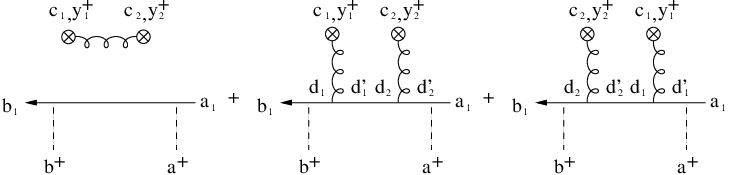
Refer to caption
Figure 5: Diagrammatic rules shown with some of the first topologies they resum. Note that for the second correlator ⟨Ua​b​(b+,a+|x⟂)​Uc​d​(b+,a+|y⟂)⟩\langle U_{ab}(b^{+},a^{+}|x_{\perp})U_{cd}(b^{+},a^{+}|y_{\perp})\rangle, only the ladder-like diagram are allowed since all other topologies have no support and are zero [58, 59]. Finally, in this notation, the light-cone coordinates are ordered following the arrow, from left (the smallest) to right (the biggest) so that b+>a+b^{+}>a^{+}.
Refer to caption
Figure 6: Diagrammatic representation of the 1 Wilson line - 2 color charge densities correlator F2,1​(b+,a+)F^{2,1}(b^{+},a^{+}). The first figure corresponds to the contraction of two external sources. The other figures represent the cases where the external sources are contracted with internal sources. The indices a1,b1,c1,c2,d1,d1′,d2,d2′a_{1},b_{1},c_{1},c_{2},d_{1},d^{\prime}_{1},d_{2},d^{\prime}_{2} are color indices while a+,b+,y1+,y2+a^{+},b^{+},y_{1}^{+},y_{2}^{+} are light-cone coordinates.
F2,1​(b+,a+)\displaystyle F^{2,1}(b^{+},a^{+}) =\displaystyle= ⟨ρc1​(y1+,y1⟂)​ρc2​(y2+,y2⟂)⟩​⟨Ua1​b1​(b+,a+|x1⟂)⟩\displaystyle\langle\rho_{c_{1}}(y_{1}^{+},y_{1\perp})\rho_{c_{2}}(y_{2}^{+},y_{2\perp})\rangle\langle U_{a_{1}b_{1}}(b^{+},a^{+}|x_{1\perp})\rangle (49)
+\displaystyle+ θ⁡(y1+−y2+)​μ2​(y1+)​μ2​(y2+)​fc1​d1​d1′​fc2​d2​d2′​G0​(y1⟂−x1⟂)​G0​(y2⟂−x1⟂)\displaystyle\theta(y_{1}^{+}-y_{2}^{+})\mu^{2}(y_{1}^{+})\mu^{2}(y_{2}^{+})f_{c_{1}d_{1}d^{\prime}_{1}}f_{c_{2}d_{2}d^{\prime}_{2}}G_{0}(y_{1\perp}-x_{1\perp})G_{0}(y_{2\perp}-x_{1\perp})
×⟨Ub1​d1​(b+,y1+|x1⟂)⟩​⟨Ud1′​d2​(y1+,y2+|x1⟂)⟩​⟨Ud2′​a1​(y2+,a+|x1⟂)⟩\displaystyle\times\langle U_{b_{1}d_{1}}(b^{+},y_{1}^{+}|x_{1\perp})\rangle\langle U_{d^{\prime}_{1}d_{2}}(y_{1}^{+},y_{2}^{+}|x_{1\perp})\rangle\langle U_{d^{\prime}_{2}a_{1}}(y_{2}^{+},a^{+}|x_{1\perp})\rangle
+\displaystyle+ θ⁡(y2+−y1+)​μ2​(y1+)​μ2​(y2+)​fc1​d1​d1′​fc2​d2​d2′​G0​(y1⟂−x1⟂)​G0​(y2⟂−x1⟂)\displaystyle\theta(y_{2}^{+}-y_{1}^{+})\mu^{2}(y_{1}^{+})\mu^{2}(y_{2}^{+})f_{c_{1}d_{1}d^{\prime}_{1}}f_{c_{2}d_{2}d^{\prime}_{2}}G_{0}(y_{1\perp}-x_{1\perp})G_{0}(y_{2\perp}-x_{1\perp}) (50)
×⟨Ub1​d2​(b+,y2+|x1⟂)⟩​⟨Ud2′​d1​(y2+,y1+|x1⟂)⟩​⟨Ud1′​a1​(y1+,a+|x1⟂)⟩.\displaystyle\times\langle U_{b_{1}d_{2}}(b^{+},y_{2}^{+}|x_{1\perp})\rangle\langle U_{d^{\prime}_{2}d_{1}}(y_{2}^{+},y_{1}^{+}|x_{1\perp})\rangle\langle U_{d^{\prime}_{1}a_{1}}(y_{1}^{+},a^{+}|x_{1\perp})\rangle.

This can be simplified further by using the explicit expressions given in Eqs. (34), (37) and (46). We get that

F2,1​(b+,a+)\displaystyle F^{2,1}(b^{+},a^{+}) =\displaystyle= δc1​c2​δa1​b1​μ2​(y1+)​δ​(y1+−y2+)​δ2​(y1⟂−y2⟂)​U¯​(b+,a+|x1⟂)\displaystyle\delta_{c_{1}c_{2}}\delta_{a_{1}b_{1}}\mu^{2}(y_{1}^{+})\delta(y_{1}^{+}-y_{2}^{+})\delta^{2}(y_{1\perp}-y_{2\perp})\bar{U}(b^{+},a^{+}|x_{1\perp}) (51)
+\displaystyle+ μ2​(y1+)​μ2​(y2+)​G0​(x1⟂−y1⟂)​G0​(x1⟂−y2⟂)​U¯​(b+,a+|x1⟂)\displaystyle\mu^{2}(y_{1}^{+})\mu^{2}(y_{2}^{+})G_{0}(x_{1\perp}-y_{1\perp})G_{0}(x_{1\perp}-y_{2\perp})\bar{U}(b^{+},a^{+}|x_{1\perp})
×(fc1​b1​d​fc2​d​a1​θ​(y1+−y2+)+fc2​b1​d​fc1​d​a1​θ​(y2+−y1+))\displaystyle\times(f_{c_{1}b_{1}d}f_{c_{2}da_{1}}\theta(y_{1}^{+}-y_{2}^{+})+f_{c_{2}b_{1}d}f_{c_{1}da_{1}}\theta(y_{2}^{+}-y_{1}^{+}))

Considering that the nuclei is moving at the speed of light and integrating on both sides by y1+y_{1}^{+} and y2+y_{2}^{+}, we get

⟨Ua​b​(b+,a+|x1⟂)​ρc1​(y1⟂)​ρc2​(y2⟂)⟩\displaystyle\langle U_{ab}(b^{+},a^{+}|x_{1\perp})\rho_{c_{1}}(y_{1\perp})\rho_{c_{2}}(y_{2\perp})\rangle =\displaystyle= δc1​c2​δa1​b1​μA2​δ2​(y1⟂−y2⟂)​U¯​(b+,a+|x1⟂)\displaystyle\delta_{c_{1}c_{2}}\delta_{a_{1}b_{1}}\mu^{2}_{A}\delta^{2}(y_{1\perp}-y_{2\perp})\bar{U}(b^{+},a^{+}|x_{1\perp}) (52)
+\displaystyle+ μc4​G0​(x1⟂−y1⟂)​G0​(x1⟂−y2⟂)​U¯​(b+,a+|x1⟂)\displaystyle\mu_{c}^{4}G_{0}(x_{1\perp}-y_{1\perp})G_{0}(x_{1\perp}-y_{2\perp})\bar{U}(b^{+},a^{+}|x_{1\perp})
×(fc1​b1​d​fc2​d​a1+fc2​b1​d​fc1​d​a1)\displaystyle\times(f_{c_{1}b_{1}d}f_{c_{2}da_{1}}+f_{c_{2}b_{1}d}f_{c_{1}da_{1}})

where we defined

μc4=∫−∞∞d​u+​∫u+∞d​v+​μ2​(u+)​μ2​(v+).\displaystyle\mu_{c}^{4}=\int_{-\infty}^{\infty}du^{+}\int_{u^{+}}^{\infty}dv^{+}\mu^{2}(u^{+})\mu^{2}(v^{+}). (53)

IV.3 2 Wilson lines - 2 color charges densities correlator

In this subsection, we compute the correlator

F2,2​(b+,a+)≡⟨Ua1​b1​(b+,a+|x1⟂)​Ua2​b2​(b+,a+|x2⟂)​ρc1​(y1+,y1⟂)​ρc2​(y2+,y2⟂)⟩.\displaystyle F^{2,2}(b^{+},a^{+})\equiv\langle U_{a_{1}b_{1}}(b^{+},a^{+}|x_{1\perp})U_{a_{2}b_{2}}(b^{+},a^{+}|x_{2\perp})\rho_{c_{1}}(y_{1}^{+},y_{1\perp})\rho_{c_{2}}(y_{2}^{+},y_{2\perp})\rangle. (54)

This calculation is similar to the one of the second correlator F2,1F^{2,1} using the diagrammatic rules. Three typical diagrams of F2,2​(b+,a+)F^{2,2}(b^{+},a^{+}) out of seven are shown in Fig. 7. The first one corresponds to the contraction of the two external sources and the other ones corresponds the connected part which consists in all contractions between internal and external sources.

The first diagram is straightforward to compute. It is given by

F12,2​(b+,a+)≡⟨Ua1​b1​(b+,a+|x1⟂)​Ua2​b2​(b+,a+|x2⟂)⟩​⟨ρc1​(y1+,y1⟂)​ρc2​(y2+,y2⟂)⟩.\displaystyle F^{2,2}_{1}(b^{+},a^{+})\equiv\langle U_{a_{1}b_{1}}(b^{+},a^{+}|x_{1\perp})U_{a_{2}b_{2}}(b^{+},a^{+}|x_{2\perp})\rangle\langle\rho_{c_{1}}(y_{1}^{+},y_{1\perp})\rho_{c_{2}}(y_{2}^{+},y_{2\perp})\rangle. (55)

Using Eqs. (34) and (38), we get that

F12,2​(b+,a+)\displaystyle F^{2,2}_{1}(b^{+},a^{+}) =\displaystyle= μ2(y1+)δ(y1+−y2+)δ2(y1⟂−y2⟂)V¯(b+,a+|x1⟂,x2⟂)δc1​c2​δa1​a2​δb1​b2Nc2−1.\displaystyle\mu^{2}(y_{1}^{+})\delta(y_{1}^{+}-y_{2}^{+})\delta^{2}(y_{1\perp}-y_{2\perp})\bar{V}(b^{+},a^{+}|x_{1\perp},x_{2\perp})\frac{\delta_{c_{1}c_{2}}\delta_{a_{1}a_{2}}\delta_{b_{1}b_{2}}}{N_{c}^{2}-1}. (56)
Refer to caption
Figure 7: These are the first few diagrams included in the calculation of F2,2​(b+,a+)F^{2,2}(b^{+},a^{+}). They differ essentially by the way the sources are inserted between the blobs.

The second diagram shown in Fig. 7 is given by

F22,2​(b+,a+)\displaystyle F^{2,2}_{2}(b^{+},a^{+}) =\displaystyle= θ⁡(y1+−y2+)​μ2​(y1+)​μ2​(y2+)​fc1​d1​d1′​fc2​d2​d2′​G0​(y1⟂−x1⟂)​G0​(y2⟂−x1⟂)\displaystyle\theta(y_{1}^{+}-y_{2}^{+})\mu^{2}(y_{1}^{+})\mu^{2}(y_{2}^{+})f_{c_{1}d_{1}d^{\prime}_{1}}f_{c_{2}d_{2}d^{\prime}_{2}}G_{0}(y_{1\perp}-x_{1\perp})G_{0}(y_{2\perp}-x_{1\perp}) (58)
×⟨Ub1​d1​(b+,y1+|x1⟂)​Ub2​β1(2)​(b+,y1+|x2⟂)⟩​⟨Ud1′​d2​(y1+,y2+|x1⟂)​Uβ1(2)​β2(2)​(y1+,y2+|x2⟂)⟩\displaystyle\times\langle U_{b_{1}d_{1}}(b^{+},y_{1}^{+}|x_{1\perp})U_{b_{2}\beta_{1}^{(2)}}(b^{+},y_{1}^{+}|x_{2\perp})\rangle\langle U_{d^{\prime}_{1}d_{2}}(y_{1}^{+},y_{2}^{+}|x_{1\perp})U_{\beta_{1}^{(2)}\beta_{2}^{(2)}}(y_{1}^{+},y_{2}^{+}|x_{2\perp})\rangle
×⟨Ud2′​a1​(y2+,a+|x1⟂)​Uβ2(2)​a2​(y2+,a+|x2⟂)⟩.\displaystyle\times\langle U_{d^{\prime}_{2}a_{1}}(y_{2}^{+},a^{+}|x_{1\perp})U_{\beta_{2}^{(2)}a_{2}}(y_{2}^{+},a^{+}|x_{2\perp})\rangle.

Using Eqs. (37) and (38), we get

F22,2​(b+,a+)\displaystyle F^{2,2}_{2}(b^{+},a^{+}) =\displaystyle= θ⁡(y1+−y2+)​μ2​(y1+)​μ2​(y2+)​fc1​d1​d1​fc2​d2​d2​G0​(y1⟂−x1⟂)​G0​(y2⟂−x1⟂)\displaystyle\theta(y_{1}^{+}-y_{2}^{+})\mu^{2}(y_{1}^{+})\mu^{2}(y_{2}^{+})f_{c_{1}d_{1}d_{1}}f_{c_{2}d_{2}d_{2}}G_{0}(y_{1\perp}-x_{1\perp})G_{0}(y_{2\perp}-x_{1\perp}) (59)
×V¯(b+,y1+|x1⟂,x2⟂)V¯(y1+,y2+|x1⟂,x2⟂)V¯(y2+,a+|x1⟂,x2⟂)\displaystyle\times\bar{V}(b^{+},y_{1}^{+}|x_{1\perp},x_{2\perp})\bar{V}(y_{1}^{+},y_{2}^{+}|x_{1\perp},x_{2\perp})\bar{V}(y_{2}^{+},a^{+}|x_{1\perp},x_{2\perp})
=\displaystyle= 0\displaystyle 0 (60)

which is zero because of the color structure. All the other diagrams included in F2,2​(b+,a+)F^{2,2}(b^{+},a^{+}) can be computed in a similar way. There are five other different ways of inserting the source and they all vanish because of the color structure. The only non-zero term is the first one and so we have F2,2​(b+,a+)=F12,2​(b+,a+)F^{2,2}(b^{+},a^{+})=F^{2,2}_{1}(b^{+},a^{+}). Finally, with a nucleus moving at the speed of light, we obtain

⟨Ua1​b1​(b+,a+|x1⟂)​Ua2​b2​(b+,a+|x2⟂)​ρc1​(y1⟂)​ρc2​(y2⟂)⟩\displaystyle\langle U_{a_{1}b_{1}}(b^{+},a^{+}|x_{1\perp})U_{a_{2}b_{2}}(b^{+},a^{+}|x_{2\perp})\rho_{c_{1}}(y_{1\perp})\rho_{c_{2}}(y_{2\perp})\rangle =\displaystyle= μA2​δ2​(y1⟂−y2⟂)​δc1​c2​δa1​a2​δb1​b2Nc2−1\displaystyle\mu_{A}^{2}\delta^{2}(y_{1\perp}-y_{2\perp})\frac{\delta_{c_{1}c_{2}}\delta_{a_{1}a_{2}}\delta_{b_{1}b_{2}}}{N_{c}^{2}-1} (61)
×V¯(b+,a+|x1⟂,x2⟂).\displaystyle\times\bar{V}(b^{+},a^{+}|x_{1\perp},x_{2\perp}).

This concludes the computation of correlators. We are now in a position to evaluate the cross section within the MV model.

V Numerical evaluation of the cross section

V.1 Proton-proton case

In this section, we evaluate the cross section numerically in p​ppp collisions. This is done by using the expression of the cross section given by Eq. (33) which can be obtained either from the dilute limit of the p​ApA result or from k⟂k_{\perp}-factorization techniques (see Appendix A). In p​ppp collisions, the cross section is related to uPDF that describe the distribution of gluons inside each protons. There exist many parametrizations of these distribution functions differing mainly in the way the evolution equation is solved. Among the most successful ones are (the description of these parametrizations can be found in [9] 11 1 We would like to thanks H. Jung for handing us his FORTRAN routine CAUNIGLU which evaluates numerically all of these parametrizations. It can be found at http://www.desy.de/ jung/cascade/updf.html. ):

  • •

    DIG (Derivative of the Integrated Gluon distribution function)

  • •

    CCFM (Catani, Ciafaloni, Fiorani, Marchesini) [60, 61, 62, 63, 8, 64]

  • •

    KMR (Kimber, Martin, Ryskin) [65]

These parametrizations are used to compute the cross section for η′\eta^{\prime} production in p​ppp collisions and to compare with the result for p​ApA collisions at small saturation scale.

The final result is obtained by integrating Eq. (33) using the VEGAS and the CUHRE algorithms implemented in the CUBA package [66]. The number of color is set to Nc=3N_{c}=3, the center of mass energy to s≈200​GeV\sqrt{s}\approx 200\;\mbox{GeV} (RHIC) and the mass of η′\eta^{\prime} to M=0.957​GeVM=0.957\;\mbox{GeV}. To make a comparison with p​ApA collisions for a wide range of transverse momentum where the MV model is valid (see Fig. (9)), we chose the rapidity y=1y=1. The results of the numerical calculation are shown in Fig. (8) where we also present the result for the p​ApA case at small saturation scale (Qs2=1​GeVQ_{s}^{2}=1\;\mbox{GeV}) and with the proton described by the parametrization CCFM J2003 set 3.

Refer to caption
Figure 8: Numerical results of the inclusive differential cross section at rapidity (y=1y=1) and at RHIC energy (s\sqrt{s}=200 GeV). The results for p​ppp collisions are scaled by the number of nucleons AA to make a comparison with p​ApA. The cross section for p​ApA collisions is evaluated at the saturation scale Qs=1​GeVQ_{s}=1\;\mbox{GeV}.

V.2 Proton-nucleus case using the MV model

We now consider η′\eta^{\prime} production for p​ApA collisions for which the cross section is given by Eq. (31). This formal expression can be simplified by using the results of section IV where the correlators of Wilson lines are evaluated in the MV model. Note here that in the MV model, the nucleus is considered as an infinite source of charge in the transverse plane so there are no edge effects. In this kind of description, translation invariance in the transverse plane is preserved and therefore the correlators have the following property

⟨ρA,a​(x⟂)​ρA,b​(y⟂)​Uc​e​(z⟂)​Uc′​e′​(w⟂)⟩=⟨ρA,a​(x⟂−w⟂)​ρA,b​(y⟂−w⟂)​Uc​e​(z⟂−w⟂)​Uc′​e′​(0)⟩.\displaystyle\langle\rho_{A,a}(x_{\perp})\rho_{A,b}(y_{\perp})U_{ce}(z_{\perp})U_{c^{\prime}e^{\prime}}(w_{\perp})\rangle=\langle\rho_{A,a}(x_{\perp}-w_{\perp})\rho_{A,b}(y_{\perp}-w_{\perp})U_{ce}(z_{\perp}-w_{\perp})U_{c^{\prime}e^{\prime}}(0)\rangle. (62)

Then, we can write

(2​π)3​2​Ek​d​σd3​k\displaystyle(2\pi)^{3}2E_{k}\frac{d\sigma}{d^{3}k} ≈\displaystyle\approx g2​π2(Nc2−1)​∫d2​p⟂​d2​q⟂​d2​r⟂(2​π)6​F​(−p⟂2,−p2,⟂2)​F∗​(−q⟂2,−q2,⟂2)\displaystyle\frac{g^{2}\pi^{2}}{(N_{c}^{2}-1)}\int\frac{d^{2}p_{\perp}d^{2}q_{\perp}d^{2}r_{\perp}}{(2\pi)^{6}}F(-p_{\perp}^{2},-p_{2,\perp}^{2})F^{*}(-q_{\perp}^{2},-q_{2,\perp}^{2}) (63)
×[⟨ρA,a∗(p⟂)ρA,a(q⟂)⟩(2π)2δ2(p2,⟂−r⟂)(2π)2δ2(q2,⟂−r⟂)\displaystyle\times\biggl[\langle\rho_{A,a}^{*}(p_{\perp})\rho_{A,a}(q_{\perp})\rangle(2\pi)^{2}\delta^{2}(p_{2,\perp}-r_{\perp})(2\pi)^{2}\delta^{2}(q_{2,\perp}-r_{\perp})
+∫d2x⟂d2y⟂d2z⟂d2w⟂ei​p⟂⋅x⟂−i​q⟂⋅y⟂+i⁡(p2,⟂−r⟂)⋅z⟂−i⁡(q2,⟂−r⟂)⋅w⟂\displaystyle+\int d^{2}x_{\perp}d^{2}y_{\perp}d^{2}z_{\perp}d^{2}w_{\perp}e^{ip_{\perp}\cdot x_{\perp}-iq_{\perp}\cdot y_{\perp}+i(p_{2,\perp}-r_{\perp})\cdot z_{\perp}-i(q_{2,\perp}-r_{\perp})\cdot w_{\perp}}
×⟨ρA,a(x⟂)ρA,b(y⟂)Ua​c(z⟂)Ub​c(w⟂)⟩]ϵi​jϵk​lpi​qk​rj​rlp⟂2​q⟂2​r⟂2ϕp(r⟂2,x).\displaystyle\times\langle\rho_{A,a}(x_{\perp})\rho_{A,b}(y_{\perp})U_{ac}(z_{\perp})U_{bc}(w_{\perp})\rangle\biggr]\epsilon_{ij}\epsilon_{kl}\frac{p^{i}q^{k}r^{j}r^{l}}{p^{2}_{\perp}q^{2}_{\perp}r_{\perp}^{2}}\phi_{p}(r_{\perp}^{2},x).

To obtain this expression, we used Eq. (9) to convert the average on proton sources to an unintegrated distribution function and we Fourier transformed the correlator in the second term. We also neglected all terms with only one Wilson line because they are numerically very small compared to the other terms. This can be seen as follows. First, using translation invariance of the correlator, we see that averages with one Wilson line in the cross section are proportional to U¯​(0)\bar{U}(0) (see Eq. (62)). This quantity is small because there is an infrared singularity appearing in the argument of the exponential in the following way [59]:

U¯​(0)\displaystyle\bar{U}(0) =\displaystyle= exp[−Nc2L(0,0)Qs]=exp[−Nc2Qs2∫d2​p⟂(2​π)21p⟂4]≈0.\displaystyle\exp\left[-\frac{N_{c}}{2}L(0,0)Q_{s}\right]=\exp\left[-\frac{N_{c}}{2}Q_{s}^{2}\int\frac{d^{2}p_{\perp}}{(2\pi)^{2}}\frac{1}{p_{\perp}^{4}}\right]\approx 0. (64)

This is not exactly zero because the infrared singularity is regulated by non-perturbative effects (confinement) and these induce a cutoff of order ΛQCD\Lambda_{\rm{QCD}}. The saturation scale in a large nuclei at small-xx satisfies Qs2≫ΛQCD2Q_{s}^{2}\gg\Lambda_{\rm{QCD}}^{2} so that U¯​(0)∼exp⁡[−Qs2ΛQCD2]≪1\bar{U}(0)\sim\exp\left[-\frac{Q_{s}^{2}}{\Lambda_{\rm{QCD}}^{2}}\right]\ll 1. Thus, the correlators with one Wilson line can be neglected.

It is then a straightforward calculation, involving some change of variables, translation invariance and Eqs. (34) and (61), to obtain

(2​π)3​2​Ek​d​σd3​k\displaystyle(2\pi)^{3}2E_{k}\frac{d\sigma}{d^{3}k} =\displaystyle= π2​g2​μA2​S⟂​∫d2​p⟂​d2​r⟂(2​π)4​|F⁡(−p⟂2,−p2,⟂2)|2​ϵi​j​ϵk​l​pi​pk​rj​rlp⟂2​(p⟂2+Λ2)​r⟂2\displaystyle\pi^{2}g^{2}\mu^{2}_{A}S_{\perp}\int\frac{d^{2}p_{\perp}d^{2}r_{\perp}}{(2\pi)^{4}}|F(-p_{\perp}^{2},-p_{2,\perp}^{2})|^{2}\epsilon_{ij}\epsilon_{kl}\frac{p^{i}p^{k}r^{j}r^{l}}{p^{2}_{\perp}(p^{2}_{\perp}+\Lambda^{2})r_{\perp}^{2}} (65)
×ϕp​(r⟂2,x)​[(2​π)2​δ2​(p2,⟂−r⟂)+∫d2​z⟂​ei⁡(p2,⟂−r⟂)⋅z⟂​V¯​(z⟂,0)]\displaystyle\times\phi_{p}(r_{\perp}^{2},x)\biggl[(2\pi)^{2}\delta^{2}(p_{2,\perp}-r_{\perp})+\int d^{2}z_{\perp}e^{i(p_{2,\perp}-r_{\perp})\cdot z_{\perp}}\bar{V}(z_{\perp},0)\biggr]

where S⟂=(2​π)2​δ2​(0)S_{\perp}=(2\pi)^{2}\delta^{2}(0) is interpreted as the transverse area of the nuclei. We also introduced here an infrared regulator given by Λ\Lambda in one of the denominator 1p⟂2\frac{1}{p_{\perp}^{2}}. This is because gluons separated by a distance greater than the size of a nucleon (∼1​fm\sim 1\;\mbox{fm}) are not correlated because of confinement so that Λ=ΛQCD\Lambda=\Lambda_{\rm{QCD}}. This is not taken into account explicitly in the MV model, leading to infrared divergent quantities [67] which are regulated by adding the infrared regulator [56]. This is equivalent to define a gluon distribution function for the MV model as

ϕA​(x,p⟂,Q2)=αs​(Nc2−1)​A2​π​1p⟂2+Λ2.\displaystyle\phi_{A}(x,p_{\perp},Q^{2})=\frac{\alpha_{s}(N_{c}^{2}-1)A}{2\pi}\frac{1}{p_{\perp}^{2}+\Lambda^{2}}. (66)

We do not introduce a regulator in the other denominator 1p⟂2\frac{1}{p_{\perp}^{2}} because as seen in Eq. (77), it is part of the matrix element |ℳ|2∼ϵi​j​ϵk​l​pi​pk​rj​rlp⟂2​r⟂2|\mathcal{M}|^{2}\sim\epsilon_{ij}\epsilon_{kl}\frac{p^{i}p^{k}r^{j}r^{l}}{p^{2}_{\perp}r_{\perp}^{2}} which is well behaved in the infrared.

In the first term of the cross section, one integration can be done easily with the delta function. The remaining integrals will be done numerically. The second term can be simplified further by doing some integrals analytically as shown in Appendix B. The first term is very similar to the p​ppp cross section and does not involve any saturation scale dependence because it does not include any multiscatterings. The QsQ_{s} dependence occurs in the second term through the expression of V¯\bar{V} where we define it as

Qs2=Nc​μA2​g42​π.\displaystyle Q_{s}^{2}=\frac{N_{c}\mu_{A}^{2}g^{4}}{2\pi}. (67)

V.2.1 Kinematical range

The cross section derived in the previous section is restricted to a certain range of validity because we are using the MV model. This model can be used when the radiative corrections which goes like αs​ln⁡(1/x)\alpha_{s}\ln(1/x) are not too large, which is when 0.01≲xA≲0.10.01\lesssim x_{A}\lesssim 0.1. For η′\eta^{\prime} production, the momentum fraction of gluons in the proton and the nucleus are given by

xp\displaystyle x_{p} =\displaystyle= M2+k⟂2s​ey,\displaystyle\sqrt{\frac{M^{2}+k_{\perp}^{2}}{s}}e^{y}, (68)
xA\displaystyle x_{A} =\displaystyle= M2+k⟂2s​e−y.\displaystyle\sqrt{\frac{M^{2}+k_{\perp}^{2}}{s}}e^{-y}. (69)

The kinematic range in terms of the η′\eta^{\prime} transverse momentum and rapidity where 0.01≲xA≲0.10.01\lesssim x_{A}\lesssim 0.1 is depicted in Fig. 9 for RHIC energies.

It is possible to extend the range of validity to smaller values of xAx_{A} by using the JIMWLK equation [41, 42, 43, 44, 45]. This renormalization group equation resums the large radiative corrections due to very small xx modes. The effect is to change the correlation between sources and in general, one looses the Gaussian structure of the weight functional W⁡[ρ]W[\rho]. This complicates the computation of Wilson line correlators and is outside the scope of this article.

Refer to caption
Figure 9: The grey region is the kinematic range where the calculation using the MV model is valid for RHIC energies in terms of the η′\eta^{\prime} transverse momentum k=|k⟂|k=|k_{\perp}| and rapidity yy.

V.2.2 Numerical Results

We present in this section the numerical results for η′\eta^{\prime} production. We integrate numerically Eq. (84) and the first term of Eq. (65) using the same values for the parameters as in p​ppp collisions. The strong coupling constant appearing in the cross section is evaluated at the η′\eta^{\prime} transverse mass scale M⟂2M_{\perp}^{2}. The unintegrated distribution functions chosen for the protons is the CCFM J2003 set 3 because it is very successful in the description of other observables like charm and bottom production at the Tevatron [64]. The results of the numerical integration are shown in Figs. (10) and (11) for different values for the rapidity.

In Fig. (12), we show the result for the inverse nuclear modification factor Rp​AR_{pA} for y=1y=1 defined as

1Rp​A=A​d​σp​pd2​k⟂​d​yd​σp​Ad2​k⟂​d​y.\displaystyle\frac{1}{R_{pA}}=\frac{A\frac{d\sigma^{pp}}{d^{2}k_{\perp}dy}}{\frac{d\sigma^{pA}}{d^{2}k_{\perp}dy}}. (70)

We use this because the p​ppp cross section is zero at |k⟂|=0|k_{\perp}|=0.

Refer to caption
Figure 10: Numerical results of the inclusive differential cross section at midrapidity (y=0y=0) and at RHIC energy (s\sqrt{s}=200 GeV). The first curve is the result of the cross section for p​ppp collisions scaled by the number of nucleons AA. The other curves are the results for the cross section for p​ApA collisions for different values of the saturation scale (QsQ_{s}=1,4 and 10 GeV).
Refer to caption
Figure 11: Numerical results of the inclusive differential cross section at rapidity y=1y=1 and at RHIC energy (s\sqrt{s}=200 GeV). The first curve is the result of the cross section for p​ppp collisions scaled by the number of nucleons AA. The other curves are the results for the cross section for p​ApA collisions for different values of the saturation scale (QsQ_{s}=1,4 and 10 GeV).
Refer to caption
Figure 12: Numerical results for the inverse nuclear modification factor at rapidity (y=1y=1) and at RHIC energy (s\sqrt{s}=200 GeV). We show the results for different values of the saturation scale (QsQ_{s}=1,4 and 10 GeV).

V.3 Analysis

For the p​ppp cross section, there is a wide range of variability for the cross section depending on the parametrization of the uPDF used. This feature can be used to discriminate between the different parametrizations to determine the most accurate one. Thus, by combining this analysis with experimental data, the η′\eta^{\prime} production becomes another observable that can be utilized to constrain models of uPDF. A similar conclusion was reached in [31] where the f2f_{2}-meson production was studied. Note however that the results of the cross section at small transverse momentum should be treated carefully. As stated in the appendix A, the validity of the k⟂k_{\perp}-factorization approach depends on the presence of a large scale compared to the QCD scale given in our case by Q2∼M⟂2Q^{2}\sim M_{\perp}^{2}. At very small momentum, we have that M⟂2ΛQCD2≈23\frac{M_{\perp}^{2}}{\Lambda_{\rm{QCD}}^{2}}\approx 23 for which the semihard inequality ΛQCD2≪Q2≪s\Lambda_{\rm{QCD}}^{2}\ll Q^{2}\ll\sqrt{s} that guarantees the accuracy of k⟂k_{\perp}-factorization is only marginally satisfied. Thus, at small momentum, the cross section should be seen as an extrapolation of the k⟂k_{\perp}-factorized cross section to a regime where k⟂k_{\perp}-factorization cannot be rigorously proven.

The p​ApA cross section shows a strong dependence on the saturation scale. As QsQ_{s} becomes smaller, the magnitude of the cross section looks more like the p​ppp cross section. On the other hand, the cross section diminishes as QsQ_{s} becomes larger. This can be understood in the following way. The saturation scale is defined as the momentum at which the probability of interaction between different parton cascades is of order one [14, 15]. The partons having a transverse size satisfying δ​x⟂∼1Q⟂≥1Qs\delta x_{\perp}\sim\frac{1}{Q_{\perp}}\geq\frac{1}{Q_{s}} will have a very high probability to recombine. As the saturation scale is increased, there will be more gluons that will be sensitive to these nonlinear effects. The final result is that as more and more gluons have a high probability to recombine, the growth of their population will decrease and so is the cross section for a given set of parameters. This effect is clearly seen in the cross section computed in our model. The fact that the η′\eta^{\prime} production cross section is sensitive to the saturation scale can be used to estimate the numerical value of QsQ_{s}. The current estimate based on HERA data for deep inelastic scattering shows that for RHIC energy, it is given by Qs∼1−2​GeVQ_{s}\sim 1-2\;\mbox{GeV} [14, 15]. It would be interesting to compare our calculation to experimental data to make an estimation of QsQ_{s} based on η′\eta^{\prime} production and see if it is consistent with the previous estimation.

The nuclear modification factor shows clearly the saturation effects for 0.4≲|k⟂|≲3.40.4\lesssim|k_{\perp}|\lesssim 3.4 because in that range, Rp​A>1R_{pA}>1. At large transverse momentum, it approaches the value Rp​A≈0.45R_{pA}\approx 0.45. One would expect Rp​AR_{pA} to be one in that range of momentum because it corresponds to the regime where there are no saturation effects and where the k⟂k_{\perp}-factorized cross section can be used. This discrepancy can be explained by looking at the approximations made during the calculation. We neglect two terms in the cross section that are proportional to one Wilson line (see Eq. (64)). In the dilute limit (when |k⟂|>Qs|k_{\perp}|>Q_{s}), these terms cannot be neglected and have a non zero contribution that would make Rp​A≈1R_{pA}\approx 1. In that sense, our approximation fails at large transverse momentum and our result should be treated carefully in that regime.

VI Conclusion

In this article, the inclusive cross section for η′\eta^{\prime} production in p​ppp and p​ApA collisions is computed. The p​ppp case is analyzed for different reasons. First, it serves as a basis to validate our model for η′\eta^{\prime} production against experimental data. This model includes two main ingredients. The first one is the effective theory which is at the foundation of our analysis. We use in our study a very simplified form of this effective theory where the vertex is given by Eq. (3). As shown in [19, 20, 21, 22, 23, 24, 25], this is a very crude approximation of the real vertex, so there are some improvements that can be done in this direction in the future. The second ingredient are the uPDF parametrizations. As seen in Fig. (8), there is still a large variability in the predictions made by different uPDF. Therefore, η′\eta^{\prime} production could be used to constrain the models of uPDF once it is compared to experimental data. The same conclusion was obtained in [26] for the exclusive process p+p→p+p+η′p+p\rightarrow p+p+\eta^{\prime}. Finally, from the theoretical point of view, we studied p​ppp collisions to see if the cross section can be obtained as the low density limit of the p​ApA cross section. There are now many known examples where this can be seen like gluon production [56, 68, 50], quark production [57, 48] and tensor meson production [31]. We have shown that η′\eta^{\prime} production also obeys this property and in that sense, it is a consistency check for the approach used for the p​ApA case.

The p​ApA results for the η′\eta^{\prime} inclusive cross section show some very interesting features. First, we show that they are sensitive to the value of the saturation scale. This can also be seen in the plot of the nuclear modification factor. This property could be used to make an estimate of QsQ_{s} by comparing with experimental data, which is one of the main goal of our analysis. This information is very important for the study of other particle production such as quark and gluon production in both p​ApA and A​AAA where saturation effects play an important role. Thus, a measurement of η′\eta^{\prime} at RHIC would improve our knowledge of gluon distribution in a nucleus.

Throughout the article, we assumed that the gluon fusion process was the dominant mechanism in η′\eta^{\prime} production. There is one other production process that could also be important. It is the photon fusion where two off-shell photons emitted by the protons or the nucleus merge to give a η′\eta^{\prime} such as γ∗+γ∗→η′+X\gamma^{*}+\gamma^{*}\rightarrow\eta^{\prime}+X. This is estimated in [26] and according to this analysis, it should be subdominant in the exclusive production. We assume that this holds also in our study, although a careful analysis of this process should be performed. Of course, our calculation could be made more accurate by investigating this last issue.

Acknowledgements.
The authors want to thank F. Gelis, R. Venugopalan, T. Lappi, Y. Kovchegov, K. Tuchin and J.-S. Gagnon for interesting and stimulating discussions.

Appendix A Cross section in p​ppp collisions

The calculation of the cross section for η′\eta^{\prime} production in proton-proton collisions at RHIC can be performed in the k⟂k_{\perp}-factorization formalism. This formalism can be used in the semihard regime where the factorization scale satisfies the inequality ΛQCD2≪Q2≪s\Lambda_{\rm{QCD}}^{2}\ll Q^{2}\ll\sqrt{s}. For η′\eta^{\prime}, this inequality is only marginally satisfied at small transverse momentum because its mass is relatively low. It is recovered at larger transverse momentum, around |k⟂|∼2−3​GeV|k_{\perp}|\sim 2-3\;\mbox{GeV}. The starting point is the usual formula of the inclusive cross section in k⟂k_{\perp}-factorization:

(2​π)3​2​Ek​d​σp​p→η′​Xd3​k\displaystyle(2\pi)^{3}2E_{k}\frac{d\sigma^{pp\rightarrow\eta^{\prime}X}}{d^{3}k} =\displaystyle= 16​π2​∫01d​x1x1​d​x2x2​∫d2​q⟂​d2​p⟂(2​π)4​ϕ1​(x1,p⟂2,Q2)​ϕ2​(x2,q⟂2,Q2)\displaystyle 16\pi^{2}\int_{0}^{1}\frac{dx_{1}}{x_{1}}\frac{dx_{2}}{x_{2}}\int\frac{d^{2}q_{\perp}d^{2}p_{\perp}}{(2\pi)^{4}}\phi_{1}(x_{1},p_{\perp}^{2},Q^{2})\phi_{2}(x_{2},q_{\perp}^{2},Q^{2}) (71)
×(2​π)3​2​Ek​d​σg∗​g∗→η′​Xd3​k\displaystyle\times(2\pi)^{3}2E_{k}\frac{d\sigma^{g^{*}g^{*}\rightarrow\eta^{\prime}X}}{d^{3}k}

where

(2​π)3​2​Ek​d​σg∗​g∗→Hd3​k=12​s^​|ℳg∗​g∗→η′|2​(2​π)4​δ4​(p+q−k)\displaystyle(2\pi)^{3}2E_{k}\frac{d\sigma^{g^{*}g^{*}\rightarrow H}}{d^{3}k}=\frac{1}{2\hat{s}}|\mathcal{M}^{g^{*}g^{*}\rightarrow\eta^{\prime}}|^{2}(2\pi)^{4}\delta^{4}(p+q-k) (72)

is the high-energy limit of the cross section for off-shell gluons g∗g^{*} to on-shell η′\eta^{\prime} mesons, s^=x1​x2​s\hat{s}=x_{1}x_{2}s is the k⟂k_{\perp}-factorization flux factor [1, 2], x1,2x_{1,2} are momentum fractions of gluons and ϕ1,2​(x1,2,k⟂,Q2)\phi_{1,2}(x_{1,2},k_{\perp},Q^{2}) are unintegrated gluon distribution functions of proton 1 and 2. The unintegrated distribution functions are related to usual parton distribution functions of gluons (appearing in collinear factorization ) by

∫0Q2d​k⟂2​ϕ​(x,k⟂2,Q2)≈x​G​(x,Q2)\displaystyle\int_{0}^{Q^{2}}dk_{\perp}^{2}\phi(x,k_{\perp}^{2},Q^{2})\approx xG(x,Q^{2}) (73)

where G⁡(x,Q2)G(x,Q^{2}) is the usual gluon distribution function in collinear factorization.

To compute the production cross section of η′\eta^{\prime} mesons, the high energy limit of the lowest order matrix element between two off-shell gluons and one on-shell η′\eta^{\prime} has to be calculated. This can be evaluated by using Feynman rules where the vertex, evaluated from the interaction Lagrangian, is given by Eq. (2). Note also that in k⟂k_{\perp}-factorization, the sum on polarization tensors is given by [1, 2]

∑λϵλ∗μ​(p)​ϵλν​(p)=p⟂μ​p⟂νp⟂2\displaystyle\sum_{\lambda}\epsilon^{*\mu}_{\lambda}(p)\epsilon^{\nu}_{\lambda}(p)=\frac{p^{\mu}_{\perp}p^{\nu}_{\perp}}{p_{\perp}^{2}} (74)

where p⟂μ≡(0,p⟂,0)p_{\perp}^{\mu}\equiv(0,p_{\perp},0). The sum on polarizations differs from the usual result because we are considering off-shell gluons with a virtuality given by p2=−p⟂2p^{2}=-p_{\perp}^{2}. The exact form is due to the coupling of gluons to partons through eikonal vertices as well as gauge invariance and Ward identities [2].

In the center of mass frame, the 4-momenta of partons inside the proton moving in the ±z\pm z direction in Minkowski coordinates can be written,as:

P\displaystyle P =\displaystyle= (s2,0,0,s2);Q=(s2,0,0,−s2)\displaystyle\left(\frac{\sqrt{s}}{2},0,0,\frac{\sqrt{s}}{2}\right)\;;\;Q=\left(\frac{\sqrt{s}}{2},0,0,-\frac{\sqrt{s}}{2}\right) (75)

Then, the momenta of gluons in the large energy limit (|p⟂|,|q⟂|≪s|p_{\perp}|,|q_{\perp}|\ll\sqrt{s}) are simply

p\displaystyle p =\displaystyle= (x1​s2,p⟂,x1​s2);q=(x2​s2,q⟂,−x2​s2)\displaystyle\left(\frac{x_{1}\sqrt{s}}{2},p_{\perp},\frac{x_{1}\sqrt{s}}{2}\right)\;;\;q=\left(\frac{x_{2}\sqrt{s}}{2},q_{\perp},-\frac{x_{2}\sqrt{s}}{2}\right) (76)

Using this kinematics, it is possible to compute the high-energy limit of the matrix element ℳ\mathcal{M}. This can then be inserted in the expression of the cross section which is finally given by (see [13, 12, 31] for more details and similar calculations)

(2​π)3​2​Ek​d​σp​p→η′​Xd3​k\displaystyle(2\pi)^{3}2E_{k}\frac{d\sigma^{pp\rightarrow\eta^{\prime}X}}{d^{3}k} =\displaystyle= 4​π2(Nc2−1)​∫d2​p⟂​d2​q⟂​ϕ1​(x+,p⟂2,Q2)​ϕ2​(x−,q⟂2,Q2)\displaystyle\frac{4\pi^{2}}{(N_{c}^{2}-1)}\int d^{2}p_{\perp}d^{2}q_{\perp}\phi_{1}(x_{+},p_{\perp}^{2},Q^{2})\phi_{2}(x_{-},q_{\perp}^{2},Q^{2}) (77)
×δ2​(k⟂−p⟂−q⟂)​|F⁡(−p⟂2,−q⟂2)|2​[ϵi​j​pi​qj]2p⟂2​q⟂2\displaystyle\times\delta^{2}(k_{\perp}-p_{\perp}-q_{\perp})|F(-p_{\perp}^{2},-q_{\perp}^{2})|^{2}\frac{\left[\epsilon_{ij}p^{i}q^{j}\right]^{2}}{p_{\perp}^{2}q_{\perp}^{2}}

where x±=M⟂s​e±yx_{\pm}=\frac{M_{\perp}}{\sqrt{s}}e^{\pm y}. This expression can be used to study the phenomenology of η′\eta^{\prime} production in p​ppp collisions.

A.1 Limit of Collinear Factorization

The procedure to recover collinear factorization cross sections from k⟂k_{\perp}-factorization is well-known [1, 6, 7, 48] and will serve as a consistency check for Eq. (77). The limit |p⟂|,|q⟂|→0|p_{\perp}|,|q_{\perp}|\rightarrow 0 has to be taken in the matrix elements and the integration on the azimuthal angle has to be performed. The last step is to use the relation Eq. (73) to make the last integral and relate the unintegrated distributions to the collinear distributions. We obtain

(2​π)3​2​Ek​d​σcoll.p​p→η′​Xd3​k\displaystyle(2\pi)^{3}2E_{k}\frac{d\sigma_{\rm{coll.}}^{pp\rightarrow\eta^{\prime}X}}{d^{3}k} =\displaystyle= π2​M2​|F⁡(0,0)|22​s​(Nc2−1)​G1​(x+′,Q2)​G2​(x−′,Q2)​(2​π)2​δ2​(k⟂)\displaystyle\frac{\pi^{2}M^{2}|F(0,0)|^{2}}{2s(N_{c}^{2}-1)}G_{1}(x^{\prime}_{+},Q^{2})G_{2}(x^{\prime}_{-},Q^{2})(2\pi)^{2}\delta^{2}(k_{\perp}) (78)

where x±′=Ms​e±yx^{\prime}_{\pm}=\frac{M}{\sqrt{s}}e^{\pm y}. This expression corresponds exactly to the well-known result for leading-order η′\eta^{\prime} production in pQCD collinear formalism [27].

Appendix B Simplification of Eq. (65)

In this Appendix, we simplify the second term of the cross section and put it in a form that can be evaluated numerically. First, using the definition of V¯\bar{V} given by Eq. (38), we can perform the integrals in the exponent and we get

V¯​(z⟂,0)\displaystyle\bar{V}(z_{\perp},0) =\displaystyle= exp{−Qs2[z⟂24(1−γ+ln[2ΛQCD​|z⟂|])\displaystyle\exp\biggl\{-Q_{s}^{2}\biggl[\frac{z_{\perp}^{2}}{4}\left(1-\gamma+\ln\left[\frac{2}{\Lambda_{\rm{QCD}}|z_{\perp}|}\right]\right) (79)
+z⟂4​ΛQCD21282F3(1,1;2,3,3|−z⟂2​ΛQCD24)]}\displaystyle+\frac{z_{\perp}^{4}\Lambda_{\rm{QCD}}^{2}}{128}\;_{2}F_{3}\left(1,1;2,3,3\left|-\frac{z_{\perp}^{2}\Lambda^{2}_{\rm{QCD}}}{4}\right.\right)\biggr]\biggr\}

where γ\gamma is Euler constant and where F32(1,1;2,3,3|z)\;{}_{2}F_{3}\left(1,1;2,3,3\left|z\right.\right) is the generalized hypergeometric series. The constant ΛQCD\Lambda_{\rm{QCD}} appears in this expression as an infrared regulator.

Then, we consider the second term of Eq. (65) given by

(2​π)3​2​Ek​d​σ2d3​k\displaystyle(2\pi)^{3}2E_{k}\frac{d\sigma_{2}}{d^{3}k} =\displaystyle= π2​g2​μA2​S⟂​∫d2​z⟂​d2​p⟂​d2​r⟂(2​π)4​|F⁡(−p⟂2,−p2,⟂2)|2​ϵi​j​ϵk​l​pi​pk​rj​rlp⟂2​(p⟂2+Λ2)​r⟂2\displaystyle\pi^{2}g^{2}\mu^{2}_{A}S_{\perp}\int d^{2}z_{\perp}\frac{d^{2}p_{\perp}d^{2}r_{\perp}}{(2\pi)^{4}}|F(-p_{\perp}^{2},-p_{2,\perp}^{2})|^{2}\epsilon_{ij}\epsilon_{kl}\frac{p^{i}p^{k}r^{j}r^{l}}{p^{2}_{\perp}(p^{2}_{\perp}+\Lambda^{2})r_{\perp}^{2}} (80)
×ϕp​(r⟂2,x)​ei⁡(p2,⟂−r⟂)⋅z⟂​V¯​(z⟂,0).\displaystyle\times\phi_{p}(r_{\perp}^{2},x)e^{i(p_{2,\perp}-r_{\perp})\cdot z_{\perp}}\bar{V}(z_{\perp},0).

By letting v⟂=k⟂−p⟂−r⟂v_{\perp}=k_{\perp}-p_{\perp}-r_{\perp} and by using the identity

∫02​πd​θ​ei​x​cos⁡(θ)\displaystyle\int_{0}^{2\pi}d\theta e^{ix\cos(\theta)} =\displaystyle= 2​π​J0​(x)\displaystyle 2\pi J_{0}(x) (81)

(where J0​(x)J_{0}(x) is a Bessel function of the first kind), we find that

(2​π)3​2​Ek​d​σ2d3​k\displaystyle(2\pi)^{3}2E_{k}\frac{d\sigma_{2}}{d^{3}k} =\displaystyle= 2​π3​g2​μA2​S⟂​∫d2​p⟂​d2​v⟂(2​π)4​|F⁡(−p⟂2,−p2,⟂2)|2​ϵi​j​ϵk​l​pi​pk​(k−p−v)j​(k−p−v)lp⟂2​(p⟂2+Λ2)​(k−p−v)⟂2\displaystyle 2\pi^{3}g^{2}\mu^{2}_{A}S_{\perp}\int\frac{d^{2}p_{\perp}d^{2}v_{\perp}}{(2\pi)^{4}}|F(-p_{\perp}^{2},-p_{2,\perp}^{2})|^{2}\epsilon_{ij}\epsilon_{kl}\frac{p^{i}p^{k}(k-p-v)^{j}(k-p-v)^{l}}{p^{2}_{\perp}(p^{2}_{\perp}+\Lambda^{2})(k-p-v)_{\perp}^{2}} (82)
×ϕp​[(k−p−v)⟂2,x]​Γ​(|v⟂|).\displaystyle\times\phi_{p}[(k-p-v)_{\perp}^{2},x]\Gamma(|v_{\perp}|).

where

Γ⁡(|v⟂|)≡∫0∞d​z​z​J0​(|v⟂|​z)​V¯​(z).\displaystyle\Gamma(|v_{\perp}|)\equiv\int_{0}^{\infty}dzzJ_{0}(|v_{\perp}|z)\bar{V}(z). (83)

We let q⟂=p⟂+v⟂q_{\perp}=p_{\perp}+v_{\perp} and we use polar coordinates to get

(2​π)3​2​Ek​d​σ2d3​k\displaystyle(2\pi)^{3}2E_{k}\frac{d\sigma_{2}}{d^{3}k} =\displaystyle= αs​(M⟂2)​μA2​S⟂2​∫0∞d​p​𝑑q​∫02​πd​θ​𝑑Θ​|F⁡(−p2,−p2−k2+2​p​k​cos⁡(θ))|2\displaystyle\frac{\alpha_{s}(M_{\perp}^{2})\mu^{2}_{A}S_{\perp}}{2}\int_{0}^{\infty}dpdq\int_{0}^{2\pi}d\theta d\Theta|F(-p^{2},-p^{2}-k^{2}+2pk\cos(\theta))|^{2} (84)
×p​q​[q​sin⁡(θ−Θ)−k​sin⁡(θ)]2(p2+Λ2)​[q2+k2−2​q​k​cos⁡(Θ)]\displaystyle\times pq\frac{[q\sin(\theta-\Theta)-k\sin(\theta)]^{2}}{(p^{2}+\Lambda^{2})[q^{2}+k^{2}-2qk\cos(\Theta)]}
×ϕp​[q2+k2−2​q​k​cos⁡(Θ),x]​Γ​(|q2+p2−2​p​q​cos⁡(θ−Θ)|).\displaystyle\times\phi_{p}[q^{2}+k^{2}-2qk\cos(\Theta),x]\Gamma(|q^{2}+p^{2}-2pq\cos(\theta-\Theta)|).

where αs\alpha_{s} is the strong coupling constant. This expression is integrated numerically and the result is shown in section V.2.2.

Appendix C Computation of Eq. (31) in covariant gauge

In this Appendix, we compute the cross section by using the solution of the Yang-Mills equation in covariant gauge. This serves as a check for Eq. (31) and it shows that our result is gauge independent. The solution of the gauge field is given by Aaμ​(k)=Ap,aμ​(k)+AA,aμ​(k)+Ap​A,aμA^{\mu}_{a}(k)=A^{\mu}_{p,a}(k)+A^{\mu}_{A,a}(k)+A^{\mu}_{pA,a} where Ap,aμ​(k)A^{\mu}_{p,a}(k) is the field associated with the proton (of O⁡(ρp)O(\rho_{p})), AA,aμ​(k)A^{\mu}_{A,a}(k) is the field associated with the nuclei (of O⁡(ρA)∼O⁡(1)O(\rho_{A})\sim O(1)) and Ap​A,aμ​(k)A^{\mu}_{pA,a}(k) is the field produced by the collision (of O⁡(ρp​ρA∞)∼O⁡(ρp)O(\rho_{p}\rho_{A}^{\infty})\sim O(\rho_{p})) [50, 53]. The fields ApμA^{\mu}_{p} and Ap​AμA^{\mu}_{pA} are weak and are used as small parameters to solve the Yang-Mills equation perturbatively. The field AAμA^{\mu}_{A} is strong and satisfies Apμ,Ap​Aμ≪AAμA^{\mu}_{p},A^{\mu}_{pA}\ll A^{\mu}_{A}. The explicit solution is given by [50, 53]

Ap,a+​(k)\displaystyle A^{+}_{p,a}(k) =\displaystyle= 2​π​g​δ​(k−)​ρp,a​(k⟂)k⟂2\displaystyle 2\pi g\delta(k^{-})\frac{\rho_{p,a}(k_{\perp})}{k_{\perp}^{2}} (85)
AA,a−​(k)\displaystyle A^{-}_{A,a}(k) =\displaystyle= 2​π​g​δ​(k+)​ρA,a​(k⟂)k⟂2\displaystyle 2\pi g\delta(k^{+})\frac{\rho_{A,a}(k_{\perp})}{k_{\perp}^{2}} (86)
Ap​A,ai​(k)\displaystyle A^{i}_{pA,a}(k) =\displaystyle= −i​gk2+i​k+​ϵ∫d2​p⟂(2​π)2ρp,b​(p⟂)p⟂2\displaystyle-\frac{ig}{k^{2}+ik^{+}\epsilon}\int\frac{d^{2}p_{\perp}}{(2\pi)^{2}}\frac{\rho_{p,b}(p_{\perp})}{p_{\perp}^{2}} (87)
×{CUμ(k,p⟂)[Ua​b(k⟂−p⟂)−(2π)2δ2(k⟂−p⟂)δa​b]\displaystyle\times\biggl\{C_{U}^{\mu}(k,p_{\perp})\left[U_{ab}(k_{\perp}-p_{\perp})-(2\pi)^{2}\delta^{2}(k_{\perp}-p_{\perp})\delta_{ab}\right]
+CVμ(k,p⟂)[Va​b(k⟂−p⟂)−(2π)2δ2(k⟂−p⟂)δa​b]}\displaystyle+C_{V}^{\mu}(k,p_{\perp})\left[V_{ab}(k_{\perp}-p_{\perp})-(2\pi)^{2}\delta^{2}(k_{\perp}-p_{\perp})\delta_{ab}\right]\biggr\}

where Va​b​(k⟂−p⟂)V_{ab}(k_{\perp}-p_{\perp}) is a Wilson line with a 12\frac{1}{2} coefficient in the exponential (see [50]) and

CU+​(k,p⟂)≡−p⟂2k−+i​ϵ,CU−​(k,p⟂)≡p⟂2−2​p⟂⋅k⟂k+,CUi​(k,p⟂)≡−2​pi,\displaystyle C_{U}^{+}(k,p_{\perp})\equiv-\frac{p_{\perp}^{2}}{k^{-}+i\epsilon},C_{U}^{-}(k,p_{\perp})\equiv\frac{p_{\perp}^{2}-2p_{\perp}\cdot k_{\perp}}{k^{+}},C_{U}^{i}(k,p_{\perp})\equiv-2p^{i},
CV+​(k,p⟂)≡2​k+,CV−​(k,p⟂)≡2​k⟂2k+,CVi​(k,p⟂)≡2​ki.\displaystyle C_{V}^{+}(k,p_{\perp})\equiv 2k^{+},C_{V}^{-}(k,p_{\perp})\equiv 2\frac{k_{\perp}^{2}}{k^{+}},C_{V}^{i}(k,p_{\perp})\equiv 2k^{i}. (88)

The power counting is very similar to the light-cone gauge. We get that the leading order contribution to the field-strength correlator is given by

Bz,z′cov​(k)\displaystyle B_{z,z^{\prime}}^{\rm{cov}}(k) =\displaystyle= 64​∫d4​p​d4​q(2​π)8​F∗​(−p⟂2,−p2,⟂2)​F​(−q⟂2,−q2,⟂2)​ϵi​j​ϵk​l\displaystyle 64\int\frac{d^{4}pd^{4}q}{(2\pi)^{8}}F^{*}(-p_{\perp}^{2},-p_{2,\perp}^{2})F(-q_{\perp}^{2},-q_{2,\perp}^{2})\epsilon_{ij}\epsilon_{kl} (89)
×⟨[qi(k−q)jAA,b−(q)Az,b+(k−q)−qi(k−q)+AA,b−(q)Az,bj(k−q)]\displaystyle\times\langle\left[q^{i}(k-q)^{j}A_{A,b}^{-}(q)A_{z,b}^{+}(k-q)-q^{i}(k-q)^{+}A_{A,b}^{-}(q)A_{z,b}^{j}(k-q)\right]
×[pk(k−p)lAA,a−⁣∗(p)Az′,a+⁣∗(k−p)−pk(k−p)+AA,a−⁣∗(p)Az′,al∗(k−p)]⟩.\displaystyle\times\bigl[p^{k}(k-p)^{l}A_{A,a}^{-*}(p)A_{z^{\prime},a}^{+*}(k-p)-p^{k}(k-p)^{+}A_{A,a}^{-*}(p)A_{z^{\prime},a}^{l*}(k-p)\bigr]\rangle.

Using the expression of the gauge field, it is a straightforward calculation to show that Bp,pL​C​(k)=Bp,p​(k)B_{p,p}^{LC}(k)=B_{p,p}(k). Just like in light-cone gauge, the other terms require more work. We will first look at

Bp​A,pcov​(k)\displaystyle B_{pA,p}^{\rm{cov}}(k) =\displaystyle= 64​g3​∫d2​p⟂​d2​q⟂​d​q−(2​π)5​F∗​(−p⟂2,−p2,⟂2)​F​(−q⟂2,−q2,⟂2)​ϵi​j​ϵk​l​pk​(k−p)lq⟂2​p⟂2​(k−p)⟂2\displaystyle 64g^{3}\int\frac{d^{2}p_{\perp}d^{2}q_{\perp}dq^{-}}{(2\pi)^{5}}F^{*}(-p_{\perp}^{2},-p_{2,\perp}^{2})F(-q_{\perp}^{2},-q_{2,\perp}^{2})\epsilon_{ij}\epsilon_{kl}\frac{p^{k}(k-p)^{l}}{q_{\perp}^{2}p_{\perp}^{2}(k-p)_{\perp}^{2}} (90)
×⟨[qi(k−q)jAp​A,b+(k−q)−qik+Ap​A,bj(k−q)]\displaystyle\times\langle\left[q^{i}(k-q)^{j}A_{pA,b}^{+}(k-q)-q^{i}k^{+}A_{pA,b}^{j}(k-q)\right]
×ρA,b(q⟂)ρA,a∗(p⟂)ρp,a∗(k⟂−p⟂)⟩\displaystyle\times\rho_{A,b}(q_{\perp})\rho_{A,a}^{*}(p_{\perp})\rho_{p,a}^{*}(k_{\perp}-p_{\perp})\rangle

which is obtained by replacing the gauge fields with their explicit expression. Now, we have that

qi​(k−q)j​Ap​A,b+​(k−q)−qi​k+​Ap​A,bj​(k−q)=\displaystyle q^{i}(k-q)^{j}A_{pA,b}^{+}(k-q)-q^{i}k^{+}A_{pA,b}^{j}(k-q)=
i​g(k−q)2+i​k+​ϵ​∫d2​r⟂(2​π)2​ρp,e​(r⟂)r⟂2​[qi​(k−q)j​r⟂2k−−q−+i​ϵ+2​qi​k+​rj]\displaystyle\frac{ig}{(k-q)^{2}+ik^{+}\epsilon}\int\frac{d^{2}r_{\perp}}{(2\pi)^{2}}\frac{\rho_{p,e}(r_{\perp})}{r_{\perp}^{2}}\biggl[\frac{q^{i}(k-q)^{j}r_{\perp}^{2}}{k^{-}-q^{-}+i\epsilon}+2q^{i}k^{+}r^{j}\biggr]
×[Ub​e​(k⟂−q⟂−r⟂)−(2​π)2​δ2​(k⟂−q⟂−r⟂)​δb​e]\displaystyle\times\left[U_{be}(k_{\perp}-q_{\perp}-r_{\perp})-(2\pi)^{2}\delta^{2}(k_{\perp}-q_{\perp}-r_{\perp})\delta_{be}\right] (91)

which does not depend on Va​b​(k⟂)V_{ab}(k_{\perp}). This is required because this Wilson line does not appear in the light-cone gauge calculation. Furthermore, the first term is zero when it is integrated on q−q^{-} because it has two poles on the side of the real axis (similar to the LC calculation in section III.3). The integration on q−q^{-} of the second term can be done with the principal part identity (see again section III.3). The result is that Bp​A,pcov​(k)=Bp​A,p​(k)B_{pA,p}^{\rm{cov}}(k)=B_{pA,p}(k). A similar calculation can be performed with the two other terms and we find that Bcov​(k)=B​(k)B^{\rm{cov}}(k)=B(k).

Appendix D Diagrammatic rules and nn Wilson lines - mm color charges densities correlators

In this appendix, we discuss the diagrammatic rules used in Sec. IV to compute the Wilson lines - color charge densities correlators. These techniques can be used in any representation of the S​U​(N)SU(N) generators, as long as the Wilson line correlators such as

Fj(b+,a+|{a},{b})≡⟨Ua1​b1(b+,a+|x1⟂)Ua2​b2(b+,a+|x2⟂)…Uaj​bj(b+,a+|xj⟂)⟩\displaystyle F^{j}(b^{+},a^{+}|\{a\},\{b\})\equiv\langle U_{a_{1}b_{1}}(b^{+},a^{+}|x_{1\perp})U_{a_{2}b_{2}}(b^{+},a^{+}|x_{2\perp})...U_{a_{j}b_{j}}(b^{+},a^{+}|x_{j\perp})\rangle (92)

are known, which we assume throughout the following discussion. Here, {a},{b}\{a\},\{b\} are the sets of color indices defined as {a1,a2,…,aj}\{a_{1},a_{2},...,a_{j}\} and {b1,b2,…,bj}\{b_{1},b_{2},...,b_{j}\} respectively. The most general correlator we study here is

Fm,n​(b+,a+)\displaystyle F^{m,n}(b^{+},a^{+}) ≡\displaystyle\equiv ⟨ρc1(y1+,y1⟂)ρc2(y2+,y2⟂)…ρcm(ym+,ym⟂)\displaystyle\langle\rho_{c_{1}}(y^{+}_{1},y_{1\perp})\rho_{c_{2}}(y^{+}_{2},y_{2\perp})...\rho_{c_{m}}(y^{+}_{m},y_{m\perp}) (93)
×Ua1​b1(b+,a+|x1⟂)Ua2​b2(b+,a+|x2⟂)…Uan​bn(b+,a+|xn⟂)⟩.\displaystyle\;\;\;\;\;\;\;\;\;\times U_{a_{1}b_{1}}(b^{+},a^{+}|x_{1\perp})U_{a_{2}b_{2}}(b^{+},a^{+}|x_{2\perp})...U_{a_{n}b_{n}}(b^{+},a^{+}|x_{n\perp})\rangle.

We want to express this correlator in terms of Wilson line correlators shown in Eq. (92). This can be done in a general way. First, we start by defining a number of new quantities necessary for the computation. We define a quantity that represents a correlator with a number jj of color charge densities such as

G(1,2,…,{k,k+1},…,j+1,j+2)j\displaystyle G^{j}_{(1,2,...,\{k,k+1\},...,j+1,j+2)} ≡\displaystyle\equiv ⟨ρc1(y1+,y1⟂)ρc2(y2+,y2⟂)…ρck−1(yk−1+,yk−1⟂)ρck+2(yk+2+,yk+2⟂)…\displaystyle\langle\rho_{c_{1}}(y_{1}^{+},y_{1\perp})\rho_{c_{2}}(y_{2}^{+},y_{2\perp})...\rho_{c_{k-1}}(y^{+}_{k-1},y_{k-1\perp})\rho_{c_{k+2}}(y^{+}_{k+2},y_{k+2\perp})... (94)
×ρcj+2(yj+2+,yj+2⟂)⟩.\displaystyle\times\rho_{c_{j+2}}(y^{+}_{j+2},y_{j+2\perp})\rangle.

In this definition of G(1,2,…,{k,k+1},…,j+1,j+2)jG^{j}_{(1,2,...,\{k,k+1\},...,j+1,j+2)}, the upper index counts the number of sources while the lower index indicates in bracket which sources are missing. We also define Hj,mH^{j,m} in a similar way by

H(1,2,…,{k,k+1},…,j+1,j+2)j,n\displaystyle H^{j,n}_{(1,2,...,\{k,k+1\},...,j+1,j+2)} =\displaystyle= ⟨ρc1(y1+,y1⟂)ρc2(y2+,y2⟂)…ρck−1(yk−1+,yk−1⟂)ρck+2(yk+2+,yk+2⟂)…\displaystyle\langle\rho_{c_{1}}(y_{1}^{+},y_{1\perp})\rho_{c_{2}}(y_{2}^{+},y_{2\perp})...\rho_{c_{k-1}}(y^{+}_{k-1},y_{k-1\perp})\rho_{c_{k+2}}(y^{+}_{k+2},y_{k+2\perp})... (95)
×ρcj+2​(yj+2+,yj+2⟂)\displaystyle\times\rho_{c_{j+2}}(y^{+}_{j+2},y_{j+2\perp})
×Ua1​b1(b+,a+|x1⟂)Ua2​b2(b+,a+|x2⟂)…Uan​bn(b+,a+|xn⟂)⟩conn.\displaystyle\times U_{a_{1}b_{1}}(b^{+},a^{+}|x_{1\perp})U_{a_{2}b_{2}}(b^{+},a^{+}|x_{2\perp})...U_{a_{n}b_{n}}(b^{+},a^{+}|x_{n\perp})\rangle_{\mathrm{conn.}}

where j≤mj\leq m and where the subscript conn.\mathrm{conn.} indicates that only the connected part of the correlator is considered, which means that all external sources are contracted with an internal source (note that external and internal are defined in Sec. IV.1). Now, there are two possible cases: mm can be odd or even.

  1. 1.

    Even mm

    For the case where mm is even, we can use Wick theorem to write

    Fm,n​(b+,a+)\displaystyle F^{m,n}(b^{+},a^{+}) ≡\displaystyle\equiv Gm​H0,n+∑i,j,i<jG(1,…,i−1,{i},i+1,…,j−1,{j},j+1,…,m)m−2​H({1,…,i−1},i,{i+1,…,j−1},j,{j+1,…,m})2,n\displaystyle G^{m}H^{0,n}+\sum_{i,j,i<j}G^{m-2}_{(1,...,i-1,\{i\},i+1,...,j-1,\{j\},j+1,...,m)}H^{2,n}_{(\{1,...,i-1\},i,\{i+1,...,j-1\},j,\{j+1,...,m\})} (96)
    +∑i,j,k,l,i<j<k<lGm−4(1,…,i−1,{i},i+1,…,j−1,{j},j+1,…,k−1,{k},k+1,…,l−1,{l},l+1,…,m)\displaystyle+\sum_{i,j,k,l,i<j<k<l}G^{m-4}_{(1,...,i-1,\{i\},i+1,...,j-1,\{j\},j+1,...,k-1,\{k\},k+1,...,l-1,\{l\},l+1,...,m)}
    ×H({1,…,i−1},i,{i+1,…,j−1},j,{j−1,…,k−1},k,{k−1,…,l−1},l,{l+1,…,m})4,n\displaystyle\;\;\;\;\;\;\;\;\;\;\;\;\;\;\;\;\;\;\;\;\times H^{4,n}_{(\{1,...,i-1\},i,\{i+1,...,j-1\},j,\{j-1,...,k-1\},k,\{k-1,...,l-1\},l,\{l+1,...,m\})}
    +…+∑i,j,i<jG({1,…,i−1},i,{i+1,…,j−1},j,{j+1,…,m})2​H(1,…,i−1,{i},i+1,…,j−1,{j},j+1,…,m)2,n\displaystyle+...+\sum_{i,j,i<j}G^{2}_{(\{1,...,i-1\},i,\{i+1,...,j-1\},j,\{j+1,...,m\})}H^{2,n}_{(1,...,i-1,\{i\},i+1,...,j-1,\{j\},j+1,...,m)}
    +Hm,n.\displaystyle+H^{m,n}.
  2. 2.

    Odd mm

    For the case where mm is odd, we can use Wick theorem to write

    Fm,n​(b+,a+)\displaystyle F^{m,n}(b^{+},a^{+}) ≡\displaystyle\equiv ∑iG(1,…,i−1,{i},i+1,…,m)m−1​H({1,…,i−1},i,{i+1,…,m})2,n\displaystyle\sum_{i}G^{m-1}_{(1,...,i-1,\{i\},i+1,...,m)}H^{2,n}_{(\{1,...,i-1\},i,\{i+1,...,m\})} (97)
    +∑i,j,k,i<j<kGm−3(1,…,i−1,{i},i+1,…,j−1,{j},j+1,…,k−1,{k},k+1,…,m)\displaystyle+\sum_{i,j,k,i<j<k}G^{m-3}_{(1,...,i-1,\{i\},i+1,...,j-1,\{j\},j+1,...,k-1,\{k\},k+1,...,m)}
    ×H({1,…,i−1},i,{i+1,…,j−1},j,{j−1,…,k−1},k,{k−1,…,m})3,n\displaystyle\;\;\;\;\;\;\;\;\;\;\;\;\;\;\;\;\;\;\;\;\times H^{3,n}_{(\{1,...,i-1\},i,\{i+1,...,j-1\},j,\{j-1,...,k-1\},k,\{k-1,...,m\})}
    +…+∑i,j,i<jG({1,…,i−1},i,{i+1,…,j−1},j,{j+1,…,m})2​H(1,…,i−1,{i},i+1,…,j−1,{j},j+1,…,m)2,n\displaystyle+...+\sum_{i,j,i<j}G^{2}_{(\{1,...,i-1\},i,\{i+1,...,j-1\},j,\{j+1,...,m\})}H^{2,n}_{(1,...,i-1,\{i\},i+1,...,j-1,\{j\},j+1,...,m)}
    +Hm,n.\displaystyle+H^{m,n}.
Refer to caption
Figure 13: Splitting the connected correlator Hm,n(b+,a+|{a},{b})H^{m,n}(b^{+},a^{+}|\{a\},\{b\}), shown in the first diagram, into different slices according to Eq. (100). Here, aj,bj,cj,αjia_{j},b_{j},c_{j},\alpha_{j}^{i} are color indices and a+,b+,cj+,yj+a^{+},b^{+},c_{j}^{+},y_{j}^{+} are variables in the ++ coordinate.
Refer to caption
Figure 14: Inserting a source to compute H1,n(b+,a+|{a},{b})H^{1,n}(b^{+},a^{+}|\{a\},\{b\}), which is shown on the left diagrams. The (…) contains all the other ways of inserting the source on the other branches. βi\beta^{i} are color indices.

Then, we have to evaluate explicitly the connected part of the correlator Hj,nH^{j,n}. For the following, we use the definition

Hm,n(b+,a+|{a},{b})\displaystyle H^{m,n}(b^{+},a^{+}|\{a\},\{b\}) ≡\displaystyle\equiv ⟨ρc1(y1+,y1⟂)ρc2(y2+,y2⟂)…ρcm(ym+,ym⟂)\displaystyle\langle\rho_{c_{1}}(y^{+}_{1},y_{1\perp})\rho_{c_{2}}(y^{+}_{2},y_{2\perp})...\rho_{c_{m}}(y^{+}_{m},y_{m\perp}) (98)
×Ua1​b1(b+,a+|x1⟂)Ua2​b2(b+,a+|x2⟂)…Uan​bn(b+,a+|xn⟂)⟩conn.\displaystyle\times U_{a_{1}b_{1}}(b^{+},a^{+}|x_{1\perp})U_{a_{2}b_{2}}(b^{+},a^{+}|x_{2\perp})...U_{a_{n}b_{n}}(b^{+},a^{+}|x_{n\perp})\rangle_{\mathrm{conn.}}

where we assume for simplicity that b+>y1+>y2+>…>ym−1+>ym+>a+b^{+}>y_{1}^{+}>y_{2}^{+}>...>y_{m-1}^{+}>y_{m}^{+}>a^{+}. To get the general result where all the yj+y^{+}_{j} can have any value between b+b^{+} and a+a^{+}, one has to sum over all orderings. All other cases where a source is missing such as in the definition Eq. (95) can be treated in a similar way. It is now convenient to define a new set of variables cj+c_{j}^{+} which have the following property yj+>cj+>yj+1+y_{j}^{+}>c_{j}^{+}>y_{j+1}^{+} . Then, we use these new variables to split the ++ coordinate in slices, which allow us to write the Wilson lines (using their properties) as

Uaj​bj​(b+,a+|xj⟂)=Uaj​α1(j)​(b+,c1+|xj⟂)​[∏p=1m−2Uαp(j)​αp+1(j)​(cp+,cp+1+|xj⟂)]​Uαm+1(j)​bj​(cm−1+,a+|xj⟂).\displaystyle U_{a_{j}b_{j}}(b^{+},a^{+}|x_{j\perp})=U_{a_{j}\alpha_{1}^{(j)}}(b^{+},c_{1}^{+}|x_{j\perp})\left[\prod_{p=1}^{m-2}U_{\alpha_{p}^{(j)}\alpha^{(j)}_{p+1}}(c_{p}^{+},c_{p+1}^{+}|x_{j\perp})\right]U_{\alpha^{(j)}_{m+1}b_{j}}(c^{+}_{m-1},a^{+}|x_{j\perp}). (99)

Color charge densities in different slices cannot be contracted using Wick theorem because such contractions do not have support. Using this fact and Eq. (99), we get that

Hm,n(b+,a+|{a},{b})\displaystyle H^{m,n}(b^{+},a^{+}|\{a\},\{b\}) ≡\displaystyle\equiv H1,n(b+,c1+|{a},{α1})[∏p=1m−2H1,n(cp+,cp+1+|{αp},{αp+1})]\displaystyle H^{1,n}(b^{+},c_{1}^{+}|\{a\},\{\alpha_{1}\})\left[\prod_{p=1}^{m-2}H^{1,n}(c_{p}^{+},c_{p+1}^{+}|\{\alpha_{p}\},\{\alpha_{p+1}\})\right] (100)
×H1,n(cm−1+,a+|{αm−1},{a}).\displaystyle\times H^{1,n}(c_{m-1}^{+},a^{+}|\{\alpha_{m-1}\},\{a\}).

Eqs. (98),(100) and the process of slicing the ++ coordinate are shown diagrammatically in Fig. 13.

The only unknown quantity left is H1,n(b+,a+|{a},{b})H^{1,n}(b^{+},a^{+}|\{a\},\{b\}), to which we now turn. Remember that in this quantity, there is only one external source and this source, using Wick theorem, can be contracted with an internal source in any of the nn Wilson line included in H1,n(b+,a+|{a},{b})H^{1,n}(b^{+},a^{+}|\{a\},\{b\}). In Sec. IV.1, we show that when a source is contracted with a Wilson line, it breaks the Wilson line in two, change the color structure and multiply the overall expression by μ2​(y+)​G0​(x⟂)\mu^{2}(y^{+})G_{0}(x_{\perp}). For the general case, it is shown in Fig. (14). Using this and the definition of HH, we get

H1,n(b+,c1+|{a},{b})\displaystyle H^{1,n}(b^{+},c_{1}^{+}|\{a\},\{b\}) =\displaystyle= ∑j=1nμ2​(y+)​G0​(y⟂−xj⟂)​fc​d​d′\displaystyle\sum_{j=1}^{n}\mu^{2}(y^{+})G_{0}(y_{\perp}-x_{j\perp})f_{cdd^{\prime}} (101)
×Fn(b+,y+|{a},{β})|βj=dFn(y+,a+|{β},{b})|βj=d′.\displaystyle\times\left.F^{n}(b^{+},y^{+}|\{a\},\{\beta\})\right|_{\beta_{j}=d}\left.F^{n}(y^{+},a^{+}|\{\beta\},\{b\})\right|_{\beta_{j}=d^{\prime}}.

which completes our calculation since the FnF^{n}’s are assumed to be known from the beginning.

This general result can be summarized into diagrammatic rules to compute any Fm,nF^{m,n}.

  • •

    Determine a ++-ordering for the external sources.

  • •

    Draw all possible ways the external sources can be contracted with the Wilson lines and with each other by respecting the ++-ordering.

  • •

    A blob with nn external line is given by Fj(b+,a+|{a},{b})F^{j}(b^{+},a^{+}|\{a\},\{b\}).

  • •

    A source insertion at y+y^{+} with a color index cc on line jj multiplies the expression by μ2​(y+)​G0​(y⟂−xj⟂)​fc​d​d′\mu^{2}(y^{+})G_{0}(y_{\perp}-x_{j\perp})f_{cdd^{\prime}} and changes the indices on the left blobs to β(j)=d\beta^{(j)}=d and on the right blob to β(j)=d′\beta^{(j)}=d^{\prime}.

  • •

    External sources that are contracted together gives μ2​(y1+)​δc1​c2​δ​(y1+−y2+)​δ2​(y1⟂−y2⟂)\mu^{2}(y_{1}^{+})\delta_{c_{1}c_{2}}\delta(y_{1}^{+}-y_{2}^{+})\delta^{2}(y_{1\perp}-y_{2\perp}).

  • •

    Sum on all ++-orderings.

Examples of these rules are shown in Sec. IV.

References

  • [1] J. C. Collins and R. K. Ellis, Nucl. Phys. B360, 3 (1991).
  • [2] S. Catani, M. Ciafaloni, and F. Hautmann, Nucl. Phys. B366, 135 (1991).
  • [3] L. V. Gribov, E. M. Levin, and M. G. Ryskin, Phys. Rept. 100, 1 (1983).
  • [4] E. A. Kuraev, L. N. Lipatov, and V. S. Fadin, Sov. Phys. JETP 45, 199 (1977).
  • [5] M. Luszczak and A. Szczurek, Phys. Rev. D73, 054028 (2006a), eprint hep-ph/0512120.
  • [6] A. V. Lipatov, V. A. Saleev, and N. P. Zotov (2001), eprint hep-ph/0112114.
  • [7] N. P. Zotov, A. V. Lipatov, and V. A. Saleev, Phys. Atom. Nucl. 66, 755 (2003).
  • [8] H. Jung, Phys. Rev. D65, 034015 (2002), eprint hep-ph/0110034.
  • [9] B. Andersson et al. (Small x), Eur. Phys. J. C25, 77 (2002), eprint hep-ph/0204115.
  • [10] J. R. Andersen et al. (Small x), Eur. Phys. J. C35, 67 (2004), eprint hep-ph/0312333.
  • [11] J. R. Andersen et al. (Small x), Eur. Phys. J. C48, 53 (2006), eprint hep-ph/0604189.
  • [12] M. Luszczak and A. Szczurek, Eur. Phys. J. C46, 123 (2006b), eprint hep-ph/0504119.
  • [13] A. V. Lipatov and N. P. Zotov, Eur. Phys. J. C44, 559 (2005), eprint hep-ph/0501172.
  • [14] E. Iancu, A. Leonidov, and L. McLerran (2002), eprint hep-ph/0202270.
  • [15] E. Iancu and R. Venugopalan (2003), eprint hep-ph/0303204.
  • [16] W. M. Yao et al. (Particle Data Group), J. Phys. G33, 1 (2006).
  • [17] G. ’t Hooft, Phys. Rev. Lett. 37, 8 (1976).
  • [18] E. Witten, Nucl. Phys. B156, 269 (1979).
  • [19] D. Atwood and A. Soni, Phys. Lett. B405, 150 (1997), eprint hep-ph/9704357.
  • [20] A. Ali and A. Y. Parkhomenko, Eur. Phys. J. C30, 367 (2003), eprint hep-ph/0307092.
  • [21] A. Ali and A. Y. Parkhomenko, Phys. Rev. D65, 074020 (2002), eprint hep-ph/0012212.
  • [22] T. Muta and M.-Z. Yang, Phys. Rev. D61, 054007 (2000), eprint hep-ph/9909484.
  • [23] M. R. Ahmady, V. Elias, and E. Kou, Phys. Rev. D57, 7034 (1998a), eprint hep-ph/9801447.
  • [24] S. S. Agaev and N. G. Stefanis, Eur. Phys. J. C32, 507 (2004), eprint hep-ph/0212318.
  • [25] P. Kroll and K. Passek-Kumericki, Phys. Rev. D67, 054017 (2003), eprint hep-ph/0210045.
  • [26] A. Szczurek, R. S. Pasechnik, and O. V. Teryaev, Phys. Rev. D75, 054021 (2007), eprint hep-ph/0608302.
  • [27] J. Jalilian-Marian and S. Jeon, Phys. Rev. C65, 065201 (2002), eprint hep-ph/0110417.
  • [28] A. Dumitru, A. Hayashigaki, and J. Jalilian-Marian, Nucl. Phys. A765, 464 (2006a), eprint hep-ph/0506308.
  • [29] A. Dumitru, A. Hayashigaki, and J. Jalilian-Marian, Nucl. Phys. A770, 57 (2006b), eprint hep-ph/0512129.
  • [30] K. Tuchin, Nucl. Phys. A798, 61 (2008), eprint 0705.2193.
  • [31] F. Fillion-Gourdeau and S. Jeon, Phys. Rev. C77, 055201 (2008), eprint 0709.4196.
  • [32] A. L. Kagan and A. A. Petrov (1997), eprint hep-ph/9707354.
  • [33] W.-S. Hou and B. Tseng, Phys. Rev. Lett. 80, 434 (1998), eprint hep-ph/9705304.
  • [34] M. R. Ahmady, E. Kou, and A. Sugamoto, Phys. Rev. D58, 014015 (1998b), eprint hep-ph/9710509.
  • [35] D.-s. Du, C. S. Kim, and Y.-d. Yang, Phys. Lett. B426, 133 (1998), eprint hep-ph/9711428.
  • [36] S. Jeon and J. Jalilian-Marian, Nucl. Phys. A710, 145 (2002), eprint hep-ph/0203105.
  • [37] S. Jeon, Phys. Rev. C65, 024903 (2002), eprint hep-ph/0107140.
  • [38] R. Venugopalan (2004), eprint hep-ph/0412396.
  • [39] L. D. McLerran and R. Venugopalan, Phys. Rev. D49, 3352 (1994a), eprint hep-ph/9311205.
  • [40] L. D. McLerran and R. Venugopalan, Phys. Rev. D49, 2233 (1994b), eprint hep-ph/9309289.
  • [41] E. Iancu, A. Leonidov, and L. D. McLerran, Nucl. Phys. A692, 583 (2001), eprint hep-ph/0011241.
  • [42] E. Ferreiro, E. Iancu, A. Leonidov, and L. McLerran, Nucl. Phys. A703, 489 (2002), eprint hep-ph/0109115.
  • [43] J. Jalilian-Marian, A. Kovner, L. D. McLerran, and H. Weigert, Phys. Rev. D55, 5414 (1997a), eprint hep-ph/9606337.
  • [44] J. Jalilian-Marian, A. Kovner, A. Leonidov, and H. Weigert, Phys. Rev. D59, 014014 (1999), eprint hep-ph/9706377.
  • [45] J. Jalilian-Marian, A. Kovner, A. Leonidov, and H. Weigert, Nucl. Phys. B504, 415 (1997b), eprint hep-ph/9701284.
  • [46] A. J. Baltz, F. Gelis, L. D. McLerran, and A. Peshier, Nucl. Phys. A695, 395 (2001), eprint nucl-th/0101024.
  • [47] C. Itzykson and J. B. Zuber (1980), new York, Usa: Mcgraw-hill (1980) 705 P.(International Series In Pure and Applied Physics).
  • [48] F. Gelis and R. Venugopalan, Phys. Rev. D69, 014019 (2004a), eprint hep-ph/0310090.
  • [49] F. Gelis and R. Venugopalan, J. Phys. G30, S995 (2004b), eprint hep-ph/0403229.
  • [50] J. P. Blaizot, F. Gelis, and R. Venugopalan, Nucl. Phys. A743, 13 (2004a), eprint hep-ph/0402256.
  • [51] A. Dumitru and L. D. McLerran, Nucl. Phys. A700, 492 (2002), eprint hep-ph/0105268.
  • [52] F. Gelis and Y. Mehtar-Tani, Phys. Rev. D73, 034019 (2006), eprint hep-ph/0512079.
  • [53] Y. V. Kovchegov and A. H. Mueller, Nucl. Phys. B529, 451 (1998), eprint hep-ph/9802440.
  • [54] K. Fukushima and Y. Hidaka (2008), eprint 0806.2143.
  • [55] F. Gelis and R. Venugopalan, Nucl. Phys. A776, 135 (2006), eprint hep-ph/0601209.
  • [56] M. Gyulassy and L. D. McLerran, Phys. Rev. C56, 2219 (1997), eprint nucl-th/9704034.
  • [57] J. P. Blaizot, F. Gelis, and R. Venugopalan, Nucl. Phys. A743, 57 (2004b), eprint hep-ph/0402257.
  • [58] F. Gelis and A. Peshier, Nucl. Phys. A697, 879 (2002), eprint hep-ph/0107142.
  • [59] K. Fukushima and Y. Hidaka, JHEP 06, 040 (2007), eprint 0704.2806.
  • [60] M. Ciafaloni, Nucl. Phys. B296, 49 (1988).
  • [61] S. Catani, F. Fiorani, and G. Marchesini, Nucl. Phys. B336, 18 (1990a).
  • [62] S. Catani, F. Fiorani, and G. Marchesini, Phys. Lett. B234, 339 (1990b).
  • [63] H. Jung and G. P. Salam, Eur. Phys. J. C19, 351 (2001), eprint hep-ph/0012143.
  • [64] H. Jung, Mod. Phys. Lett. A19, 1 (2004), eprint hep-ph/0311249.
  • [65] M. A. Kimber, A. D. Martin, and M. G. Ryskin, Phys. Rev. D63, 114027 (2001), eprint hep-ph/0101348.
  • [66] T. Hahn, Comput. Phys. Commun. 168, 78 (2005), eprint hep-ph/0404043.
  • [67] C. S. Lam and G. Mahlon, Phys. Rev. D61, 014005 (2000), eprint hep-ph/9907281.
  • [68] Y. V. Kovchegov and D. H. Rischke, Phys. Rev. C56, 1084 (1997), eprint hep-ph/9704201.