Department of Physics \degreeDoctor of Philosophy \degreemonthJune \degreeyear2008 \thesisdateMay 23, 2008
Max TegmarkAssociate Professor of Physics \supervisorAlan H. GuthVictor F. Weisskopf Professor of Physics
Thomas J. GreytakAssociate Department Head for Education
Constraining Gravitational and Cosmological Parameters with Astrophysical Data
We use astrophysical data to shed light on fundamental physics by constraining parametrized theoretical cosmological and gravitational models.
Gravitational parameters are those constants that parametrize possible departures from Einstein’s general theory of relativity (GR). We develop a general framework to describe torsion in the spacetime around the Earth, and show that certain observables of the Gravity Probe B (GPB) experiment can be computed in this framework. We examine a toy model showing how a specific theory in this framework can be constrained by GPB data. We also search for viable theories of gravity where the Ricci scalar in the Lagrangian is replaced by an arbitrary function . Making use of the equivalence between such theories and scalar-tensor gravity, we find that models can be made consistent with solar system constraints either by giving the scalar a high mass or by exploiting the so-called Chameleon Effect. We explore observational constraints from the late-time cosmic acceleration, big bang nucleosynthesis and inflation.
Cosmology can successfully describe the evolution of our universe using six or more adjustable cosmological parameters. There is growing interest in using 3-dimensional neutral hydrogen mapping with the redshifted 21 cm line as a cosmological probe. We quantify how the precision with which cosmological parameters can be measured depends on a broad range of assumptions. We present an accurate and robust method for measuring cosmological parameters that exploits the fact that the ionization power spectra are rather smooth functions that can be accurately fit by phenomenological parameters. We find that a future square kilometer array optimized for 21 cm tomography could have great potential, improving the sensitivity to spatial curvature and neutrino masses by up to two orders of magnitude, to and eV, and giving a detection of the spectral index running predicted by the simplest inflation models.
Acknowledgments
The work presented in this thesis, and my time at MIT over the last six years, has benefited from the contributions and support of many individuals. At MIT, I would like to thank my advisors, Max Tegmark and Alan H. Guth, my thesis committee, Scott A. Hughes and Erotokritos Katsavounidis, and Hong Liu, Jackie Hewitt, Iain Stewart, Miguel Morales, Serkan Cabi, Thomas Faulkner, along with Scott Morley, Joyce Berggren, Charles Suggs and Omri Schwarz. I would also like to thank my collaborators Matias Zaldarriaga, Matthew McQuinn and Oliver Zahn at the Center for Astrophysics at Harvard University, and Emory F. Bunn at University of Richmond. The particle-theory and astro grads have been a constant source of support and entertainment, especially Molly Swanson, Qudsia Ejaz, Mark Hertzberg, Onur Ozcan, Dacheng Lin, Adrian Liu, and in earlier times, Judd Bowman and Ying Liu. I would like to give my special thanks to my dad Zhenzhong Mao, my wife Yi Zheng and my sister Su Jiang, for their constant support and encouragement without which I could not accomplish the course of study.
Chapter 1 Introduction
Study of gravitation and cosmology has a long history, tracing back to antiquity when a number of Greek philosophers attempted to summarize and explain observations from the natural world, and has now evolved into two successful and flourishing areas. Since Einstein’s general theory of relativity (GR) was first proposed about ninety years ago, it has emerged as the hands-down most popular candidate for the laws governing gravitation. Moreover, during the past decade a cosmological concordance model, in which the cosmic matter budget consists of about 5% ordinary matter (baryons), 30% cold dark matter and 65% dark energy, has emerged in good agreement with all cosmological data, including the cosmic microwave background observations, galaxy surveys, type Ia supernovae, gravitational lensing and the Lyman- forest.
Why is gravitation on an equal footing with cosmology in this thesis? This is because they are closely related subjects: gravitation is the theoretical foundation of cosmology, and cosmology can test gravity on the scale of the universe. Gravitation has influenced cosmology right from the start: the modern Big Bang cosmology began with two historical discoveries, the Hubble diagram and the Friedmann equation. As an application of GR, the latter predicted the possibility of an expanding universe. In recent years, attempts have been made to explain away the dark energy and/or dark matter by modifying GR. So-called -gravity [10, 25, 50, 52, 56, 60, 61, 63, 73, 76, 81, 185, 188, 193, 202, 227, 277], which generalizes the gravitational Lagrangian to contain a function of the curvature , can potentially explain the late-time cosmic acceleration without dark energy, or provide the inflaton field in the early universe. DGP gravity [77], named after its inventors Dvali, Gabadadze and Porrati, adopts a radical approach that assumes that a 3-dimensional brane is embedded in a 5-dimensional spacetime, and also claims that it can reproduce the cosmic acceleration of dark energy. The approach of Modified Newtonian Dynamics (MOND) [169], in particular the relativistic version – Bekenstein’s tensor-vector-scalar (TeVeS) theory [28] – purports to explain galaxy rotation curves without dark matter.
Turning to how cosmology has influenced gravitation, the cosmological concordance model assumes that the expansion and structure formation of the universe are governed by equations derived from GR, mostly to linear order. It is therefore not a surprise that modified theories of gravity can imprint their signatures on the expansion history and the density perturbations of the universe. Recent research in this direction has undergone rapid progresses towards the so-called Parametrized Post-Friedmann formalism [33, 116, 117] that can in principle use the avalanche of cosmology data to test gravity on scales up to the cosmic horizon.
In a nutshell, gravitation and cosmology are united. To test both — which is the subject of this thesis — we will generalize the standard models of both gravitation and cosmology, such that our ignorance can be parametrized by a few constants, and constrain those constants with astrophysical data.
1.1 Testing gravity
1.1.1 Was Einstein right?
| Parameter | Meaning | GR value | Effect | Limits | Remarks |
| Amount of spacetime | 0 | (i) Shapiro time delay | Cassini tracking | ||
| curvature produced | (ii) Light deflection | VLBI | |||
| by unit rest mass | (iii) Geodetic precession | (anticipated) | Gravity Probe B | ||
| Amount of “non-linearity” in the | 0 | (i) Perihelion shift | from helioseismology | ||
| superposition law for gravity | (ii) Nordtvedt effect | ||||
| Preferred-location effects | 0 | Earth tides | Gravimeter data | ||
| Preferred-frame | 0 | Orbital polarization | Lunar laser ranging | ||
| effects | 0 | Solar spin precession | Alignment of Sun and ecliptic | ||
| 0 | Pulsar acceleration | Pulsar statistics | |||
| Violation of | 0 | – | Combined PPN bounds | ||
| conservation | 0 | Binary motion | for PSR 1913+16 | ||
| of total momentum | 0 | Newton’s 3rd law | Lunar acceleration | ||
| 0 | – | – | Not independent |
Einstein’s GR has been hailed as one of the greatest intellectual successes of human beings. This reputation is a consequence of both its elegant structure and its impressive agreement with a host of experimental tests. In Relativity, space is not merely a stage where events unfold over time as it was in Newtonian mechanics. Rather, space-time is a unified entity which has a life of its own: it can be sufficiently curved to form an event horizon around a black hole, it can propagate ripples in “empty” space with the speed of light, and it can expand the universe with the driving force given by the matter and energy inside it.
In GR and most generalized gravity theories, spacetime is, in mathematical language, a manifold whose geometry is dictated by the metric, a tensor defined at each location. GR contains two essential ingredients that experiments can test. The first is how spacetime influences test particles (particles small enough that they do not significantly change the spacetime around them) such as photons or astrophysical objects. In the absence of non-gravitational forces, test particles move along geodesics, which are generalized straight lines in GR. I term experiments that use a planet or a light ray to probe the metric around a massive gravitating object (Sun or Earth) as geometric tests of GR. Geometric tests have included the well-known weak-field solar system tests: Mercury’s perihelion shift, light bending, gravitational redshift, Shapiro time delay and lunar laser-ranging. An on-going satellite experiment, Gravity Probe B, that measures the spin precession of free-falling gyroscopes, falls into this category too, since the spin precession is a response to the spacetime metric that arises from both the mass (geodetic precession) and the rotation (frame-dragging effect) of Earth. Additionally, the LAGEOS [62] experiment has directly confirmed the frame-dragging effect on the orbits of test particles around the rotating Earth.
In the weak-field regime, there exists a mature formalism, the so-called Parametrized Post-Newtonian (PPN) formalism, that parametrizes departures from GR in terms of a few constants under certain reasonable assumptions. Thus the success of GR in this regime can be fully described by the observational constraints on these PPN parameters near their GR predictions, as summarized in Table 1.1.
The second part of GR describes how matter, in the form of masses, pressures and sometimes shears, curves the spacetime around them. Specifically the metric and matter are related by the Einstein field equation (EFE). I term any experiments that test EFE dynamical tests. The linearized EFE predicts the existence of gravitational waves, i.e. propagation of tensorial gravitational perturbations. The upcoming experiments LIGO and LISA are direct probes of gravitational waves from black holes or the primordial universe. An indirect probe is the observation of the damping of binary orbits due to gravitational radiation reaction in the binary pulsars. Upcoming observations of strong-field binary compact objects and black-hole accretion will be exquisite dynamical tests of GR. In addition, as mentioned above, cosmology can test the EFE, since the cosmic expansion and structure formation are determined by the zeroth and linear order EFE.
1.1.2 Generalizing GR
As mentioned, since GR is the foundation of both modern gravitation and cosmology theory, testing GR is of central interest in the science community. Two popular approaches have been taken to test GR in a broader framework. The first approach is to generalize GR in a model-independent fashion by making a few assumptions that are valid in a certain limit, and parametrize any possible extensions of GR by a few constants. For example, the PPN formalism [246, 263, 264] parametrizes theories of gravity in the weak-field limit with 10 PPN parameters (see Table 1.1) that can be constrained by solar-system test data. The developing Parametrized Post-Friedmann (PPF) formalism, as a second example, parametrizes the cosmology of modified gravity theories to linear order in cosmic density perturbations and may end up with a few PPF parameters too, that may be constrained by cosmological experiments in the future. The second approach to testing GR is to follow the debate strategy: if we can rule out all modified theories of gravity that we can think of, then GR becomes more trustworthy. Arguably the most beautiful aspect of GR is that it geometrizes gravitation. Consequently, there are at least three general methods that can generalize GR, corresponding to different geometries.
The first method is to introduce extra dynamical degrees of freedom in the same geometry as GR. The geometry where GR is defined is the so-called Riemann spacetime, that is completely specified by the metric , a tensor at each spacetime position. In the Riemann spacetime, a free-falling particle moves along a covariantly “constant” velocity curve, in the sense that the 4D velocity vector has vanishing covariant derivative (), because the change in the absolute differentiation () is compensated for by a term involving the so-called connection that characterizes a curved manifold and defines the spacetime curvature . The connection and curvature are not free in the Riemann spacetime — they are defined in terms of the metric and its 1st and/or 2nd derivatives. The dynamics of Einstein’s GR is given by the simple action, , from which EFE is derived. Here , where is Newton’s gravitational constant and is the speed of light. The factor is inserted so that is covariant (i.e. unchanged under arbitrary coordinate transformations). The outstanding simplicity of GR is that it contains no free parameters, given that is fixed by the inverse-square law in the Newtonian limit. To generalize GR, however, one trades off the simplicity for the generalization. For example, one can take the action to contain, in principle, arbitrary functions of the curvature, i.e. — which defines so-called gravity. A new scalar field with arbitrary potential and couplings to the metric can also be introduced into the action — this is so-called scalar-tensor gravity. In fact, gravity is equivalent to a special class of scalar-tensor gravity theories. Additionally, the action can include even more fields (vector fields plus scalar fields), as in the so-called TeVeS (standing for “tensor-vector-scalar”) gravity, a relativistic version of MOND.
The second method to generalize GR is to generalize the geometry such that the emergent degrees of freedom in the spacetime manifold are dynamic variables. The simplest extension to Riemann spacetime is the so-called Riemann-Cartan spacetime with nonzero torsion. In a nutshell, torsion is the antisymmetric part of the connection mentioned earlier – in Riemann spacetime the connection is constrained to be symmetric, so allowing for non-zero torsion relaxes this constraint. The geometry of Riemann-Cartan spacetime is pinned down by the metric and torsion – the so-called torsion theory is established in terms of these two pieces. Just as Riemann spacetime is a special case of Riemann-Cartan spacetime with zero torsion, there is an exotic brother of the Riemann spacetime, so-called Weitzenböck spacetime, that is characterized by zero total curvature. That means that gravitation in the Weitzenböck spacetime is carried only by torsion, e.g. in the Hayashi-Shirafuji theory [101] and teleparallel gravity [68, 6]. It is even possible to extend the geometry more generally than the Riemann-Cartan spacetime, as illustrated by Figure 1.1, and use more spacetime degrees of freedom to gravitate differently.
The third method is to generalize the dimensionality of the spacetime. Spacetime with extra dimensions was first considered by Kaluza in 1919 and Klein in 1926. Despite the failure of their old theories, modern versions of Kaluza-Klein theory continue to attract attention. A typical example is the above-mentioned DGP theory which exploits the perspective that the ordinary world is a (3+1)-D brane to which electromagnetism, the strong and the weak forces are confined, with gravitation extending into the (4+1)-D bulk.
Theories in all of the above three categories might explain away dark matter or dark energy, or may be of exotic phenomenological interest. In this thesis, we will focus on the first two categories, in particular gravity and torsion theory, and give further introductions in more details below.
1.1.3 gravity
There are two important classes of theories: massive theories and dark energy (DE) theories. Interestingly, both classes were motivated by two accelerating eras in the universe. Massive theories, namely polynomials , contain higher order corrections that dominate over the linear GR Lagrangian in the early universe, as the curvature was presumably larger in the past. More subtly, an theory is equivalent to a scalar-tensor gravity theory, and in the massive case, the emergent scalar field can roll down the emergent potential, which drives inflation at early times. In contrast, the -DE branch, exemplified by , is motivated by explaining dark energy that causes the late-time cosmic acceleration. Naively, since is small at late times, negative powers of dominate over the linear GR Lagrangian, and the emergent scalar field can have negative pressure, thus driving the late-time acceleration and explaining dark energy.
However, the archetypal -DE model, for [54], where is the Hubble constant at today, suffers from serious problems. First, the theory does not pass solar system tests [60, 73, 76, 81]. Although the Schwarzschild metric can naively solve the field equations for this theory, it can be shown that it is not the solution that satisfies the correct boundary conditions. In fact, it has been shown that the solution that satisfies both the field equations and the correct boundary conditions has the PPN parameter , so this theory is ruled out by, e.g., Shapiro time delay, and deflection of light. Second, the cosmology for this theory is inconsistent with observation when non-relativistic matter is present [10].
Does this mean that -DE theories are dead? The answer is no. In Chapter 3, we exploit the so-called Chameleon effect, which uses non-linear effects from a very specific singular form of the potential to hide the scalar field from current tests of gravity. In other words, the Chameleon -DE models are still consistent with both solar system tests and the late-time cosmic acceleration. We will constrain the gravitational parameters that parametrize the departure from GR in the Chameleon -DE models, using solar system tests and cosmological tests in Chapter 3.
1.1.4 Torsion theories

| Theory | Dynamical DOF | Vacuum | Source | Ref. | Notes |
|---|---|---|---|---|---|
| theory | , | N | Spin | [108] | |
| Pagels theory | gauge fields | N | Spin | [194] | An gauge theory of gravity |
| Metric-affine gravity | General gauge fields | P | Spin | [106] | A gauge theory of gravity in the metric-affine space |
| Stelle-West | gauge fields | P | Spin, Gradient of the Higgs field | [236] | A gauge theory of gravity spontaneously broken to |
| Hayashi-Shirafuji | Tetrads | P | Spin, Mass, Rotation | [101] | A theory in Weitzenböck space |
| Einstein-Hayashi-Shirafuji | Tetrads | P | Spin, Mass, Rotation | [154] | A class of theories in Riemann-Cartan space |
| Teleparallel gravity | Tetrads | P | Spin, Mass, Rotation | [68, 6] | A theory in Weitzenböck space |
As illustrated in Figure 1.1, for the most general manifold with a metric and a connection , departures from Minkowski space are characterized by three geometrical entities: non-metricity (), curvature () and torsion (), defined as follows:
| (1.1) | |||||
| (1.2) | |||||
| (1.3) |
In GR, spacetime is distorted only by curvature, restricting non-metricity and torsion to vanish. In Riemann-Cartan spacetime, gravitation is manifested in the terms of nonzero torsion as well as curvature. There have been many attempts to construct gravitational theories involving torsion, as shown in Table 1.2. However, testing torsion in the solar system was not a popular idea in the old-fashioned theories for the following two reasons. First, in some torsion theories, e.g. theory [108] and Pagels theory [194], the field equations for the torsion are in algebraic 11 1 For example, in theory, both the affine connection and the metric are independent dynamical variables with respect to which the action is differentiated in order to get the field equation. Consequently, the second field equation is like (the first one for the metric is similar to the Einstein field equation): Since there is no spin in the vacuum, torsion must be identically zero. rather than differential form, which means that torsion cannot propagate into the vacuum. Second, it is well-entrenched folklore that the source of the torsion can only be the intrinsic spin of elementary particles, not the mass or the rotational angular momentum of a massive object. That means that, even if torsion could propagate and exist in the vacuum, since the net spin polarizations of the Sun and Earth are negligible, the torsion should still vanish in the solar system. This second assumption also implies that even if torsion were present in the solar system, it would only affect particles with intrinsic spin (e.g. a gyroscope with net magnetic polarization) [12, 65, 110, 111, 137, 187, 237, 272], while having no influence on the precession of a gyroscope without nuclear spin [187, 237, 272] such as a gyroscope in Gravity Probe B. The upshot is that any torsion theory that makes either of two above assumptions has already found itself in a position that can never be ruled out by solar system tests. Such a torsion theory can have noticeable effects only in extreme situations, e.g. near neutron stars with net magnetic polarizations.
Whether torsion does or does not satisfy these pessimistic assumptions depends on what the Lagrangian is, which is of course one of the things that should be tested experimentally rather than assumed. Taken at face value, the Hayashi-Shirafuji Lagrangian [101] and teleparallel gravity provide an explicit counterexample to both assumptions, with even a static massive body generating a torsion field. They show that one cannot dismiss out of hand the possibility that mass and angular momentum sources non-local torsion (see also Table 1.2). In Chapter 2, we show that gyroscope experiments such as Gravity Probe B are perfect for testing torsion in non-conventional torsion theories in which torsion can be sourced by rotational angular momentum and can affect the precession of a gyroscope.
After the work in Chapter 2 [154] was published, it has both generated interest [7, 8, 48, 121, 153, 201, 210] and drawn criticism [91, 103, 107]. The controversies are on two levels. On the technical level, in [154] we developed as an illustrative example a family of tetrad theories, the so-called Einstein-Hayashi-Shirafuji (EHS) Lagrangian, in Riemann-Cartan space which linearly interpolates between GR and the Hayashi-Shirafuji theory. After we submitted the first version of [154], Flanagan and Rosenthal [91] pointed out that the EHS Lagrangian has serious defects. More specifically, in order for the EHS Lagrangian to be a consistent theory (i.e. ghost-free and having well-posed initial value formulation), the parameters of the EHS Lagrangian need to be carefully pre-selected, and in addition the torsion tensor needs to be minimally coupled to matter. Satisfying these requirements, however, results in a theory that violates the “action equals reaction” principle. Ultimately, then, the EHS Lagrangian does not yield a consistent theory that is capable of predicting a detectable torsion signal for gyroscope experiments. It is worth noting, however, that Flanagan and Rosenthal paper [91] leaves open the possibility that there may be other viable Lagrangians in the same class (where spinning objects generate and feel propagating torsion). The EHS Lagrangian should therefore not be viewed as a viable physical model, but as a pedagogical toy model giving concrete illustrations of the various effects and constraints that we discuss.
On the level of perspectives, Hehl [103] argued that orbital angular momentum density is not a tensor in the field theory since the orbital angular momentum depends on the reference point and the point where momentum acts. Therefore the orbital (and rotational) angular momentum cannot be the source of torsion. In addition, using the multipole exansion method and conservation laws from Noether’s theorem, Puetzfeld and Obukhov [210] argued that non-Riemannian spacetime can only be detected by test particles with intrinsic spins. Their arguments altogether imply that there must be zero torsion in the solar system (no source), and that the GPB gyroscopes, since they have no net polarization, cannot register any signal due to torsion (no coupling). From our point of view, however, the questions of torsion source and coupling have not yet been rigorously settled. The spirit behind our work in [154] is that the answers to these difficult questions can and should be tested experimentally, and that it never hurts to place experimental constraints on an effect even if there are theoretical reasons that favor its non-existence. The history of science is full of theoretically unexpected discoveries. An example is the discovery of high temperature superconductivity in ceramic compounds containing copper-oxide planes: only in metals and metal alloys that had been cooled below 23 K had superconductivity been observed before the mid-1980s, but in 1986 Bednorz and Müller [180] discovered that the lanthanum copper oxide, which is an insulator, becomes a superconductor with a high transition temperature of 36 K when it is doped with barium. In the same spirit, we feel that it is valuable to constrain the torsion parameters using the GPB data, despite the non-existence arguments mentioned above.
1.2 Cosmology and 21cm tomography
1.2.1 Cosmological parameters
Thanks to the spectacular technological advancements in circuits and computers, modern cosmologists are fortunate to live in the era of precision cosmology. Using the avalanche of astrophysical data from CMB experiments, large scale galaxy surveys, Type IA supernovae, Ly forest, gravitational lensing and future probes (e.g. 21cm tomography), cosmologists can constrain cosmological parameters to unprecedented accuracies, and in the future may even be able to measure cosmological functions in addition to parameters. In this section, we will give an overview of cosmological parameters, also summarized in Table 1.3.
Just like there is a concordance theory — GR — in the area of gravitation, there is a concordance model — the standard cosmological model with inflation — in cosmology, successfully parametrized in terms of merely six cosmological parameters. The standard cosmological model is based on the following assumptions:
- 1.
On large scales, the universe is spatially homogeneous and isotropic (i.e. invariant under translation and rotation) and density fluctuations are small.
- 2.
The correct gravitational theory is GR.
- 3.
The universe consists of ordinary baryonic matter, cold non-baryonic dark matter, dark energy, and electromagnetic and neutrino background radiation.
- 4.
The primordial density fluctuations are seeded during an inflationary epoch in the early universe.
By the first assumption, the intimidating non-linear partial differential equations of GR can be accurately solved by using Taylor expansions to linear order in the density fluctuations. Thus, the full description of cosmology consists of two parts: zeroth order (ignoring fluctuations) and linear order (concerning perturbations).
| Parameter | Value | Meaning | Definition |
| Matter budget parameters: | |||
| Total density/critical density | |||
| Dark energy density parameter | kgm | ||
| Baryon density | kgm | ||
| Cold dark matter density | kgm | ||
| Massive neutrino density | kgm | ||
| Dark energy equation of state | (approximated as constant) | ||
| Seed fluctuation parameters: | |||
| Scalar fluctuation amplitude | Primordial scalar power at /Mpc | ||
| Tensor-to-scalar ratio | Tensor-to-scalar power ratio at /Mpc | ||
| Scalar spectral index | Primordial spectral index at /Mpc | ||
| Tensor spectral index | assumed | ||
| Running of spectral index | (approximated as constant) | ||
| Nuisance parameters: | |||
| Reionization optical depth | |||
| Galaxy bias factor | on large scales, where refers to today. | ||
| Other popular parameters (determined by those above): | |||
| Hubble parameter | |||
| Matter density/critical density | |||
| Baryon density/critical density | |||
| CDM density/critical density | |||
| Neutrino density/critical density | |||
| Spatial curvature | |||
| Matter density | |||
| Dark matter neutrino fraction | |||
| Tensor fluctuation amplitude | |||
| eV | Sum of neutrino masses | [135] | |
| WMAP3 normalization parameter | scaled to /Mpc: if | ||
| Tensor-to-scalar ratio (WMAP3) | Tensor-to-scalar power ratio at /Mpc | ||
| Density fluctuation amplitude | , Mpc | ||
| Velocity fluctuation amplitude | |||
| Cosmic history parameters: | |||
| Matter-radiation Equality redshift | |||
| Recombination redshift | given by eq. (18) of [115] | ||
| Reionization redshift (abrupt) | (assuming abrupt reionization; [241]) | ||
| Acceleration redshift | if | ||
| Myr | Matter-radiation Equality time | ( Gyr) [135] | |
| Myr | Recombination time | ( Gyr) [135] | |
| Gyr | Reionization time | ( Gyr) [135] | |
| Gyr | Acceleration time | ( Gyr) [135] | |
| Gyr | Age of Universe now | ( Gyr) [135] | |
| Fundamental parameters (independent of observing epoch): | |||
| Primordial fluctuation amplitude | K | ||
| Dimensionless spatial curvature [240] | |||
| Dark energy density | kgm | ||
| Halo formation density | |||
| eV | Matter mass per photon | ||
| eV | Baryon mass per photon | ||
| eV | CDM mass per photon | ||
| eV | Neutrino mass per photon | ||
| Baryon/photon ratio | |||
| Expansion during matter domination | [244] | ||
| Seed amplitude on galaxy scale | Like but on galactic () scale early on | ||
Zeroth order: the cosmic expansion
To zeroth order, the metric for a spatially homogeneous and isotropic universe is completely specified by the so-called Friedmann-Robertson-Walker(FRW) line element,
| (1.4) |
which has only one free function , describing the expansion of the universe over time, and one free parameter , the curvature of the 3D space. The Hubble parameter is defined as where the redshift is . The Hubble parameter is both more closely related to observations, and determined by the Friedmann equation
| (1.5) |
obtained by applying the EFE to the FRW metric and a perfect fluid with density and pressure . Here is Newton’s gravitational constant. The Hubble parameter today is usually written where is a unitless number parametrizing our ignorance. The measured value is from WMAP+SDSS data [242].
Cosmological parameters and their measured values are summarized in Table 1.3. A critical density can be defined such that a universe with total current density equal to is flat (). The matter budget of the universe can be quantified by dimensionless parameters as follows: total matter density , baryonic matter density , dark matter density , massive neutrino density , electromagnetic radiation density , and spatial curvature . The subscript “0” denotes the value at the present epoch. The simplest model for dark energy is a cosmological constant (c.c.) , or the vacuum energy, corresponding to the parameter . A popular approach to generalizing the c.c. is to assume that the equation of state for dark energy is constant.
These parameters are not all independent, e.g. ( is negligible) and . The mathematically equivalent quantities more closely related to observations are , , , , dark matter neutrino fraction , and sum of neutrino masses , since these quantities are simply proportional to the corresponding densities. The energy density of these components have simple dependences on redshift: , , , and . Thus, the Friedmann equation relates the Hubble parameter to these unitless matter budget parameters,
| (1.6) |
First order: the density fluctuations
To linear order, perturbations come in two important types: gravitational waves and density fluctuations. The former propagate with the speed of light without growing in amplitude. The latter, however, can get amplified by gravitational instability, and are therefore responsible for structure formation. Density fluctuations are so far observationally consistent with having uncorrelated Gaussian-distributed amplitudes. It is therefore sufficient to use a single function, the so-called power spectrum which gives the variance of the fluctuations as a function of wavenumber and redshift , to characterize the first-order density perturbations. In principle, can be computed by solving linearized EFE that involves fluctuations in the metric, energy density, pressure, and sometimes shear. In general, depends on three things:
- 1.
The cosmic matter budget
- 2.
The seed fluctuations in the early universe
- 3.
Galaxy formation, including reionization, bias, etc.
In the currently most popular scenario, a large and almost constant energy density stored in a scalar field caused an exponentially rapid expansion at perhaps seconds during a period known as inflation. The theory of inflation can successfully predict negligible spatial curvature (), and solve the horizon problem that the last scattering surface was naively out of causal contact in the non-inflationary standard model while the cosmic microwave background radiation (CMBR) is highly spatially homogeneous and isotropic (). Furthermore, inflation can stunningly explain where seed density fluctuations were created: microscopic quantum fluctuations in the aftermath of the Big Bang were stretched to enormous scales during the inflationary epoch. After inflation ended, these seed fluctuations grew into the observed galaxies and galaxy clustering patterns by gravitational instability. The theory of inflation generically predicts almost Gaussian-distributed primordial fluctuations and a nearly scale invariant () adiabatic scalar power spectrum with subdominant gravitational waves. In typical inflation models, the initial power spectrum can be written in the approximate form
| (1.7) |
for the fluctuations in the gravitational potential. Here is the scalar fluctuation amplitude, and the scalar spectral index, at . The minimal set of cosmological parameters approximates to be constant. In a conservative extension, runs linearly in , i.e.
| (1.8) |
where , the logarithmic running of the tilt, is approximated as a constant. In addition to scalar perturbations, the tensor perturbations, related to subdominant gravitational waves, were seeded with the initial power spectrum written in the same form as Eq. (1.7) except for and replaced by the tensor fluctuation amplitude and the tensor spectral index , respectively. A quantity more closely related by observations is the tensor-to-scalar ratio .
When seed fluctuations grow into stars, galaxies and galaxy clustering patterns, a number of complicated astrophysical processes are triggered by the structure formation and may influence the clumpiness. For example, during the Epoch of Reionization (), the newly-formed Pop-III stars emitted Ly photons, and x-rays that re-ionized neutral hydrogen atoms in the inter-galactic medium. Some microwave background photons that have propagated during billions of years from the distant last scattering surface were scattered from the intervening free electrons, generating more anisotropies in the CMBR through the so-called Sunyaev-Zeldovich effect. As a consequence, the CMB power spectrum is sensitive to an integrated quantity known as the reionization optical depth . The Epoch of Reionization is one of the most poorly understood epochs in the cosmic evolution and is therefore of particular interest to cosmologists and astrophysicists.
In addition to reionization, the power spectrum of density fluctuations for galaxies or gas depends on the linear bias . Ordinary baryonic matter cannot gravitate enough to form the observed clumpy structure such as galaxies. In the currently most popular scenario, instead, the observed galaxies trace dark matter halos. As a result, the observed power spectrum from galaxy surveys should be closely related to the real matter power spectrum. A simple widely used model is that on large scales.
CDM model
As discussed above, the power spectrum of density fluctuations depends on the cosmic matter budget, the seed fluctuations and nuisance astrophysical parameters. It is striking that the concordance model can fit everything with a fairly small number of cosmological parameters. In this model, the cosmic matter budget consists of about 5% ordinary matter, 30% cold dark matter, hot dark matter (neutrinos) and 65% dark energy. The minimal model space, so-called vanilla set, is parametrized by , setting and . We show a comprehensive set of cosmological parameters in Table 1.3.
1.2.2 A brief history of the universe
Cosmic plasma
According to the Big Bang theory, the early universe was filled with hot plasma whose contents evolved over time through a series of phase transitions. In the very early universe, the particle constituents were all types of particles in the Standard Model (SM) of particle physics, unidentified dark matter (DM) particles from some extended model of particle physics beyond the SM (e.g. lightest supersymmetric particle and/or axions), and an equal amount of all corresponding anti-particles. The universe cooled as it expanded. When the thermal energy of the cosmic plasma dropped roughly below the rest energy of DM particles, DM particles froze out (at for typical WIMPs) and have not been in thermal equilibrium with other constituents since. DM particles eventually became an almost collisionless and cold (non-relativistic) component that constitutes about 20% of the cosmic matter budget at the present day.
As the cosmic temperature kept decreasing, the symmetry between baryons and anti-baryons was broken at . The tiny asymmetry at the level of was followed by matter-antimatter annihilation, forming protons that constitute about 4% of the cosmic matter budget at the present day. This is a hypothetical process known as baryogenesis. After the baryogenesis, the cosmic hot soup was a cauldron of protons, electrons and photons, and a smattering of other particles (e.g. hot neutrinos).
When the universe was cooled to below about 1 MeV – the mass difference between a neutron and a proton – neutrons froze out at as weak interactions like ceased. Subsequently, protons and neutrons combined to form light element such as deuterium ( or ), tritium () and helium ( and ) in a process known as big bang nucleosynthesis (BBN). For example, deuterium forms via ; then , after which . The helium nucleus () is the most stable among light elements, and after BBN, about 75% of baryons in the universe are hydrogen nuclei (i.e. protons), while nearly 25% are helium nuclei.
The freely-moving electrons tightly coupled to photons via Compton scattering and electrons to protons and other nuclei via Coulomb scattering, keeping the cosmic plasma in equilibrium. All components except for photons were in the form of ions until temperatures fell to Kelvin, when protons and electrons combined to form electrically neutral hydrogen atoms — a process known as recombination. The photons at that temperature were no longer energetic enough to re-ionize significant amounts of electrons. The Compton scattering process therefore ended, decoupling the photons from the matter. Thus, the cosmos become almost transparent to photons, releasing the microwave background. The gas temperature continues to drop as the universe expands, so one might expect that the cosmic gas would still be cold and neutral today.
Surprisingly, it is not. To understand why, we take a detour and first review how galaxies form, and come back to this question subsequently.

Galaxy formation
According to the current most popular scenario, at , the universe underwent a period of inflation. The cosmic inflation stretched the universe by 55 e-foldings, i.e. a lattice grid was more than times larger than itself before inflation, making the universe extremely flat. After inflation, the universe was approximately spatially homogeneous and isotropic because particles at any two largely separated points that otherwise could by no means have causal contact without inflation may actually be in close together during the inflation, and equilibrate their temperatures through the exchange of force carriers that would have had time to propagate back and forth between them.
Cosmic inflation also created seed fluctuations at the level of one part in a hundred thousand in the early universe. After the end of inflation, however, the universe was dominated by radiation, i.e. ultra-relativistic particles that moved fast enough to keep these primordial density fluctuations from growing. Fortunately, the energy density of radiation dropped more rapidly than matter density as the universe expanded; quantitatively, for radiation and for matter. Consequently, at years, matter became the dominant component of the universe, and the fluctuations began to grow due to gravitational instability — which means that a region that started slightly denser than average pulled itself together by its own gravity. More specifically, the denser region initially expanded with the whole universe, but its extra gravity slowed its expansion down, turned it around and eventually made the region collapse on itself to form a bound object such as a galaxy.
Reionization: cosmic plasma revisited
Now we come back to the question: is the present universe filled with mostly neutral hydrogen atoms? Although the terrestrial world is composed of atoms, the intergalactic medium hosts the majority of ordinary matter in the form of plasma. Conclusive evidence comes from two types of observations. The Wilkinson Microwave Anisotropy Probe (WMAP) and other experiments have confirmed that the CMBR is slightly polarized (in so-called EE modes). Since only free electrons (and not neutral hydrogen atoms) scatter and polarize this radiation, the amount of polarization observed on large angular scales suggests that the neutral gas was reionized into plasma as early as a few hundred million years after our big bang. Independent confirmation of cosmic reionization come from the observed spectra of the distant quasars that indicates that reionization should be complete by a billion years after the big bang.
The details of cosmic reionization are still a blank page that needs to be filled by upcoming observations. There are, however, some plausible pictures that reside in the minds of theorists. In the current models, the oldest galaxies are dwarf galaxies that started to form at a cosmic age of a few hundred million years. Larger galaxies such as the Milky Way were latecomers that were born from the gradual coalescence of many dwarf galaxies. Stars were created when the gas in embryonic galaxies got cool and fragmented. The first generation of stars, so-called Pop-III stars, triggered the nuclear fusion of hydrogen and released energy in the form of ultraviolet photons in amounts a million times larger than the energy needed to ionize the same mass of neutral gas ( for each hydrogen atom). The emitted ultraviolet photons leaked into the intergalactic medium, broke the neutral hydrogen atoms back down into their constituent protons and electrons, and created an expanding bubble of ionized gas. As new galaxies took root, more bubbles appeared, overlapped and eventually filled all of intergalactic space.
Some researchers conjecture that black holes rather than stars may have caused cosmic reionization. Like stars, black holes arise from galaxies. Particles that plummeted into black holes emitted x-rays in an amount of energy 10 million times larger than the ionization energy of the same amount of hydrogen. The mechanisms of reionization by massive stars or black holes can be distinguished by observing the boundaries of ionized bubbles in upcoming experiments. Ultraviolet photons emitted by massive stars were easily absorbed by the neutral gas, while x-rays from black holes can penetrate deeply into the intergalactic medium, so, black holes are associated with fuzzier bubble boundaries.
Dark Ages
Both reionization models predict that the cosmic reionization started to take shape after the first galaxies formed at . Between the release of the microwave background at and the formation of first galaxies, however, there is a tremendous gap! During these so-called Dark Ages (DA), the universe was dark since ordinary matter was in the form of neutral atoms that were not hot enough to radiate light. Since the cosmic matter was transparent to the microwave background photons, the CMB photons no longer traced the distribution of matter. However, the DA were not a boring period. In fact, the DA are an interesting embryonic interlude between the seeding of density fluctuations and the birth of first galaxies: within the inky blackness, the primordial matter clumps grew by their extra gravity and eventually collapsed on themselves into galaxies. The secret of galaxy formation is hidden in the DA.
But how can we probe a period that was by its very nature practically dark? Fortunately, even cold hydrogen atoms emit feeble light with a wavelength of 21 centimeters. Below we describe how observations of the 21cm line are emerging as a promising probe of the epoch of reionization (EoR) and the Dark Ages.
1.2.3 21cm line: spin temperature
In quantum mechanics, particles carry an intrinsic angular momentum known as spin. For example, a particle with spin such as a proton or electron can have its angular momentum vector point either “up” or “down”. In a hydrogen atom, the interaction between the spins of the nucleus (the proton) and the electron splits the ground state into two hyperfine states, i.e., the triplet states of parallel spins and the singlet state of anti-parallel spins. The anti-parallel spin state has lower energy than the parallel spin state, and the transition between them corresponds to the emission or absorption of a photon with the wavelength of 21 centimeters. For the 21cm transition, the so-called spin temperature quantifies the fraction of atoms in each of the two states: the ratio of number densities is
| (1.9) |
Here the subscripts 1 and 0 denote the parallel and the anti-parallel spin state, respectively. is the number density of atoms in the -th state, and is the statistical weight (=3 and =1), is the energy splitting, and is the equivalent temperature.
21cm observations aim to compare lines of sight through intergalactic hydrogen gas to hypothetical sightlines without gas and with clear views of CMB. Thus, one should observe emission lines if , or absorption lines if . Here is the CMB temperature at redshift .
There are three competing mechanisms that drive : (1) absorption of CMB photons; (2) collisions with other hydrogen atoms, free electrons and protons; and (3) scattering of ultraviolet photons. For the first mechanism, the process of absorption of microwave background photons tends to equilibrate the spin temperature with the CMB temperature. For the second, spin exchange due to collisions is efficient when gas density is large. The third mechanism, also known as the Wouthuysen-Field mechanism, involves transitions from one hyperfine state to the first excited state and then down to the other hyperfine state with different spin orientation, which couples the 21cm excitation to the ultraviolet radiation field.
The global history of the intergalactic gas is defined by three temperatures: the spin temperature (a measure of the spin excitation) as defined above, the kinetic temperature of the intergalactic gas (a measure of atomic motions), and the microwave background temperature (a measure of the energy of background photons). These temperatures can approach or deviate from one another, depending on which physical processes are dominant. In a three-way relation (see Figure 1.3), after an initial period when three temperatures are all equal, spin temperature first traces the kinetic temperature, then the background temperature, and eventually the kinetic temperature again.

Initially after the CMB is released, although the neutral atoms are transparent to the background photons, free electrons left over from recombination mediate the exchange of energy between background photons and atoms via Compton scattering (between photons and free electrons) and Coulomb scattering (between free electrons and hydrogen nuclei). The kinetic temperature therefore tracks the CMB temperature, and also the spin temperature due to collisions between hydrogen atoms. Observations of this period will therefore find neither emission or absorption of 21cm lines against the microwave background.
The first transition took place when the universe was about 10 million years old. As the universe expanded, the gas was diluted and cooled, and the free electron mediation eventually became so inefficient that the atomic motions decoupled from the background radiation at a redshift of about 150 and underwent adiabatic cooling at a more rapid rate () than the cooling of the CMB (). In this phase, the spin temperature matched the kinetic temperature due to collisions, and neutral gas absorbed the background photons.
When the universe was close to a hundred million years old, a second transition occurred. As the gas continued to expand, collisions between atoms became infrequent, and made the coupling between kinetic temperature and spin temperature inefficient. As a consequence, the spin excitation reached equilibrium with the background photons again. Thus, we cannot observe gas from this period.
After the first stars and quasars lit up, a third transition occurred. The intergalactic gas was heated up by ultraviolet photons, x-rays or shocks from galaxies. In addition, spin exchange through the scattering of ultraviolet photons became important, coupling spin temperature back to approximately the kinetic temperature. Since flipping the spins takes much less energy than ionizing atoms, neutral gas began to glow in 21cm radiation well before becoming ionized. Finally, as the hydrogen became fully reionized, the 21cm emission faded away.
1.2.4 21cm cosmology
The three-way relation between , and determines whether absorption or emission lines, or neither, of 21cm signals can be detected against the microwave background. However, the observed quantities from 21cm experiments are not these temperatures. In this section we will describe how to extract cosmological information from the 21cm signal.
The observable in 21cm experiments is the difference between the observed 21 cm brightness temperature at the redshifted frequency and the CMB temperature , given by [88]
| (1.10) |
where is number density of the neutral hydrogen gas, and s-1 is the spontaneous decay rate of 21cm excitation. The factor is the gradient of the physical velocity along the line of sight ( is the comoving distance), which is on average (i.e. for no peculiar velocity). Here is the Hubble parameter at redshift .
21cm experiments can measure the statistical properties (such as power spectrum) of brightness temperature and even map . The brightness temperature is determined by four quantities — hydrogen mass density, spin temperature, neutral fraction, and peculiar velocity. Among them, only fluctuations in the hydrogen mass density can be used to test cosmological models, and how to disentangle density fluctuations from other quantities remains an open question. Although fluctuations in are poorly understood, this complication can be circumvented using the fact that the factor is saturated to be unity when . This condition is usually satisfied, since the gas should be heated enough by ultraviolet photons, x-rays and shocks before and during the reionization. Consequently, the fluctuations in the factor can be neglected.
Fluctuations in neutral fraction are important during reionization, and are unfortunately also poorly understood. In order to effectively use 21cm lines as probes of cosmology, two solutions to the problem of how to disentangle matter density fluctuations from the fluctuations in neutral fraction have been proposed in the past.
- 1.
Since flipping the spin takes much less energy than ionizing an atom, it is plausible that there exists a pre-reionization period in which both and hold. In this period, the matter power spectrum dominates the total power spectrum.
- 2.
As long as density fluctuations are much smaller than unity on large scales, linear perturbation theory will be valid, so the peculiar velocity can be used to decompose the total 21cm power spectrum into parts with different dependencies on caused by the so-called redshift space distortion, where is the cosine of the angle between the Fourier vector and the line of sight. Only the forth moment in the total power spectrum, i.e. a term containing , depends on the matter power spectrum alone, and all other moments are contaminated by power spectra related to fluctuations in neutral fraction. One can in principle separate the term from the contaminated terms, and use only it to constrain cosmology.
In Chapter 4, we will develop a third method that exploits the smoothness of the nuisance power spectra and parametrizes them in terms of seven constants at each redshift. Thus, the combination of cosmological parameters and nuisance parameters completely dictate total power spectrum. This so-called MID method turns out to be as effective as the simplest methods for long-term 21cm experiments, but more accurate.
1.2.5 Prospects of 21cm tomography
By observing 21cm signal from a broad range of epochs, neutral intergalactic hydrogen gas can be mapped by upcoming 21cm experiments. This approach, known as 21cm tomography, is emerging as one of the most promising cosmological probes for the next decades, since it encodes a wealth of information about cosmology, arguably even more than the microwave background. The reasons behind this optimistic perspective are as follows.
First, mapping of neutral hydrogen can be done over a broad range of frequencies corresponding to different redshifts, and is therefore three-dimensional, with the third dimension along the line of sight. In contrast, the two-dimensional microwave background is a map of anisotropy of radiations in the sky from the last scattering surface, a narrow spherical shell at the epoch of recombination. The 3D mapping, in principle, measures a much larger number of modes than 2D mapping, and therefore has the potential to measure the matter power spectrum and cosmological parameters with less sample variance.
Second, the range of 21cm tomography goes from the dark ages to the epoch of reionization, which is almost a complete time line of galaxy formation. Mapping of neutral hydrogen along this time line provides an observational view of how primordial density fluctuations evolved to form galaxies, a picture that has hitherto only existed in theorists’ minds.
Third, 21cm tomography contains information not only about the matter density fluctuations that seeded galaxies, but also on the effects that the galaxies, after their formation, had on their surroundings, e.g. reionization and heating of the intergalactic gas, etc. Separating physics (matter power spectrum) from astrophysics (ionization power spectrum, power spectrum of spin temperature fluctuations) can be used not only to constrain cosmology, but to learn about astrophysical process.
Last but not the least, 21cm tomography can shed light on testing fundamental particle physics and gravitational physics. During the dark ages, the spin temperature traces the kinetic temperature by collisions of neutral atoms or microwave background temperature by absorption of CMB photons. Since no complicated astrophysics (e.g. reionization) takes effect during the dark ages, the dark ages are a well controlled cosmic laboratory. Non-standard particle physics models may have unusual decay of dark matter which imprints a signature on the dark ages. Also, many modified gravitational theories can be distinguished by their predictions for galaxy formation.
However, observers will have to overcome a great deal of challenges. Firstly, the redshifted 21cm signals fall in the low-frequency radio band, from to . Thus, low-frequency radio broadcasts on Earth must be filtered out. In fact, most 21cm experiments (except LOFAR) have chosen their sites at low-population spots. Secondly, thermal noise is approximately proportional to the wavelength to roughly the 2.6 power, because of synchrotron radio from our own galaxy. Noise at the ultra low frequency side will therefore overwhelm the signal from the dark ages, making observation of the dark ages technically unrealistic with the upcoming first generation of 21cm experiments. Even at the higher frequencies corresponding to the epoch of reionization, synchrotron foreground is about four orders of magnitude more intense than the cosmic signal. Fortunately, the foreground spectra are smooth functions of wavelength and may vary slowly, allowing them to be accurately subtracted out.
To detect the 21cm signal, four first generation observatories — the Murchison Widefield Array (MWA) [182], the 21 Centimeter Array (21CMA) [1], the Low Frequency Array (LOFAR) [148] and the Precision Array to Probe Epoch of Reionization (PAPER) [196] — are currently under development. The next generation observatory, Square Kilometre Array (SKA) [226], is in the fund-raising and design stage. Furthermore, 21cm tomography optimized square kilometer array known as the Fast Fourier Transform Telescope (FFTT) [245], which has been forecast to be capable of extremely accurate cosmological parameters measurements, has been proposed. The next two decades should be a golden age for 21cm tomography, both observationally and theoretically.
1.3 Road map
The rest of this thesis is organized as follows. In Chapter 2, we parametrize the torsion field around Earth, derive the precession rate of GPB gyroscopes in terms of the above-mentioned model-independent parameters, and constrain the torsion parameters with the ongoing GPB experiment together with other solar system tests. We also present the EHS theory as a toy model of an angular-momentum coupled torsion theory, and constrain the EHS parameters with the same set of experiments. The work in Chapter 2 has been published in Physical Review D [154]. In Chapter 3, after a review of the equivalence of theories with scalar tensor theories, we explore the Chameleon model and massive theories, respectively, focusing on observational constraints. The work in Chapter 3 has been published in Physical Review D [86]. In Chapter 4, we explain the assumptions that affect the forecast of cosmological parameter measurements with 21cm tomography, and also present a new method for modeling the ionization power spectra. We quantify how the cosmological parameter measurement accuracy depends on each assumption, derive simple analytic approximations of these relations, and discuss the relative importance of these assumptions and implications for experimental design. The work in Chapter 4 has been accepted for publication in Physical Review D [155]. In Chapter 5, we conclude and discuss possible extensions to the work in the thesis.
The contributions to the work in this thesis are as follows. For [154], I carried out all detailed calculations and plots. Max Tegmark initially suggested the idea of constraining torsion with GPB, and he and Alan Guth were extensively involved in the discussion of results. Serkan Cabi contributed to the discussion of generalized gravitational theories. For [86], Tom Faulkner carried out all detailed calculations and plots. I checked and corrected preliminary results. Max Tegmark initially suggested the idea of constraining viable theories, and he and Ted Bunn were extensively involved in the discussion of results. For [155], I did the bulk of the work, including writing analysis software, inventing the MID model parametrization of nuisance power spectra, performing the calculations and consistency checks. Max Tegmark initially suggested the idea of investigating how forecasts of 21cm tomography depend on various assumptions and was extensively involved in discussions of the results as the project progressed. Matt McQuinn contributed his radiative transfer simulation results, and he, Matias Zaldarriaga and Oliver Zahn also participated in detailed discussions of results and strategy. Oliver Zahn also helped with consistency checks of the Fisher matrix results.
Chapter 2 Constraining torsion with Gravity Probe B
2.1 Introduction
Einstein’s General Theory of Relativity (GR) has emerged as the hands down most popular candidate for a relativistic theory of gravitation, owing both to its elegant structure and to its impressive agreement with a host of experimental tests since it was first proposed about ninety years ago [267, 265, 268]. Yet it remains worthwhile to subject GR to further tests whenever possible, since these can either build further confidence in the theory or uncover new physics. Early efforts in this regard focused on weak-field solar system tests, and efforts to test GR have since been extended to probe stronger gravitational fields involved in binary compact objects, black hole accretion and cosmology [118, 259, 260, 58, 204, 232, 233, 112, 113, 250, 15, 57, 163, 162, 199, 229, 230, 228, 5, 134, 9, 119, 161, 82, 83, 67, 209, 124, 35, 179, 26, 151].
2.1.1 Generalizing general relativity
The arguably most beautiful aspect of GR is that it geometrizes gravitation, with Minkowski spacetime being deformed by the matter (and energy) inside it. As illustrated in Figure 1.1, for the most general manifold with a metric and a connection , departures from Minkowski space are characterized by three geometrical entities: non-metricity (), curvature () and torsion (), defined as follows:
| (2.1) | |||||
| (2.2) | |||||
| (2.3) |
GR is the special case where the non-metricity and torsion are assumed to vanish identically (, i.e., Riemann spacetime), which determines the connection in terms of the metric and leaves the metric as the only dynamical entity. However, as Figure 1.1 illustrates, this is by no means the only possibility, and many alternative geometric gravity theories have been discussed in the literature [36, 99, 96, 102, 68, 6, 108, 186, 258, 49, 94, 223, 230, 17, 207, 167, 131, 253, 170, 190, 248, 128, 97, 105, 206, 106, 149, 104, 211, 256, 60, 98, 31, 141, 214, 11, 47, 85, 53] corresponding to alternative deforming geometries where other subsets of vanish. Embedding GR in a broader parametrized class of theories allowing non-vanishing torsion and non-metricity, and experimentally constraining these parameters would provide a natural generalization of the highly successful parametrized post-Newtonian (PPN) program for GR testing, which assumes vanishing torsion [267, 265, 268].
For the purposes of this chapter, a particularly interesting generalization of Riemann spacetime is Riemann-Cartan Spacetime (also known as ), which retains but is characterized by non-vanishing torsion. In , torsion can be dynamical and consequently play a role in gravitation alongside the metric. Note that gravitation theories including torsion retain what are often regarded as the most beautiful aspects of General Relativity, i.e. general covariance and the idea that “gravity is geometry”. Torsion is just as geometrical an entity as curvature, and torsion theories can be consistent with the Weak Equivalence Principle (WEP).
2.1.2 Why torsion testing is timely
Experimental searches for torsion have so far been rather limited [99], in part because most published torsion theories predict a negligible amount of torsion in the solar system. First of all, many torsion Lagrangians imply that torsion is related to its source via an algebraic equation rather than via a differential equation, so that (as opposed to curvature), torsion must vanish in vacuum. Second, even within the subset of torsion theories where torsion propagates and can exist in vacuum, it is usually assumed that it couples only to intrinsic spin, not to rotational angular momentum [108, 237, 272], and is therefore negligibly small far from extreme objects such as neutron stars. This second assumption also implies that even if torsion were present in the solar system, it would only affect particles with intrinsic spin (e.g. a gyroscope with net magnetic polarization) [237, 272, 187, 110, 111, 65, 137, 12], while having no influence on the precession of a gyroscope without nuclear spin [237, 272, 187] such as a gyroscope in Gravity Probe B.
Whether torsion does or does not satisfy these pessimistic assumptions depends on what the Lagrangian is, which is of course one of the things that should be tested experimentally rather than assumed. Taken at face value, the Hayashi-Shirafuji Lagrangian [101] provides an explicit counterexample to both assumptions, with even a static massive body generating a torsion field — indeed, such a strong one that the gravitational forces are due entirely to torsion, not to curvature. As another illustrative example, we will develop in Section 2.9 a family of tetrad theories in Riemann-Cartan space which linearly interpolate between GR and the Hayashi-Shirafuji theory. Although these particular Lagrangeans come with important caveats to which we return below (see also [91]), they show that one cannot dismiss out of hand the possibility that angular momentum sources non-local torsion (see also Table 1.2). Note that the proof[237, 272, 187] of the oft-repeated assertion that a gyroscope without nuclear spin cannot feel torsion crucially relies on the assumption that orbital angular momentum cannot be the source of torsion. This proof is therefore not generally applicable in the context of non-standard torsion theories.
More generally, in the spirit of actionreaction, if a (non-rotating or rotating) mass like a planet can generate torsion, then a gyroscope without nuclear spin could be expected feel torsion, so the question of whether a non-standard gravitational Lagrangian causes torsion in the solar system is one which can and should be addressed experimentally.
This experimental question is timely because the Stanford-led gyroscope satellite experiment, Gravity Probe B11 1 http://einstein.stanford.edu/ (GPB), was launched in April 2004 and has successfully been taking data. Preliminary GPB results, released in April 2007, have confirmed the geodetic precession to better than 1%, and the full results, which are highly relevant to this chapter, are due to be released soon. GPB contains a set of four extremely spherical gyroscopes and flies in a circular polar orbit with altitude 640 kilometers, and we will show that it has the potential to severely constrain a broad class of previously allowed torsion theories. GPB was intended to test the GR prediction [219, 266, 4, 34, 16, 21] that a gyroscope in this orbit precesses about 6,614.4 milli-arcseconds per year around its orbital angular momentum vector (geodetic precession) and about 40.9 milli-arcseconds per year about Earth’s angular momentum vector (frame-dragging)22 2 These numerical precession rates are taken from the GPB website.. Most impressively, GPB should convincingly observe the frame-dragging effect, an effect of the off-diagonal metric elements that originate from the rotation of Earth. Of particular interest to us is that GPB can reach a precision of for the geodetic precession, which as we will see enables precision discrimination33 3 GPB also has potential for constraining other GR extensions [172] than those we consider in this chapter. between GR and a class of torsion theories.
2.1.3 How this chapter is organized
In general, torsion has 24 independent components, each being a function of time and position. Fortunately, symmetry arguments and a perturbative expansion will allow us to greatly simplify the possible form of any torsion field of Earth, a nearly spherical slowly rotating massive object. We will show that the most general possibility can be elegantly parametrized by merely seven numerical constants to be constrained experimentally. We then derive the effect of torsion on the precession rate of a gyroscope in Earth orbit and work out how the anomalous precession that GPB would register depends on these seven parameters.
The rest of this chapter is organized as follows. In Section 2.2, we review the basics of Riemann-Cartan spacetime. In Section 2.3, we derive the results of parametrizing the torsion field around Earth. In Section 2.4, we discuss the equation of motion for the precession of a gyroscope and the world-line of its center of mass. We use the results to calculate the instantaneous precession rate in Section 2.5, and then analyze the Fourier moments for the particular orbit of GPB in Section 2.6. In Section 2.7, we show that GPB can constrain two linear combinations of the seven torsion parameters, given the constraints on the PPN parameters and from other solar system tests. To make our discussion less abstract, we study Hayashi-Shirafuji torsion gravity as an explicit illustrative example of an alternative gravitational theory that can be tested within our framework. In Section 2.8, we review the basics of Weitzenböck spacetime and Hayashi-Shirafuji theory, and then give the torsion-equivalent of the linearized Kerr solution. In Section 2.9, we generalize the Hayashi-Shirafuji theory to a two-parameter family of gravity theories, which we will term Einstein-Hayashi-Shirafuji (EHS) theories, interpolating between torsion-free GR and the Hayashi-Shirafuji maximal torsion theory. In Section 2.10, we apply the precession rate results to the EHS theories and discuss the observational constraints that GPB, alongside other solar system tests, will be able to place on the parameter space of the family of EHS theories. We conclude in Section 4.4. Technical details of torsion parametrization (i.e. Section 2.3) are given in Appendices 2.A & 2.B. Derivation of solar system tests are given in Appendix 2.C. We also demonstrate in Appendix 2.D that current ground-based experimental upper bounds on the photon mass do not place more stringent constraints on the torsion parameters or than GPB will.
After the first version of the paper [154] involving the work in this chapter was submitted, Flanagan and Rosenthal showed that the Einstein-Hayashi-Shirafuji Lagrangian has serious defects [91], while leaving open the possibility that there may be other viable Lagrangians in the same class (where spinning objects generate and feel propagating torsion). The EHS Lagrangian should therefore not be viewed as a viable physical model, but as a pedagogical toy model giving concrete illustrations of the various effects and constraints that we discuss.
Throughout this chapter, we use natural gravitational units where . Unless we explicitly state otherwise, a Greek letter denotes an index running from 0 to 3 and a Latin letter an index from 1 to 3. We use the metric signature convention .
2.2 Riemann-Cartan spacetime
We review the basics of Riemann-Cartan spacetime only briefly here, and refer the interested reader to Hehl et al. [108] for a more comprehensive discussion of spacetime with torsion. Riemann-Cartan spacetime is a connected four-dimensional manifold endowed with metric of Lorentzian signature and an affine connection such that the non-metricity defined by Eq. (2.1) with respect to the full connection identically vanishes. In other words, the connection in Riemann-Cartan spacetime may have torsion, but it must still be compatible with the metric (). The covariant derivative of a vector is given by
| (2.4) | |||||
| (2.5) |
where the first of the lower indices on always corresponds to the index on .
The full connection has 64 independent components. The condition of vanishing non-metricity gives 40 constraints, and the remaining 24 components are the degrees of freedom of the torsion tensor.
In the more familiar case of Riemann spacetime, the two conditions and imply that the connection must be the so-called Levi-Civita connection (Christoffel symbol), uniquely determined by the metric as
| (2.6) |
In the more general case when torsion is present, the connection must depart from the Levi-Civita connection in order to be metric-compatible (), and this departure is (up to a historical minus sign) called the contorsion, defined as
| (2.7) |
Using the fact that the torsion is the part of the connection that is antisymmetric in the first two indices (Eq. 2.3), one readily shows that
| (2.8) |
In Riemann-Cartan spacetime, the metric is used to raise or lower the indices as usual.
The curvature tensor is defined as usual, in terms of the full connection rather than the Levi-Civita connection:
| (2.9) |
As in Riemann spacetime, one can prove that is a tensor by showing that for any vector ,
| (2.10) |
The Ricci tensor and Ricci scalar are defined by contraction the Riemann tensor just as in Riemann spacetime.
2.3 Parametrization of the Torsion and Connection
The torsion tensor has twenty-four independent components since it is antisymmetric in its first two indices. However, its form can be greatly simplified by the fact that Earth is well approximated as a uniformly rotating spherical object. Throughout this chapter, we will therefore Taylor expand all quantities with respect to the dimensionless mass parameter
| (2.11) |
and the dimensionless angular momentum parameter
| (2.12) |
where is the specific angular momentum , which has units of length, and is the distance of the field point from the central gravitating body. Here and are Earth’s mass and rotational angular momentum, respectively. Since Earth is slowly rotating (), we will only need to keep track of zeroth and first order terms in . We will also Taylor expand with respect to to first order, since we are interested in objects with orbital radii vastly exceeding Earth’s Schwarzschild radius ().44 4 These two approximations and are highly accurate for the GPB satellite in an Earth orbit with altitude about 640 kilometers: and . All calculations will be to first order in , because to zeroth order in , i.e. in Minkowski spacetime, there is no torsion. Consequently, we use the terms “zeroth order” and “first order” below with respect to the expansion in .
We start by studying in section 2.3.1 the zeroth order part: the static, spherically and parity symmetric case where Earth’s rotation is ignored. The first correction will be treated in section 2.3.2: the stationary and spherically axisymmetric contribution caused by Earth’s rotation. For each case, we start by giving the symmetry constraints that apply for any quantity. We then give the most general parametrization of torsion and connection that is consistent with these symmetries, as derived in the appendices. The Kerr-like torsion solution of Hayashi-Shirafuji Lagrangian given in Section 2.8 is an explicit example within this parametrized class. In Section 2.5, we will apply these results to the precession of a gyroscope around Earth.
2.3.1 Zeroth order: the static, spherically and parity symmetric case
This is the order at which Earth’s slow rotation is neglected (). For this, three convenient coordinate systems are often employed – isotropic rectangular coordinates, isotropic spherical coordinates, and standard spherical coordinates. In the following, we will find it most convenient to work in isotropic rectangular coordinates to set up and solve the problem, and then transform the result to standard spherical coordinates.
Symmetry Principles
Tetrad spaces with spherical symmetry have been studied by Robertson [213] and Hayashi and Shirafuji [101]. Our approach in this section essentially follows their work.
Given spherical symmetry, one can naturally find a class of isotropic rectangular coordinates . Consider a general quantity that may bear upper and lower indices. It may or may not be a tensor. In either case, its transformation law under the general coordinate transformation should be given. By definition, a quantity is static, spherically and parity symmetric if it has the formal functional invariance
under the following coordinate transformations (note that denotes the original function evaluated at the coordinates ):
- 1.
Time translation: where is an arbitrary constant.
- 2.
Time reversal: .
- 3.
Continuous rotation and space inversion:
(2.13) where is any constant orthogonal () matrix. Note that the parity symmetry allows to be an improper rotation.
Parametrization of torsion
It can be shown (see Appendix A) that, under the above conditions, there are only two independent components of the torsion tensor. The non-zero torsion components can be parametrized in isotropic rectangular coordinates as follows:
| (2.14) | |||||
| (2.15) |
where and are dimensionless constants. It is of course only the two combinations and that correspond to the physical parameters; we have chosen to introduce a third redundant quantity here, with units of mass, to keep and dimensionless. Below we will see that in the context of specific torsion Lagrangians, can be naturally identified with the mass of the object generating the torsion, up to a numerical factor close to unity.
Torsion and connection in standard spherical coordinates
In spherical coordinates, the torsion tensor has the following non-vanishing components:
| (2.16) |
where and are the same torsion constants as defined above.
The above parametrization of torsion was derived in isotropic coordinates, but it is also valid in other spherical coordinates as far as the linear perturbation around the Minkowski spacetime is concerned. The decomposition formula (Eq. 2.7), derived from , enables one to calculate the full connection exactly. However, for that purpose the coordinates with a metric must be specified. In general, a spherically symmetric coordinate system has the line element [171]
There is freedom to rescale the radius, so-called isotropic spherical coordinates corresponding to the choice . Throughout this chapter, we make the common choice , where can be interpreted as times the circumference of a circle. To linear order,
where and are dimensionless constants.
It is straightforward to show that, in the linear regime, the most general connection that is static, spherically and parity symmetric in Riemann-Cartan spacetime with standard spherical coordinates is as follows:
| (2.17) | |||||
By “the most general” we mean that any other connections are related to the one in Eq. (2.17) by the nonlinear coordinate transformation law
| (2.18) |
Note that the terms independent of metric and torsion merely reflect the spherical coordinate system and do not represent a deformation of spacetime — in other words, the special case corresponds to the connection for Minkowski spacetime. The case and corresponds to the standard connection for Schwarzschild spacetime in the linear regime ().
2.3.2 First-order: stationary, spherically axisymmetric case
The terms added at this order are due to Earth’s rotation. Roughly speaking, “spherically axisymmetric” refers to the property that a system is spherically symmetric except for symmetries broken by an angular momentum vector. The rigorous mathematical definition is given in Section 2.3.2. Subtleties related to coordinate system choices at this order fortunately do not matter in the and limit that we are interested in.
Symmetry Principles
Suppose we have a field configuration which depends explicitly on the angular momentum of the central spinning body. We can denote the fields generically as , which is a function of coordinates and the value of the angular momentum vector . We assume that the underlying laws of physics are symmetric under rotations, parity, time translation, and time reversal, so that the field configurations for various values of can be related to each other. Specifically, we assume that rotates as a vector, reverses under time-reversal, and is invariant under time translation and parity. It is then possible to define transformations for the field configurations, , for these same symmetry operations. Here denotes the transform of the field configuration that was specified by before the transformation; may or may not be a tensor, but its transformation properties are assumed to be specified. The symmetries of the underlying laws of physics then imply that the configurations are stationary and spherically axisymmetric in the sense that the transformed configuration is identical to the configuration that one would compute by transforming . That is,
under the following coordinate transformations:
- 1.
time translation: where is an arbitrary constant.
- 2.
Time reversal: .
- 3.
Continuous rotation and space inversion: , i.e. is related to by any proper or improper rotation.
Below we will simplify the problem by keeping track only of terms linear in .
Parametrization of metric
With these symmetries, it can be shown that the first-order contribution to the metric is
| (2.19) |
in rectangular coordinates , where is a constant, or
| (2.20) |
in spherical coordinates where the polar angle is the angle with respect to the rotational angular momentum . The details of the derivation are given in Appendix 2.B.
Parametrization of torsion
In Appendix 2.B, we show that, in rectangular coordinates, the first-order correction to the torsion is
In spherical coordinates, these first-order torsion terms are
Here and are constants. The latter are linear combinations of the former. The details of the derivation are given in Appendix 2.B. We call ,…, the “frame-dragging torsion”, since they will contribute the frame-dragging spin precession of a gyroscope as will become clear in Section 2.5.
2.3.3 Around Earth
We now summarize the results to linear order. We have computed the parametrization perturbatively in the dimensionless parameters and . The zeroth order () solution, where Earth’s slow rotation is ignored, is simply the solution around a static spherical body, i.e. the case studied in Section 2.3.1. The first order correction, due to Earth’s rotation, is stationary and spherically axisymmetric as derived in Section 2.3.2. A quantity to linear order is the sum of these two orders. In spherical coordinates, a general line element thus takes the form
| (2.21) |
where . Here , and are dimensionless constants. In GR, the Kerr metric [125, 42] at large distance gives the constants . The result can also be derived more generally as shown by de Sitter [72] and Lense & Thirring [142]. As above, denotes the magnitude of Earth’s rotational angular momentum.
Combining our 0th and 1st order expressions from above for the torsion around Earth, we obtain
| (2.22) | |||||
All other components vanish. Again, ,, , , are dimensionless constants.
The calculation of the corresponding connection is straightforward by virtue of Eq. (2.7). It is not hard to show that, to linear order in a Riemann-Cartan spacetime in spherical coordinates, the connection around Earth has the following non-vanishing components:
| (2.23) | |||||
2.4 Precession of a gyroscope I: fundamentals
2.4.1 Rotational angular momentum
There are two ways to covariantly quantify the angular momentum of a spinning object, in the literature denoted and , respectively. (Despite our overuse of the letter , they can be distinguished by the number of indices.) In the rest frame of the center of mass of a gyroscope, the 4-vector is defined as
| (2.24) |
and the 4-tensor is defined to be antisymmetric and have the components
| (2.25) |
where . is the rotational angular momentum of a gyroscope observed by an observer co-moving with the center of mass of the gyroscope. The relation between and can be written in the local (flat) frame as
| (2.26) |
where is the 4-velocity.
In curved spacetime, the Levi-Civita symbol is generalized to where . It is easy to prove that is a 4-tensor. Then Eq. (2.26) becomes a covariant relation
| (2.27) |
In addition, the vanishing of temporal components of and can be written as covariant conditions as follows:
| (2.28) | |||||
| (2.29) |
In the literature [219], Eq. (2.29) is called Pirani’s supplementary condition.
Note, however, that unlike the flat space case, the spatial vectors of and (denoted by and respectively) do not coincide in the curved spacetime. The former is the spatial component of the 4-vector , while the latter is historically defined as . It follows Eq. (2.27) that and differ by for a gyroscope moving around Earth.
2.4.2 Equation of motion for precession of a gyroscope
To derive the equation of motion for (or ) of a small extended object that may have either rotational angular momentum or net spin, Papapetrou’s method [195] should be generalized to Riemann-Cartan spacetime. This generalization has been studied by Stoeger & Yasskin [237, 272] as well as Nomura, Shirafuji & Hayashi [187]. The starting point of this method is the Bianchi identity or Noether current in a gravitational theory whose derivation strongly relies on an assumption of what sources torsion. Under the common assumption that only intrinsic spin sources torsion, both [237, 272] and [187] drew the conclusion that whereas a particle with net intrinsic spin will precess according to the full connection, the rotational angular momentum of a gyroscope will not feel the background torsion, i.e. it will undergo parallel transport by the Levi-Civita connection along the free-falling orbit — the same prediction as in GR.
These results of [237, 272, 187] have the simple intuitive interpretation that if angular momentum is not coupled to torsion, then torsion is not coupled to angular momentum. In other words, for Lagrangians where the angular momentum of a rotating object cannot generate a torsion field, the torsion field cannot affect the angular momentum of a rotating object, in the same spirit as Newton’s dictum “action reaction”.
The Hayashi-Shirafuji theory of gravity, which we will discuss in detail in Section 2.8, raises an objection to the common assumption that only intrinsic spin sources torsion, in that in this theory even a non-rotating massive body can generate torsion in the vacuum nearby [101]. This feature also generically holds for teleparallel theories. It has been customary to assume that spinless test particles follow metric geodesics (have their momentum parallel transported by the Levi-Civita connection), i.e. , that spinless particles decouple from the torsion even if it is nonzero. For a certain class of Lagrangians, this can follow from using the conventional variational principle. However, Kleinert and Pelster [130, 129] argue that the closure failure of parallelograms in the presence of torsion adds an additional term to the geodesics which causes spinless test particles to follow autoparallel worldlines (have their momentum parallel transported by the full connection). This scenario thus respects the “action reaction” principle, since a spinless test particle can both generate and feel torsion. As a natural extension, we explore the possibility that in these theories, a rotating body also generates torsion through its rotational angular momentum, and the torsion in turn affects the motion of spinning objects such as gyroscopes.
An interesting first-principles derivation of how torsion affects a gyroscope in a specific theory might involve generalizing the matched asymptotic expansion method of [69, 70], and match two generalized Kerr-solutions in the weak-field limit to obtain the gyroscope equation of motion. Since such a calculation would be way beyond the scope of the present chapter, we will simply limit our analysis to exploring some obvious possibilities for laws of motion, based on the analogy with spin precession.
The exact equation of motion for the precession of net spin is model dependent, depending on the way the matter fields couple to the metric and torsion in the Lagrangian (see [237, 272, 187, 110, 111, 65, 137, 12, 3]). However, in the linear regime that we are interested in here, many of the cases reduce to one of the following two equations if there is no external non-gravitational force acting on the test particle:
| (2.30) | |||||
| (2.31) |
where is the covariant differentiation along the world-line with respect to the full connection. In other words, the net spin undergoes parallel transport by the full connection along its trajectory.55 5 If an external non-gravitational force acts on a spinning test particle, it will undergo Fermi-Walker transport along its world-line. This situation is beyond the interest of a satellite experiment, so it will be neglected in the present chapter.
In analog to the precession of spin, we will work out the implications of the assumption that the rotational angular momentum also precesses by parallel transport along the free-fall trajectory using the full connection.
2.4.3 World line of the center of mass
In GR, test particles move along well-defined trajectories – geodesics. In the presence of torsion, things might be different. The idea of geodesics originates from two independent concepts: autoparallels and extremals 66 6 This terminology follows Hehl et al. [108].. Autoparallels, or affine geodesics, are curves along which the velocity vector is transported parallel to itself by the full connection . With an affine parameter , the geodesic equation is
| (2.32) |
Extremals, or metric geodesics, are curves of extremal spacetime interval with respect to the metric . Since does not depend on the full connection, the geodesic differential equations derived from state that the 4-vector is parallel transported by the Levi-Civita connection. That is, with the parameter properly chosen,
| (2.33) |
In Riemann spacetime where torsion identically vanishes, Eqs.(2.32) and (2.33) coincide. In a Riemann-Cartan spacetime, however, these two curves coincide if and only if the torsion is totally antisymmetric in all three indices [108]. This is because the symmetric part of the full connection can be written from Eq. (2.7) as follows:
| (2.34) |
Photons are expected to follow extremal world lines because the gauge invariance of the electromagnetic part of the Lagrangian, well established by numerous experimental upper bounds on the photon mass, prohibits torsion from coupling to the electromagnetic field to lowest order [108]. As a consequence, the classical path of a light ray is at least to leading order determined by the metric alone as an extremal path, or equivalently as an autoparallel curve with respect to the Levi-Civita connection, independent of whether there is torsion.
On the other hand, the trajectory of a rotating test particle is still an open question in theory. Papapetrou [195] claims that, even in GR, a gyroscope will deviate from the metric geodesic, albeit slightly. In torsion gravity theories, the equations of motion for the orbital 4-momentum differs more strongly between different approaches [108, 272, 187, 110, 111, 65, 137, 12], and it is an open question to what extent they are consistent with all classical GR tests (deflection of light rays, gravitational redshift, precession of the perihelion of Mercury, Shapiro time delay, binary pulsars, etc.). To bracket the uncertainty, we will examine the two extreme assumption in turn – that world lines are autoparallels and extremals, respectively.
Only the autoparallel scheme, not the extremal scheme, is theoretically consistent, for two reasons. The first reason is based on the equivalence of the two approaches using the two alternative quantities and to describe the angular momentum. The equivalence is automatic in GR. In a torsion theory, however, Eq. (2.30) and (2.31) can be simultaneously valid only if the trajectory is autoparallel. This can be seen by taking the covariant differentiation of Eq. (2.27). Note that . One finds
| (2.35) |
This equation is satisfied if , i.e. if the gyroscope world line is autoparallel. If an extremal world line is assumed, then one has to make an a priori choice between and , since the precession rates calculated using the two quantities will differ.
The second reason is that for , the condition (Eq. (2.28)) must be satisfied anywhere along the world line. Taking the covariant differentiation for both sides of Eq. (2.28), one finds
| (2.36) |
assuming . Obviously, autoparallels are consistent with Eq. (2.36), while extremals are not. The same argument applies for , i.e. taking the covariant differentiation of both sides of Eq. (2.29).
Despite the fact that the extremal scheme is not theoretically consistent in this sense, the inconsistencies are numerically small for the linear regime . They are therefore of interest as an approximate phenomenological prescription that might at some time in the future be incorporated into a consistent theory. We therefore include results also for this case below.
2.4.4 Newtonian limit
In Section 2.3, we parametrized the metric, torsion and connection of Earth, including an arbitrary parameter with units of mass. To give a physical interpretation, the Newtonian limit of a test particle’s orbit should be evaluated. Obviously, the result depends on whether the autoparallel or extremal scheme is assumed.
In the remainder of this chapter, we denote an arbitrary parameter with units of mass as and the physical mass as . Metric and torsion parameters in accordance with are denoted with a superscript , i.e. .
If an autoparallel world line is assumed, using the parametrization of equations (2.23), it can be shown that the equation of motion to lowest order becomes
| (2.37) |
Therefore Newton’s Second Law interprets the mass of the central gravitating body to be
| (2.38) |
However, if , the autoparallel scheme fails totally.
Similarly, for a theory with extremal world-lines, the extremal equation in Newtonian approximation is
| (2.39) |
Therefore the physical mass of the body generating the gravity field is
| (2.40) |
as long as . For the Schwarzschild metric (), .
After re-scaling from , all metric and torsion parameters make the inverse re-scaling, e.g. since the combination is the physical parameters during parametrization of metric and torsion. This inverse scaling applies to as well. A natural consequence of the re-scaling is an identity by definition:
| (2.41) | |||||
| (2.42) |
2.5 Precession of a gyroscope II: instantaneous rate
We now have the tools to calculate the precession of a gyroscope. Before proceeding, let us summarize the assumptions made so far:
- 1.
A gyroscope can feel torsion through its rotational angular momentum, and the equation of motion is either or .
- 2.
The world line of a gyroscope is either an autoparallel curve or an extremal curve.
- 3.
With these assumptions, the calculation of the precession rate becomes straightforward except for one subtlety described below.
2.5.1 Transformation to the center-of-mass frame
The precession rate derived from a naive application of the equation of motion is the rate measured by an observer at rest relative to the central gravitating body. This rate is gauge-dependent and unphysical, since it depends on which coordinates the observer uses; for example, isotropic spherical coordinates and standard spherical coordinates yield different precession rates. The physical observable is the precession rate measured by the observer co-moving with the center of mass of the gyroscope, i.e. in the instantaneous local inertial frame.
The methodology of transforming to was first established by Schiff [219] in which he used the 4-tensor . The basic idea using the 4-vector is as follows. Since we are interested in the transformation only to leading order in and , we are allowed to consider the coordinate transformation and the velocity transformation separately and add them together in the end. We adopt standard spherical coordinates with the line element of Eq. (2.21). The off-diagonal metric element proportional to can be ignored for the purposes of this transformation. Consider a measuring rod in the rest frame of the central body. It will be elongated by a factor of in the radial direction measured by the observer in the center-of-mass frame, but unchanged in the tangential direction. The 4-vector transforms as ; thus its radial component is enlarged by a factor of and the tangential components are unchanged. This can be compactly written in the following form:
| (2.43) |
Now consider the velocity transformation to the center-of-mass frame by boosting the observer along the -axis, say, with velocity . We have the Lorentz boost from to as follows:
| (2.44) | |||||
| (2.45) | |||||
| (2.46) | |||||
| (2.47) |
where . The condition gives
which verifies that in the center-of-mass frame. The spatial components can be written compactly as
| (2.48) |
Combining the coordinate transformation and the velocity transformation, we find the following transformation from standard spherical coordinates to the center-of-mass frame:
| (2.49) |
The time derivative of Eq. (2.49) will lead to the expression for geodetic precession to leading order , i.e. to order . To complete the discussion of transformations, note that the off-diagonal metric element proportional to could add a term of order to Eq. (2.49), which leads to a precession rate proportional to . Since the leading term of the frame dragging effect is of the order , the leading frame-dragging effect is invariant under these transformations, so we are allowed to ignore the off-diagonal metric element in the transformation.
The transformation law obtained using the 4-tensor is different from using — this is not surprising because both descriptions coincide only in the rest frame of the gyroscope’s center of mass. Schiff [219] gave the transformation law from standard spherical coordinates to the center-of-mass frame, using :
| (2.50) |
2.5.2 Instantaneous rates
Autoparallel scheme and using
Now we are now ready to calculate the precession rate. In spherical coordinates , we expand the rotational angular momentum vector in an orthonormal basis:
In terms of the decomposition coefficients, the 4-vector is
Applying the equation of motion , transforming to by Eq. (2.49) and taking the time derivative using autoparallels (Eq. 2.37), we obtain the following instantaneous gyroscope precession rate:
| (2.51) | |||||
| (2.52) | |||||
| (2.53) | |||||
| (2.54) |
Here is the angular momentum of Earth, where is Earth’s moment of inertia about its poles and is its angular velocity. The new effective torsion constants are defined so that they represent the torsion-induced correction to the GR prediction:
| (2.55) | |||||
| (2.56) |
Since in the autoparallel scheme, Eq. (2.53) simplifies to
| (2.57) |
In the literature, the precession due to is called geodetic precession, and that due to is called frame dragging. From Eq. (2.53), it is seen that geodetic precession depends on the mass of Earth and not on whether Earth is spinning or not. It is of order . The frame-dragging effect is a unique effect of Earth’s rotation and highlights the importance of the GPB experiment, since GPB will be the first to accurately measure the effect of the off-diagonal metric element that lacks a counterpart in Newtonian gravity. The frame dragging effect is of order , so it is independent of whether the gyroscope is moving or static. In the presence of torsion, we term the “generalized geodetic precession”, and the “generalized frame-dragging”.
Extremal scheme and using
We now repeat the calculation of Section 2.5.2, but assuming an extremal trajectory (Eq. 2.39) when taking the time derivative of Eq. (2.49), obtaining the following instantaneous gyroscope precession rate:
| (2.58) | |||||
| (2.59) |
and is the same as in Eq. (2.54). Since in the extremal scheme, Eq. (2.59) is simplified to formally coincide with Eq. (2.57).
Extremal scheme and using
In spherical coordinates, satisfies
| (2.60) |
where are the components of in spherical coordinates, i.e. We now repeat the calculation of Section 2.5.2 assuming an extremal trajectory (Eq. 2.39) and the -based precession of Eq. (2.50) when taking the time derivative of Eq. (2.49), obtaining the following instantaneous gyroscope precession rate:
| (2.61) | |||||
and are the same as in equations (2.59) and (2.54), respectively.
In both cases using extremals, the precession rates have anomalous terms proportional to ; see Eq. (2.58)) and 2.61). We call these terms the “anomalous geodetic precession”. These anomalies change the angular precession rate of a gyroscope, since their contributions to are not perpendicular to . This is a phenomenon that GR does not predict. Meanwhile, contributes to modify only the magnitude and not the direction of . We therefore term the anomalous geodetic torsion and the normal geodetic torsion. The torsion functions ,…, contribute to the generalized frame-dragging effect via the two combinations and , and we therefore term them “frame-dragging torsions”.
Autoparallel scheme and using
2.6 Precession of a gyroscope III: moment analysis

GPB measures the rotational angular momentum of gyroscopes and therefore the precession rate essentially continuously. This provides a wealth of information and deserves careful data analysis. Here we develop a simple but sensitive analysis method based on Fourier transforms.
2.6.1 Fourier transforms
The Gravity Probe B satellite has a circular polar orbit to good approximation77 7 The actual GPB orbit has an orbital eccentricity of 0.0014 and an inclination of according to the Fact Sheet on the GPB website. These deviations from the ideal orbit should cause negligible () relative errors in our estimates above., i.e. the inclination angle of the orbital angular velocity with respect to the Earth’s rotation axis (z-axis) is . Hence the orbital plane is perpendicular to the equatorial plane. Let the -axis point along the vector and let the -axis be perpendicular to the -axis in the equatorial plane so that the three axes form a right-handed coordinate basis as illustrated in Figure 2.1. A gyroscope at a point is marked by the monotonically increasing angle with respect to z axis. The polar angle of the point can be regarded as a periodic function of :
| (2.62) |
So for a particular circular polar orbit, can be regarded as a periodic function of , where is the fixed radius, allowing us to write .
Now define the Fourier moments of the precession rate as
| (2.63) | |||||
| (2.64) | |||||
| (2.65) |
where , so that we can write
| (2.66) |
2.6.2 Average precession
We now write equations (2.51), (2.52), (2.54), (2.57), (2.58) and (2.61) explicitly in terms of and perform the Fourier transforms. The average precession in the three calculation schemes above can be compactly written as follows:
| (2.67) |
The angular precession rate is
| (2.68) |
where is the orbital angular velocity and is the rotational angular velocity of Earth. Here the “biases” relative to the GR prediction are defined by
| (2.69) | |||||
| (2.70) | |||||
where the constant reflects the different assumptions that we have explored, and takes the following values:
| (2.71) |
From the above formulas, we see that the three schemes give identical results when .
For comparison, GR predicts the average precession rate
| (2.72) |
i.e. , .
It is important to note that torsion contributes to the average precession above only via magnitudes of the precession rates, leaving the precession axes intact. The geodetic torsion parameters and are degenerate, entering only in the linear combination corresponding to the bias . The frame-dragging torsion parameters are similarly degenerate, entering only in the linear combination corresponding to the bias . If for technical reasons, the average precession rate is the only quantity that GPB can measure, then only these biases can be constrained.
2.6.3 Higher moments
Interestingly, all higher Fourier moments vanish except for :
Here we use the notation , where denotes the , and axes.
For comparison, GR predicts the following second moments (moments with and vanish):
| (2.74) | |||||
| (2.75) |
Technically, it may be difficult to measure these second moments because of the extremely small precession rate per orbit. However, if they could be measured, they could break the degeneracy between and : could be measured through the anomalous precession moment (the second term in Eq. ()). The sign ambiguity of is due to the relative sign difference between the two schemes using extremals and versus . The degeneracy between could be alleviated as well, since the linear combination (defined in Eq. (2.55)) could be measured through the correction to the normal precession moment (the first term in Eq. ()). By “anomalous” or “normal”, we mean the term whose precession axis has not been or already been, respectively, predicted by GR. In addition, the anomalous second-moment terms cannot be expressed as the cross product of and an angular velocity vector.
2.7 Constraining torsion parameters with Gravity Probe B
The parametrized Post-Newtonian (PPN) formalism has over the past decades demonstrated its success as a theoretical framework of testing GR, by embedding GR in a broader parametrized class of metric theories of gravitation. This idea can be naturally generalized by introducing more general departures from GR, e.g. torsion. For solar system tests, the seven torsion parameters derived in Section 2.3 define the torsion extension of the PPN parameters, forming a complete set that parametrizes all observable signatures of torsion to lowest order.
However, most of existing solar system tests cannot constrain the torsion degrees of freedom. Photons are usually assumed to decouple from the torsion to preserve gauge invariance (we return below to the experimental basis of this), in which case tests using electromagnetic signals (e.g. Shapiro time delay and the deflection of light) can only constrain the metric, i.e. the PPN parameter , as we explicitly calculate in Appendix 2.C.1 and Appendix 2.C.2. Naively, one might expect that Mercury’s perihelion shift could constrain torsion parameters if Mercury’s orbit is an autoparallel curve, but calculations in Appendix 2.C.4 and Appendix 2.C.5 show that to lowest order, the perihelion shift is nonetheless only sensitive to the metric. Moreover, PPN calculations [268] show that a complete account of the perihelion shift must involve second-order parameters in (e.g. the PPN parameter ), which are beyond our first-order parametrization, as well as the first-order ones. We therefore neglect the constraining power of Mercury’s perihelion shift here. In contrast, the results in Section 2.6.2 show that Gravity Probe B will be very sensitive to torsion parameters even if only the average precession rates can be measured.
We may also constrain torsion with experimental upper bounds on the photon mass, since the “natural” extension of Maxwell Lagrangian ( using the full connection) breaks gauge invariance and introduces anomalous electromagnetic forces and a quadratic term in that may be identified with the photon mass. In Appendix 2.D, we estimate the constraints on the torsion parameters and from the measured photon mass limits, and show that these ground-based experiments can constrain or only to a level of the order unity, i.e. , not enough to be relevant to this chapter.
In Appendix 2.C, we confront solar system tests with the predictions from GR generalized with our torsion parameters. In general, it is natural to assume that all metric parameters take the same form as in PPN formalism 88 8 This may not be completely true in some particular theories, e.g. in Einstein-Hayashi-Shirafuji theories in the autoparallel scheme, shown in Table 2.3., i.e. [268]
| (2.76) | |||||
| (2.77) | |||||
| (2.78) |
Therefore, Shapiro time delay and the deflection of light share the same multiplicative bias factor relative to the GR prediction. The analogous bias for gravitational redshift is unity since . In contrast, both the geodetic precession and the frame-dragging effect have a non-trivial multiplicative bias in Eqs.(2.69) and (2.70):
| (2.79) | |||||
| (2.80) |
We list the observational constraints that solar system tests can place on the PPN and torsion parameters in Table 2.1 and plot the constraints in the degenerate parameter spaces in Figure 2.2. We see that GPB will ultimately constrain the linear combination (with depending on the parallel transport scheme) at the level and the combination at the level. The unpublished preliminary results of GPB have confirmed the geodetic precession to less than 1% level. This imposes a constraint on . The combination cannot be constrained by frame-dragging until GPB will manage to improve the accuracy to the target level of less than 1 milli-arcsecond.
| Effects | Torsion Biases | Observ. Constraints | Remarks |
|---|---|---|---|
| Shapiro time delay | Cassini tracking [32] | ||
| Deflection of light | VLBI [225] | ||
| Gravitational redshift | no constraints | ||
| Geodetic Precession | Gravity Probe B | ||
| Frame-dragging | Gravity Probe B |
2.8 Linearized Kerr solution with torsion in Weitzenböck spacetime
So far, we have used only symmetry principles to derive the most general torsion possible around Earth to lowest order. We now turn to the separate question of whether there is any gravitational Lagrangian that actually produces torsion around Earth. We will show that the answer is yes by exploring the specific example of the Hayashi-Shirafuji Lagrangian [101] in Weitzenböck spacetime, showing that it populates a certain subset of the torsion degrees of freedom that we parametrized above and that this torsion mimics the Kerr metric to lowest order even though the Riemann curvature of spacetime vanishes. We begin with a brief review of Weitzenböck spacetime and the Hayashi-Shirafuji Lagrangian, then give the linearized solution in terms of the seven parameters from above. The solution we will derive is a particular special case of what the symmetry principles allow, and is for the particularly simple case where the Riemann curvature vanishes (Weitzenböck spacetime). Later in Section 2.9, we will give a more general Lagrangian producing both torsion and curvature, effectively interpolating between the Weitzenböck case below and standard GR.
We adopt the convention only here in Section 2.8 and Section 2.9 that Latin letters are indices for the internal basis, whereas Greek letters are spacetime indices, both running from 0 to 3.
2.8.1 Weitzenböck spacetime
We give a compact review of Weitzenböck spacetime and Hayashi-Shirafuji Lagrangian here and in Section 2.8.2 respectively. We refer the interested reader to their original papers [261, 101] for a complete survey of these subjects.
Weitzenböck spacetime is a Riemann-Cartan spacetime in which the Riemann curvature tensor, defined in Eq. (2.9), vanishes identically:
| (2.81) |
Figure 1.1 illustrates how Weitzenböck spacetime is related to other spacetimes.
Consider a local coordinate neighborhood of a point in a Weitzenböck manifold with local coordinates . Introduce the coordinate basis and the dual basis . A vector at can be written as . The manifold is equipped with an inner product; the metric is the inner product of the coordinate basis vectors,
There exists a quadruplet of orthonormal vector fields , where , such that
| (2.82) |
where . There also exists a dual quadruplet of orthonormal vector fields , where , such that
| (2.83) |
This implies that
| (2.84) |
which is often phrased as the matrix (a.k.a. the tetrad or vierbein) being “the square root of the metric”.
An alternative definition of Weitzenböck spacetime that is equivalent to that of Eq. (2.81) is the requirement that the Riemann-Cartan spacetime admit a quadruplet of linearly independent parallel vector fields , defined by99 9 Note that Hayashi and Shirafuji [101] adopted a convention where the order of the lower index placement in the connection is opposite to that in Eq. (2.85).
| (2.85) |
Solving this equation, one finds that
| (2.86) |
and that the torsion tensor
| (2.87) |
This property of allowing globally parallel basis vector fields was termed “teleparallelism” by Einstein, since it allows unambiguous parallel transport, and formed the foundation of the torsion theory he termed “new general relativity” [78, 79, 173, 200, 174, 249, 191, 251, 252, 181, 166, 138, 247, 139, 205, 152].
A few additional comments are in order:
- 1.
- 2.
- 3.
The Weitzenböck spacetime preserves its geometry under global proper orthochronous Lorentz transformations, i.e. a new equivalent quadruplet of parallel vector fields is obtained by a global proper orthochronous Lorentz transformation, .
2.8.2 Hayashi-Shirafuji Lagrangian
The Hayashi-Shirafuji Lagrangian [101] is a gravitational Lagrangian density constructed in the geometry of Weitzenböck spacetime1010 10 The Hayashi-Shirafuji theory differs from the teleparallel gravity theory decribed in [13, 14], which is argued to be fully equivalent to GR.. It is a Poincaré gauge theory in that the parallel vector fields (rather than the metric or torsion) are the basic entities with respect to which the action is varied to obtain the gravitational field equations.
First, note that the torsion tensor in Eq. (2.87) is reducible under the group of global Lorentz transformation. It can be decomposed into three irreducible parts under this Lorentz group [100]1111 11 Note that we denote the irreducible parts (i.e. ) by the same letters as in [101], but that these quantities here are only one half as large as in [101], due to different conventions in the definition of torsion. Similarly, the quantities in Eq. (2.92) are four times as large as in [101]., i.e. into parts which do not mix under a global Lorentz transformation:
| (2.88) | |||||
| (2.89) | |||||
| (2.90) |
Here and are 4-tensors, and the Levi-Civita symbol is normalized such that and . The tensor satisfies , , and . Conversely, the torsion can be written in terms of its irreducible parts as
| (2.91) |
In order that the field equation be a second-order differential equation in (so that torsion can propagate), the Lagrangian is required to be quadratic in the torsion tensor. In addition, the Lagrangian should be invariant under the group of general coordinate transformations, under the global proper orthochronous Lorentz group, and under parity reversal in the internal basis (). Hayashi and Shirafuji suggested the gravitational action of the following form [101]:
| (2.92) |
where are three free parameters, is the scalar curvature calculated using the Levi-Civita connection and . The vacuum field equations are obtained by varying this action with respect to the tetrad and then multiplying by . Note that in Hayashi-Shirafuji theory, the torsion (or equivalently, the connection) is not an independent variable as in some standard torsion theories [108]. Instead, the torsion is exclusively determined by the tetrad via Eq. (2.87). The resultant field equation is
| (2.93) |
Here the first term denotes the Einstein tensor calculated using the Levi-Civita connection, but the field equation receives important non-Riemannian contributions from torsion through the other terms. The other tensors in Eq. (2.93) are defined as follows:
| (2.94) | |||||
| (2.95) | |||||
| (2.96) |
Since torsion is the first derivative of the tetrad as per Eq. (2.87), the field equation is a nonlinear second-order differential equation of the tetrad. Consequently, the tetrad (hence the torsion) can propagate in the vacuum.
2.8.3 Static, spherically and parity symmetric vacuum solution
Hayashi and Shirafuji derived the exact static, spherically and parity symmetric vacuum solutions for this Lagrangian in [101]. The parallel vector fields take the following form in isotropic rectangular coordinates (here Latin letters are spatial indices) [101]:
| (2.97) |
where is a parameter with units of mass and will be related to the physical mass of the central gravitating body in Section 2.10. The new parameters and are functions of a dimensionless parameter :
| (2.98) | |||||
| (2.99) | |||||
| (2.100) |
Here .
The line element in the static, spherically and parity symmetric field takes the exact form [101]
| (2.101) |
In order to generalize this solution to the axisymmetric case, we transform the parallel vector fields into standard spherical coordinates and keep terms to first order in (the subscript “sp” stands for “spherical”):
| (2.102) |
A particularly interesting solution is that for the parameter choice so that and . Eq. (2.101) shows that the resultant metric coincides with the Schwarzschild metric around an object of mass . The parameter is irrelevant here because of the static, spherically and parity symmetric field. When is small but nonzero, we have and
| (2.103) | |||||
| (2.104) |
2.8.4 Solution around Earth
We now investigate the field generated by a uniformly rotating spherical body to first order in . It seems reasonable to assume that to first order the metric coincides with the Kerr-like metric, i.e.
| (2.108) |
around an object of specific angular momentum in the linear regime and . Since the Kerr-like metric automatically satisfies in vacuum, the vacuum field equation reduces to
| (2.109) |
We now employ our parametrization with “mass” in Eq. (2.22) replaced by , where is the parameter in accordance with Section 2.8.3. In Section 2.10, we will apply the Kerr solution after re-scaling to correspond to the physical mass. Imposing the no-curvature condition , we find that this condition and Eq. (2.109) are satisfied to lowest order in and if
| (2.110) |
Here a superscript indicates the parametrization with in place of . is an undetermined constant and should depend on the Lagrangian parameters , and . This parameter has no effect on the precession of a gyroscope or on any of the other observational constraints that we consider, so its value is irrelevant to the present chapter.
The parallel vector fields that give the Kerr metric, the connection and the torsion (including the spherically symmetric part) via equations (2.83)–(2.84) and (2.86)–(2.87) take the following form to linear order:
| (2.111) |
| Hayashi-Shirafuji with | EHS with | Definitions | ||
|---|---|---|---|---|
| metric | -2 | -2 | ||
| parameters | ||||
| geodetic | anomalous, | |||
| torsions | normal, | |||
| frame- | ||||
| dragging | ||||
| torsions | ||||
2.9 A toy model: linear interpolation in Riemann-Cartan Space between GR and Hayashi-Shirafuji Lagrangian
We found that the Hayashi-Shirafuji Lagrangian admits both the Schwarzschild metric and (at least to linear order) the Kerr metric, but in the Weitzenböck spacetime where there is no Riemann curvature and all spacetime structure is due to torsion. This is therefore an opposite extreme of GR, which admits these same metrics in Riemann spacetime with all curvature and no torsion. Both of these solutions can be embedded in Riemann-Cartan spacetime, and we will now present a more general two-parameter family of Lagrangians that interpolates between these two extremes, always allowing the Kerr metric and generally explaining the spacetime distortion with a combination of curvature and torsion. After the first version of this chapter was submitted, Flanagan and Rosenthal showed that the Einstein-Hayashi-Shirafuji Lagrangian has serious defects [91], while leaving open the possibility that there may be other viable Lagrangians in the same class (where spinning objects generate and feel propagating torsion). This Lagrangian should therefore not be viewed as a viable physical model, but as a pedagogical toy model admitting both curvature and torsion, giving concrete illustrations of the various effects and constraints that we discuss.
This family of theories, which we will term Einstein-Hayashi-Shirafuji (EHS) theories, have an action in in Riemann-Cartan space of the form
| (2.112) |
where is a parameter in the range . Here the tensors , and are the decomposition (in accordance with Eqs.2.88—2.90) of , which is independent of and depends only on as per Eq. (2.114). The function associated with the coefficients , and in Eq. (2.112) may be replaced by any other regular function of that approaches to zero as . The metric in the EHS theories is defined in Eq. (2.84). Similar to the Hayashi-Shirafuji theory, the field equation for EHS theories is obtained by varying the action with respect to the tetrad. The resultant field equation is identical to that for the Hayashi-Shirafuji Lagrangian (Eq. 2.93) except for the replacement . Also, the in Eq. (2.95) is replaced by . Thus the EHS Lagrangian admits the same solution for . Since the metric is independent of the parameter , the EHS Lagrangian admits both the spherically symmetric metric in Eq. (2.101) and the Kerr-like metric in Eq. (2.108), at least to the linear order. For the spherically symmetric metric, the parameter in Hayashi-Shirafuji theory is generalized to a new parameter in EHS theories, defined by the replacement :
| (2.113) |
The torsion around Earth is linearly proportional to , given by the parameter times the solution in Eq. (2.106) and (2.110):
| (2.114) |
By virtue of Eq. (2.7) (the metric compatibility condition), it is straightforward to show that the connection is of the form
| (2.115) |
EHS theory thus interpolates smoothly between metric gravity e.g. GR and the all-torsion Hayashi-Shirafuji theory (). If , it is straightforward to verify that the curvature calculated by the full connection does not vanish. Therefore, the EHS theories live in neither Weitzenböck space nor the Riemann space, but in the Riemann-Cartan space that admits both torsion and curvature.
It is interesting to note that since the Lagrangian parameters and are independent of the torsion parameter , the effective parameter is not necessarily equal to zero when (i.e. , or can be still finite). In this case ( and yet ), obviously this EHS theory is an extension to GR without adding torsion. In addition to the extra terms in the Lagrangian of Eq. (2.112), the extension is subtle in the symmetry of the Lagrangian. In the tetrad formalism of GR, local Lorentz transformations are symmetries in the internal space of tetrads. Here in this EHS theory, the allowed internal symmetry is global Lorentz transformations as in the Weitzenböck spacetime, because , and contain the partial derivatives of tetrads (see Eq. 2.114). So the and EHS theory is a tetrad theory in Riemann spacetime with less gauge freedom.
Since GR is so far consistent with all known observations, it is interesting to explore (as we will below) what observational upper limits can be placed on both and .
| GR | EHS with autoparallels | EHS with extremals | Definitions | ||
| mass | set by Newtonian limit | ||||
| metric | -2 | ||||
| parameters | 2 | ||||
| -2 | -2 | -2 | |||
| geodetic | 0 | anomalous, | |||
| torsions | 0 | normal, | |||
| 0 | |||||
| frame- | 0 | ||||
| dragging | 0 | ||||
| torsions | 0 | ||||
| 0 | |||||
| effective | 0 | ||||
| torsions | 0 | ||||
| bias | 1 | ||||
| 1 | |||||
| General Relativity | EHS with autoparallels | EHS with extremals | |
|---|---|---|---|
| Averaged Geodetic Precession | |||
| Averaged Frame-dragging | |||
| Second moment | |||
| Second moment |
| Effects | Torsion Biases | EHS in autoparallel scheme | EHS in extremal scheme | PPN biases |
|---|---|---|---|---|
| Shapiro time delay | ||||
| Deflection of light | ||||
| Gravitational redshift | 1 | |||
| Geodetic Precession | ||||
| Frame-dragging |
| Effects | PPN | EHS in autoparallel scheme | EHS in extremal scheme | Remarks |
|---|---|---|---|---|
| Shapiro time delay | Cassini tracking [32] | |||
| Deflection of light | VLBI [225] | |||
| Gravitational redshift | no constraints | Vessot-Levine rocket [254] | ||
| Geodetic Precession | Gravity Probe B | |||
| Frame-dragging | Gravity Probe B |
2.10 Example: testing Einstein Hayashi-Shirafuji theories with GPB and other solar system experiments
Above we calculated the observable effects that arbitrary Earth-induced torsion, if present, would have on GPB. As a foil against which to test GR, let us now investigate the observable effects that would result for the explicit Einstein-Hayashi-Shirafuji class of torsion theories that we studied in Section 2.8.4 and 2.9.
There are four parameters , , and that define an EHS theory via the action in Eq. (2.112). We will test EHS theories with GPB and other solar system experiments. For all these weak field experiments, only two EHS parameters — (defined in Eq. (2.113)) and , both assumed small — that are functions of the said four are relevant and to be constrained below.
The predicted EHS metric and torsion parameters, studied in Section 2.9, are listed in Table 2.2. Below, we will test both the autoparallel and extremal calculation schemes. In each scheme, the physical mass will be determined by the Newtonian limit. All metric and torsion parameters are converted in accordance with and listed in Table 2.3. Then the parameter space (, ) will be constrained by solar system experiments.
2.10.1 Autoparallel scheme
Hayashi-Shirafuji maximal torsion theory is inconsistent with the autoparallel scheme, since (see and in Table 2.2). By Eq. (2.37), this means that . The violation of Newton’s law rules out the application of the autoparallel scheme to the Hayashi-Shirafuji theory.
However, the Einstein-Hayashi-Shirafuji theories can be consistent with this scheme. Using Table 2.2, the Newtonian limit can be written as
| (2.116) |
so the physical mass of the central gravitating body is
| (2.117) |
Table 2.3 lists values of metric and torsion parameters in accordance with the physical mass . Using these parameters, the precession rates of gyroscopes in GPB orbit can be calculated via equations (2.68),(2.69),(2.70) and (). The results are listed in Table 2.4. For GPB, the average precession rates are the only experimentally accessible observables in practice. GPB will measure the precession of gyroscopes with respect to two different axes: the orbital angular velocity (geodetic precession) and the Earth’s rotational angular velocity (frame-dragging). As indicated in Table 2.4, the geodetic precession and frame-dragging rates are
| (2.118) | |||||
| (2.119) |
where and are the geodetic precession and frame-dragging rate predicted by General Relativity, respectively.
The existing solar system experiments, including Shapiro time delay, deflection of light, gravitational redshift, advance of Mercury’s perihelion, can put constraints on the parameters and . The derivation of these constraints essentially follow any standard textbook of General Relativity [171] except for more general allowance of parameter values, so we leave the technical detail in Appendix 2.C with the results summarized in Table 2.5.
It is customary that biases of GR predictions are expressed in terms of PPN parameters on which observational constraints can be placed with solar system experiments. In EHS theories, these biases are expressed in terms of the parameters and . Thus we can place constraints on the EHS parameters and by setting up the correspondence between PPN and EHS parameters via the bias expression. Table 2.5 lists the biases in the PPN formalism for this purpose, and Table 2.6 lists the observational constraints on the EHS parameters and with the existing solar system tests.
If GPB would see no evidence of the torsion induced precession effects, the (,) parameter space can be further constrained. Together with other solar system experiments, the observational constraints are listed in Table 2.6 and shown in Figure 2.3 (left panel).

2.10.2 Extremal scheme
Einstein-Hayashi-Shirafuji theories predict regardless of and . By the Newtonian limit, therefore, the physical mass of the central gravitating body is just the mass parameter , i.e. . So the parameter values do not need rescaling and are re-listed in Table 2.3. By these parameters the precession rates can be calculated and listed in Table 2.4. As indicated in Table 2.4, the geodetic precession and frame-dragging rates are
| (2.120) | |||||
| (2.121) |
It is worth noting again that the extremal scheme is not a fully consistent framework from the theoretical point of view. However, it serves perfectly to show the role of EHS theories as the bridge between no-torsion GR and Hayashi-Shirafuji maximal torsion theory. Figure 2.4 illustrates this connectivity in terms of the predictions of GR, Hayashi-Shirafuji theory and the intermediate EHS theories, taking and Kerr solution , on the average precession rate (the in Table 2.4). The EHS theories are seen to connect the extreme GR and HS cases with a straight line. If the data released by GPB ends up falling within the shaded area corresponding to the GR prediction, the Hayashi-Shirafuji Lagrangian will thus have been ruled out with very high significance, and the GPB torsion constraints can be quantified as sharp upper limits on the -parameter.
More generally, Gravity Probe B will improve the constraints on the (,) parameter space by its precise measurements of precession rates, in addition to the constraints put by existing solar system experiments. These constraints are listed in Table 2.6 and shown in Figure 2.3 (right panel). As before, the technical details are given in Appendix 2.C.
2.10.3 Preliminary constraints from GPB’s unpublished results
In April 2007, Gravity Probe B team announced that, while they continued mining the data for the ultimately optimal accuracy, the geodetic precession was found to agree with GR at the 1% level. The frame-dragging yet awaits to be confirmed. Albeit preliminary, these unpublished results, together with solar system tests, already place the first constraint on some torsion parameters to the 1% level. More quantitatively, in the model-independent framework, while is not constrained. In the context of EHS theories, the constraint is scheme dependent. In the autoparallel scheme, GPB’s preliminary results place no better constraints than those from gravitational redshift (). In the extremal scheme, however, the preliminary results give the constraint . The bottom line is that GPB has constrained torsion parameters to the 1% level now and will probably reach the level in the future.
2.11 Conclusions and Outlook
The PPN formalism has demonstrated that a great way to test GR is to embed it in a broader parametrized class of theories, and to constrain the corresponding parameters observationally. In this spirit, we have explored observational constraints on generalizations of GR including torsion.
Using symmetry arguments, we showed that to lowest order, the torsion field around a uniformly rotating spherical mass such as Earth is determined by merely seven dimensionless parameters. We worked out the predictions for these seven torsion parameters for a two-parameter Einstein-Hayashi-Shirafuji generalization of GR which includes as special cases both standard no-torsion GR () and the no-curvature, all torsion () Weitzenböck spacetime. We showed that classical solar system tests rule out a large class of these models, and that Gravity Probe B (GPB) can further improve the constraints. GPB is useful here because this class of theories suggested that, depending on the Lagrangian, rotating objects can generate torsion observable with gyroscopes. In other words, despite some claims in the literature to the contrary, the question of whether there is observable torsion in the solar system is one which ultimately can and should be tested experimentally.
Our results motivate further theoretical and experimental work. On the theoretical side, it would be interesting to address in more detail the question of which Lagrangians make torsion couple to rotating objects. A well-defined path forward would be to generalize the matched asymptotic expansion method of [69, 70] to match two generalized EHS Kerr-like Solutions in the weak-field limit to obtain the laws of motion for two well-separated rotating objects, and determine which of the three non-equivalent prescriptions above, if any, is correct. It would also be interesting to look for generalizations of the EHS Lagrangian that populate a large fraction of the seven torsion degrees of freedom that symmetry allows. Finally, additional observational constraints can be investigated involving, e.g. , binary pulsars, gravitational waves and cosmology.
On the experimental side, Gravity Probe B has now successfully completed its data taking phase. We have shown that the GPB data constitute a potential gold mine of information about torsion, but that its utility for constraining torsion theories will depend crucially on how the data are analyzed and released. At a minimum, the average geodetic and frame dragging precessions can be compared with the predictions shown in Figure 2.4. However, if it is technically feasible for the GPB team to extract and publish also different linear combinations of the instantaneous precessions corresponding to the second moments of these precessions, this would enable looking for further novel effects that GR predicts should be absent. In summary, although the nominal goal of GPB is to look for an effect that virtually everybody expects will be present (frame dragging), it also has the potential to either discover torsion or to build further confidence in GR by placing stringent limits on torsion theories.
We wish to thank Francis Everitt, Thomas Faulkner, Friedrich Hehl, Scott Hughes, Erotokritos Katsavounidis, Barry Muhlfelder, Tom Murphy, Robyn Sanderson, Alexander Silbergleit, Molly Swanson, Takamitsu Tanaka and Martin White for helpful discussions and comments.
Appendix 2.A Parametrization of torsion in the static, spherically and parity symmetric case
In this appendix, we derive a parametrization of the most general static, spherically and parity symmetric torsion in isotropic rectangular and spherical coordinates. The symmetry conditions are described in Section 2.3.1 with the quantity now being the torsion tensor . Note that torsion (the antisymmetric part of the connection) is a tensor under general coordinate transformations even though the full connection is not.
First note that time translation invariance is equivalent to the independence of torsion on time. Then consider time reversal, under which a component of torsion flips its sign once for every temporal index. Invariance under time reversal therefore requires that non-zero torsion components have either zero or two temporal indices. Together with the fact that torsion is antisymmetric in its first two indices, this restricts the non-zero components of torsion to be and ().
Now consider the symmetry under (proper or improper) rotation (see Eq. (2.13)). The orthogonality of the matrix enables one to write
| (2.122) |
Thus formal functional invariance means that
| (2.123) |
Eq. (2.123) requires that the torsion should be built up of and quantities invariant under O(3), such as scalar functions of radius and Kronecker -functions, since Note that we are interested in the parity symmetric case, whereas the Levi-Civita symbol is a three-dimensional pseudo-tensor under orthogonal transformations, where “pseudo” means that is a tensor under SO(3) but not under O(3), since Therefore, is prohibited from entering into the construction of the torsion tensor by Eq. (2.123).
Thus using arbitrary combinations of scalar functions of radius, and Kronecker -functions, the most general torsion tensor that can be constructed takes the form
| (2.124) | |||||
| (2.125) |
where the combinations and are arbitrary functions of radius. Note that in Eq. (2.125), terms proportional to or are forbidden by the antisymmetry of the torsion. We will simply treat the functions and as constants, since GPB orbits at a fixed radius.
Transforming this result to spherical coordinates, we obtain
All other components not related by the antisymmetry vanish. In the above equations, the second equalities follow from the chain rule and the facts that , , and , where , and are the th-components of the unit vectors in spherical coordinates. To first order in the mass of the central object, we need not distinguish between isotropic and standard spherical coordinates.
Appendix 2.B Parametrization in stationary and spherically axisymmetric case
Above we considered the 0 order contribution to the metric and torsion corresponding to the static, spherically and parity symmetric case of a non-rotating spherical source. In this appendix, we derive a parametrization of the most general 1 order correction (denoted by a superscript ) to this metric and torsion that could be caused by rotation of the source, i.e. corresponding to the stationary and spherically axisymmetric case. The symmetry conditions are described in Section 2.3.2, with the quantity replaced by the metric for Appendix 2.B.1 and by the torsion for Appendix 2.B.2.
2.B.1 The Metric
The invariance under time translation makes the metric time independent. Under time reversal , and a component of the metric flips its sign once for every temporal index. Thus, the formal functional invariance equation for time reversal reads
| (2.126) |
The plus sign in Eq. (2.126) is for components with even numbers of temporal indices, and minus sign for those with odd numbers. Since only terms linear in are concerned, the minus sign in the argument can be taken out as an overall factor, implying that the non-vanishing components of metric can have only one temporal index. Thus the only nonzero first-order correction to in rectangular coordinates is (i=1,2,3).
Now consider the transformation property under (proper or improper) rotation. By the orthogonality of the matrix , the vector transforms as (Eq. (2.122)). Since is invariant under parity, formally the transformation of writes as
| (2.127) |
The formal functional invariance for rotation reads
| (2.128) |
That is a pseudo-vector under improper rotation requires that the Levi-Civita symbol , also a pseudo-tensor, appear once and only once (because appears only once) in the metric so as to compensate the factor incurred by transformation of . Other possible elements for construction of the metric include scalar functions of radius, , , . Having known the elements, the only possible construction is therefore
| (2.129) |
where is the unit vector of position vector and is dimensionless. Assuming that there is no new scale other than the angular momentum built into the 1 order of torsion theory, i.e. no new dimensional parameter with units of length, must be a constant by dimensional analysis, since the factor has explicitly appeared.
In spherical polar coordinates where the -axis is parallel to , this first-order correction to the metric takes the form
| (2.130) |
where is the magnitude of . All other components vanish.
2.B.2 The Torsion
We follow the same methodology as for our parametrization of the metric above. Given the time-independence, the property that reverses under time-reversal requires that the non-vanishing components of torsion have only one temporal index, so they are (i,j=1,2,3) in rectangular coordinates. (The antisymmetry of torsion over its first two indices excludes the possibility of three temporal indices.) Under (proper or improper) rotation, the formal functional invariance equation reads
Again, in building the torsion, one should use the Levi-Civita symbol once and only once to cancel the factor from the transformation of . The most general construction using scalar function of radius, , , (also appearing once and only once) and is
By the same dimensional argument as in Appendix (2.B.1), must be dimensionless constants.
Transforming the above equations to spherical coordinates where the -axis is parallel to , we obtain to first order
All other components vanish. The constants are related by , , , , .
Appendix 2.C Constraining torsion with solar system experiments
2.C.1 Shapiro time delay
For the electromagnetic field, if torsion is coupled to the vector potential by the “natural” extension, i.e. , using the full connection, the Maxwell Lagrangian will contain a quadratic term in that makes the photon massive and breaks gauge invariance in the conventional form. Since the photon mass has been experimentally constrained to be eV, we assume that does not couple to torsion. Instead, we assume that the Maxwell field Lagrangian in the curved spacetime with torsion follows the extension using the Levi-Civita connection. Since the Levi-Civita connection depends on the metric and its derivatives only, light rays follow extremal curves (metric geodesics).
In general, assume the line element in the field around a (physical) mass is
| (2.131) |
The effect of the rotation of the mass can be ignored when the rotation is slow.

Light deflection angle is tiny for the solar system tests we consider, so a ray can be well approximated by a straight line. Let us use coordinates where the Sun (of mass ), the Earth and a planet reflecting the light ray are all in the - plane () and the -axis points along the ray from the planet to Earth (see Figure 2.5). Let be the minimal distance of the ray from the Sun. Then , or . Since for a light ray,
| (2.132) |
The round-trip travel time for an electromagnetic signal bouncing between Earth and the Planet in the gravitational field of the Sun is
| (2.133) | |||||
If and , the third term in Eq. (2.133) is negligible compared to the second one. The excess travel time of a round-trip light ray is
| (2.134) |
where is the excess time predicted by GR
| (2.135) |
Here () is the vector from the Sun to the Earth (the planet), and is the unit vector from the planet to Earth (see Figure 2.5).
For EHS theories in the autoparallel scheme, , if . For EHS theories in the extremal scheme, .
2.C.2 Deflection of light
As discussed in Appendix 2.C.1, we assume that a light ray follows an extremal curve (metric geodesic), taking the form
| (2.136) |
Here denotes the covariant differentiation using the Levi-Civita connection.
The component of the metric geodesic is
or, to order , where is the mass of the Sun deflecting the light,
Integrating this gives a conserved quantity,
| (2.137) |
The component of the metric geodesic admits the planar solution . The component of the metric geodesic, when , is
whose first integral gives another conserved quantity,
| (2.138) |
For light rays in the equatorial plane ,
| (2.139) |
Note that the component of the metric geodesic is not independent of Eq. (2.139). Rewriting and in terms of and via Eq. (2.150) and Eq. (2.151), respectively, and using the fact that , one finds
| (2.140) |
where . The solution to order is
| (2.141) |
where is the minimal distance of the ray to the Sun. The -axis is set up to be along the incoming direction of the ray. is an arbitrary constant that can be determined at (incoming infinity). As long as deflection angle ,
| (2.142) |
Using
| (2.143) |
is the angular momentum of the light ray relative to the Sun, we finally obtain
| (2.144) |
where is the deflection angle predicted by GR to lowest order.
2.C.3 Gravitational Redshift
As discussed above, we assume that the orbits of light rays are metric geodesics even when there is non-zero torsion. Non-relativistically, the metric geodesic equation for a test particle is
| (2.145) |
Effectively this introduces the gravitational potential , defined by ,
| (2.146) |
Thus the gravitational redshift of photons is
| (2.147) |
where is the redshift predicted by GR
| (2.148) |
For EHS theories in the autoparallel scheme, for . For EHS theories in extremal scheme, exactly.
2.C.4 Advance of Mercury’s Perihelion in autoparallel scheme
In the autoparallel scheme, a massive test particle (e.g. a planet in the field of the Sun) follows an autoparallel curve (i.e. an affine geodesic). We now derive the advance of the perihelion when torsion is present. The autoparallel equation reads
| (2.149) |
where is the covariant differentiation by the full connection.
The component of Eq. (2.149) reads
or, to order , where is the mass of the central gravitating body (e.g. the Sun),
The integral gives a conserved quantity ,
| (2.150) |
The component of Eq. (2.149) admits the planar solution . The component of Eq. (2.149), when , is
whose first integral gives another conserved quantity ,
| (2.151) |
The path parameter can be chosen so that
| (2.152) |
Eq. (2.152) is consistent with the autoparallel scheme since and . Note that the component of Eq. (2.149) is not independent of Eq. (2.152). For a test particle in the equatorial plane , Eq. (2.152) reads
| (2.153) |
Reusing the trick employed in Appendix 2.C.2, we find
| (2.154) |
to order , where . Note that to lowest order , so the second term on the right hand side of Eq. (2.154) becomes . Since is the physical mass of the central gravitating body, the autoparallel scheme requires . Now Eq. (2.154) becomes
| (2.155) |
Solve the equation perturbatively in the order of , i.e. use the ansatz . One finds
| (2.156) | |||||
| (2.157) |
Eq. (2.156) gives the classical elliptical orbit with eccentricity and the semi-latus rectum . The term in Eq. (2.157) contributes to the advance of the perihelion, while the constant and terms do not. Therefore
| (2.158) |
In Eq. (2.158), we used the fact that the second term inside the cosine is . The advance of the perihelion is now given by
| (2.159) |
where is the perihelion advance predicted by GR.
2.C.5 Advance of Mercury’s Perihelion in extremal scheme
The extremal scheme assumes that a test particle (e.g. , a planet) follows the metric geodesic even though the torsion is present. Following the same algebra as in Appendix 2.C.4, and noting that for the extremal scheme, we finds that the advance of the perihelion in the extremal scheme has the same bias factor , i.e. , Eq. (2.159) holds.
Appendix 2.D Constraining torsion parameters with the upper bounds on the photon mass
In this Appendix, we derive the contraints on torsion parameters that result from assuming that the “natural” extension (using the full connection) in the electromagnetic Lagrangian. This breaks gauge invariance, and the photon generically gains a mass via an additional term of the form in the Lagrangian as we will now show. The assumption gives
| (2.160) |
where . The Maxwell Lagrangian therefore becomes
where . The Euler-Lagrange equation for the action yields the following equation of motion for :
| (2.162) |
Here and are the covariant derivative w.r.t. the full connection and the Levi-Civita connection, respectively. Both the 2nd and 3rd terms on the right hand side of Eq. (2.162) contain the coupling to . To clarify this, Eq. (2.162) can be rewritten non-covariantly as
| (2.163) |
in which the 2nd term on the right hand side is the direct coupling of .
The matrix is symmetric. If it is also positive definitive up to the metric signature , the first term in the square bracket may be identified as the photon mass term. In the field of a non-rotating mass, using the parametrization (Eqs. 2.14 and 2.15), it can be shown that
| (2.164) | |||||
| (2.165) | |||||
| (2.166) |
The matrix has the eigenvalues , 0 (with eigenvector ) and (with 2 degenerate eigenvectors). Since the metric signature is , all photon masses are positive or zero, The nonzero ones are of order
| (2.167) |
or (with units reinserted)
| (2.168) |
Here and is the distance of the experiment location to the center of the mass that generates the torsion. For a ground-based experiment here on Earth, this gives
| (2.169) |
The upper bound on the photon mass from ground-based experiments is [140], so the constraint that this bound places on the dimensionless torsion parameters is quite weak.
Experimentalists can also search for an anomalous electromagnetic force and translate the null results into photon mass bounds. To leading order, the anomalous force is , since the K-term is proportional to , while the 2nd term in the square bracket of Eq. (2.163) is proportional to . In a field of a non-rotating mass ,
| (2.170) | |||||
| (2.171) |
which has eigenvalues . This cannot be identified as a mass term since there must be a negative “mass squared” regardless of the sign of . However, the anomalous electromagnetic force expressed as a photon mass can be estimated as
| (2.172) |
or
| (2.173) |
This implies that current ground-based experimental upper bounds on the photon mass are too weak (giving merely , as compared to from Hayashi-Shirafuji gravity) to place constraints on torsion parameters that are competitive with those from GPB.
Chapter 3 Constraining Gravity as a Scalar Tensor Theory
3.1 Introduction
Although the emerging cosmological standard model fits measurements spectacularly well (see [231, 242] for recent reviews), it raises three pressing questions: what is the physics of the postulated dark matter, dark energy and inflation energy? The need to postulate the existence of as many as three new substances to fit the data has caused unease among some cosmologists [197, 198, 222, 239] and prompted concern that these complicated dark matter flavors constitute a modern form of epicycles. Our only knowledge about these purported substances comes from their gravitational effects. There have therefore been numerous suggestions that the apparent complications can be eliminated by modifying the laws of gravity to remove the need for dark matter [169, 28], dark energy [39, 84, 52] and inflation [234], and perhaps even all three together [144]. Since attempts to explain away dark matter with modified gravity have been severely challenged by recent observations, notably of the so-called bullet cluster [64], we will focus on dark energy (hereinafter “DE”) and inflation.
There is also a second motivation for exploring alternative gravity theories: observational constraints on parametrized departures from general relativity (GR) have provided increasingly precise tests of GR and elevated confidence in its validity [265, 268].
3.1.1 gravity
An extensively studied generalization of general relativity involves modifying the Einstein-Hilbert Lagrangian in the simplest possible way, replacing by a more general function 11 1 For the general case where depends on the full Riemann tensor rather than merely on its contraction into the Ricci scalar , this program is more complicated; a subset of these theories which are ghost free can be written as , where is the Gauss-Bonnet scalar in 4 dimensions [184]. These theories lack a simple description in terms of canonical fields; there is no so-called Einstein Frame. Progress has nevertheless been made along these lines, and such Lagrangians may have more relevance to DE [184, 160, 183] than ones independent of . [52, 73, 76, 60, 10, 50, 188, 63, 227, 25, 81, 185, 61, 202, 56, 193, 277]. The equations of motion derived from this Lagrangian differ from Einstein’s field equations when is nonlinear, but the theory retains the elegant property of general coordinate invariance. In such a theory, the acceleration of our universe may be explained if departs from linearity at small , corresponding to late times in cosmological evolution. In this case it may be possible to avoid invoking a cosmological constant to explain cosmic acceleration, although one then replaces the problem of a small cosmological constant with the problem of no cosmological constant. In such models, the effective DE is dynamic, i.e., it is not equivalent to a cosmological constant, leading to potentially interesting observational signatures. We refer to these models as -DE theories.
In addition to potentially explaining late-time acceleration, theories may be relevant to early-universe physics, particularly if is non-linear at large [234, 221]. More generally, it is of interest to study theories because they are arguably the simplest setting in which one can attack the general question of which modified theories of gravity are allowed. By examining theories, a broad class of theories containing GR as a special case, we continue the program of testing GR as best we can.
3.1.2 The equivalence with scalar tensor gravity
The modified Einstein field equations (and so the new Friedmann equation) resulting from a non-linear in the action can be seen simply as the addition of a new scalar degree of freedom. In particular, it is well-known that these theories are exactly equivalent to a scalar-tensor theory [262, 120]. It is therefore no surprise that for -DE theories, it is this scalar which drives the DE. Before reviewing the mathematics of this equivalence in full detail in section 3.2, we will discuss some important qualitative features below.
One can discuss the theory in terms of the original metric , in which case the degrees of freedom are not manifest. Alternatively, by a conformal relabeling, one can reveal the theory to be regular gravity , plus scalar field . The former viewpoint is referred to as the Jordan Frame (JF) and the latter as the Einstein Frame (EF). Here has the peculiar feature that in the JF, it exactly determines the Ricci scalar and vice versa. So in the JF, the Ricci scalar can in a sense be considered a non-canonical yet dynamical scalar field. This feature is absent in normal general relativity, where is algebraically fixed by the trace of the stress energy tensor . Working in either frame is satisfactory as long as one is careful about what quantities are actually measurable, but we will find that the EF is much more useful for most of our calculations.
The coupling of the scalar field to matter is fixed in gravity, and is essentially of the same strength as the coupling of the graviton to matter, except for the important case of massless conformally invariant fields, which do not couple to at all. The dynamics of the theory are completely specified by the potential for the scalar field in the EF, which is uniquely determined by the functional form of .
After this lightning introduction to theory we are ready to summarize our main motivations for studying theories :
- •
There is recent renewed interest in this class of theories due to their possible relevance to DE.
- •
These theories may have an interesting explanation in terms of a more complete theory of gravity.
- •
Although there is an exact equivalence between theories and a class of scalar tensor theories, theories may provide a new perspective on scalar tensor theories. For example, a simple may generate a complicated non-trivial scalar potential that you would not have thought of using if just studying scalar tensor theories.
- •
Exploring modified or alternative theories is a way to test general relativity.
3.1.3 The example
Such a scalar field is not without observational consequence for solar system tests of gravity, especially for -DE models. For any scalar field driving DE, we can come to the following conclusions: First, the field value must vary on a time scale of order the Hubble time , if the DE is distinguishable from a cosmological constant (for longer time scale, the DE looks like a cosmological constant; for shorter time scales, we no longer get acceleration). On general grounds, such a scalar field must have a mass of order . Second, the Compton wavelength of this scalar field is on the order of the Hubble distance, so it will mediate an attractive fifth force which is distinguishable from gravity by the absence of any coupling to light. Unless the coupling to matter is tiny compared to that of gravity, many solar system based tests of gravity would fail, such as measurements of the bending of light around the Sun [265, 268].
The archetypal example of -DE suffers from problems such as these. This model invokes the function [54],
| (3.1) |
for . This gives a in the EF with a runaway exponential potential at late times: (here large means small which means late times.) With no matter, such a potential in the JF gives rise to an accelerating universe with the equation of state parameter [54]. This model, however, is riddled with problems. First, the theory does not pass solar system tests [60, 73, 76, 81], and second, the cosmology is inconsistent with observation when non-relativistic matter is present [10]. Both problems can be understood in the dual scalar tensor theory.
For cosmology, during the matter dominated phase but at high redshifts, the influence on the dynamics of from the potential is small compared to the influence from the coupling to matter, which manifests itself in terms of an effective potential for of the form
| (3.2) |
where is the energy density of non-relativistic (NR) matter. (More details of the exact form of this potential will be presented in the next section.) The second term dominates because , and then rolls down the potential generated by and not . The result is that the universe is driven away from the expected matter dominated era (MDE) into a radiation dominated expansion in the JF with , after which it crosses directly into the accelerating phase, with expansion driven by DE with an effective equation of state parameter . This special radiation-dominated-like phase (which is not driven by radiation) was dubbed the MDE by [10], where it was made clear that this phase is inconsistent with observation. We say that this potential is unstable to large cosmological non-relativistic densities.
For the solar system tests, the potential is also negligible, so the theory behaves exactly like a scalar-tensor theory with no potential. Because the coupling to matter has the same strength as that to gravity, the scalar field mediates a long-range fifth force, and the theory is ruled out by solar system tests. In particular, [60] found that in the PPN framework, which is in gross violation of the experimental bound.
The above solar system tests also seem to rule out more general classes of -DE models [193, 61, 81, 183, 185]. However on the cosmology front, it seems that one can cook up examples of consistent with some dynamical dark energy [50, 188, 227]: by demanding that the cosmological expansion take a certain form, one can integrate a differential equation for the function that by design gives a universe with any desired expansion history . In this way, one gets around the cosmological instability of the archetypal model mentioned above. However, these functions are arguably very contrived, and further investigation of solar system predictions is required to determine whether these models are viable.
3.1.4 What -theories are allowed?
We now try to find viable theories by examining what is acceptable on the scalar tensor side. We focus on theories that pass solar system tests. Because the coupling of the scalar field to matter is fixed in theories, and the only freedom we have is with the potential , we must choose in such a way as to hide the scalar field from the solar system tests that caused problems for the models described above. We are aware of only two ways to do this. The first is the Chameleon scalar field, which uses non-linear effects from a very specific singular form of potential to hide the scalar field from current tests of gravity [127, 126]. The second is simply to give the scalar field a quadratic potential with mass , so that the fifth force has an extent less than 22 2 At the time I finished this thesis, I was pointed out that the limits deviations on the gravitational inverse square law is down to 56 micrometers [123]. and so cannot be currently measured by laboratory searches for a fifth force [114].
We will find simple models which reproduce these two types of potentials and so by design pass solar system tests. Finding functions which give exactly these potentials will simply generate models which are indistinguishable from their scalar-tensor equivalent. However, if we search for simple choices of that reproduce these potentials in a certain limit, then these theories will not be exactly equivalent and might have distinguishable features.
The Chameleon type model seems to be the most plausible model for attacking DE, as at first glance it seems to get around the general problems mentioned above. Indeed, one Chameleon model will arise quite naturally from a simple choice of . However, we will show that the solar system constraints on this model preclude any possible interesting late-time cosmological behavior: the acceleration is observationally indistinguishable from a cosmological constant. In particular, for all the relevant physical situations this Chameleon model is the same as has been considered before with no distinguishing features. However, this model might provide clues in a search for viable theories that pass solar system tests and that may give interesting late-time behavior.
In an independent recent analysis, [185, 46] also discussed the Chameleon effect in theories. They focus on a slightly different set of Chameleon potentials and come to similar conclusions. Their results and ours together suggest that the Chameleon effect may be generic to theories.
We now turn from attempts to explain DE in models to an arguably more plausible scenario, which is simply to give the scalar field a large mass. These models have no relevance for dynamic DE, but they do have interesting consequences for early universe cosmology. The most theoretically best motivated functions, namely polynomials in , fit this class of theories. The aim of this investigation is to explore what we can possibly know about the function . Because this question is very general, we will restrict our attention to a sub-class of plausible models.
For these polynomial models, we will investigate possible inflationary scenarios where the scalar partner is the inflaton. We find the relevant model parameters which seed the fluctuations of the CMB in accordance with experiment. We then investigate general constraints on the model parameters where is not an inflaton. We use solar system tests, nucleosynthesis constraints and finally an instability which is present in these theories when another slow roll inflaton is invoked to explain CMB fluctuations. This instability is analogous to that of the MDE described above.
The rest of this chapter is organized as follows. In section 3.2 we review the equivalence of theories with scalar tensor theories, elucidating all the essential points we will need to proceed. Then in sections 3.3 and 3.4 we explore the Chameleon model and massive theories, respectively, focusing on observational constraints. We summarize our conclusions in section 3.5.
3.2 duality with Scalar Tensor theories
We study the “modified” gravity theory defined by the action
| (3.3) |
Where for example label the matter fields of the Standard Model. Here we present a run down of the map to the scalar tensor theory, displaying the most important points needed to proceed. See for example [120, 109, 52] for more details of the equivalence with scalar tensor theories.
We choose to fix the connection in as the Christoffel symbols and not an independent field, as opposed to the Palatini formalism, which results in a very different theory [255, 90, 89, 55, 9].
If one simply varies the action Eq. (3.3) with respect to the metric , then a fourth order equation for the metric results. One can argue (using general coordinate invariance) that the degrees of freedom in the field can be split into a massless spin-2 field and a massive scalar field with second order equations of motion. This split is easily revealed at the level of the action. Following for example [109] we introduce a new auxiliary scalar field (a Lagrange multiplier). The gravity part of Eq. (3.3) may be written as
| (3.4) |
As long as , the equation of motion () gives and Eq. (3.4) becomes the original gravity action. This may be written in the more suggestive form
| (3.5) |
by relabeling . This is a scalar tensor theory of gravity with Brans Dicke parameter [43] and potential [109]
| (3.6) |
Here solves . Finally a rescaling of the metric (which should be thought of as a field relabeling)
| (3.7) |
reveals the kinetic terms for the scalar field:
| (3.8) |
where the new canonical scalar field is related to through
| (3.9) |
As the kinetic terms for and are now both canonical, we see that these are the true degrees of freedom of gravity. This demonstrates that the theories defined by ( the Jordan Frame) and (the Einstein Frame) are completely equivalent when . We choose to analyze the theory in the Einstein Frame as things are much simpler here. It is, however, important to be careful to interpret results correctly, making reference to what is observed. In particular, matter is defined in the Jordan Frame, and hence it will be most sensible to talk about JF observables. We will give a simple example of this when we have introduced some matter.
The equations of motion for resulting from Eq. (3.8) are
| (3.10) |
and for the metric ,
| (3.11) |
with the energy momentum tensors
| (3.12) |
| (3.13) |
Note that only the combination is conserved in the EF.
There are two important observations to be made about Eq. (3.8) relating to the extra coupling to matter. First, the term in Eq. (3.10) represents an additional density dependent “force” on the scalar field, and for special cases where we can solve for the functional form of the dependence of explicitly, as in [126], we can think of the scalar field living in an effective potential. We will see two examples where this force is important, the most dramatic being the Chameleon effect.
Second, couples to matter as strongly as conventional gravity () does. Hence, as was already mentioned, will mediate a detectable fifth force for solar system tests unless we do something dramatic to hide it. Finding theories which hide from solar system tests is the focus of this chapter.
3.2.1 Matter and Cosmology in theories
Let us first consider the coupling to standard model fields, assuming that they are defined in the JF. This is important for understanding how may decay. Massless scalar fields conformally coupled to gravity and massless gauge bosons behave the same in the two frames and so do not couple to . However, a minimally coupled (real) scalar field and a Dirac field have extra interactions with in the EF:
| (3.14) |
where the JF fields have been rescaled as and . Note that the cosmologically evolving field will change the masses of the standard model particles in the EF as
| (3.15) |
and small excitations around the average value will roughly speaking interact via the vertices defined by the interaction Lagrangian,
| (3.16) |
to lowest order in . The mass shift in Eq. (3.15) has an interesting consequence in the EF; it shifts the frequency of the absorption and emission lines by a factor of . This effect will be indistinguishable from the normal cosmological redshift due to expansion, and our effective redshift will be the combination of both cosmological expansion and mass shift: , where is the scale factor in the EF normalized equal to unity today. This combination turns out to be the Jordan frame scale factor (see below), so our redshift measurements coincide in both frames as expected. These ideas were recently discussed in the context of conformal cosmology [27, 37], where the observed redshifts are explained completely in terms of an evolving scalar field.
Perfect fluids are best examined in the JF, because it is here that their energy momentum tensor is conserved. For a general JF metric one can solve for the flow of the fluid using conservation of and number flux (or other relevant physical principles) and then map into the EF via Eq. (3.12).
The homogeneous and isotropic case
For example, consider a homogeneous isotropic cosmology,
| (3.17) | |||||
| (3.18) |
where and are the local fluid velocities in the two frames. The quantities above are related by
| (3.19) |
These relations imply that the Hubble parameters in the two frames are related by
| (3.20) |
For example, applying the principles of entropy “conservation” and number conservation in the JF (one may also need to demand thermal and chemical equilibrium as relevant to the early universe) results in known functions and such that the EF energy momentum tensor may be written as
| (3.21) |
where
| (3.22) |
The cosmological equations of motion are
| (3.23) |
| (3.24) |
The effective potential for the scalar field coupled to homogeneous and isotropic matter is
| (3.25) |
For the special case where the only density components present are non-relativistic () and ultra-relativistic () fluids, the effective potential is
| (3.26) |
where for convenience we define and . These expressions are now independent of : all the dependence is explicitly seen in Eq. (3.26). Note that relativistic particles provide no force on because vanishes, or equivalently because appears simply as an additive constant to the potential in Eq. (3.26).
The spherically symmetric case
We now turn to the case of a spherically symmetric distribution of non-relativistic matter in the JF, for which we aim to solve for the metric . We wish to consider this problem in the EF, where will take a spherically symmetric form and gravity behaves like GR coupled to . In the weak field limit, we write the metrics in the two frames as
| (3.27a) | |||||
| (3.27b) | |||||
where and for small , the gravitational potentials are related by
| (3.28a) | |||||
| (3.28b) | |||||
Following [126] we define a non-relativistic energy density in the EF which is conserved there and is analogous to defined above for cosmology. Ignoring the back reaction of the metric on , we take in Eq. (3.10) and find as in [126] that
| (3.29) |
where again the effective potential is
| (3.30) |
Solving Eq. (3.29) for then allows us to find the metric in the JF via Eq. (3.28).
As an instructive example, consider the quadratic potential and a uniform sphere of mass and radius . The solution external to the sphere is given by a Yukawa potential
| (3.31) |
assuming that and so that . If we ignore the energy density of the profile , then outside the object there is vacuum. The metric in the EF is then simply the Schwarzschild solution for mass . In other words, the potentials in Eq. (3.27b) are given by in the weak field limit . In the JF using Eq. (3.28), one finds the corresponding potentials
| (3.32a) | |||||
| (3.32b) | |||||
For we find that the PPN parameter , a well known result for a Brans Dicke theory [43] with [265].
3.3 An Chameleon
In this section, we consider theories that are able to pass solar system tests of gravity because of the so-called “Chameleon” effect. We first present a theory that is by design very similar to the original Chameleon model presented in [127]. We will give a brief description of how this model evades solar system constraints, and then move on to the cosmology of these theories, concentrating in particular on their relation to DE. Throughout this discussion we refer the reader to the original work [127, 45, 126, 177], highlighting the differences between the original and Chameleons.
The Chameleon model belongs to the following general class of models,
| (3.33) |
The sign of the second factor is important to reproduce the Chameleon, and the factor ensures that the theory is equivalent to GR as . These models have been considered before in the literature [52, 10]; in particular, this class contains the original DE of Eq. (3.1) when , and .
The potential for in the EF is
| (3.34) |
where as usual. For and for , this reduces to
| (3.35) |
defined for , where the old parameters are related to the new parameters through
| (3.36) |
The preferred values used in [127] are and . In the theory, these values give and , i.e. much smaller than the Hubble scale today.
For small , this singular potential is equivalent to the potential considered in [127] for the Chameleon scalar field, albeit with . The coupling to matter, which is a very important feature of this model, is also very similar. In [127], a species of particles is assumed to have its own Jordan Frame metric , with respect to which it is defined, and a conformal coupling to the metric in the EF
| (3.37) |
Comparing this to Eq. (3.7), the Chameleon has for all matter species, so that all the Jordan Frame metrics coincide.
In the original Chameleon model, the were specifically chosen to be different so that would show up in tests of the weak equivalence principle (WEP). The Chameleon does not show up in tests of the WEP, so the solar system constraints will be less stringent here.
This coupling to matter, along with the singular potential Eq. (3.35), are the defining features of this that make it a Chameleon theory. The effective potential , discussed in the previous section (see for example Eq. 3.26), is then a balance between two forces; pushing toward more negative values and the density-dependent term pushing toward more positive values. So although the singular potential Eq. (3.35) has no minimum and hence no stable “vacuum”, the effective potential Eq. (3.26) including the coupling to matter does have a minimum. In fact, the density dependent term pushes the scalar field up against the potential wall created by the singularity in at . Indeed, the field value at the minimum of the effective potential and the mass of ’s excitation around that given minimum are both highly sensitive increasing functions of the background density , as illustrated in Fig. 3.1. Using Eq. (3.30) for small , the field value at the minimum and the curvature of the minimum are, respectively,
| (3.38) | |||||
| (3.39) |
It is plausible that a scalar field which is very light for cosmological densities is heavy for solar system densities and hence currently undetectable. However, as we will now see, the actual mechanism that “hides” from solar system tests is a bit more complicated than this.

3.3.1 Solar System Tests
In this section, we will derive solar system and laboratory constraints on the parameters , summarized in Figure 3.2. The profile of in the solar system (around the Earth, around the Sun, etc.) is of interest for solar system tests of gravity: it determines the size of the fifth force and the post-Newtonian parameter . Because the effective potential for changes in different density environments, the differential equation governing the profile in Eq. (3.29) is highly non-linear, and the standard Yukawa profile of Eq. (3.31) does not always arise. These non-linear features have been studied in [126], where it was found that for a spherically symmetric object of mass and radius surrounded by a gas of asymptotic density , the profile is governed by the so-called “thin-shell” parameter,
| (3.40) |
where and are the minima of the effective potential in the presence of the asymptotic energy density and central energy densities respectively, see Eq. (3.38). If is large, then the external profile of is the usual Yukawa profile Eq. (3.31) with mass , the curvature of the effective potential in the presence of the asymptotic density ; see Eq. (3.39). If is small, then the Yukawa profile is suppressed by a factor of . The term “thin shell” comes from the fact that only a portion of such a “thin shell” object contributes to the external Yukawa profile, the thickness of the shell being roughly . We simply treat as a parameter that suppresses this profile if .
For example, let us consider the profile around the Sun, with and . Assuming that we are in the thin shell regime (), the Yukawa profile of Eq. (3.31) suppressed by a factor becomes,
| (3.41) |
As in [127], we take the asymptotic density used to find and as that of the local homogeneous density of dark and baryonic matter in our Galaxy: . Following the discussion in Section 3.2, the metric in the EF external to the Sun is just the Schwarzschild metric (in the weak field limit) with Newtonian potential . Using Eq. (3.28) to map this metric into the JF metric , we find
| (3.42) |
Assuming that the Compton wavelength is much larger than solar system scales (we will confirm this later), we obtain within the PPN formalism [265] that
| (3.43) |
There are several observational constraints on , including ones from the deflection of light and from Shapiro time delay. The tightest solar system constraint comes from Cassini tracking, giving [268]. Thus the “thin shell” parameter satisfies . We note that because of the sensitive dependence of on the local density, so the definition of in Eq. (3.40) becomes
| (3.44) |
where is the Newtonian potential at the surface of the Sun. Using Eq. (3.38) with gives the constraint
| (3.45) |
on the theory parameters and . For theories which fail this bound, we find that the Compton wavelength of for the asymptotic background density of our galaxy satisfies . This confirms the assumption that is large compared to solar system scales, which was used to derive this bound.
As was already noted, the solar system constraints derived in [126] are more restrictive. This is because they demanded that the couplings () to different species of particles in equation (3.37) be different. This gives violations of the weak equivalence principle on Earth-based experiments unless the Earth and atmosphere have a thin shell. However, in the Chameleon model, all the are the same, so there will be no weak equivalence principle violations.
The Chameleon may still show up in searches for a fifth force, in particular in tests of the inverse square law. The strongest comes from Earth-based laboratory tests of gravity such as in the Eöt-Wash experiments [114]. By demanding that the test masses acquire thin shells, [126] found constraints on the parameters which map into the following bound on the -parameters :
| (3.46) |
3.3.2 Cosmology
We now turn to the cosmology of the Chameleon scalar field, which was studied in [45]. It was found there and already commented on in [126] that the mass of on cosmological scales is not small enough to give any interesting DE behavior for and . We will revisit this question in the context: do any allowed parameters () in Eqs. (3.45-3.46) give non-vanilla DE? Will there be any cosmologically observable differences between this Chameleon and the original model (which is in principle possible because higher order terms in the expansion of in Eq. (3.34) may become important)? We will see that the answer to both of these questions is no for the same reason: solar system tests preclude the minimum of the effective potential from lying beyond on cosmological scales today.
Let us try to understand this by looking at the details of Chameleon cosmology. We first note that, as opposed to [45], we do not fix , so we are less restricted as to what or can be. The essence of the argument, however, is the same as in [45]. Working in the EF, for a large set of initial conditions in the early universe, is attracted to the minimum of the effective potential given by Eq. (3.26). The scalar field tracks the minimum, which shifts as the universe expands. The energy density in coherent oscillations around this minimum are negligible and so there is no “moduli problem”. ( In contrast, this may be a problem for the case considered below in Section 3.4.)
We will see that the condition for such a tracking solution to be valid is that the minimum satisfies
| (3.47) |
so we consistently make this assumption to derive properties of the tracking minimum. After matter-radiation equality we have the tracking solution
| (3.48) |
Along this tracking solution, the curvature (mass) around the minimum and the speed of the minimum are, respectively
| (3.49) |
| (3.50) |
Since will track the minimum while , Eq. (3.49) shows that the assumption of Eq. (3.47) is indeed consistent.
Also, during radiation domination one can show that , where is the scale factor at matter-radiation equality, so it is possible that at early times the scalar field is unbound. We know the expansion history and the effective value of Newton’s constant quite well [54, 66] around big-bang nucleosynthesis (BBN); if is unbound, we have no reason to believe that , which varies as varies, is near today’s value. Requiring that it is bound before the beginning of BBN gives a constraint that we have included in Figure 3.2.
Returning to the matter-dominated era, Eq. (3.47) implies that the expansion history in the JF may be written as
| (3.51) |
For today, this is just the usual Friedmann equation with a cosmological constant, where in accordance with experiment we are forced to identify with , the current dark energy density. Note that the parameter in , which we have not fixed, allows us to make this choice independent of any values of and . For not small, so is fixed at ; however, for small we will see later that the situation will be slightly different.
This implies that the only way to get interesting late-time cosmological behavior is to not have but rather today. In this case the tracking solution above is not valid; the scalar field is no longer stuck at the minimum, and we might not have to invoke a constant in to explain todays accelerated expansion. Rather the acceleration would be driven by a quintessence type phase.
However, one can show that given the solar system constraints, is not possible. In fact, as we will now show, a stronger statement can be made: even if we continue to assume Eq. (3.47), so that the tracker solution is still valid, the solutions that are consistent with solar system tests always give DE behavior that is “vanilla,” i.e., indistinguishable from a cosmological constant.
In these models, the effective dark energy density is
| (3.52) |
where . If we expected Eq. (3.52) to give interesting behavior in the allowed region of parameter space, we would fit the Friedmann equation with to the combined knowledge of the expansion history and find the allowed values of . We will instead adopt a simpler approach, defining “non-vanilla DE” through the effective equation of state parameter,
| (3.53) |
This is the relevant equation of state that one would measure from the expansion history (that is not ). We say that the DE is non-vanilla if , which is quite optimistic as to future observational capabilities [38]. However, because our result is null the exact criterion is not important.
The resulting constraint on and is shown in Figure 3.2 along with the solar system constraints. As the Figure shows, all models consistent with solar system tests are “vanilla” – that is, indistinguishable from a cosmological constant.

The most interesting part of this parameter space is the limit , which is one of the limits in which we should recover general relativity. The theory then becomes
| (3.54) |
with the Chameleon-like (singular at ) potential
| (3.55) |
In this limit we are forced to fix . The DE energy equation of state parameter is . The tightest solar system constraint on in this limit is from in Eq. (3.45) which gives . The equation of state parameter for DE is then constrained to be which is definitely unobservable.
Finally we note that the ultimate fate of the chameleon is different from that of the original model. This is because actually does have a minimum relevant for cosmological energy densities. This is due to the dependence of the term in Eq. (3.34), which is absent in the original models. Eventually will settle into this minimum and the universe will enter an inflating de Sitter phase, much like the fate of a universe with a simple cosmological constant. The original model on the other hand eventually enters a quintessence like expansion. However, this distinction is unobservable today.
In conclusion to this section, we have found a previously unstudied class of theories that gives acceptable local gravity by exploiting the Chameleon effect. For the allowed parameters of this model, there is no interesting late-time cosmological behavior (observably dynamic DE). That is not to say that these models have no interesting physics — there may indeed be some interesting effects of such models for future solar system tests [126] or on large scale structure [44], and this might warrant further study in the context of models. We also noted that the model is subtly different from the original Chameleon model. It does not violate the weak equivalence principle , so solar system constraints are less stringent and the ultimate fate of the universe is now simply an inflating de Sitter spacetime.
This mechanism might also be a starting point for constructing working modified gravity models which do give non-vanilla DE, somehow exploiting this mechanism more effectively and bridging the gap in Figure 3.2 between solar system constraints and non-vanilla DE. We suspect they will not be as simple as the one presented. This mechanism may also be relevant for attempting to understand the Newtonian limit of the artificially constructed models mentioned earlier that reproduce an exact expansion history. We make this claim because an important property of the model presented in [227] is that the parameter is a rapidly growing function of the scale factor . For small , one can show that the mass curvature of is . Hence, in this theory the mass of the scalar field during cosmological evolution is large at early times and small at late times, as in the Chameleon models. A more detailed analysis, beyond the scope of this chapter, is required to see whether non-linear effects play a part in the Newtonian limit of these theories.
3.4 Massive theories
We now consider arguably more realistic theories, namely polynomials . These theories have been extensively studied, especially for quadratic ; see [221] and references therein. They are more natural from the point of view of renormalization and effective field theories: a high energy completion of gravity would allow us to find these higher order terms. However, common wisdom would have the higher order terms suppressed by inverse powers of and would force us to include other terms of the same mass dimension such as . Despite this, we wish to explore the phenomenology of such polynomial theories and hence constrain them with cosmological observations. In doing so, we will explore the full range of values for the coefficients () of the higher order terms to be conservative rather than assume that they are order unity in Planck units.
This class of theories can only match the currently observed cosmic acceleration via an explicit cosmological constant term , giving the identification , so there is no hope of dynamical DE. Rather, these theories are more relevant to very early universe cosmology where is large, and hence some of our results will be quite speculative.
Consider for simplicity the two-parameter model
| (3.56) |
We restrict to the parameter range and , so that the resulting potential has a stable quadratic minimum and is defined for all . The Einstein frame potential for or is given by
| (3.57) |
where
| (3.58) |
is the larger of the two roots of (this ensures that the resulting potential has a stable minimum). We plot this potential for various in Figure 3.3.
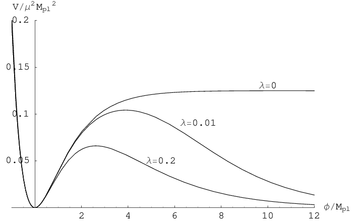
We will first explore the possibility that is the inflaton, then discuss other constraints from our knowledge about the early universe. Figure 3.4 summarizes our constraints.
3.4.1 inflation

The possibility that higher order corrections to the gravitational Lagrangian might be responsible for a de Sitter inflationary period was examined thoroughly early on in the inflationary game [234, 235]. For , the potential is very flat for large , which is perfect for inflation. This model and other related ideas were extensively studied in [168, 178, 119, 122, 80, 22], which also confirmed the existence of a viable inflationary model. We now search for possible inflationary scenarios with that are consistent with current observations. This question was already considered in [29], which found ; however, we wish to be more quantitative in light of the latest CMB measurements.
As usual in these models, it is important to keep careful track of whether we are working in the EF or the JF: recall that the potential is defined in the EF, while matter is most naturally considered in the JF. Nonetheless, we will argue that the inflationary predictions are exactly the same as those of general relativity plus a normal slow rolling scalar field with potential . The argument goes as follows. Slow roll inflation works normally in the EF where the graviton and scalar field have canonical actions. In particular, the EF is where one should calculate the spectrum of tensor and scalar mode fluctuations. Re-heating and the transformation of fluctuations in to adiabatic density fluctuations also works as usual in the EF, because at this time the cosmic fluid is relativistic and hence governed by the same equations of motion in both frames. After reheating, is frozen out at the minimum of , with and , so there is no longer any distinction between the JF and the EF (). Calculations for were performed both as above and in the JF in [119], and the results were found to be consistent as expected.
Using this idea, calculating the inflationary predictions is straightforward. Using Eq. (3.16), we can estimate the reheating temperature as , where is the number of minimally coupled scalar fields into which decays (it decays most strongly into these fields). Then the scale factor (normalized to today) is
| (3.59) |
at the end of inflation. Integrating the slow roll equations of motion, , and assuming , the number of -foldings of inflation for a mode is
| (3.60) |
Here is a small number defined such that at the end of inflation, where , and is related to the conformal factor when the mode crosses the horizon:
| (3.61) |
This particular mode will have a scalar fluctuation amplitude (also referred to as in the literature)
| (3.62) |
where the slow roll parameters (using the definitions in [24]) are
| (3.63) |
We then use these to find the the scalar spectral index , the ratio of tensor to scalar modes etc. Using the combined WMAP+SDSS measurements [242] for modes we can use Eq. (3.60-3.62) together to fix . For the result is
| (3.64) | |||||
| (3.65) | |||||
| (3.66) |
which is consistent with the both the theoretical results of [119, 178] and recent observational constraints [231, 242].
In addition, is sensitive to the value of . The observational constraint (68% C.L.) from [242], translates into a strong upper bound on :
| (3.67) |
This is an example of the usual fine tuning that is needed for observationally allowed inflationary potentials and is consistent with the findings of [29]. More precisely the values of appropriate for inflation are shown in Fig 3.4.
3.4.2 Other constraints
Above we explored the possibility that was the inflaton. Let us now turn to the alternative possibility that is not the inflaton, and compute miscellaneous constraints on the parameters and when they are varied freely. We will first consider the fifth force mediated by , then investigate how the scalar field behaves dynamically in the early universe, where the most interesting effect comes from considering a period of slow-roll inflation driven by some other scalar field. As noted in Section 3.2, the dynamics of is still governed by an effective potential Eq. (3.26) which is important when there is a component of matter whose energy-momentum tensor has nonzero trace.
To begin with, we ignore any effect that such a term may have on the minimum of for these polynomial models, which is a good approximation if . We will see that for the first few constraints that we derive, this will indeed be the case. Then we will return to the question of where this is a bad approximation, which will naturally lead to our discussion of slow-roll inflation by some other scalar field.
Fifth force constraints
The minimum of the effective potential lies at , . The curvature of this minimum is . Hence we can get around solar system constraints simply by making large enough so that the range of the fifth force will be small. Clearly it must have an range smaller than the solar system, otherwise, as was discussed above, it will violate the bound on the PPN parameter . (Recall that there is no Chameleon effect here, so in Eq. (3.42) and .) For smaller scales, we consider searches for a fifth force via deviations from the inverse square law. The profile for a quadratic potential, i.e, Eq. (3.31), gives a Yukawa potential between two tests masses and :
| (3.68) |
where . For this -value, a fifth force is ruled out for any Compton wavelength ranging from solar system scales down to , where the lower bound comes from the Eöt-Wash experiments [114]. This bound translates to
| (3.69) |
This implies , a typical solar system density, so for this constraint we were justified in ignoring any effects of the density-dependent term on the minimum of .
Nucleosynthesis constraints
Given this preliminary constraint from local gravity tests, let us now consider the cosmology of in the EF. We may approximate the potential around the minimum by a quadratic potential , which is valid for . The interesting behavior will come during the radiation dominated epoch, so in Eq. (3.23) we take , and we ignore the term in Eq. (3.24) to find the cosmological equations of motion
| (3.70) | |||||
| (3.71) |
where the primes denote . There are two interesting limiting behaviors, corresponding to and , which we will now explore in turn.
For , the friction term in Eq. (3.71) dominates, and is frozen out at some value with . The energy density of is subdominant in Eq. (3.70). Therefore, in the EF we have the usual radiation dominated expansion, and in the JF using Eq. (3.22) and Eq. (3.20) we have the same Friedmann-Robertson-Walker (FRW) expansion with a different effective Newton’s constant : , where
| (3.72) |
For , on the other hand, assuming , the field starts to oscillate with frequency and an amplitude that redshifts as . Hence in the EF, the energy density of in Eq. (3.70) from these zero momentum field oscillations is , where . Mapping back into the JF, and averaging over a cycle of this oscillation, we obtain the Friedmann equation
| (3.73) |
where the unusual factor of comes from the averaging of the oscillations of in Eq. (3.72), as is discussed in more depth in [2].
The crossover between these two behaviors occurs when is comparable to , and given the laboratory tests of gravity above we can say that this must occur when the universe has at least the temperature . We were therefore justified in assuming radiation domination in our calculation.
Let us examine further the zero momentum oscillations of that give this extra non-relativistic energy density. In the absence of some mechanism (such as an extra period of low scale inflation [212]), we expect the initial amplitude of oscillations to be of the order . This is because the potential in Figure 3.5 varies on the scale of independently of the height of . Hence in the absence of any other scale, the initial amplitude must be around this size. Recall that at the onset of oscillations, , so the initial energy density of these oscillations is
| (3.74) |
This energy density subsequently grows relative to the radiation density component, quickly forcing the universe into a matter dominated period of expansion. This is unacceptable if this component does not decay before the onset of BBN, because then at the time of BBN the expansion would be much faster than the normal radiation dominated expansion, which would be inconsistent with observed primordial abundances [66].
The fact that interacts weakly with other particles (the vertices in Eq. (3.16) are suppressed by ) so that decays too slowly is exactly what is known as the cosmological moduli problem. To be more precise, we can use Eq. (3.16) to estimate the decay rate of zero momentum modes into other massive particles:
| (3.75) |
where the sums are over minimally coupled scalar particles and fermions with masses . The requirement translates into the constraint for the Standard Model. One would expect the bound on to be slightly smaller if one includes other particles that have not been detected yet with mass smaller than . This constraint should not be taken too seriously, however, because the moduli problem may hypothetically be resolved by electroweak scale inflation [132] or even by a brief second period of inflation at the electroweak scale [212].
Density dependent forces
We now consider how the extra density dependent term in may effect cosmology. In other words, when can we not neglect the forcing term of Eq. (3.24)? After enters the oscillating phase when , the extra term has little effect on the minimum since then it is small compared to the size of the potential itself (). As a result, simply oscillates as expected. Before the crossover, when is frozen, we showed that the universe must be radiation dominated so that in particular, as during this phase, the Hubble friction will dominate compared to the force term of in Eq. (3.24), and we were justified in claiming that is frozen out. The cosmology here does not suffer from the instability that plagues Eq. (3.1).
There are, however, some exceptions that might lead to interesting constraints. First, consider a relativistic component of the cosmological plasma that becomes non-relativistic and dumps its energy into the other relativistic components. In this case, for a period of about one e-folding, so receives a kick and is displaced by an amount [45]. This might lead to an interesting effect such as being kicked out of the basin of attraction of . The extreme case would be that does not end up oscillating around the minimum as expected when , but instead ends up rolling down the tail of , an effect which is clearly only possible for . In principle, such kicks could even invalidate the predictions of BBN: near the onset of BBN, annihilation occurs, displacing and consequently changing significantly as per Eq. (3.72). However, we have already shown that must be in the oscillatory phase long before the onset of BBN, and we have argued that these kicks have no effect while is in the oscillator phase, so in fact this effect is unlikely to have relevance for BBN. Such kicks may effect other important cosmological dynamics at temperatures higher than , such as baryogenesis. However, the effects are extremely model dependent, and it is hard to say anything definitive at this point.
Non-inflation
Another situation when we cannot ignore the density dependent force on is during inflation. Here is large for many e-foldings. Remember that in this section, we are not considering as our inflaton; instead we consider a slow roll inflationary period driven by some other scalar field defined in the JF. We wish to examine the effect a modified gravity Lagrangian such as Eq. (3.56) has on the inflationary scenario. In particular, we will be interested in situations where inflation by the field does not work, being effectively sabotaged by . We will discuss the generality of these assumptions at the end.
Such models have been considered before in the context of both the models [95, 133, 51] and other generalized gravity models [30]. There the goal was generally to make the inflationary predictions more successful, focusing on working models.
In the JF, consider a scalar field with a potential . We assume that is slow rolling; . This is the assumption that
| (3.76) |
which must be checked for self-consistency once we have solved for . We can now easily calculate by first working in the EF and mapping back to the JF. The equations of motion in the EF, Eqs. (3.23-3.24), become
| (3.77) |
| (3.78) |
It is interesting that a constant vacuum term in the JF does not translate into to a constant term in the EF. See Figure 3.5 for some examples of the effective potential ; we see that for large enough , the minimum vanishes. One finds that there is no minimum of the effective potential for
| (3.79) |
In particular, there is always a minimum for .
The resulting behavior of the inflaton depends on the size of compared to .

For small , it is clear that there is a stable minimum around which will oscillate. In this situation, the effective potential has a minimum at with value approximately , so after the energy density of oscillations redshift away, we are left with an exponentially expanding universe with , and . Hence in the JF, gravity behaves as it normally would in general relativity: for a flat potential, the slow roll conditions are satisfied, and inflation driven by works as it normally would. This is the expected situation, and it will happen for .
On the other hand, we now show that when and when there is no minimum of the effective potential (), we get a contradiction to the assumption that was slow rolling. Hence we show that it is not possible for to drive slow-roll inflation. For large , the potential may be approximated as . We treat as a constant and find that there is an exact attractor solution to Eq. (3.77) of the form and . Mapping this into the EF, we find the behavior , i.e., a period of radiation dominated expansion analogous to the MDE of [10] More specifically, we find
| (3.80) |
This is clearly not an inflating universe. So the slow roll assumptions of Eq. (3.76) are not consistent in this case. We therefore conclude that it is not possible for to drive slow-roll inflation.
Instead, dumps most of its energy into radiation, and as before, is left frozen at some point until . After this, can either drive an inflationary period itself as in the original discussion of inflation, or if is not in the basin of attraction of , it will roll down the tail of . In neither situation has inflated our universe. From this combination of inflaton plus gravity with , we only get satisfactory inflation if lies in the region of parameter space appropriate for inflation (the blue/grey sliver in Figure 3.4) and if sits at a point which allows for the required number of e-foldings.
Gravitational wave constraints
It is well-known that inflation produces horizon-scale gravitational waves of amplitude , so that the energy scale of inflation can be bounded from above by the current observational upper limit [231, 242] and perhaps measured by a detection of the gravitational wave signal with future CMB experiments [38]. Using such a detection one might try to constrain by the arguments of the previous section. Specifically, by demanding that during inflation there is a minimum of the effective potential one can find a constraint by invoking Eq. (3.79) with (incorrectly) replaced by the measured energy density of inflation.
However, because of the EF-JF duality, one needs to carefully define what one means by “the energy scale of inflation”. The bound from the above argument simply precludes inflatons with a given energy density in the JF, but is merely a parameter which does not necessarily set the energy scale of inflation. In addition to this problem, we cannot use Eq. (3.79) to derive a constraint for , because in this case there is always a minimum in the effective potential and it is always possible for to slow roll (this situation is described in greater depth in [133, 95]).
To make these ideas more concrete and resolve both of these ambiguities, we will operationally define the energy scale of inflation to be the one that makes the standard GR formula for the gravitational wave amplitude valid. It is clear that the amplitude of gravitational waves should be calculated in the EF where the metric has a canonical action. The result is then passed trivially into the JF after inflation and when . The Hubble scale then sets the size of the fluctuations, but it is a complicated model dependent calculation to find exactly when the relevant fluctuations are generated. However, there is a limit to the size of for which the EF is approximately inflating, and so gravitational waves are being generated. Following the discussion above of non-working inflatons, we demand that must be slow rolling down the effective potential defined in Eq. (3.78) for both frames to be inflating. In this situation, both scalar and gravity modes are being generated.
The procedure is thus to find the maximum value of (that is, from Eq. (3.77), the maximum value of ) such that is slow rolling. We then maximize this with respect to the parameter to find the largest amplitude of gravitational waves that can possibly be produced. At each step in this procedure, we wish to be as conservative as possible; for example, we define slow roll through the slow roll parameter constraints and to allows for the possibility of power law inflation. Where again we use the standard defintion of and from [24].
As an example, consider the case. Here it is possible to show that for to be slow rolling, it must satisfy
| (3.81) |
where always lies to the left of the minimum of . The maximum Hubble scale in the EF for a given is then . This is maximized for large , with the result that where we have used Eq. (3.81). This translates into a constraint on the maximum gravitational wave amplitude that can be produced,
| (3.82) |
Given a measurement of the tensor to scalar ratio , this places a limit on :
| (3.83) |
Numerically, we find similar results for non-zero . We plot examples of this constraint in Figure 3.4, combined with the already discussed working inflationary models. Note that for a given , it is important that this constraint lies below the corresponding working inflationary model (the blue/grey thin sliver of Fig. 3.4) with the same ; fortunately, as is indicated by the arrows in this figure, it does.
If gravitational waves are not detected, then this argument gives no lower bound on . In particular, it is possible that inflation occurred at the electroweak scale, in which case the constraint is the best we can do.
Note that we completely ignore the production of scalar fluctuation modes for this argument. This is because the scalar modes are much more difficult to calculate, since there are two scalar fields in the mix, and , which are canonically defined in different frames. But the scalar modes are also model dependent and one should generally be able to fine tune to give the correct amplitude and spectral index without affecting the above argument. This more complicated problem was considered for chaotic inflation with gravity in [51].
This constraint applies only to slow-roll inflation models. There are classes of fast-roll inflation, but these models have problems of their own and generally fail to reproduce the required scale invariance (see [147] for a review).
Finally, let us discuss some inflaton models that might circumvent this constraint. It is possible to add an inflaton in the EF. However, this theory is then not conformally equivalent to an theory: the two scalar fields and get mixed up. Hence it is not in the class of models we set out to constrain. Another possibility is to add an inflaton which is conformally coupled to gravity and has a potential. This does not change from frame to frame and so inflation might be expected to work. However, it was shown by [136] that non-minimally coupled scalar fields cannot drive inflation.
In any case, if gravitational waves are found, then this constraint must be thought about seriously when using such models in other astrophysical or local gravity situations.
3.5 Conclusions
We have searched for viable theories using the wealth of knowledge on scalar tensor theories to which theories are equivalent. We studied two classes of models: the Chameleon and massive theories, which may well be the only classes of models that can be made consistent with local gravity observations.
The Chameleon that was studied is a special kind of scalar field which hides itself from solar system tests of gravity using non-linear effects associated with the all-important density-dependent effective potential. It was shown that, despite this Chameleon behavior, solar system tests still preclude the possibility of observably dynamical DE; the best we could do was for the effective DE equation of state parameter relevant for the dynamics of the expansion. There are of course interesting effects of the Chameleon both for local gravity [127] and on cosmological density perturbations [44], and these may be worth future studies in the context of theories.
The massive theories were found to be more relevant for very high energy cosmology, so the conclusions were more speculative. First, the scalar field may be the inflaton, in which case we found the required polynomial to be quite fine tuned as is usual for inflationary potentials. If the scalar field was not the inflaton, then we saw that possible instabilities could spoil both inflation and Big Bang nucleosynthesis, giving interesting constraints on the shape of . If primordial gravitational waves are detected using the CMB, then the most naive models of inflation have serious problems unless the mass of the -scalar is very large; a measured scalar to tensor ratio of requires . If gravitational waves are not found, then the best we can say comes from the Eöt-Wash laboratory experiments constraining the extent of a 5th force: .
General relativity adorned with nothing but a cosmological constant, i.e., , is a remarkable successful theory. As we have discussed, a host of observational data probing scales from m to m not only agree beautifully with GR, but also place sharp constraints on the parametrized departures from GR that we have explored. In particular, both viable classes of theories that we studied were found to have no relevance for dynamic dark energy that is observationally distinguishable from “vanilla” dark energy, i.e., a cosmological constant. Since we have no good reason to believe that there are additional viable classes of -theories, it appears likely that no viable theories can produce the sort of interesting non-vanilla dark energy that many observers are hoping to find. However, without a much larger study of the parameter space (which is of course incredibly large) we shy away from making a stronger statement here.
We would like to thank Serkan Cabi, Alan Guth, Robert Wagoner and Matias Zaldarriaga for helpful discussion.
Chapter 4 Constraining cosmological parameters with 21cm tomography
4.1 Introduction
Three-dimensional mapping of our Universe using the redshifted 21 cm hydrogen line has recently emerged as a promising cosmological probe, with arguably greater long-term potential than the cosmic microwave background (CMB). The information garnered about cosmological parameters grows with the volume mapped, so the ultimate goal for the cosmology community is to map our entire horizon volume, the region from which light has had time to reach us during the 14 billion years since our Big Bang. Figure 4.1 illustrates that whereas the CMB mainly probes a thin shell from , and current large-scale structure probes (like galaxy clustering, gravitational lensing, type Ia supernovae and the Lyman forest) only map small volume fractions nearby, neutral hydrogen tomography is able to map most of our horizon volume.

| Assumptions | Pessimistic | Middle | Optimistic | |
| Power modeling | Ionization power spectrum modeling | Marginalize over arbitrary and | Marginalize over constants that parametrize and | No ionization power spectrum, . |
| Non-linear cut-off scale | ||||
| Non-Gaussianity of ionization signals | Doubles sample variance | Negligible | ||
| Cosmological | Reionization history | Gradual reionization over wide range of redshifts | Abrupt reionization at | |
| Redshift range | 7.3-8.2 | 6.8 - 10 | ||
| Parameter space | Vanilla model plus optional parameters | Vanilla model parameters | ||
| Experimental | Data | MWA, LOFAR, 21CMA | Intermediate case | SKA, FFTT |
| Array configuration 11 1 For the FFTT, we consider only the case where all dipoles are in a giant core. | , | Giant core | ||
| Collecting area 22 2 See designed or assumed values of in Table 4.4. | design values | Design values | Design values | |
| Observation time 33 3 Assumes observation of two places in the sky. | ||||
| System temperature | in [41] | given in [41] | in [41] | |
| Astrophysical | Residual foregrounds cut-off scale 44 4 It is hard to predict the level of the residual foregrounds after the removal procedure. To quantify contributions from other factors, we take the approximation that there is no residual foregrounds at . Here in the table, is the comoving (l.o.s.) distance width of a single -bin. | |||
| Vanilla Alone | ||||||||||||||
| 55 5 refers to the mean neutral fraction at redshift . | [eV] | |||||||||||||
| Planck | 0.0070 | 0.0081 | 0.0059 | 0.0033 | 0.0088 | 0.0043 | … | … | … | … | 0.025 | 0.23 | 0.0026 | |
| All OPT | 0.0044 | 0.0052 | 0.0051 | 0.0018 | 0.0087 | 0.0042 | 0.0063 | 0.0063 | 0.0063 | 0.0063 | 0.0022 | 0.023 | 0.00073 | |
| +LOFAR | All MID | 0.0070 | 0.0081 | 0.0059 | 0.0032 | 0.0088 | 0.0043 | 0.18 | 0.26 | 0.23 | … | 0.018 | 0.22 | 0.0026 |
| All PESS | 0.0070 | 0.0081 | 0.0059 | 0.0033 | 0.0088 | 0.0043 | … | 51 | 49 | … | 0.025 | 0.23 | 0.0026 | |
| All OPT | 0.0063 | 0.0074 | 0.0055 | 0.0024 | 0.0087 | 0.0043 | 0.0062 | 0.0062 | 0.0062 | 0.0062 | 0.0056 | 0.017 | 0.00054 | |
| +MWA | All MID | 0.0061 | 0.0070 | 0.0056 | 0.0030 | 0.0087 | 0.0043 | 0.32 | 0.22 | 0.29 | … | 0.021 | 0.19 | 0.0026 |
| All PESS | 0.0070 | 0.0081 | 0.0059 | 0.0033 | 0.0088 | 0.0043 | … | 29 | 30 | … | 0.025 | 0.23 | 0.0026 | |
| All OPT | 0.00052 | 0.0018 | 0.0040 | 0.00039 | 0.0087 | 0.0042 | 0.0059 | 0.0059 | 0.0059 | 0.0059 | 0.0011 | 0.010 | 0.00027 | |
| +SKA | All MID | 0.0036 | 0.0040 | 0.0044 | 0.0025 | 0.0087 | 0.0043 | 0.0094 | 0.014 | 0.011 | … | 0.0039 | 0.056 | 0.0022 |
| All PESS | 0.0070 | 0.0081 | 0.0059 | 0.0033 | 0.0088 | 0.0043 | … | 1.1 | 1.0 | … | 0.025 | 0.23 | 0.0026 | |
| All OPT | 0.00010 | 0.0010 | 0.0029 | 0.000088 | 0.0086 | 0.0042 | 0.0051 | 0.0051 | 0.0051 | 0.0051 | 0.00020 | 0.0018 | 0.000054 | |
| +FFTT66 6 FFTT stands for Fast Fourier Transform Telescope, a future square kilometer array optimized for 21 cm tomography as described in [245]. Dipoles in FFTT are all in a giant core, and this configuration does not vary. | All MID | 0.00038 | 0.00034 | 0.00059 | 0.00033 | 0.0086 | 0.0042 | 0.0013 | 0.0022 | 0.0031 | … | 0.00023 | 0.0066 | 0.00017 |
| All PESS | 0.0070 | 0.0081 | 0.0059 | 0.0033 | 0.0088 | 0.0043 | … | 0.0043 | 0.0047 | … | 0.025 | 0.11 | 0.0024 | |
Several recent studies have forecast the precision with which such 21 cm tomography can constrain cosmological parameters, both by mapping diffuse hydrogen before and during the reionization epoch [159, 40, 218] and by mapping neutral hydrogen in galactic halos after reionization [270]. These studies find that constraints based on the cosmic microwave background measurements can be significantly improved. However, all of these papers make various assumptions, and it is important to quantify to what extent their forecasts depend on these assumptions. This issue is timely because 21 cm experiments (like LOFAR [148], 21CMA [1], MWA [182] and SKA [226]) are still largely in their planning, design or construction phases. These experiments will be described in detail in Section 4.2.7. In order to maximize their scientific “bang for the buck”, it is therefore important to quantify how various design tradeoffs affect their sensitivity to cosmological parameters.
The reason that neutral hydrogen allows mapping in three rather than two dimensions is that the redshift of the cm line provides the radial coordinate along the line-of-sight (l.o.s.). This signal can be observed from the so-called dark ages [224, 143] before any stars had formed, through the epoch of reionization (EoR), and even to the current epoch (where most of the neutral hydrogen is confined within galaxies). We focus in this study on the cm signal from – the end of the dark ages through the EoR. This is the redshift range at which the synchrotron foregrounds are smallest, and consequently is the range most assessable for all planned cm arrays.
There are three position-dependent quantities that imprint signatures on the 21 cm signal: the hydrogen density, the neutral fraction, and the spin temperature. For cosmological parameter measurements, only the first quantity is of interest, and the last two are nuisances. (For some astronomical questions, the situation is reversed.) The 21 cm spin-flip transition of neutral hydrogen can be observed in the form of either an absorption line or an emission line against the CMB blackbody spectrum, depending on whether the spin temperature is lower or higher than the CMB temperature.
During the epoch of reionization, the spin temperature is likely coupled to the gas temperature through Ly photons via the Wouthuysen-Field Effect [269, 87], and the gas in the IGM has been heated by X-ray photons to hundreds of Kelvin from the first stars [208]. If this is true, the 21cm signal will only depend on the hydrogen density and the neutral fraction. However, astrophysical uncertainties prevent a precise prediction for exactly when the gas is heated to well above the CMB temperature and is coupled to the spin temperature. In this chapter, we follow [159, 40] and focus entirely on the regime when the spin temperature is much larger than the CMB temperature [276, 93, 217], such that the observed signal depends only on fluctuations in density and/or the neutral fraction. Specifically, we focus on the time interval from when this approximation becomes valid (around the beginning of the reionization [276, 93, 217]) until most hydrogen has become ionized, illustrated by the darkest region in Figure 4.1. Despite this simplification, the methods that we apply to model the ionization fluctuations almost certainly can be applied to model spin temperature fluctuations with minimal additional free parameters.
In Table 4.1, we list all the assumptions that affect the accuracy of cosmological parameter measurements, including ones about power modeling, cosmology, experimental design, and astrophysical foregrounds. For each case, we provide three categories of assumptions: one pessimistic (PESS), one middle-of-the-road (MID) and one optimistic (OPT). Since we wish to span the entire range of uncertainties, we have made both the PESS and OPT models rather extreme. The MID model is intended to be fairly realistic, but somewhat on the conservative (pessimistic) side.
Before describing these assumptions in detail in the next section, it is important to note that taken together, they make a huge difference. Table 4.2 illustrates this by showing the cosmological parameter constraints resulting from using all the OPT assumptions, all the MID assumptions or all the PESS assumptions, respectively. For example, combining CMB data from Planck and 21 cm data from FFTT, the uncertainty differs by a factor of 125 for and by a factor of 78 for depending on assumptions. It is therefore important to sort out which of the assumptions contribute the most to these big discrepancies, and which assumptions do not matter much. This is a key goal of our chapter.
The rest of this chapter is organized as follows. In Section 4.2, we explain in detail the assumptions in the same order as in Table 4.1, and also present a new method for modeling the ionization power spectra. In Section 4.3, we quantify how the cosmological parameter measurement accuracy depends on each assumption, and we derive simple analytic approximations of these relations. In Section 4.4, we conclude with a discussion of the relative importance of these assumptions, and implications for experimental design.
4.2 Forecasting Methods & Assumptions
4.2.1 Fundamentals of 21cm cosmology
Power spectrum of 21 cm radiation
We review the basics of the 21 cm radiation temperature and power spectrum only briefly here, and refer the interested reader to [92] for a more comprehensive discussion of the relevant physics. The difference between the observed 21 cm brightness temperature at the redshifted frequency and the CMB temperature is [88]
| (4.1) |
where is the spin temperature, is the number density of the neutral hydrogen gas, and s-1 is the spontaneous decay rate of 21cm transition. The factor is the gradient of the physical velocity along the line of sight ( is the comoving distance), which is on average (i.e. for no peculiar velocity). Here is the Hubble parameter at redshift . The spatially averaged brightness temperature at redshift is (in units of )
| (4.2) |
where is the mean neutral fraction, and is the averaged spin temperature. If in the EoR, the 21cm emission should therefore be observed at the level of milli-Kelvins.
To calculate the fluctuations, we rewrite Eq. (4.1) in terms of (the hydrogen mass density fluctuation), (the fluctuation in the ionized fraction), and the gradient of the peculiar velocity along the line of sight, using the fact that :
| (4.3) |
Here is the mean ionized fraction, and we have defined . We write . In Fourier space, it is straightforward to show that, as long as so that linear perturbation theory is valid, , where is the cosine of the angle between the Fourier vector and the line of sight. In this chapter, we restrict our attention to the linear regime. We will also throughout this chapter assume during the EoR, making the last factor in Eq. (4.3) unity for the reasons detailed in Section 4.1.
In Fourier space, the power spectrum of the 21cm fluctuations is defined by , where is the deviation from the mean brightness temperature. It is straightforward to show from Eq. (4.3) that, to leading order,
| (4.4) |
Here and are the ionization power spectrum and the density-ionization power spectrum respectively. For convenience, we define , and , so the total 21 cm power spectrum can be written as three terms with different angular dependence:
| (4.5) |
where
| (4.6) | |||||
| (4.7) | |||||
| (4.8) |
Since involves only the matter power spectrum that depends only on cosmology, Barkana and Loeb [19] argued that in principle, one can separate cosmology from astrophysical “contaminants” such as and whose physics is hitherto far from known. We will quantify the accuracy of this conservative approach (which corresponds to our PESS scenario for ionization power spectrum modeling below) in Section 4.3.
From to
The power spectrum and the comoving vector (the Fourier dual of the comoving position vector ) are not directly measured by 21cm experiments. An experiment cannot directly determine which position vector a signal is coming from, but instead which vector it is coming from, where give the angular location on the sky plane, and is the frequency difference from the central redshift of a -bin. For simplicity, we assume that the sky volume observed is small enough that we can linearize the relation between and . Specifically, we assume that the sky patch observed is much less than a radian across, so that we can approximate the sky as flat 77 7 The FFTT is designed for all-sky mapping (i.e. the field of view is of order ). However, since the angular scales from which we get essentially all our cosmological information are much smaller than a radian (with most information being on arcminute scales), the flat-sky approximation is accurate as long as the data is analyzed separately in many small patches and the constraints are subsequently combined., and that separations in frequency near the mean redshift are approximately proportional to separations in comoving distance. In these approximations, if there are no peculiar velocities,
| (4.9) | |||||
| (4.10) |
Here “” denotes the vector component perpendicular to the line of sight, i.e., in the -plane, and is the comoving angular diameter distance given by [135]
| (4.11) |
where
| (4.12) |
is the relative cosmic expansion rate and the function equals if , if , and if . The conversion factor between comoving distances intervals and frequency intervals is
| (4.13) |
where cm is the rest-frame wavelength of the 21 cm line.
We write the Fourier dual of as ( has units of time). The relation between and is therefore
| (4.14) | |||||
| (4.15) |
In -space, the power spectrum of 21cm signals is defined by , and is therefore related to by
| (4.16) |
Note that cosmological parameters affect in two ways: they both change and alter the geometric projection from -space to -space. If and changed while remained fixed, the observable power spectrum would be dilated in both the and directions and rescaled in amplitude, while retaining its shape. Since both and depend on the three parameters , and the Hubble parameter is in turn given by the parameters in Table 4.2 via the identity , we see that these geometric effects provide information only about our parameters . Baryon acoustic oscillations in the power spectrum provide a powerful “standard ruler”, and the equations above show that if one generalizes to the dark energy to make an arbitrary function of , then the cosmic expansion history can be measured separately at each redshift bin, as explored in [270, 156, 59]. 21 cm tomography information on our other cosmological parameters (, , , , , etc.) thus comes only from their direct effect on . Also note that affect only by modulating the rate of linear perturbation growth, so they alter only the amplitude and not the shape of .
If we were to use Eq. (4.16) to infer from the measured power spectrum while assuming incorrect cosmological parameter values, then this geometric scaling would cause the inferred to be distorted by the so-called Alcock-Paczyński (AP) effect [189, 18] and not take the simple form of Eqns.(4.5)-(4.8). To avoid this complication, we therefore perform our Fisher matrix analysis directly in terms of , since this quantity is directly measurable without any cosmological assumptions.
The above transformations between -space and -space are valid when there are no peculiar velocities. The radial peculiar velocities that are present in the real world induce the familiar redshift space distortions that were discussed in Section 4.2.1, causing and power spectrum anisotropies that were described there.
4.2.2 Assumptions about and
During the EoR, ionized bubbles (HII regions) in the IGM grow and eventually merge with one another. Consequently, (k) and (k) contribute significantly to the total 21cm power spectrum. The study of the forms of these two ionization power spectra has made rapid progress recently, particularly through the semi-analytical calculations [93, 276, 157, 274] and radiative transfer simulations [158, 275]. However, these models depend on theoretically presumed parameters whose values cannot currently be calculated from first principles. From the experimental point of view, it is therefore important to develop data analysis methods that depend only on the most generic features of the ionization power spectra. In this chapter, we consider three methods — our OPT, MID and PESS models — that model and as follows:
| (4.17) |
| (4.18) |
| (4.19) |
In the next three subsections, we explain these models in turn.
OPT model
It is likely that before reionization started (while and ), hydrogen gas had already been sufficiently heated that . In this regime, Eq. (4.17) holds. This OPT scenario is clearly the simplest model, since the total 21cm power spectrum is simply proportional to : . To forecast the error, we use the Fisher matrix formalism [243]. Repeating the derivation in [238], the Fisher matrix for cosmological parameters () is
| (4.20) |
where the integral is taken over the observed part of -space, and denotes the combined power spectrum from cosmological signal and all forms of noise. Here is the volume of the -space where is the solid angle within the field of view (f.o.v.) and is the frequency size of a -bin. The Fisher matrix determines the parameter errors as .
For computational convenience, we subdivide -space into pixels so small that the power spectrum is roughly constant in each one, obtaining
| (4.21) |
where the power spectrum measurement error in a pixel at is
| (4.22) |
Here is the noise power spectrum and will be discussed in detail in Section 4.2.7; note that it is independent of and depends only on through the baseline distribution of the antenna array.
| (4.23) |
is the number of independent cells in an annulus summing over the azimuthal angle. We have the factor in instead of the normal because we only sum over half the sphere.
| 9.2 | 0.9 | 0.208 | 1.24 | -1.63 | 0.38 | 0.45 | 0.56 | -0.4 |
|---|---|---|---|---|---|---|---|---|
| 8.0 | 0.7 | 2.12 | 1.63 | -0.1 | 1.35 | 1.47 | 0.62 | 0.46 |
| 7.5 | 0.5 | 9.9 | 1.3 | 1.6 | 2.3 | 3.1 | 0.58 | 2. |
| 7.0 | 0.3 | 77. | 3.0 | 4.5 | 2.05 | 8.2 | 0.143 | 28. |
MID model
After reionization starts, both ionization power spectra and make significant contribution to the total 21cm power spectrum. We explore two different analysis methods — our MID and PESS models — for separating the cosmological signal from these astrophysical contaminants (i.e. and ).
Our MID model assumes that both ionization power spectra and are smooth functions of which can be parametrized by a small number of nuisance parameters related to reionization physics. Combining these ionization parameters with our cosmological ones into a larger parameter set (), we can jointly constrain them by measuring .
In Appendix 4.A we will describe a goodness-of-fit test for quantifying whether this parametrization is valid. The Fisher matrix for measuring is simply
| (4.24) |
This Fisher matrix is not block diagonal, i.e., there are correlations between the cosmological and ionization parameters, reflecting the fact that both affect and . The inversion of the Fisher matrix therefore leads to the degradation of the constraints of cosmological parameters. However, the total 21cm power spectrum is usually smaller in magnitude in the MID model than in the OPT model (see Eq. (4.4)), giving less sample variance. This means that as long as noise in a 21cm experiment dominates over sample variance, the MID model will give weaker constraints than the OPT model, because of the degeneracies. For future experiments with very low noise, however, it is possible to have the opposite situation, if the reduction in sample variance dominates over the increase in degeneracy. This does of course not mean that the MID model is more optimistic than the OPT model, merely that the OPT model is assuming an unrealistic power spectrum.
Having set up the general formalism, we now propose the specific parametrization specified by Eq. (4.18), with fiducial values of ionization parameters given in Table 4.3. This parametrization was designed to match the results of the radiative transfer simulations in Model I of [158], and Figure 4.2 shows that the fit is rather good in the range to which the 21cm experiments we consider are most sensitive.
The radiative transfer simulations implemented in [158] are post processed on top of a N-body simulation in a box of size . Three models for the reionization history are considered in [158]:
- 1.
In Model I, all dark matter halos above (corresponding to the minimum mass galaxy in which the gas can cool by atomic transitions and form stars, e.g. at ) contribute ionizing photons at a rate that is proportional to their mass.
- 2.
In Model II, the ionizing luminosity of the sources scales as halo mass to the power, i.e. more massive halos dominate the production of ionizing photons than in Model I.
- 3.
In Model III, which has the same source parametrization as in Model I except for doubled luminosity, minihalos with absorb incident ionizing photons out to their virial radius unless they are photo-evaporated (but do not contribute ionizing photons).
It appears to be a generic feature in the simulation results that the ratios of functions at large fall off like a power law for , and exponentially for . At small , can either increase or decrease approximately linearly as increases, while is asymptotically constant. Our parametrization in Eq. (4.18) captures these features: at large , and ; at small , , and (both and can be either positive or negative). Figure 4.2 also shows that for and also for at large , our parametrization further improves over the parametrization suggested by Santos and Cooray [218], which works well for at small .
To be conservative, we discard cosmological information from and in our Fisher matrix analysis by using the fiducial power spectrum rather than the actual one in Eq. (4.18). This means that the derivatives of and with respect to the cosmological parameters vanish in Eq. (4.24). It is likely that we can do better in the future: once the relation between the ionization power spectra and the matter power spectrum can be reliably calculated either analytically or numerically, the ionization power spectra can contribute to further constraining cosmology.
In addition to the fit of Model I shown in Figure 4.2, we also fit our model (with different fiducial values from those listed in Table 4.3) to the simulations using Model II and III in [158], and find that the parametrization is flexible enough to provide good fits to all three simulations, suggesting that the parametrization in Eq. (4.18) may be generically valid and independent of models. Note, however, that at low redshifts (), our parametrization of does not work well at large , in that the simulation falls off less rapidly than exponentially. This may be because when HII regions dominate the IGM, the ionized bubbles overlap in complicated patterns and correlate extremely non-linearly at small scales. This partial incompatibility indicates that our parametrization (i.e. Eq.4.18) is only accurate for small , i.e. before non-linear ionization patterns come into play.
In the remainder of this chapter, we will adopt the values in Table 4.3 as fiducial values of the ionization parameters.
PESS model
By parametrizing the ionization power spectra with a small number of constants, the MID model rests on our understanding of the physics of reionization. From the point of view of a maximally cautious experimentalist, however, constraints on cosmological parameters should not depend on how well one models reionization. In this spirit, Barkana and Loeb [19] proposed what we adopt as our “PESS” model for separating the physics from the “gastrophysics” and . Instead of assuming a specific parametrization, the PESS model makes no a priori assumptions about the ionization power spectra. In each -bin that contains more than three pixels in -space, one can in principle separate from the other two moments. The PESS model essentially only constrains cosmology from the term and therefore loses all information in and . We now set up the Fisher matrix formalism for the PESS model that takes advantage of the anisotropy in arising from the velocity field effect. Numerical evaluations will be performed in Section 4.3.1.
The observable in 21cm tomography is the brightness temperature . In Fourier space, the covariance matrix between two pixels and is , assuming that the measurements in two different pixels are uncorrelated88 8 We ignore here a -function centered at the origin since 21cm experiments will not measure any modes.. The total 21cm power spectrum is . For convenience, we use the shorthand notation , where , and and define the for , respectively. Thus the power spectrum can be rewritten as . Treating at each -bin as parameters, the derivatives of the covariance matrix are simply , where resides in the shell of radius with width . Since the different -bins all decouple, the Fisher matrix for measuring the moments is simply a separate -matrix for each -bin:
| (4.25) | |||||
where . Here is related to by Eq. (4.16). Again the sum is over the upper half of the spherical shell . The error of is . Once is separated from other moments, can be used to constrain cosmological parameters with the Fisher matrix as given in Eq. (4.21).
We have hitherto discussed the anisotropy in that arises from the velocity field effect. However, the AP-effect may further contribute to the anisotropy in that it creates a -dependence and modifies the term [189, 18]. The AP-effect can be distinguished from the velocity field effect since the term is unique to the AP-effect. Thus, one can constrain cosmological parameters from and [159], involving the inversion of a matrix which loses even more information and therefore further weakens constraints. Therefore, the PESS Fisher matrix that we have derived without taking AP-effect into account can be viewed as an upper bound on how well the PESS approach can do in terms of cosmological parameter constraints. However, this maximally conservative matrix approach may be inappropriately pessimistic, since the AP-induced clustering anisotropy is typically very small within the observationally allowed cosmological parameter range, whereas the velocity-induced anisotropies can be of order unity.
4.2.3 Assumptions about Linearity
To avoid fitting to modes where is non-linear and physical modeling is less reliable, we impose a sharp cut-off at and exclude all information for . We take for our MID model, and investigate the -dependence of cosmological parameter constraints in Section 4.3.2.
4.2.4 Assumptions about non-Gaussianity
Non-Gaussianity of ionization signals generically becomes important at high . With a large volume, high resolution simulations of cosmic reionization, Lidz et al. [146] and Santos et al. [216] found non-negligible (a factor of 1.5) differences in the full power spectrum at high (). To get a rough sense of the impact of non-Gaussianity on cosmological parameter constraints, we simply model it as increasing the sample variance by a factor . We thus write the total power spectrum as
| (4.26) |
where is the factor by which the the sample variance is increased. The parameter should take the value (Gaussian) at epochs with low and (non-Gaussian) at high .
4.2.5 Assumptions about reionization history and redshift range
21cm tomography can probe a wide range of redshifts, as illustrated in Figure 4.1. However, one clearly cannot simply measure a single power spectrum for the entire volume, as the clustering evolves with cosmic time: The matter power spectrum changes gradually due to the linear growth of perturbations [244]. More importantly, the ionization power spectra vary dramatically with redshift through the epoch of reionization. We incorporate these complications by performing our analysis separately in a series of redshift slices, each chosen to be narrow enough that the matter and ionization power spectra can be approximated as constraint within each slice. This dictates that for a given assumed reionization history, thinner redshift slices must be used around redshifts where varies dramatically.
In this chapter, we will consider two rather opposite toy models in Section 4.3:
- •
OPT: A sharp reionization that begins and finishes at one redshift (say ).
- •
MID/PESS: A gradual reionization that spanning a range of redshifts, assuming the ionization parameter values that fit Model I simulation of the McQuinn et al. paper [158]
For the latter scenario, the ionization fraction is not a linear function of redshift. For example, in in the McQuinn et al. [158] simulation, 0.9, 0.7, 0.5 and 0.3 correspond to redshifts , 8.0, 7.5 and 7.0, respectively. For our different scenarios, we therefore adopt the redshift ranges that are divided into four redshift slices centered at the above redshifts (OPT), split into three bins centered at =7.0, 7.5 and 8.0 (MID), split into two slices centered at and 8.0.
4.2.6 Assumptions about cosmological parameter space
Since the impact of the choice of cosmological parameter space and related degeneracies has been extensively studied in the literature, we will perform only a basic analysis of this here. We work within the context of standard inflationary cosmology with adiabatic perturbations, and parametrize cosmological models in terms of 12 parameters (see, e.g. , Table 2 in [242] for explicit definitions) whose fiducial values are assumed as follows: (spatial curvature), (dark energy density), (baryon density), (Hubble parameter ), (reionization optical depth), (massive neutrino density), (scalar spectral index), (scalar fluctuation amplitude), (tensor-to-scalar ratio), (running of spectral index), (tensor spectral index) and (dark energy equation of state). We will frequently use the term “vanilla” to refer to the minimal model space parametrized by combined with and ionization parameters at all observed -bins, setting , and fixed at their fiducial values.
| Experiment | Min. baseline (m) | f.o.v. () | (m2) at z=6/8/1299 9 We assume that the effective collecting area is proportional to such that the sensitivity ( in ) meets the design specification. | |
| MWA | 500 | 4 | 9/14/18 | |
| SKA | 7000 | 10 | 30/50/104 | |
| LOFAR | 77 | 100 | 397/656/1369 | |
| FFTT | 1 | 1/1/1 |
4.2.7 Assumptions about Data
The MWA, LOFAR, SKA and FFTT instruments are still in their planning/design/development stages. In this chapter, we adopt the key design parameters from [41] for MWA, [220] and www.skatelescope.org for SKA, www.lofar.org for LOFAR, and [245] for FFTT unless explicitly stated.
Interferometers
We assume that MWA will have 500 correlated antenna tiles, each with 16 dipoles. Each individual tile will have an effective collecting area of at and at . LOFAR will have 77 large (diameter stations, each with thousands of dipole antennae such that it has the collecting area nearly 50 times larger than each antenna tile of MWA. Each station can simultaneously image regions in the sky. We set in this chapter but this number may be larger for the real array. The design of SKA has not been finalized. We assume the “smaller antennae” version of SKA, in which SKA will have 7000 small antennae, much like MWA, but each panel with much larger collecting area. FFTT stands for Fast Fourier Transform Telescope, a future square kilometer array optimized for 21 cm tomography as described in [245]. Unlike the other interferometers we consider, which add in phase the dipoles in each panel or station, FFTT correlates all of its dipoles, resulting in more information. We evaluate the case where FFTT contains a million dipole antennae in a contiguous core subtending a square kilometer, providing a field-of-view of steradians.
For all interferometers, we assume that the collecting area , like a simple dipole, except that is saturated at in MWA since the wavelength exceeds the physical radius of an MWA antenna panel. The summary of the detailed specifications adopted in this chapter is listed in Table 4.4.
Configuration
The planned configurations of the above-mentioned interferometers are quite varied. However, all involve some combination of the following elements, which we will explore in out calculations:
- 1.
A nucleus of radius within which the area coverage fraction is close to 100%.
- 2.
A core extending from radius our to where there coverage density drops like some power law .
- 3.
An annulus extending from to where the coverage density is low but rather uniform.
In its currently planned design, the MWA will have a small () nucleus, while the core density falls off as until a sharp cutoff at m. For LOFAR we assume 32 stations in a core of radius , and another 32 stations in an outer annulus out to radius . For SKA we assume 20% in the core, and 30% in the annulus out to radius . We ignore the measurements from any dilute distribution of antenna panels outside . For LOFAR and SKA, we assume a uniform distribution of antennae in the annulus, but with an inner core profile like that of the MWA, i.e., a nucleus of radius (LOFAR/SKA) and an fall-off outside this compact core. We assume an azimuthally symmetric distribution of baselines in all arrays.
For an array with antennae within , we can define a quantity
| (4.27) |
where is the area density of the nucleus. is the maximal radius of the nucleus, corresponding to the case where there it contains all the antennae and there is no core.
It is also convenient to parametrize the distribution of these antennae within by two numbers: the fraction that are in the nucleus, and the fall-off index of the core. It is straightforward to show that and are related to and by
| (4.28) |
| (4.29) |
if . The analytic relation for is , which can be well approximated in numerical calculation by by taking in Eq. (4.29) with .

In Section 4.3.5, we will scan almost all possible design configurations and find the optimal one for constraining cosmology. There are two independent ways to vary array configurations, as illustrated by Figure 4.3: by varying with fixed, and by varying with fixed. Contributions from antennae in the annulus are negligible compared to the core, so varying is not interesting.
In other parts of Section 4.3, we will assume the intermediate configuration and (except for FFTT which is purely in a giant core) with the planned number of antennae in the core and annulus. Note that this configuration is optimized from the currently planned design.
Detector noise
21cm radio interferometers measure visibility . The visibility for a pair of antennae is defined as [176]
| (4.30) |
where are the number of wavelengths between the antennae. The hydrogen 3D map is the Fourier transform in the frequency direction where . The detector noise covariance matrix for an interferometer is [175, 159]
| (4.31) |
where is the frequency bin size, is system temperature, and is the observation time for the visibility at . Here is the total observation time, and is the number of baselines in an observing cell.
The covariance matrix of the 21cm signal is related to the power spectrum by [159]
| (4.32) | |||||
Therefore, the noise in the power spectrum is
| (4.33) |
For all interferometers, the system temperature is dominated by sky temperature due to synchrotron radiation in reasonable clean parts of the sky. Following [41], we set at and at .
4.2.8 Assumptions about Residual Foregrounds
There have been a number of papers discussing foreground removal for 21 cm tomography (e.g. [257, 74, 192, 75] and references therein), and much work remains to be done on this important subject, as the the amplitudes of residual foregrounds depend strongly depends on cleaning techniques and assumptions, and can have potentially dominate the cosmological signal. The work of Wang et al. [257] and McQuinn et al. [159] suggested that after fitting out a low-order polynomial from the frequency dependence in each pixel, the residual foregrounds were negligible for where is the comoving width of a -bin. To obtain a crude indication of the impact of residual foregrounds, there therefore we adopt the rough approximation that all data below some cutoff value is destroyed by foregrounds while the remainder has negligible contamination. We choose for the OPT/MID/PESS scenarios, and also explore wider ranges below.
4.3 Results and discussion
In this section, we numerically evaluate how the accuracy of cosmological parameter constraints depend on the various assumptions listed above. Where possible, we attempt to provide intuition for these dependences with simple analytical approximations. In most cases, we explore the dependence on one assumption at a time by evaluating the PESS, MID and OPT scenario for this assumption while keeping all other assumptions fixed to the baseline MID scenario.
4.3.1 Varying ionization power spectrum modeling and reionization histories
| Vanilla Alone | |||||||||||||
| Model | 1010 10 denotes the mean neutral fraction at the central redshift . ’s and are completely degenerate from the 21cm measurement alone. For this reason, the errors shown for from 21cm data alone is really not marginalized over ’s. | [eV] | |||||||||||
| LOFAR | OPT | 0.025 | 0.27 | 0.44 | 0.063 | 0.89 | … | … | … | … | 0.14 | 0.87 | 0.027 |
| MID | 0.13 | 0.083 | 0.15 | 0.36 | 0.80 | … | … | … | … | 0.35 | 12 | 0.17 | |
| MWA | OPT | 0.046 | 0.11 | 0.19 | 0.022 | 0.37 | … | … | … | … | 0.056 | 0.38 | 0.013 |
| MID | 0.22 | 0.017 | 0.029 | 0.097 | 0.76 | … | … | … | … | 0.13 | 9.6 | 0.074 | |
| SKA | OPT | 0.0038 | 0.044 | 0.083 | 0.0079 | 0.16 | … | … | … | … | 0.023 | 0.12 | 0.0040 |
| MID | 0.014 | 0.0049 | 0.0081 | 0.012 | 0.037 | … | … | … | … | 0.043 | 0.36 | 0.0060 | |
| OPT | 0.00015 | 0.0032 | 0.0083 | 0.00040 | 0.015 | … | … | … | … | 0.00098 | 0.011 | 0.00034 | |
| FFTT | MID | 0.00041 | 0.00038 | 0.00062 | 0.00036 | 0.0013 | … | … | … | … | 0.0037 | 0.0078 | 0.00017 |
| PESS | 1.1 | 0.017 | 0.037 | 0.010 | 0.19 | … | … | … | … | … | 0.20 | 0.0058 | |
| Planck | 0.0070 | 0.0081 | 0.0059 | 0.0033 | 0.0088 | 0.0043 | 0.025 | 0.23 | 0.0026 | ||||
| OPT | 0.0066 | 0.0077 | 0.0058 | 0.0031 | 0.0088 | 0.0043 | 0.0077 | 0.0084 | 0.0093 | 0.0051 | 0.060 | 0.0022 | |
| +LOFAR | MID | 0.0070 | 0.0081 | 0.0059 | 0.0032 | 0.0088 | 0.0043 | 0.18 | 0.26 | 0.23 | 0.018 | 0.22 | 0.0026 |
| PESS | 0.0070 | 0.0081 | 0.0059 | 0.0033 | 0.0088 | 0.0043 | 0.54 | 0.31 | 0.24 | 0.025 | 0.23 | 0.0026 | |
| OPT | 0.0067 | 0.0079 | 0.0057 | 0.0031 | 0.0088 | 0.0043 | 0.0065 | 0.0067 | 0.0069 | 0.0079 | 0.027 | 0.0014 | |
| +MWA | MID | 0.0061 | 0.0070 | 0.0056 | 0.0030 | 0.0087 | 0.0043 | 0.32 | 0.22 | 0.29 | 0.021 | 0.19 | 0.0026 |
| PESS | 0.0070 | 0.0081 | 0.0059 | 0.0033 | 0.0088 | 0.0043 | 3.8 | 0.87 | 0.53 | 0.025 | 0.23 | 0.0026 | |
| OPT | 0.0031 | 0.0038 | 0.0046 | 0.0013 | 0.0087 | 0.0042 | 0.0060 | 0.0060 | 0.0060 | 0.0017 | 0.017 | 0.00064 | |
| +SKA | MID | 0.0036 | 0.0040 | 0.0044 | 0.0025 | 0.0087 | 0.0043 | 0.0094 | 0.014 | 0.011 | 0.0039 | 0.056 | 0.0022 |
| PESS | 0.0070 | 0.0081 | 0.0059 | 0.0033 | 0.0088 | 0.0043 | 0.061 | 0.024 | 0.012 | 0.025 | 0.21 | 0.0026 | |
| OPT | 0.00015 | 0.0015 | 0.0036 | 0.00021 | 0.0087 | 0.0042 | 0.0056 | 0.0056 | 0.0056 | 0.00032 | 0.0031 | 0.000094 | |
| +FFTT | MID | 0.00038 | 0.00034 | 0.00059 | 0.00033 | 0.0086 | 0.0042 | 0.0013 | 0.0022 | 0.0031 | 0.00023 | 0.0066 | 0.00017 |
| PESS | 0.0055 | 0.0064 | 0.0051 | 0.0030 | 0.0087 | 0.0043 | 0.0024 | 0.0029 | 0.0040 | 0.025 | 0.020 | 0.0010 | |
| Values | 77. | 3.0 | 4.5 | 2.05 | 8.2 | 0.143 | 28. | |
|---|---|---|---|---|---|---|---|---|
| LOFAR | 94 | 140 | 130 | 27 | 5.1 | 49 | 9600 | |
| MWA | 20 | 43 | 43 | 8.3 | 2.6 | 16 | 3200 | |
| SKA | 9.1 | 9.8 | 8.7 | 2.0 | 0.49 | 2.6 | 520 | |
| FFTT | 0.59 | 0.47 | 0.39 | 0.098 | 0.027 | 0.088 | 17 | |
| Values | 9.9 | 1.3 | 1.6 | 2.3 | 3.1 | 0.58 | 2. | |
| LOFAR | 2.2 | 55 | 18 | 73 | 1.4 | 5.7 | 24 | |
| MWA | 4.3 | 16 | 4.9 | 22 | 1.8 | 1.8 | 8.1 | |
| SKA | 0.18 | 1.7 | 0.71 | 2.1 | 0.076 | 0.17 | 0.78 | |
| FFTT | 0.0072 | 0.027 | 0.015 | 0.030 | 0.0023 | 0.0021 | 0.012 | |
| Values | 2.12 | 1.63 | -0.1 | 1.35 | 1.47 | 0.62 | 0.46 | |
| LOFAR | 1.6 | 20 | 2.1 | 34 | 1.2 | 3.4 | 6.9 | |
| MWA | 2.7 | 13 | 4.2 | 24 | 1.5 | 1.6 | 2.8 | |
| SKA | 0.085 | 0.60 | 0.090 | 0.90 | 0.057 | 0.095 | 0.24 | |
| FFTT | 0.0017 | 0.013 | 0.0026 | 0.017 | 0.0013 | 0.0014 | 0.0030 |
Basic results
We start with testing assumptions in the ionization power modeling of and . In Table 4.5 we show the accuracy with which the 21cm power spectrum can place constraints on the cosmological parameters from three -bins ranging from . We fix the assumptions concerning , the foreground removal, and the array layout and specifications, but vary the sophistication with which we model the ionization power.
Our results agree with those of previous studies [159, 40], i.e. 21cm data alone (except for the optimized FFTT) cannot place constraints comparable with those from Planck CMB data. However, if 21cm data are combined with CMB data, the parameter degeneracies can be broken, yielding stringent constraints on , and . For example, in the OPT model, from LOFAR/MWA/SKA/FFTT combined with Planck, the curvature density can be measured 5/3/15/78 times better, to a precision , the neutrino mass can be constrained 4/9/14/74 times better to accuracy , and running of the scalar spectral index can be done 1/2/4/28 times better, to . The more realistic MID model yields weaker yet still impressive constraints: from SKA/FFTT combined with Planck, can be measured 6/109 times better, to , 4/35 times better, to , and 1/15 times better, to . The improved measurements of and enable further precision tests of inflation, since generically is predicted to vanish down to the level, while the simplest inflation models (with a single slow-rolling scalar field) predict . For example, the inflaton potential predicts , while predicts . In addition, 21cm data combined with CMB data from Planck can make accurate measurements in the mean neutral fraction at separate redshifts, outlining the full path of reionization, e.g. at the level from SKA/FFTT data combined with Planck data.
OPT and MID models
For most 21cm experiments, the OPT model yields stronger constraints than the MID model. The reason is as follows. By assuming , there are essentially no neutral fraction fluctuations in the OPT model. This means that this model is an ideal model in which the 21cm power spectrum encodes cosmological information per se, since at each pixel in the Fourier space. In the more realistic MID model, however, the nuisance ionization parameters has correlations with cosmological parameters. Mathematically, the inversion of a correlated matrix multiplies each error by a degradation factor.
An exception is the FFTT, where the situation is reversed. As mentioned in Section 4.2.2, the sample variance in the MID model is smaller than that in the OPT model because of two reasons: (i) the MID model assumes non-zero and , and has negative contribution to the total power spectrum (see Eqs.4.6 and 4.7); (ii) the OPT model assumes , but takes realistic values (less than 1) in the MID model, decreasing the overall amplitude. In a signal-dominated experiment, reduced sample variance can be more important than the degradation from correlations.


PESS model
Our results show that even combined with CMB data from Planck, the 21cm data using the PESS model cannot significantly improve constraints. There are two reasons for this failure. Firstly, the PESS model essentially uses only to constrain cosmology, by marginalizing over and . This loses a great deal of cosmological information in the contaminated and , in contrast to the situation in the OPT and MID models. Secondly, to effectively separate from other two moments, the available Fourier pixels should span a large range in . Figure 4.4 shows that in MWA and FFTT, the data set is a thin cylinder instead of a sphere. The limitation in -range will give large degradation factors during the inversion of Fisher matrix. (In the limit that there is only one for each shell, then the Fisher matrix is singular and the degradation factor is infinite.) These two factors work together with the noise level to shrink the useful -modes into a rather narrow range: as shown in Figure 4.5, only for for SKA, for FFTT and over zero modes for LOFAR and MWA.
4.3.2 Varying

We test how varying affects constraints in this section. The cutoff depends on the scale at which non-linear physics, e.g. the non-linear clustering of density perturbations or the irregularities of ionized bubbles, enter the power spectrum. It is illustrated in the right panel of Figure 4.6 that generically cosmological constraints asymptotically approach a value as increases above (this typical scale can be larger for cosmic variance-limit experiments such as FFTT). Not much cosmological information is garnered from these high- modes because detector noise becomes increasingly important with . The upshot is that the accuracy only weakly depends on .
4.3.3 Varying the non-Gaussianity parameter
Table 4.2 shows the effect of changing the non-Gaussianity parameter in Section 4.2.4 from the (Gaussian) case to in the PESS scenario, along with changing other assumptions. However, there is no need to perform extensive numerical investigation of the the impact of , since it is readily estimated analytically. Because errors in cosmological parameters are , it follows directly from Eq. (4.26) that does not appreciably depend on for noise dominated experiments like MWA and LOFAR, whereas with for (nearly) signal dominated experiments like SKA and FFTT. Compared with the other effects that we discuss in this section, this (no more than linear) dependence on the non-Gaussianity parameter is not among the most important factors.
4.3.4 Varying redshift ranges
| Vanilla Alone | ||||||||||||||
| z range | [eV] | |||||||||||||
| 6.8-10 | 0.021 | 0.20 | 0.34 | 0.049 | 0.67 | … | … | … | … | … | 0.086 | 0.75 | 0.023 | |
| LOFAR | 6.8-8.2 | 0.025 | 0.27 | 0.44 | 0.063 | 0.89 | … | … | … | … | … | 0.14 | 0.87 | 0.027 |
| 7.3-8.2 | 0.036 | 0.38 | 0.61 | 0.090 | 1.2 | … | … | … | … | … | 0.24 | 1.3 | 0.038 | |
| 6.8-10 | 0.037 | 0.072 | 0.14 | 0.016 | 0.25 | … | … | … | … | … | 0.031 | 0.31 | 0.011 | |
| MWA | 6.8-8.2 | 0.046 | 0.11 | 0.19 | 0.022 | 0.37 | … | … | … | … | … | 0.056 | 0.38 | 0.013 |
| 7.3-8.2 | 0.070 | 0.15 | 0.27 | 0.032 | 0.51 | … | … | … | … | … | 0.097 | 0.53 | 0.018 | |
| 6.8-10 | 0.0032 | 0.031 | 0.061 | 0.0058 | 0.12 | … | … | … | … | … | 0.012 | 0.096 | 0.0032 | |
| SKA | 6.8-8.2 | 0.0038 | 0.044 | 0.083 | 0.0079 | 0.16 | … | … | … | … | … | 0.023 | 0.12 | 0.0040 |
| 7.3-8.2 | 0.0053 | 0.059 | 0.11 | 0.011 | 0.21 | … | … | … | … | … | 0.042 | 0.17 | 0.0054 | |
| 6.8-10 | 0.00012 | 0.0023 | 0.0058 | 0.00030 | 0.011 | … | … | … | … | … | 0.00045 | 0.0073 | 0.00023 | |
| FFTT | 6.8-8.2 | 0.00015 | 0.0032 | 0.0083 | 0.00040 | 0.015 | … | … | … | … | … | 0.00098 | 0.011 | 0.00034 |
| 7.3-8.2 | 0.00021 | 0.0042 | 0.011 | 0.00052 | 0.019 | … | … | … | … | … | 0.0021 | 0.014 | 0.00043 | |
| Planck | 0.0070 | 0.0081 | 0.0059 | 0.0033 | 0.0088 | 0.0043 | 0.025 | 0.23 | 0.0026 | |||||
| 6.8-10 | 0.0065 | 0.0076 | 0.0057 | 0.0031 | 0.0088 | 0.0043 | 0.0077 | 0.0084 | 0.0082 | 0.0090 | 0.0046 | 0.051 | 0.0021 | |
| +LOFAR | 6.8-8.2 | 0.0066 | 0.0077 | 0.0058 | 0.0031 | 0.0088 | 0.0043 | 0.0077 | 0.0084 | 0.0093 | … | 0.0051 | 0.060 | 0.0022 |
| 7.3-8.2 | 0.0068 | 0.0079 | 0.0058 | 0.0032 | 0.0088 | 0.0043 | … | 0.0085 | 0.0093 | … | 0.0072 | 0.081 | 0.0024 | |
| 6.8-10 | 0.0065 | 0.0076 | 0.0056 | 0.0031 | 0.0088 | 0.0043 | 0.0065 | 0.0067 | 0.0066 | 0.0067 | 0.0066 | 0.023 | 0.0013 | |
| +MWA | 6.8-8.2 | 0.0067 | 0.0079 | 0.0057 | 0.0031 | 0.0088 | 0.0043 | 0.0065 | 0.0067 | 0.0069 | 0.0079 | 0.027 | 0.0014 | |
| 7.3-8.2 | 0.0068 | 0.0080 | 0.0058 | 0.0032 | 0.0088 | 0.0043 | 0.0067 | 0.0069 | 0.011 | 0.036 | 0.0017 | |||
| 6.8-10 | 0.0027 | 0.0035 | 0.0045 | 0.0012 | 0.0087 | 0.0042 | 0.0060 | 0.0060 | 0.0060 | 0.0060 | 0.0016 | 0.015 | 0.00061 | |
| +SKA | 6.8-8.2 | 0.0031 | 0.0038 | 0.0046 | 0.0013 | 0.0087 | 0.0042 | 0.0060 | 0.0060 | 0.0060 | 0.0017 | 0.017 | 0.00064 | |
| 7.3-8.2 | 0.0039 | 0.0047 | 0.0049 | 0.0017 | 0.0087 | 0.0042 | 0.0060 | 0.0060 | 0.0020 | 0.019 | 0.00075 | |||
| 6.8-10 | 0.00013 | 0.0014 | 0.0033 | 0.00019 | 0.0087 | 0.0042 | 0.0054 | 0.0054 | 0.0054 | 0.0054 | 0.00026 | 0.0025 | 0.000078 | |
| +FFTT | 6.8-8.2 | 0.00015 | 0.0015 | 0.0036 | 0.00021 | 0.0087 | 0.0042 | 0.0056 | 0.0056 | 0.0056 | 0.00032 | 0.0031 | 0.000094 | |
| 7.3-8.2 | 0.00020 | 0.0016 | 0.0038 | 0.00023 | 0.0087 | 0.0042 | 0.0057 | 0.0057 | 0.00040 | 0.0038 | 0.00011 | |||
| Vanilla Alone | ||||||||||||||
| z range | [eV] | |||||||||||||
| 6.8-10 | 0.090 | 0.055 | 0.093 | 0.18 | 0.43 | … | … | … | … | … | 0.22 | 5.7 | 0.080 | |
| LOFAR | 6.8-8.2 | 0.13 | 0.083 | 0.15 | 0.36 | 0.80 | … | … | … | … | … | 0.35 | 12 | 0.17 |
| 7.3-8.2 | 0.21 | 0.099 | 0.15 | 0.42 | 0.81 | … | … | … | … | … | 0.62 | 15 | 0.18 | |
| 6.8-10 | 0.15 | 0.012 | 0.020 | 0.031 | 0.46 | … | … | … | … | … | 0.092 | 4.4 | 0.025 | |
| MWA | 6.8-8.2 | 0.22 | 0.017 | 0.029 | 0.097 | 0.76 | … | … | … | … | … | 0.13 | 9.6 | 0.074 |
| 7.3-8.2 | 0.40 | 0.018 | 0.030 | 0.099 | 1.0 | … | … | … | … | … | 0.32 | 18 | 0.083 | |
| 6.8-10 | 0.010 | 0.0031 | 0.0056 | 0.0073 | 0.023 | … | … | … | … | … | 0.031 | 0.23 | 0.0032 | |
| SKA | 6.8-8.2 | 0.014 | 0.0049 | 0.0081 | 0.012 | 0.037 | … | … | … | … | … | 0.043 | 0.36 | 0.0060 |
| 7.3-8.2 | 0.018 | 0.0050 | 0.0081 | 0.013 | 0.039 | … | … | … | … | … | 0.072 | 0.41 | 0.0063 | |
| 6.8-10 | 0.00029 | 0.00021 | 0.00043 | 0.00025 | 0.00097 | … | … | … | … | … | 0.0020 | 0.0055 | 0.00011 | |
| FFTT | 6.8-8.2 | 0.00041 | 0.00038 | 0.00062 | 0.00036 | 0.0013 | … | … | … | … | … | 0.0037 | 0.0078 | 0.00017 |
| 7.3-8.2 | 0.00050 | 0.00039 | 0.00062 | 0.00037 | 0.0013 | … | … | … | … | … | 0.0058 | 0.0083 | 0.00018 | |
| Planck | 0.0070 | 0.0081 | 0.0059 | 0.0033 | 0.0088 | 0.0043 | 0.025 | 0.23 | 0.0026 | |||||
| 6.8-10 | 0.0069 | 0.0080 | 0.0058 | 0.0032 | 0.0088 | 0.0043 | 0.18 | 0.26 | 0.15 | 0.23 | 0.017 | 0.22 | 0.0026 | |
| +LOFAR | 6.8-8.2 | 0.0070 | 0.0081 | 0.0059 | 0.0032 | 0.0088 | 0.0043 | 0.18 | 0.26 | 0.23 | … | 0.018 | 0.22 | 0.0026 |
| 7.3-8.2 | 0.0070 | 0.0081 | 0.0059 | 0.0032 | 0.0088 | 0.0043 | … | 0.27 | 0.23 | … | 0.023 | 0.22 | 0.0026 | |
| 6.8-10 | 0.0056 | 0.0065 | 0.0054 | 0.0029 | 0.0087 | 0.0043 | 0.32 | 0.22 | 0.091 | 0.36 | 0.020 | 0.11 | 0.0025 | |
| +MWA | 6.8-8.2 | 0.0061 | 0.0070 | 0.0056 | 0.0030 | 0.0087 | 0.0043 | 0.32 | 0.22 | 0.29 | … | 0.021 | 0.19 | 0.0026 |
| 7.3-8.2 | 0.0061 | 0.0071 | 0.0056 | 0.0030 | 0.0087 | 0.0043 | … | 0.25 | 0.29 | … | 0.024 | 0.19 | 0.0026 | |
| 6.8-10 | 0.0025 | 0.0027 | 0.0038 | 0.0023 | 0.0087 | 0.0042 | 0.0094 | 0.014 | 0.0075 | 0.024 | 0.0032 | 0.033 | 0.0020 | |
| +SKA | 6.8-8.2 | 0.0036 | 0.0040 | 0.0044 | 0.0025 | 0.0087 | 0.0043 | 0.0094 | 0.014 | 0.011 | … | 0.0039 | 0.056 | 0.0022 |
| 7.3-8.2 | 0.0036 | 0.0041 | 0.0044 | 0.0025 | 0.0087 | 0.0043 | … | 0.015 | 0.011 | … | 0.0053 | 0.056 | 0.0023 | |
| 6.8-10 | 0.00033 | 0.00021 | 0.00043 | 0.00024 | 0.0086 | 0.0042 | 0.0013 | 0.0022 | 0.0030 | 0.0040 | 0.00020 | 0.0052 | 0.00011 | |
| +FFTT | 6.8-8.2 | 0.00038 | 0.00034 | 0.00059 | 0.00033 | 0.0086 | 0.0042 | 0.0013 | 0.0022 | 0.0031 | … | 0.00023 | 0.0066 | 0.00017 |
| 7.3-8.2 | 0.00041 | 0.00035 | 0.00059 | 0.00033 | 0.0086 | 0.0042 | … | 0.0022 | 0.0031 | … | 0.00024 | 0.0070 | 0.00017 | |
We now test how accuracies depend on the redshift ranges. In Table 4.7 (OPT model) and 4.8 (MID model), we consider the optimistic/middle/pessimistic ranges, / / which is divided by -bins. The results show that, from 21cm data alone, the constraints from the extreme ranges differ significantly (a factor of 5 for ). Therefore, the sensitivity of a 21cm telescope depends strongly on the frequency range over which it can observe the signal.
4.3.5 Optimal configuration: varying array layout
| Experiment | (m) | (m) 1111 11 Note that for LOFAR and SKA there is an outer core with the radius 6 km and 5 km respectively. So for them is not the size of total array. | Comments | |||||
|---|---|---|---|---|---|---|---|---|
| LOFAR | 319 | 0.84 | 1.28 | 1000 | 0.71 | 6.0 | Almost a giant core | |
| OPT | MWA | 50 | 0.64 | 2.41 | 750 | 0.41 | 3.0 | Close to a giant core |
| SKA | 211 | 0.30 | 1.56 | 1000 | 0.09 | 0.83 | Almost a giant core | |
| LOFAR | 319 | 0.84 | 1.28 | 1000 | 0.71 | 6.0 | Almost a giant core | |
| MID | MWA | 50 | 0.45 | 10 | 750 | 0.20 | 2.3 | Both a large nucleus and a wide-spread core |
| SKA | 211 | 0.68 | 1.57 | 1000 | 0.46 | 2.9 | Almost a giant core |
In this section we first investigate how array layout affects the sensitivity to cosmological parameters. Next, we investigate the optimal array configuration for fixed antennae number. Our parametrization of the array configuration is discussed in Section 4.2.7.
We map the constraint in on the – plane in Figure 4.7 (OPT model) and Figure 4.8 (MID model). is the radius of the compact core, and the radius of inner core, both in the unit of . Note that if , then — this is the case of a “giant core”, in which all antennae are compactly laid down with a physical covering fraction close to unity, and is represented by the -axis in the – plane (the value of is meaningless if ). In Table 4.9, we list the optimal configuration that is indicated by Figure 4.7 and 4.8. The compactness of an array is represented by , since is the minimum of . In comparison, does not indicate the compactness, since a slow fall-off configuration with a small is effectively very close to a giant core. Rather, is a transition point from a flat compact core to the fall-off region. Note that we have three configuration parameters , and . We find the annulus for SKA and LOFAR to make almost no difference to the cosmological constraints, and therefore focus on how to optimize only the remaining two parameters and .
Table 4.9 shows that the optimal layout for OPT model is close to a giant core, with the inner core much smaller than the previously proposed. For MID model, LOFAR and SKA still favors the quasi-giant-core layout, but MWA favors a large core whose radius is about the size that was previously proposed. The accuracies in varies in the OPT model by a factor of 3 for LOFAR, 1.4-1.5 for MWA and SKA, and in the MID model by a factor of 3 for LOFAR, 1.3 for MWA and 2.2 for SKA. This means that an optimal configuration can improve the constraints by a factor up to 3 in noise dominated experiments, and up to 2 times in signal dominated experiments.
The plots have three interesting features. First, the configuration of a quasi-giant core is generically favored. The reason for this is that the noise on the temperature in an observing cell with is inversely proportional to the square root of the number of baselines that probe this . A compact array increases the number of baselines that probe small , reducing the overall noise level on these modes. Second, a couple of the upcoming cm experiments favor the configuration that is close but not identical to a giant core. The reason for this is because arrays become sample variance-limited once they have a certain number of baselines that probe a given . A simple estimate on the signal-to-noise ratio for a compact MWA shows that on average at the and at the . Although moving more antennae to the center can increase the signal-to-noise, the error cannot be reduced as much if modes are already dominated by signal. Third, in the MID model, MWA favors a less compact core. This fact is due to the mixing between cosmological and ionization parameters. Remember that the off-diagonal elements in the Fisher matrix are proportional to the magnitude of ionization power spectra — the smaller the magnitude, the smaller degradation factor and the more accurate is the cosmological parameter measurement. Figure 4.2 illustrates that the ionization power spectrum generically falls off at large such that a relatively large core, which is more sensitive to these large , may actually improve parameter constraints. This factor appears to be important for MWA because, as Figure 4.4 shows, a compactified MWA only occupies a rather narrow band in -space. This means that MWA has to expand significantly in order to use much more large modes.
It came to our attention that Lidz et al. [145] performed an analysis of the optimal configuration for MWA. Lidz et al. [145] concludes that the optimal layout for MWA is a giant core. This conclusion is slight different than ours; we find a compact but not exactly a giant core is optimal for MWA. The work in [145] defines the optimal configuration to be the configuration that maximizes the total signal-to-noise, while our definition is based on parameter constraints. In addition, the conclusion in [145] is based on the comparison of a giant core array configuration to one without a giant core, while we investigate a range of plausible configurations. It should be pointed out that both approaches should be tested with detailed simulations.
4.3.6 Varying collecting area
| 1212 12 refers to the fiducial values assumed in Table 4.4 and are not the same for different arrays. | ||||||
|---|---|---|---|---|---|---|
| 0.020 | 0.24 | 0.40 | 0.048 | 0.80 | ||
| LOFAR | 0.025 | 0.27 | 0.44 | 0.063 | 0.89 | |
| 0.039 | 0.40 | 0.62 | 0.10 | 1.3 | ||
| -0.48 | -0.37 | -0.32 | -0.53 | -0.35 | ||
| 0.057 | 0.11 | 0.22 | 0.021 | 0.41 | ||
| MWA | 0.046 | 0.11 | 0.19 | 0.022 | 0.37 | |
| 0.042 | 0.11 | 0.19 | 0.027 | 0.37 | ||
| 0.22 | 0 | 0.11 | -0.18 | 0.07 | ||
| 0.0027 | 0.048 | 0.099 | 0.0077 | 0.19 | ||
| SKA | 0.0038 | 0.044 | 0.083 | 0.0079 | 0.16 | |
| 0.0043 | 0.043 | 0.076 | 0.0089 | 0.15 | ||
| -0.34 | 0.08 | 0.19 | -0.10 | 0.17 | ||
| 0.00014 | 0.0031 | 0.0082 | 0.00037 | 0.015 | ||
| FFTT | 0.00015 | 0.0032 | 0.0084 | 0.00040 | 0.015 | |
| 0.00017 | 0.0035 | 0.0086 | 0.00046 | 0.016 | ||
| -0.14 | -0.09 | -0.03 | -0.16 | -0.05 |
| 0.086 | 0.044 | 0.072 | 0.15 | 0.35 | ||
| LOFAR | 0.13 | 0.083 | 0.15 | 0.36 | 0.80 | |
| 0.26 | 0.17 | 0.35 | 0.92 | 2.0 | ||
| -0.80 | -0.98 | -1.1 | -1.3 | -1.3 | ||
| 0.21 | 0.015 | 0.025 | 0.073 | 0.61 | ||
| MWA | 0.22 | 0.017 | 0.029 | 0.097 | 0.76 | |
| 0.26 | 0.026 | 0.045 | 0.16 | 1.3 | ||
| -0.15 | -0.40 | -0.42 | -0.57 | -0.55 | ||
| 0.013 | 0.0049 | 0.0079 | 0.0092 | 0.032 | ||
| SKA | 0.014 | 0.0049 | 0.0081 | 0.012 | 0.037 | |
| 0.016 | 0.0063 | 0.011 | 0.022 | 0.053 | ||
| -0.15 | -0.18 | -0.24 | -0.63 | -0.36 | ||
| 0.00036 | 0.00037 | 0.00061 | 0.00032 | 0.0012 | ||
| FFTT | 0.00041 | 0.00038 | 0.00062 | 0.00036 | 0.0013 | |
| 0.00052 | 0.00041 | 0.00066 | 0.00046 | 0.0016 | ||
| -0.27 | -0.07 | -0.06 | -0.26 | -0.21 |
The survey volume and the noise per pixel are both affected by changing the collecting area because the solid angle a survey observes is and (Eq. (4.33)). For noise-dominated experiments, , and, for signal-dominated experiments, . If we parametrize the scaling of the error on a cosmological parameter as , we have . A caveat is FFTT which has fixed , so (signal dominated) or (noise dominated). Since nearly signal dominated, for FFTT.
We show how collecting area affects the accuracy in Table 4.10 (OPT model) and 4.11 (MID model). In the OPT model, it appears that for LOFAR, for MWA, for SKA, and for FFTT. In the MID model, it appears that for LOFAR, for MWA, for SKA, for FFTT. These exponents are compatible with the above arguments. The upshot is that varying does not significantly affect parameter constraints.
4.3.7 Varying observation time and system temperature
| 0.014 | 0.17 | 0.28 | 0.034 | 0.56 | ||
| LOFAR | 0.025 | 0.27 | 0.44 | 0.063 | 0.89 | |
| 0.055 | 0.56 | 0.88 | 0.14 | 1.8 | ||
| 0.49 | 0.43 | 0.41 | 0.51 | 0.42 | ||
| 0.040 | 0.081 | 0.16 | 0.015 | 0.29 | ||
| MWA | 0.046 | 0.11 | 0.19 | 0.022 | 0.37 | |
| 0.059 | 0.15 | 0.27 | 0.038 | 0.52 | ||
| 0.14 | 0.22 | 0.19 | 0.34 | 0.21 | ||
| 0.0019 | 0.034 | 0.070 | 0.0054 | 0.13 | ||
| SKA | 0.0038 | 0.044 | 0.083 | 0.0079 | 0.16 | |
| 0.0060 | 0.061 | 0.11 | 0.013 | 0.21 | ||
| 0.41 | 0.21 | 0.16 | 0.32 | 0.17 | ||
| 0.00014 | 0.0031 | 0.0082 | 0.00037 | 0.015 | ||
| FFTT | 0.00015 | 0.0032 | 0.0084 | 0.00040 | 0.015 | |
| 0.00017 | 0.0035 | 0.0086 | 0.00046 | 0.016 | ||
| 0.07 | 0.04 | 0.02 | 0.08 | 0.02 |
| 0.061 | 0.031 | 0.051 | 0.11 | 0.25 | ||
| LOFAR | 0.13 | 0.083 | 0.15 | 0.36 | 0.80 | |
| 0.36 | 0.24 | 0.50 | 1.3 | 2.9 | ||
| 0.64 | 0.74 | 0.82 | 0.89 | 0.88 | ||
| 0.15 | 0.010 | 0.017 | 0.052 | 0.43 | ||
| MWA | 0.22 | 0.017 | 0.029 | 0.097 | 0.76 | |
| 0.36 | 0.037 | 0.064 | 0.23 | 1.8 | ||
| 0.32 | 0.47 | 0.48 | 0.54 | 0.52 | ||
| 0.0089 | 0.0035 | 0.0056 | 0.0065 | 0.022 | ||
| SKA | 0.014 | 0.0049 | 0.0081 | 0.012 | 0.037 | |
| 0.023 | 0.0090 | 0.015 | 0.031 | 0.075 | ||
| 0.34 | 0.34 | 0.36 | 0.56 | 0.44 | ||
| 0.00036 | 0.00037 | 0.00061 | 0.00032 | 0.0012 | ||
| FFTT | 0.00041 | 0.00038 | 0.00062 | 0.00036 | 0.0013 | |
| 0.00052 | 0.00041 | 0.00066 | 0.00046 | 0.0016 | ||
| 0.13 | 0.04 | 0.03 | 0.13 | 0.10 |
The detector noise is affected by changing the observation time and system temperature. From Eq. (4.33), the noise . Therefore, for noise dominated experiments, , and for signal dominated experiments, . Assuming that errors in cosmological parameter , we have .
Since and shares the same exponent, we evaluate the by varying only in Table 4.12 (OPT model) and 4.13 (MID model). It appears that in average for LOFAR, for MWA, for SKA, for FFTT in the OPT model, and for LOFAR, for MWA, for SKA, for FFTT in the MID model. These exponents are compatible with the expected from the above argument. The upshot is that the order unity changes in and play a marginal role in the accuracy for future signal-dominated experiments.
4.3.8 Varying foreground cutoff scale
Finally, we test how accuracy is affected by varying above which foregrounds can be cleaned from the signal. One expect that the constraints tend to approach asymptotic values at small enough . However, the most effectively constrained modes are at small () for noise dominated experiments, while the contributions from larger modes are more important for cosmic variance-limit experiments. This means that affects the noise dominated experiments most. Left panel of Figure 4.6 illustrates this by plotting cosmological constraints as a function of the relative minimum cutoff which is a constant scale factor for all -bins by definition. The slopes at are rather large for MWA (varying from to , to 0.39, about 10 times larger). For a signal dominated experiment like SKA, the constraints can be off by a factor of 3, or FFTT by a factor of 1.6. This suggests that in general is among top factors to affect cosmological constraints.
4.4 Conclusion & outlook
4.4.1 Which assumptions matter most?

In Section 4.3, we have quantified how cosmological parameter measurement accuracy depends on assumptions about ionization power modeling, reionization history, redshift range, experimental specifications such as the array configuration, and astrophysical foregrounds. We now return to the overarching question from Section 4.1 that motivated our study: among these assumptions, which make the most and least difference?
To quantify this, we consider two of the parameters for which 21cm tomography has the most potential for improving on Planck CMB constraints based on our estimates: and . Figure 4.9 shows based on data from Planck plus SKA as well as from Planck plus FFTT. Varying the ionization power modeling from PESS to OPT models improves the constraints on these two parameters by a factor of 6–15. From 21cm data alone in the OPT model, the optimal array configuration can affect accuracies up to a factor 3 (Figure 4.7), redshift ranges affect it by up to a factor of 5 (Table 4.7), and residual foregrounds affect it by up to a factor of 10 (Figure 4.6, left panel). In summary, the assumptions can be crudely ordered by importance as ionization power modeling foregrounds redshift ranges array layout non-Gaussianity.
4.4.2 Outlook
We have investigated how the measurement of cosmological parameters from 21 cm tomography depends on various assumptions. We have found that the assumptions about how well the reionization process can be modeled are the most important, followed by the assumptions pertaining to array layout, IGM evolution, and foreground removal.
Our results motivate further theoretical and experimental work. On the theoretical side, it will be valuable to develop improved EoR data analysis techniques. The OPT approach is restricted to when neutral fraction fluctuations are not important, which is not an accurate approximation during the EOR. On the other hand, although the PESS approach is in principle insensitive to our poor understanding of reionization by marginalizing over it, in practice this approach destroys too large a fraction of the cosmological information to be useful. Hopefully more detailed EoR simulations will enable our MID approach to be further improved into a phenomenological parametrization of our ignorance that is robust enough to be reliable, yet minimizes the loss of cosmological information. 1313 13 It is also possible to constrain cosmological parameters using lensing of 21cm fluctuations [273, 164, 165, 278].
On the experimental side, there are numerous complications that are beyond the scope of this chapter, but that are important enough to deserve detailed investigation in future work. To what extent can radio-frequency interference be mitigated, and to what extent does it degrade cosmological parameter accuracy? This is particularly important for instruments in densely populated parts of the world, such as LOFAR. To what extent is the subtraction of the foreground point sources hampered the complicated off-center frequency scaling of the synthesized beam? To what extent does the dramatic variation of the synchrotron brightness temperature across the sky affect our results and optimal array design? Performing a realistic end-to-end simulation of possible experiments (from sky signal to volts and back) should be able to settle all of these issues.
These are difficult questions, but worthwhile because the potential for probing fundamental physics with 21 cm tomography is impressive: a future square kilometer array optimized for 21 cm tomography could improve the sensitivity of the Planck CMB satellite to spatial curvature and neutrino masses by up to two orders of magnitude, to and eV, and detect at the running of the spectral index predicted by the simplest inflation models.
We wish to thank Judd Bowman, Jacqueline Hewitt and Miguel Morales for helpful discussions and comments. YM thanks Yi Zheng for technical help.
Appendix 4.A goodness of fit in the MID model
In this appendix, we elucidate some issues in separating cosmological information from astrophysics in the MID model, and give the goodness-of-fit test.
The parametrization of ionization power spectra is based on the assumption that these power spectra are smooth functions of , and therefore can be parametrized with as many parameters as necessary to fit the data at some accuracy. However, the separation of cosmology from astrophysics implicitly depends on another assumption that the shapes of ionization power spectra are distinguishable from that of matter power spectrum, since one can only measure the total 21cm power spectrum. Albeit sometimes the shape may be similar at small (see the plateaus in the ratios of power spectra in Figure 4.2), the slope and amplitude of ionization power spectrum at the fall-off region can in principle distinguish nuisance functions from the matter power spectrum, determine the overall amplitude, and in return use the data at small to further constrain the nuisance parameters that correspond to the amplitudes.
There are standard statistical methods for testing whether the parametrization is successful. We now give a compact description of the goodness-of-fit test, and refer interested readers to [271] for a useful review on the statistics. We want to test the hypothesis that the parametrization with fitting parameter values is an accurate account of the ionization power spectra. The parameter vector to be fitted is , where and are the number of cosmological and ionization parameters, respectively. The observed data vector is where at each pixel labeled by , where is the total number of pixels. Assuming the Gaussian statistic in the measurements, the corresponding vector for the expected value is , and the variance is . We can now compute :
| (4.34) |
where is the covariance matrix. If each measurement is independent, then becomes diagonal with . Then Eq. (4.34) is simplified to be
| (4.35) |
We can define the -value as the probability, under the assumption of the hypothesis , of obtaining data at least as incompatible with as the data actually observed. So
| (4.36) |
where is the probability density function (p.d.f.) with degrees of freedom . Values of the p.d.f. can be obtained from the CERNLIB routine PROB [279]. To set the criterion, a fit is good if , i.e. the real data fit the parametrization better than the 95% confidence level.
Chapter 5 Conclusions
We set out in this thesis to use the avalanche of new astrophysical data to shed light on the fundamental laws of physics involving gravitation and cosmology.
5.1 Summary of results
We have generalized tests of GR to allow the testing of assumptions that are normally not questioned, for example whether a type of space-time distortion known as torsion exists, and whether the gravitational Lagrangian contains extra terms that are general functions of the Ricci scalar and could affect cosmic expansion and structure formation. Specifically, using symmetry arguments, we have generalized the Parametrized Post-Newtonian formalism by parametrizing any torsion field around a uniformly rotating spherical mass with seven dimensionless parameters that provide a concrete framework for further testing GR. Using the fact that torsion could in principle affect precession of a gyroscope in Earth orbit, we have shown that the ongoing satellite experiment Gravity Probe B can in principle measure the values of torsion parameters to an unprecedented accuracy of one part in ten thousand.
Testing gravity in a separate direction, we have searched for viable theories of gravity, and find that models can be made consistent with solar system constraints either by giving the emergent scalar a high mass or by exploiting the chameleon effect. Furthermore we have explored observational constraints from the late-time cosmic acceleration, big bang nucleosynthesis and inflation.
In looking for precision tests of cosmological models, we have demonstrated that twenty-one-centimeter tomography has the potential to become one of the most promising cosmological probes. Upcoming experiments such as MWA, LOFAR, 21CMA and SKA will map neutral hydrogen throughout the universe in 3D by measuring the 21 cm radio waves that neutral hydrogen atoms emit. To help optimize such observations, we have quantified how the precision with which cosmological parameters can be measured depends on a broad range of assumptions, enabling experimentalists to exploit design tradeoffs to maximize the scientific bang for the buck. We have also presented an accurate yet robust method for measuring cosmological parameters in which the ionization power spectra can be accurately fit by seven phenomenological parameters. We find that a future square kilometer array optimized for 21 cm tomography has great potential, improving the sensitivity to spatial curvature and neutrino masses by up to two orders of magnitude, to and eV, and giving a detection of the spectral index running predicted by the simplest inflation models.
5.2 Looking ahead
One particularly interesting direction for future gravitational studies is to constrain parametrized departures from the GR-based standard cosmological model by testing GR on the scale of the cosmos. This is timely, with current and upcoming precision cosmological experiments involving CMB anisotropy and polarization, large scale structure surveys, etc. It would be valuable to develop a solid and general cosmological Parametrized Post-Friedmannian (PPF) framework, and to constrain the values of PPF parameters with cosmological experiments.
As a rising star in precision cosmology, 21cm tomography raises many important open questions worth pursuing. For example, it will be useful to develop a new data analysis method that enhances the signal-to-noise at the epoch of reionization, by optimally extracting cosmologically dependent information from the total 21cm power spectrum that is contaminated by ionized hydrogen bubbles during the EOR. Foregrounds generated by synchrotron radiation and other sources are a serious challenge to 21cm observation. Unpolarized foregrounds have been quantified by de Oliveira-Costa et al. [71], and can hopefully be adequately removed by exploiting the smooth dependence of the foreground power spectrum on frequency. Polarized foregrounds should be non-Gaussian, which can hopefully be used to further improve foreground removal. Improving the technique of optimal foreground removal will remain at the frontier of 21cm observations. In the long run, assuming that solutions to technical difficulties can be found, 21cm observations will carry unique information pertaining to structure formation and the dark ages, and will therefore reveal much about particle physics and gravitation. Thus, efforts will be well-rewarded to improve foreground removal techniques and thermal noise reduction, since foreground and noise are among the most serious impediments to present observations of 21cm signal from the dark ages.
As a complement to 21cm tomography, further theoretical study should be devoted to the numerical modeling of reionization. Larger N-body hydrodynamic simulations are a powerful tool in the search for the signature that galaxy formation imprints on patchy reionization. In particular, simulations need to trace how ionizing photons (either ultraviolet photons from stars or x-rays from black holes) propagate through the surrounding gas, a process that is critical to the forecasting of what can be seen in observations.
In conclusion, astrophysics can link extraterrestrial observations to fundamental physics. The results in this thesis suggest that this exciting link can be made even stronger in the future.
References
- [1] http://web.phys.cmu.edu/˜past/, formerly known as the PaST.
- [2] F. S. Accetta and P. J. Steinhardt, Phys. Rev. Lett., 67, 298 (1991)
- [3] W. Adamowicz, A. Trautman, Bull. Acad. Polon. Sci., Ser. Sci. Math. Astr. Phys. 23, 339 (1975)
- [4] R. J. Adler and A. S. Silbergleit, Int. J. Theor. Phys. 39, 1291 (2000)
- [5] M. Akbar and R. G. Cai, Phys. Lett. B 635, 7 (2006)
- [6] R. Aldrovandi, J. G. Pereira, K. H. Vu, Braz. J. Phys. 34, 1374 (2004)
- [7] R. Aldrovandi and J. G. Pereira, arXiv:0801.4148 [gr-qc].
- [8] S. Alexander and N. Yunes, arXiv:0804.1797 [gr-qc].
- [9] M. Amarzguioui, O. Elgaroy, D. F. Mota and T. Multamaki, Astron. Astrophys., 454, 707 (2006)
- [10] L. Amendola, D. Polarski and S. Tsujikawa, astro-ph/0603703 (2006)
- [11] I. Antoniadis and S. D. Odintsov, Mod. Phys. Lett. A 8, 979 (1993)
- [12] H. I. Arcos, V. C. de Andrade and J. G. Pereira, Int. J. Mod. Phys. D13, 807 (2004)
- [13] H. I. Arcos and J. G. Pereira, Class. Quant. Grav. 21, 5193 (2004)
- [14] H. I. Arcos and J. G. Pereira, Int. J. Mod. Phys. D 13, 2193 (2004)
- [15] P. J. Armitage, Astrophys. Space Sci. 308, 89 (2004)
- [16] N. Ashby and B. Shahid-Saless, Phys. Rev. D42, 1118 (1990)
- [17] P. Baekler and F. W. Hehl, gr-qc/0601063.
- [18] R. Barkana, MNRAS372, 259 (2006)
- [19] R. Barkana and A. Loeb, ApJ624, L65 (2005)
- [20] R. Barkana and A. Loeb, ApJ626, 1 (2005)
- [21] B. M. Barker and R. F. O’Connell, Phys. Rev. D 2, 1428 (1970).
- [22] J. D. Barrow and S. Cotsakis, Phys. Lett. B 214 (1988) 515
- [23] J. D. Barrow and A. C. Ottewill, J. Phys. A 16, 2757 (1983)
- [24] B. A. Bassett, S. Tsujikawa and D. Wands, Rev. Mod. Phys., 78, 537 (2006)
- [25] R. Bean, D. Bernat, L. Pogosian, A. Silvestri and M. Trodden, astro-ph/0611321 (2006)
- [26] A. Beesham, N. A. Hassan and S. D. Maharaj, Europhys. Lett. 3 (1987) 1053.
- [27] D. Behnke, D. B. Blaschke, V. N. Pervushin and D. Proskurin, Phys. Lett. B 530, 20 (2002)
- [28] J. D. Bekenstein, Phys. Rev. D 70, 083509 (2004)
- [29] A. L. Berkin and K. Maeda, Phys. Lett. B 245, 348 (1990)
- [30] A. L. Berkin and K. Maeda, Phys. Rev. D 44, 1691 (1991)
- [31] J. P. Berthias and B. Shahid-Saless, Class. Quant. Grav. 10, 1039 (1993)
- [32] B. Bertotti, L. Iess and P. Tortora, Nature 425 374 (2003).
- [33] E. Bertschinger, Astrophys. J. 648, 797 (2006)
- [34] J. Biemond, physics/0411129 (2004)
- [35] S. Biswas, A. Shaw and D. Biswas, gr-qc/9906074.
- [36] M. Blagojević, Gravitation and Gauge Symmetries, Taylor & Francis, 2001
- [37] D. Blaschke and M. P. Dabrowski, arXiv:hep-th/0407078.
- [38] J. Bock et al., astro-ph/0604101 (2006)
- [39] B. Boisseau, G. Esposito-Farese, D. Polarski and A. A. Starobinsky, Phys. Rev. Lett., 85, 2236 (2000)
- [40] J. D. Bowman, M. F. Morales and J. N. Hewitt, ApJ661, 1 (2007)
- [41] J. D. Bowman, M. F. Morales and J. N. Hewitt, ApJ638, 20 (2006)
- [42] R. H. Boyer, R. W. Lindquist, J. Math. Phys. 8, 265 (1967)
- [43] C. Brans and R. H. Dicke, Phys. Rev., 124, 925 (1961)
- [44] P. Brax, C. van de Bruck, A. Davis and A. M. Green, Phys. Lett. B 633, 441 (2006)
- [45] P. Brax, C. van de Bruck, A. Davis, J. Khoury and A. Weltman, Phys. Rev. D 70, 123518 (2004)
- [46] A. W. Brookfield, C. van de Bruck and L. M. H. Hall, Phys. Rev. D 74, 064028 (2006) [arXiv:hep-th/0608015].
- [47] A. A. Bytsenko, E. Elizalde and S. D. Odintsov, Prog. Theor. Phys. 90 677 (1993)
- [48] S. Capozziello, R. Cianci, C. Stornaiolo and S. Vignolo, Class. Quant. Grav. 24 (2007) 6417
- [49] S. Capozziello, G. Lambiase and C. Stornaiolo, Annalen Phys. 10, 713 (2001)
- [50] S. Capozziello, S. Nojiri, S. D. Odintsov and A. Troisi, Phys. Lett. B 639, 135 (2006)
- [51] V. H. Cardenas, S. del Campo and R. Herrera, Mod. Phys. Lett. A 18, 2039 (2003)
- [52] S. Carroll, V. Duvvuri, M. Trodden and M. S. Turner, Phys. Rev. D 70, 043528 (2004)
- [53] S. M. Carroll and G. B. Field, Phys. Rev. D 50, 3867 (1994)
- [54] S. M. Carroll and M. Kaplinghat, Phys. Rev. D 65,063507 (2002)
- [55] S. M. Carroll, I. Sawicki, A. Silvestri and M. Trodden, astro-ph/0607458 (2006)
- [56] J. A. R. Cembranos, Phys. Rev. D 73 (2006) 064029
- [57] S. K. Chakrabarti, astro-ph/0402562.
- [58] D. J. Champion, et al. , Mon. Not. Roy. Astron. Soc. 350, L61 (2004)
- [59] T. C. Chang, U. L. Pen, J. B. Peterson and P. McDonald, arXiv:0709.3672 [astro-ph].
- [60] T. Chiba, Phys. Lett. B 575, 1 (2003)
- [61] T. Chiba, T. L. Smith and A. L. Erickcek, astro-ph/0611867 (2006)
- [62] I. Ciufolini and E. C. Pavlis, Nature, 431, 958 (2004)
- [63] T. Clifton and J. D. Barrow, Phys. Rev. D 72, 103005 (2005)
- [64] D. Clowe et al., astro-ph/0608407 (2006)
- [65] G. Cognola, R. Soldati, L. Vanzo, S. Zerbini, Phys. Rev. D25, 3109 (1982)
- [66] C. J. Copi, A. N. Davis and L. M. Krauss, Phys. Rev. Lett., 92, 171301 (2004)
- [67] T. Damour, gr-qc/9606079.
- [68] V. C. De Andrade, L. C. T. Guillen and J. G. Pereira, gr-qc/0011087.
- [69] P. D. D’Eath, Phys. Rev. D11, 1387 (1975)
- [70] P. D. D’Eath, Phys. Rev. D12, 2183 (1975)
- [71] A. de Oliveira-Costa, M. Tegmark, B. M. Gaensler, J. Jonas, T. L. Landecker and P. Reich, arXiv:0802.1525 [astro-ph].
- [72] W. de Sitter, M. N. Roy. Astron. Soc. 76, 699 (1916)
- [73] R. Dick, Gen. Rel. Grav., 36, 217 (2004)
- [74] T. Di Matteo, B. Ciardi and F. Miniati, MNRAS355, 1053 (2004)
- [75] T. Di Matteo, R. Perna, T. Abel and M. J. Rees, ApJ564 576, 2002
- [76] A. D. Dolgov and M. Kawasaki, Phys. Lett. B 573, 1 (2003)
- [77] G. R. Dvali, G. Gabadadze and M. Porrati, Phys. Lett. B 485, 208 (2000)
- [78] A. Einstein, (a) Sitzungsber. Preuss. Akad. Wiss. 217 (1928); (b) 224 (1928); (c) 2 (1929); (d) 156 (1929); (e) 18 (1930); (f) 401 (1930).
- [79] A. Einstein, W. Mayer, Sitzungsber. Preuss. Akad. Wiss., 110 (1930)
- [80] J. R. Ellis, N. Kaloper, K. A. Olive and J. Yokoyama, Phys. Rev. D 59 (1999) 103503
- [81] A. L. Erickcek, T. L. Smith and M. Kamionkowski, astro-ph/0610483 (2006)
- [82] G. Esposito-Farese, gr-qc/9903058.
- [83] G. Esposito-Farese, AIP Conf. Proc. 736, 35 (2004)
- [84] G. Esposito-Farese and D. Polarski, Phys. Rev. D 63, 063504 (2001)
- [85] L. Fabbri, gr-qc/0608090.
- [86] T. Faulkner, M. Tegmark, E. F. Bunn and Y. Mao, Phys. Rev. D 76, 063505 (2007)
- [87] G. B. Field, Proc. IRE 46, 240 (1958)
- [88] G. B. Field, ApJ129, 525 (1959)
- [89] E. E. Flanagan, Class. Quant. Grav., 21, 417 (2003)
- [90] E. E. Flanagan, Phys. Rev. Lett., 92, 071101 (2004)
- [91] E. E. Flanagan and E. Rosenthal, arXiv:0704.1447 [gr-qc].
- [92] S. R. Furlanetto, S. P. Oh and F. Briggs, Phys. Rept. 433, 181 (2006)
- [93] S. R. Furlanetto, M. Zaldarriaga and L. Hernquist, ApJ613, 1 (2004)
- [94] M. Gasperini, Phys. Rev. Lett. 56, 2873 (1986).
- [95] S. Gottlöber, V. Müller and A. A. Starobinsky, Phys. Rev. D 43, 2510 (1991)
- [96] F. Gronwald and F. W. Hehl, gr-qc/9602013.
- [97] F. Gronwald, Int. J. Mod. Phys. D 6, 263 (1997)
- [98] C. Gruver, R. Hammond and P. F. Kelly, Mod. Phys. Lett. A 16, 113 (2001)
- [99] R. T. Hammond, Rep. Prog. Phys. 65, 599 (2002)
- [100] K. Hayashi and A. Bregman, Ann. Phys., 75, 562 (1973)
- [101] K. Hayashi and T. Shirafuji, Phys. Rev. D19, 3524 (1979)
- [102] F. W. Hehl, gr-qc/9712096.
- [103] F. W. Hehl, private communications.
- [104] F. W. Hehl, G. D. Kerlick and P. Von Der Heyde, Phys. Lett. B 63, 446 (1976).
- [105] F. W. Hehl and A. Macias, Int. J. Mod. Phys. D 8, 399 (1999)
- [106] F. W. Hehl, J. D. McCrea, E. W. Mielke and Y. Neeman, Phys. Rept. 258, 1 (1995)
- [107] F. W. Hehl and Y. N. Obukhov, arXiv:0711.1535 [gr-qc].
- [108] F. W. Hehl, P. von der Heyde, G. D. Kerlick and J. M. Nester, Rev. Mod. Phys 48, 393 (1976)
- [109] A. Hindawi, B. A. Ovrut and D. Waldram, Phys. Rev. D 53, 5597 (1996)
- [110] S. Hojman, Phys. Rev. D18, 2741 (1978)
- [111] S. Hojman, M. Rosenbaum and M. P. Ryan, Phys. Rev. D19, 430 (1979)
- [112] A. W. Hotan, M. Bailes and S. M. Ord, Mon. Not. Roy. Astron. Soc. 355, 941 (2004)
- [113] A. W. Hotan, M. Bailes and S. M. Ord, Astrophys. J. 624, 906 (2005)
- [114] C. D. Hoyle et al., Phys. Rev. Lett., 86, 1418 (2001)
- [115] W. Hu, ASP Conf. Ser. 339, 215 (2005)
- [116] W. Hu, arXiv:0801.2433 [astro-ph].
- [117] W. Hu and I. Sawicki, Phys. Rev. D 76, 104043 (2007)
- [118] R. A. Hulse and J. H. Taylor, Astrophys. J. 195, L51 (1975)
- [119] J. Hwang and H. Noh, Phys. Lett. B 506, 13 (2001)
- [120] A. Jakubiec and J. Kijowski, Phys. Rev. D 37, 1406 (1988)
- [121] T. Janssen and T. Prokopec, JCAP 0705, 010 (2007)
- [122] S. Kalara, N. Kaloper and K. A. Olive, Nucl. Phys. B 341, 252 (1990)
- [123] D. J. Kapner, T. S. Cook, E. G. Adelberger, J. H. Gundlach, B. R. Heckel, C. D. Hoyle and H. E. Swanson, Phys. Rev. Lett. 98, 021101 (2007)
- [124] U. Kasper, S. Kluske, M. Rainer, S. Reuter and H. J. Schmidt, gr-qc/9410030.
- [125] R.P. Kerr, Phys. Rev. Lett 11, 237 (1963)
- [126] J. Khoury and A. Weltman, Phys. Rev. D 69, 044026 (2004)
- [127] J. Khoury and A. Weltman, Phys. Rev. Lett., 93, 171104 (2004)
- [128] A. D. King and D. Vassiliev, Class. Quant. Grav. 18, 2317 (2001)
- [129] H. Kleinert and A. Pelster, Acta Phys. Polon. B 29, 1015 (1998)
- [130] H. Kleinert and A. Pelster, Gen. Rel. Grav. 31, 1439 (1999)
- [131] A. Kleyn, gr-qc/0405028.
- [132] L. Knox and M. S. Turner, Phys. Rev. Lett., 70, 371 (1993)
- [133] L. A. Kofman, A. D. Linde and A. A. Starobinsky, Phys. Lett. B 157, 361 (1985)
- [134] T. Koivisto, Phys. Rev. D 73, 083517 (2006)
- [135] E. W. Kolb & M. S. Turner, The Early Universe, Addison Wesley, New York (1990)
- [136] E. Komatsu and T. Futamase, Phys. Rev. D 58, 023004 (1998)
- [137] W. Kopczynski, Phys. Rev. D34, 352 (1986)
- [138] E. Kreisel, Annalen Phys. 36, 25 (1979).
- [139] E. Kreisel, Annalen Phys. 37, 301 (1980).
- [140] R. Lakes, Phys. Rev. Lett. 80, 1826 (1998).
- [141] Y. Y. Lam, gr-qc/0211009.
- [142] J. Lense and H. Thirring, Phys. Zeits. 19, 156 (1918)
- [143] A. Lewis and A. Challinor, Phys. Rev. D76, 083005 (2007)
- [144] A. R. Liddle and L. A. Urena-Lopez, Phys. Rev. Lett., 97, 161301 (2006)
- [145] A. Lidz, O. Zahn, M. McQuinn, M. Zaldarriaga and L. Hernquist, arXiv:0711.4373 [astro-ph] (2007)
- [146] A. Lidz, O. Zahn, M. McQuinn, M. Zaldarriaga and S. Dutta, Astrophys. J. 659, 865 (2007)
- [147] A. Linde, JHEP 11, 052 (2001)
- [148] http://www.lofar.org/
- [149] E. A. Lord, Phys. Lett. A 65, 1 (1978).
- [150] A. Lue, R. Scoccimarro and G. Starkman, Phys. Rev. D 69, 044005 (2004)
- [151] P. Mahato, gr-qc/0603134.
- [152] J. W. Maluf and A. Goya, Class. Quant. Grav. 18, 5143 (2001)
- [153] C. Mantz and T. Prokopec, arXiv:0804.0213 [gr-qc].
- [154] Y. Mao, M. Tegmark, A. H. Guth and S. Cabi, Phys. Rev. D 76, 104029 (2007); arXiv: gr-qc/0608121
- [155] Y. Mao, M. Tegmark, M. McQuinn, M. Zaldarriaga and O. Zahn, accepted to publish in Phys. Rev. D; arXiv:0802.1710 [astro-ph].
- [156] X. C. Mao and X. P. Wu, arXiv:0709.3871 [astro-ph] (2007)
- [157] M. McQuinn, S. R. Furlanetto, L. Hernquist, O. Zahn and M. Zaldarriaga, ApJ630, 643 (2005)
- [158] M. McQuinn, L. Hernquist, M. Zaldarriaga and S. Dutta, arXiv:0704.2239 [astro-ph]; M. McQuinn, A.Lidz, O. Zahn, S. Dutta, L. Hernquist and M. Zaldarriaga, MNRAS377, 1043 (2007)
- [159] M. McQuinn,O. Zahn, M. Zaldarriaga, L. Hernquist and S. R. Furlanetto, ApJ653, 815 (2006)
- [160] O. Mena, J. Santiago and J. Weller, Phys. Rev. Lett., 96, 041103 (2006)
- [161] X. H. Meng and P. Wang, Phys. Lett. B 584, 1 (2004)
- [162] K. Menou, astro-ph/0111469.
- [163] A. Merloni, astro-ph/0210251.
- [164] R. B. Metcalf and S. D. M. White, MNRAS381, 447 (2007)
- [165] R. B. Metcalf and S. D. M. White, arXiv:0801.2571 [astro-ph].
- [166] E. W. Mielke, Annals Phys. 219, 78 (1992).
- [167] E. W. Mielke, Phys. Rev. D 69, 128501 (2004).
- [168] M. B. Mijic, M. S. Morris and W. Suen, Phys. Rev. D 34, 2934 (1986)
- [169] M. Milgrom, Astrophys. J., 270, 365 (1983)
- [170] A. V. Minkevich and Y. G. Vasilevski, gr-qc/0301098.
- [171] See, e.g. , C. W. Misner, K. S. Thorne, J. A. Wheeler, Gravitation (W. H. Freeman, 1973); S. Weinberg, Gravitation and Cosmology : Principles and Applications of the General Theory of Relativity (Wiley 1972).
- [172] J. W. Moffat, gr-qc/0405091.
- [173] C. Møller, K. Dan. Vidensk. Selsk. Mat. Fys. Skr.,1, No.10 (1961).
- [174] C. Møller, K. Dan. Vidensk. Selsk. Mat. Fys. Skr.,89, No.13 (1978).
- [175] M. F. Morales, ApJ619, 678 (2005)
- [176] M. F. Morales and J. N. Hewitt, ApJ615, 7 (2004)
- [177] D. F. Mota and D. J. Shaw, Phys. Rev. Lett. 97, 151102 (2006)
- [178] V. F. Mukhanov, Phys. Lett. B 218, 17 (1989)
- [179] S. Mukherjee, B. C. Paul, S. D. Maharaj and A. Beesham, gr-qc/0505103.
- [180] K. A. Müller and J. G.Bednorz, Science, 237, 1133 (1987)
- [181] F. Muller-Hoissen and J. Nitsch, Phys. Rev. D 28, 718 (1983).
- [182] http://www.haystack.mit.edu/ast/arrays/mwa/
- [183] I. Navarro and K. Van Acoleyen, Phys. Lett. B 622, 1 (2005)
- [184] I. Navarro and K. Van Acoleyen, JCAP, 0603, 008 (2006)
- [185] I. Navarro and K. Van Acoleyen, gr-qc/0611127 (2006)
- [186] J. M. Nester, Phys. Rev. D16, 2396 (1977)
- [187] K. Nomura, T. Shirafuji and K. Hayashi, Prog. Theor. Phys., 86, 1239 (1991)
- [188] S. Nojiri and S. D. Odintsov, hep-th/0608008 (2006)
- [189] A. Nusser, MNRAS364, 743 (2005)
- [190] Y. N. Obukhov and J. G. Pereira, Phys. Rev. D67, 044016 (2003)
- [191] Y. N. Obukhov and J. G. Pereira, Phys. Rev. D 69, 128502 (2004)
- [192] S. P. Oh and K. J. Mack, MNRAS346, 871 (2003)
- [193] G. J. Olmo, gr-qc/0505135 (2005)
- [194] H. R. Pagels, Phys. Rev. D 29, 1690 (1984).
- [195] A. Papapetrou, Proc. Roy. Soc. A209, 248 (1951)
- [196] http://astro.berkeley.edu/dbacker/eor/
- [197] P. J. E. Peebles, astro-ph/9910234 (1999)
- [198] P. J. E. Peebles, astro-ph/0011252 (2000)
- [199] P. Peldan, Class. Quant. Grav. 11, 1087 (1994)
- [200] C. Pellegrini, J. Plebanski, K. Dan. Vidensk. Selsk. Mat. Fys. Skr., 2, No.4 (1962).
- [201] J. G. Pereira, arXiv:0704.1141 [gr-qc].
- [202] S. E. Perez Bergliaffa, Phys. Lett. B 642, 311 (2006)
- [203] S. Perlmutter et al. [Supernova Cosmology Project], Nature, 391, 51 (1998)
- [204] P. C. Peters and J. Mathews, Phys. Rev. 131, 435 (1963)
- [205] B. M. Pimentel, P. J. Pompeia and J. F. da Rocha-Neto, Nuovo Cim. 120B, 981 (2005)
- [206] E. A. Poberii, Gen. Rel. Grav. 26, 1011 (1994).
- [207] A. Poltorak, gr-qc/0407060.
- [208] Pritchard, J. R., & Furlanetto, S. R. 2007, MNRAS, 376, 1680
- [209] D. Puetzfeld, New Astron. Rev. 49, 59 (2005)
- [210] D. Puetzfeld and Y. N. Obukhov, arXiv:0708.1926 [gr-qc].
- [211] A. Rajaraman, astro-ph/0311160.
- [212] L. Randall and S. D. Thomas, Nucl. Phys. B 449, 229 (1995)
- [213] H. P. Robertson, Ann. of Math., 33, 496 (1932)
- [214] A. Saa, gr-qc/9309027.
- [215] D. I. Santiago, D. Kalligas and R. V. Wagoner, Phys. Rev. D 58, 124005 (1998)
- [216] M. G. Santos, A. Amblard, J. Pritchard, H. Trac, R. Cen and A. Cooray, arXiv:0708.2424 [astro-ph].
- [217] M. G. Santos, A. Cooray and L. Knox, ApJ625, 575 (2005)
- [218] M. G. Santos and A. Cooray, Phys. Rev. D74,083517 (2006)
- [219] L. I. Schiff, Phys. Rev. Lett., 4, 215 (1960); Proc. Nat. Acad. Sci. USA, 46, 871 (1960)
- [220] R. T. Schilizzi, P. Alexander, J. M. Cordes, P. E. Dewdney, R. D. Ekers, A. J. Faulkner, B. M. Gaensler, P. J. Hall, J. L. Jonas and K. I. Kellermann, SKA website, downloadable at http://www.skatelescope.org/PDF/Draft_specifications _10Sep07.pdf (2007)
- [221] H. Schmidt, gr-qc/0602017 (2006)
- [222] J. A. Sellwood and A. Kosowsky, astro-ph/0009074 (2000)
- [223] I. L. Shapiro, Phys. Rept. 357, 113 (2002)
- [224] P. Shapiro, K. Ahn, M. A. Alvarez, I. T. Iliev, H. Martel and D. Ryu, ApJ646, 681 (2006)
- [225] S. S. Shapiro, J. L. Davis, D. E. Lebach and J. S. Gregory, Phys. Rev. Lett., 92, 121101 (2004)
- [226] http://www.skatelescope.org/
- [227] Y.-S. Song, W. Hu and I. Sawicki, astro-ph/0610532 (2006)
- [228] T. P. Sotiriou, Class. Quant. Grav. 23, 1253 (2006)
- [229] T. P. Sotiriou, gr-qc/0604028.
- [230] T. P. Sotiriou and S. Liberati, gr-qc/0604006.
- [231] D. N. Spergel et al., astro-ph/0603449 (2006)
- [232] I. H. Stairs et al., astro-ph/9712296.
- [233] I. H. Stairs, S. E. Thorsett, J. H. Taylor and Z. Arzoumanian, astro-ph/9911198.
- [234] A. A. Starobinsky, Phys. Lett. B 91, 99 (1980)
- [235] A. A. Starobinsky, Sov. Astron. Lett. 9, 302 (1983)
- [236] K. S. Stelle and P. C. West, Phys. Rev. D 21, 1466 (1980).
- [237] W. R. Stoeger, P. B. Yasskin, Gen. Rel. Grav., 11, 427 (1979)
- [238] M. Tegmark, Phys. Rev. Lett., 79. 3806 (1997)
- [239] M. Tegmark, Phys. Rev. D 66, 103507 (2002)
- [240] M. Tegmark & M. J. Rees, ApJ499, 526 (1998)
- [241] M. Tegmark, J. Silk & A. Blanchard, ApJ420, 484 (1994)
- [242] M. Tegmark et al. [SDSS Collaboration], Phys. Rev. D 74, 123507 (2006)
- [243] M. Tegmark, N. A. Taylor and A. F. Heavens, ApJ480, 22 (1997)
- [244] M. Tegmark, A. Vilenkin and L. Pogosian, Phys. Rev. D71, 103523 (2005)
- [245] M. Tegmark & M. Zaldarriaga, in preparation.
- [246] K. S. Thorne & C. M. Will, ApJ163, 595 (1971)
- [247] H. J. Treder, Annalen Phys. 35, 377 (1978).
- [248] R. Tresguerres, Phys. Lett. A 200, 405 (1995).
- [249] A. Unzicker and T. Case, physics/0503046.
- [250] W. van Straten,et al. , Nature 412, 158 (2001)
- [251] J. G. Vargas, Found. Phys. 22, 507 (1992).
- [252] J. G. Vargas, D. G. Torr and A. Lecompte, Found. Phys. 22, 527 (1992).
- [253] D. Vassiliev, Annalen Phys. 14, 231 (2005)
- [254] R. F. C. Vessot et al. , Phys. Rev. Lett., 45, 2081 (1980)
- [255] D. N. Vollick, Phys. Rev. D 68, 063510 (2003)
- [256] D. N. Vollick, Class. Quant. Grav. 21, 3813 (2004)
- [257] X. M. Wang, M. Tegmark, M. Santos and L. Knox, ApJ650, 529 (2006)
- [258] T. Watanabe and M. J. Hayashi, gr-qc/0409029
- [259] J. M. Weisberg and J. H. Taylor, astro-ph/0205280.
- [260] J. M. Weisberg and J. H. Taylor, astro-ph/0407149.
- [261] R. Weitzenböck, Invariantentheorie (Groningen, P. Noordhoff, 1923); Chap. XIII, Sec.7
- [262] B. Whitt, Phys. Lett. B 145, 176 (1984)
- [263] C. M. Will,ApJ163, 611 (1971)
- [264] C. M. Will,ApJ169, 125 (1971)
- [265] C. M. Will, Theory and experiment in gravitational physics, Cambridge Univ. Pr., UK (1993)
- [266] C. M. Will, Phys. Rev. D 67, 062003 (2003)
- [267] C. M. Will, Annalen Phys. 15, 19 (2005)
- [268] C. M. Will, Living Rev. Rel. 9, 3 (2005), http://www.livingreviews.org/lrr-2006-3.
- [269] S. A. Wouthuysen, Astron. J., 57, 31 (1952)
- [270] S. Wyithe, A. Loeb and P. Geil, arXiv:0709.2955 [astro-ph] (2007)
- [271] E.g. review of Statistics (Section 32) in W.-M. Yao et al. , J. Phys. G 33, 1 (2006) and the 2008 edition available on the PDG WWW pages (URL: http://pdg.lbl.gov/).
- [272] P. B. Yasskin, W. R. Stoeger, Phy. Rev. D21, 2081 (1980)
- [273] O. Zahn and M. Zaldarriaga, ApJ653, 922 (2006)
- [274] O. Zahn, M. Zaldarriaga, L. Hernquist and M. McQuinn, Astrophys. J. 630, 657 (2005)
- [275] O. Zahn, A. Lidz, M. McQuinn, S. Dutta, L. Hernquist, M. Zaldarriaga and S. R. Furlanetto, Astrophys. J. 654, 12 (2006)
- [276] M. Zaldarriaga, S. R. Furlanetto and L. Hernquist, ApJ608, 622 (2004)
- [277] P. Zhang, Phys. Rev. D 73, 123504 (2006)
- [278] P. Zhang, Z. Zheng and R. Cen, MNRAS382, 1087 (2007)
- [279] Available online at http://wwwasdoc.web.cern.ch /wwwasdoc/cernlib.html