Classes of exact Einstein-Maxwell solutions
Abstract
We find new classes of exact solutions to the Einstein-Maxwell system of equations for a charged sphere with a particular choice of the electric field intensity and one of the gravitational potentials. The condition of pressure isotropy is reduced to a linear, second order differential equation which can be solved in general. Consequently we can find exact solutions to the Einstein-Maxwell field equations corresponding to a static spherically symmetric gravitational potential in terms of hypergeometric functions. It is possible to find exact solutions which can be written explicitly in terms of elementary functions, namely polynomials and product of polynomials and algebraic functions. Uncharged solutions are regainable with our choice of electric field intensity; in particular we generate the Einstein universe for particular parameter values.
Keywords: exact solutions; Einstein-Maxwell equations; relativistic astrophysics.
1 Introduction
In recent years a number of authors have found solutions to the Einstein-Maxwell field equations for static spherically symmetric gravitational fields with isotropic matter. These exact solutions must match at the boundary to the unique Reissner-Nordstrom metric which is the exterior spacetime for a spherically symmetric charged distribution of matter. The models generated are used to describe relativistic spheres with strong gravitational fields as is the case in neutron stars. It is for this reason that many investigators use a variety of techniques to attain exact solutions. A comprehensive list of Einstein-Maxwell solutions, satisfying a variety of criteria for physical admissability, is provided by Ivanov [1]. The exact solutions may be used to study the physical features of charged spheroidal stars as demonstrated by Komathiraj and Maharaj [2], Sharma et al [3], Patel and Koppar [4], Patel et al [5], Tikekar and Singh [6] and Gupta and Kumar [7]. These analyses indicate that the Einstein-Maxwell exact solutions found are relevant to the description of dense astronomical objects. Some other individual treatments include the Sharma et al [8] study of cold compact objects, the Sharma and Mukherjee [9] consideration of strange matter, and the Sharma and Mukherjee [10] analysis of quark-diquark mixtures in equilibrium. Charged relativistic spheres may be used to model core-envelope stellar configuration as shown by Thomas et al [11], Tikekar and Thomas [12], and Paul and Tikekar [13] where the core consists an isotropic fluid and the envelope comprises an anisotropic fluid.
In order to integrate the field equations, various restrictions have been placed by investigators on the geometry of spacetime and the matter content. Mainly two distinct procedures have been adopted to solve these equations for spherically symmetric and static manifolds. Firstly, the coupled differential equations are solved by computation after choosing an equation of state. Secondly, the exact Einstein-Maxwell solution can be obtained by specifying the geometry and the form of the electromagnetic field. We follow the latter technique in an attempt to find solutions in term of special functions and elementary functions that are suitable for the description of relativistic charged stars. This approach was first used by John and Maharaj [14] that yielded an uncharged star which approximates a polytrope close to the centre. This particular exact solution was extended to a wider class of solutions by Maharaj and Thirukkanesh [15] in the presence of charge. Also Thirukkanesh and Maharaj [16] found a family of Einstein-Maxwell solutions that contain the Durgapal and Bannerji [17] neutron star model. Komathiraj and Maharaj [2] presented a general class of Einstein-Maxwell solutions that contain Tikekar [18] spheroidal stars as a special case which are physically viable neutron star models. Hence the approach followed in this paper has proved to be a fruitful avenue for generating new exact solutions for describing the interior spacetimes of charged spheres.
The objective of this paper is to provide systematically a rich family of Einstein-Maxwell solutions similar to the recent treatment of Komathiraj and Maharaj [2]. In Section 2, we rewrite the Einstein-Maxwell equations as a new set of differential equations utilising a transformation due to Durgapal and Bannerji [17]. We choose particular forms for one of the gravitational potentials and the electric field intensity, which enables us to obtain the condition of pressure isotropy in the remaining gravitational potential in Section 3. This is the master equation which determines the integrability of the system. In Section 4, we integrate the condition of pressure isotropy, for particular parameter values, and consequently produce Einstein-Maxwell solutions in terms of elementary functions. We demonstrate that exact solutions to the Einstein-Maxwell system in terms of hypergeometric functions are possible in Section 5. In Section 6, we generate two linearly independent classes of solutions by determining the specific restriction on the parameters for a terminating series; the general solution can be written explicitly in terms of elementary functions. We demonstrate that uncharged solutions are regained in the appropriate limit. In Section 7 we discuss the physical features, and plot the gravitational and matter variables to show that the model is physically acceptable. Finally in Section 8, we show that other solutions, outside the class considered in this paper, exist to the Einstein-Maxwell system.
2 Field equations
We assume that the interior of a dense compact relativistic star should be spherically symmetric. Therefore there exists coordinates such that the line element is of the form
| (1) |
The Einstein-Maxwell field equations govern the behaviour of the gravitational field in the presence of an electromagnetic field. The Einstein-Maxwell system becomes
| (2a) | |||||
| (2b) | |||||
| (2c) | |||||
| (2d) | |||||
for the line element (1). The energy density and the pressure are measured relative to the comoving fluid 4-velocity , is the electric field intensity, is the proper charge density, and primes denote differentiation with respect to . We are utilising units where the coupling constant and the speed of light .
A different but equivalent form of the field equations is generated if we introduce new variables
| (3) |
where and are arbitrary constants. Under the transformation (3) due to Durgapal and Bannerji [17], the system (2) becomes
| (4a) | |||||
| (4b) | |||||
| (4c) | |||||
| (4d) | |||||
where dots denote differentiation with respect to . The system of equations (4) determines the behaviour of gravity for a charged perfect fluid. When we regain Einsteins equations for a neutral fluid. In the above we have a system of four equations in the six unknowns and . We are free to specify two of the six unknowns; in this treatment we assume forms for and . Once the metric function and the electric field intensity are specified then the metric function can be found by integrating (4c) which is then second order and linear in . The remaining unknowns are then obtained from the rest of the system. This is the approach that we follow in this paper. Hence the differential equation (4c) is the master equation whose integration is necessary to determine an exact solution.
3 Master equation
We study a particular form of the Einstein-Maxwell system (4) by making explicit choices for and . For the metric function we make the choice
| (5) |
where is a real constant. Note that the choice (5) ensures that the metric function is regular and finite at the centre of the sphere. When , in the absence of charge, we regain the Schwarzschild interior metric. Also observe that when we regain the metric function considered by Hansraj and Maharaj [19] which generalises the Finch and Skea [20] neutron star model. We have chosen the form (5) as it provides for a wider range of possibilities than the solutions of Hansraj and Maharaj [19], and it does produces charged and uncharged solutions which are necessary for a realistic model.
On substituting (5) in (4c) we obtain
| (6) |
It is convenient at this point to introduce the following transformation
| (7) |
This transformation enables us to rewrite the second order differential equation (6) in a simpler form. Under the transformation (7), equation (6) becomes
| (8) |
in terms of the new dependent and independent variables and respectively.
It is necessary to specify the electric field intensity to integrate (8). A variety of choices for is possible but only a few are physically reasonable which generate closed form solutions. We can reduce (8) to simpler form if we let
| (9) |
where is a constant. The form in (9) is physically palatable because remains regular and continuous throughout the sphere. In addition the field intensity vanishes at the stellar centre, and has positive values in the interior of the star for relevant choices of the constants and . Upon substituting the choice (9) in equation (8) we obtain
| (10) |
which is the master equation for the system (4). When there is no charge. Equation (10) has to be integrated to find an exact model for a charged sphere.
4 Special case : elementary functions
We can immediately integrate (10) for the special case . Equation (10) is separable and we obtain the solution
where and are constants of integration. In terms of the independent variable we can write
Hence the complete solution of the Einstein-Maxwell system (4) is then given by
| (11a) | |||||
| (11b) | |||||
| (11c) | |||||
| (11d) | |||||
| (11e) | |||||
Note that the charged solution (11) does not have an uncharged analogue as the electric field intensity cannot vanish (expect at the centre). This effect essentially results from our condition that . This means that this solution models a sphere that is always charged and hence cannot attain a neutral state. A particular class in the family of solutions found by Hansraj and Maharaj [19] also demonstrates the same feature and . The model (11) is a simple solution of the Einstein-Maxwell system which is expressed in terms of elementary functions.
5 General case : series solution
With , equation (10) is difficult to solve. However it can be transformed to a hypergeometric differential equation which can be integrated using the method of Frobenius. We now introduce a new function such that
| (12) |
where is a constant. On substituting (12) in (10) we obtain
| (13) |
We observe that there is considerable simplification if we make the choice
| (14) |
This then gives
| (15) |
which is a second order differential equation in terms of the new dependent variable and independent variable . When then and we regain the result of Section 4. Therefore we take in this section to ensure that .
If we let then (15) becomes
| (16) |
The result (16) is a special case of the hypergeometric equation which can be solved explicitly in terms of special functions and . These special functions are hypergeometric functions and are given by
| (17) |
and
| (18) |
It is now possible to write the solution of (16) explicitly as a series using the definitions of (17) and (18). With the help of (7) and (12) we obtain the expressions
| (19) | |||||
and
| (20) | |||||
as linearly independent solutions of (6). Thus the general solution to the differential equation (6), for the choice of the electric field (9), is given by
| (21) |
where and are arbitrary constants, , , and are are given by (19) and (20) respectively.
From (21) and (4) we can write the exact solution of the Einstein-Maxwell system in the form
| (22a) | |||||
| (22b) | |||||
| (22c) | |||||
| (22d) | |||||
| (22e) | |||||
Unlike the solution presented in Section 4, the models found in this section cannot be written in terms of elementary functions in general as the series in (17) and (18) do not terminate. However terminating series are possible for particular values of , which leads to elementary functions, as we show in Section 6.
6 Elementary functions
The general solution (21) is given in the form of a series and can be expressed in terms of hypergeometric functions which are special functions. It is well known that hypergeometric functions can be written in terms of elementary functions for particular parameter values. This statement is also true for the solution found in Section 5 for particular values of the parameter as the two series terminate. Consequently two sets of general solutions in terms of elementary functions can be found by restricting the range of values of so that the series terminates. The elementary functions, found in this way, are expressible as polynomials and product of polynomials with algebraic functions. We can express the first category of solutions, in terms of the original variable , as
| (23) | |||||
where . The second category of solutions is given by
| (24) | |||||
where .
Therefore two categories of solutions in terms of elementary functions can be extracted from the general series in Section 5. The solutions in (23) and (24) have a simple form, and they have been expressed completely as combinations of polynomials and algebraic functions. This has the advantage of simplifying the investigation into the physical properties of a dense charged star. As the metric function (5) and the electric field intensity (9) have not been considered before, we believe that the Einstein-Maxwell solutions found here have not been published previously. It is interesting to observe that our treatment has brought together the charged and uncharged models for a relativistic star. If we set in the Einstein-Maxwell solutions (23) and (24) then we obtain the solutions for the uncharged case directly. Thus our approach has the welcome feature of producing uncharged solutions when ; it is possible that the uncharged solutions produced in this procedure may be new.
We illustrate this feature with an example. We observe that when , (23) becomes
| (25) |
where and are constants. On substituting (25) in (22) we obtain the general solution to the Einstein-Maxwell system of equations as
| (26a) | |||||
| (26b) | |||||
| (26c) | |||||
| (26d) | |||||
| (26e) | |||||
for our chosen parameter values. When the electromagnetic field vanishes and we get
| (27a) | |||||
| (27b) | |||||
| (27c) | |||||
| (27d) | |||||
Thus we have generated the uncharged solution (27) from the charged solution (26).
7 Physical features
We make some brief comments relating to the physics found in this paper. In the general solution (22), when studying models of charged spheres, we should consider only those values of for which the the energy density , the pressure and the electric field intensity are positive. Our choice of the gravitational potential (5) is clearly positive for a wide range of the parameter values of . Since given in (23) or (24) is well defined function on the interval where and is the stellar radius, the quantities and are nonsingular and continuous. If or , then it is clear from (22c) that remains positive in the region
for positive constant , which restricts the size of the configuration. We require that the pressure must vanish across the boundary which implies that
where is given by (23) or (24). Essentially this places a restriction on the constants and . The interior metric (1) must match to the exterior Reissner-Nordstrom line element
at the boundary . This requirement implies that
This gives the relationships between the constants (or ), and . We must have
to ensure the continuity of the electric field intensity across the boundary. This shows that continuity of the metric coefficients and matter variables across the boundary of the star is easily achieved. The matching condition at the boundary may place restrictions on the metric coefficients and its first derivative for uncharged matter; and the pressure may be nonzero if there is a surface layer of charge. However there are sufficient free parameters to satisfy the necessary condition that arises from a particular physical model under consideration.
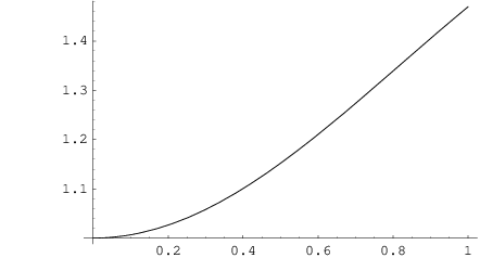
We are in a position to investigate the gravitational behavior of this model in the interior of the star for particular choices of the parameter values in (26). The behaviour of the stellar model is illustrated in terms of graphs of the matter variables and the gravitational potentials. We have generated these graphs with the assistance of the software package Mathematica. For simplicity we make the choices , , and , over the interval , to generate the relevant plots. In Fig. 1 and Fig. 2 we have plotted the metric functions and , respectively. It can easily be seen tha the gravitational potentials remain regular in the interior of the star for . In Fig. 3 we have the behaviour of the energy density , and Fig. 4 gives the representation for the isotropic pressure . We observe that the energy density and the pressure are positive and monotonically decreasing functions in the interior of the star. The electric field intensity is given in Fig. 5 which is positive and monotonically increasing. Thus the quantities , , , and are continuous, regular and well behaved throughout the interior of the star. In Fig. 6 we have plotted on the interval . It can be observed from Fig. 6 that the speed of sound is always less than unity. Consequently the speed of the speed of sound is always less than the speed of light and causality is not violated. Therefore we have demonstrated that there exist particular values for the parameters so that the solution (26) satisfies the requirements for a physically reasonable charged star.
8 Discussion
We have found new solutions (11) to the Einstein-Maxwell system (4), by utilising the coordinate transformation (7), that do not have an uncharged analogue. These solutions are given in terms of elementary functions; other solutions are possible in terms of a general series. Consequently other new exact solutions (22) to the Einstein-Maxwell field equations were found in terms of special functions, namely hypergeometric functions. The electromagnetic field may vanish in the general series solutions and we can regain uncharged solutions. It is possible for hypergeometric functions to be expressed in terms of elementary functions for particular parameter values. We used this feature to find two classes of exact solutions (23) and (24) to the Einstein-Maxwell system in terms of polynomials and product of polynomials and algebraic functions. The simple form of the solutions found facilitate the analysis of the physical features of a charged sphere. For particular parameter values we showed that it is possible to model a physically acceptable charged relativistic sphere.
We should emphasise that the solutions found in the paper depend crucially on the transformation (7) in which and . Consequently we cannot regain the Schwarzchild interior metric or the family of metrics of Hansraj and Maharaj [19] . A different coordinate transformation from (7), allowing for and , must be utilised to regain previously known solutions; a paper outlining this further new class of Einstein-Maxwell solutions is under preparation. Clearly such solutions are possible as the following example illustrates. For the choice of metric function (5), we can show that the system (4) admits the particular exact solution
| (28a) | |||||
| (28b) | |||||
| (28c) | |||||
| (28d) | |||||
| (28e) | |||||
When then and we have uncharged matter with the line element
| (29) |
with equation of state . Thus we have
regained the familiar Einstein universe.
Acknowledgements
We are grateful to the referee for valuable advice. KK thanks the National Research Foundation and the University of KwaZulu-Natal for financial support, and also extends his appreciation to the South Eastern University of Sri Lanka for study leave. SDM acknowledges that this work is based upon research supported by the South African Research Chair Initiative of the Department of Science and Technology and the National Research Foundation.



References
- [1] Ivanov, B.V.: Phys. Rev. D 65, 104001 (2002)
- [2] Komathiraj, K., Maharaj, S.D.: J. Math. Phys., 042501 (2007)
- [3] Sharma, R., Mukherjee, S., Maharaj, S.D.: Gen. Relat. Gravit. 33, 999 (2001)
- [4] Patel, L.K., Koppar, S.K.: Aust. J. Phys. 40, 441 (1987)
- [5] Patel, L.K., Tikekar, R., Sabu, M.C.: Gen. Relat. Gravit. 29, 489 (1997)
- [6] Tikekar, R., Singh, G.P.: Gravitation and Cosmology 4, 294 (1998)
- [7] Gupta, Y.K., Kumar, M.: Gen. Relat. Gravit. 37, 233 (2005)
- [8] Sharma, R., Karmakar, S., Mukherjee, S.: Int. J. Mod. Phys. D 15, 405 (2006)
- [9] Sharma, R., Mukherjee, S.: Mod. Phys. Lett. A 16, 1049 (2001)
- [10] Sharma, R., Mukherjee, S.: Mod. Phys. Lett. A 17, 2535 (2002)
- [11] Thomas, V.O., Ratanpal, B.S., Vinodkumar, P.C.: Int. J. Mod. Phys. D 14, 85 (2005)
- [12] Tikekar, R., Thomas, V.O.: Pramana - J. Phys. 50, 95 (1998)
- [13] Paul, B.C., Tikekar, R.: Gravitation and Cosmology 11, 244 (2005)
- [14] John, A.J., Maharaj, S.D.: Il Nuovo Cimento B 121, 27 (2006)
- [15] Maharaj, S.D., Thirukkanesh, S.: Math. Meth. Appl. Sci. 29, 1943 (2006)
- [16] Thirukkanesh, S., Maharaj, S.D.: Class. Quantum Grav. 23, 2697 (2006)
- [17] Durgapal, M.C., Bannerji, R.: Phys. Rev. D 27, 328 (1983)
- [18] Tikekar, R.: J. Math. Phys. 31, 2454 (1990)
- [19] Hansraj, S., Maharaj, S.D.: Int. J. Mod. Phys. D 15, 1311 (2006)
- [20] Finch, M.R., Skea, J.E.F.: Class. Quantum Grav. 6, 467 (1989)