Loose Hamilton Cycles in HypergraphsThanks: D. Kühn was partially supported by the EPSRC, grant no. EP/D50564X/1. D. Osthus was partially supported by the EPSRC, grant no. EP/E02162X/1. P. Keevash was partially supported by the ERC, grant no. 239696, and by the EPSRC, grant no. EP/G056730/1
Abstract.
We prove that any -uniform hypergraph on vertices with minimum degree at least contains a loose Hamilton cycle. The proof strategy is similar to that used by Kühn and Osthus for the 3-uniform case. Though some additional difficulties arise in the -uniform case, our argument here is considerably simplified by applying the recent hypergraph blow-up lemma of Keevash.
1. Introduction
A fundamental theorem of Dirac [3] states that any graph on vertices with minimum degree at least contains a Hamilton cycle. A natural question is whether this theorem can be extended to hypergraphs.
For this, we first need to extend the notions of minimum degree and of Hamilton cycles to hypergraphs. A -uniform hypergraph or -graph consists of a vertex set and a set of edges each consisting of vertices. We will often identify with its edge set and write if is an edge of . Given a -graph , we say that a set of vertices has neighbourhood . The degree of is . The minimum degree of is the minimum size of such a neighbourhood, that is, .
We say that a -graph is a cycle of order if its vertices can be given a cyclic ordering so that every consecutive pair lies in an edge of and every edge of consists of consecutive vertices. A cycle of order is tight if every set of consecutive vertices forms an edge; it is loose if every pair of adjacent edges intersects in a single vertex, with the possible exception of one pair of edges, which may intersect in more than one vertex. This final condition allows us to consider loose cycles whose order is not a multiple of . Figure 1 shows the structure of each of these cycle types. A Hamilton cycle in a -graph is a sub--graph of which is a cycle containing every vertex of .
Rödl, Ruciński and Szemerédi [11, 12] showed that for any there is an so that if then any -graph on vertices with minimum degree contains a tight Hamilton cycle (this improved an earlier bound by Katona and Kierstead [6]). They gave a construction which shows that this result is best possible up to the error term . In this paper, we prove the analogous result for loose Hamilton cycles.
Theorem 1.1.
For all and any there exists so that if then any -graph on vertices with contains a loose Hamilton cycle.
The case when was proved by Kühn and Osthus [9]. We will use a similar method of proof for general -graphs, but this will be greatly simplified by the use of the recent blow-up lemma of Keevash [7].
Proposition 2.1 shows that Theorem 1.1 is best possible up to the error term . In fact, Proposition 2.1 actually tells us more than this, namely that up to the error term, this minimum degree condition is best possible to ensure the existence of any (not necessarily loose) Hamilton cycle in . This means that the minimum degree needed to find a Hamilton cycle in a -graph of order is .
Whilst finalizing this paper we learnt that Hàn and Schacht [5] independently and simultaneously proved Theorem 1.1, using a different approach. The result in [5] also covers the notion of a -uniform -cycle for (here one requires consecutive edges to intersect in precisely vertices). More recently Kühn, Mycroft and Osthus [10] further developed the method of Hàn and Schacht to include all such that (the remaining values of are covered by the results of Rödl, Ruciński and Szemerédi [11, 12]).
There is also the notion of a Berge-cycle, which consists of a sequence of vertices where each pair of consecutive vertices is contained in a common edge. This is less restrictive than the cycles considered in this paper. Hamiltonian Berge-cycles were studied in [2].

2. Extremal example and outline of the proof
The next proposition shows that Theorem 1.1 is best possible, up to the error term .
Proposition 2.1.
For all integers and , there exists a -graph on vertices such that but does not contain a Hamilton cycle.
Proof. Let and be disjoint sets of size and respectively. Let be the -graph on the vertex set , with an edge if and only if , that is, if contains at least one vertex from . Then has minimum degree . However, any cyclic ordering of the vertices of must contain consecutive vertices from , but then and cannot be contained in a common edge consisting of consecutive vertices, and so cannot contain a Hamilton cycle.
In our proof of Theorem 1.1 we construct the loose Hamilton cycle by finding several paths and joining them into a spanning cycle. Here a -graph is a path if its vertices can be given a linear ordering such that every edge of consists of consecutive vertices, and so that every pair of consecutive vertices of lie in an edge of . Similarly as for cycles, we say that a path is loose if edges of intersect in at most one vertex. The ordering of the vertices of naturally gives an ordering of the edges of . We say that any vertex of which lies in the initial edge of , but not the second edge of , is an initial vertex. Similarly, any vertex of which lies in the final edge of but not the penultimate edge is a final vertex. Also, we refer to vertices of which lie in more than one edge of as link vertices. Thus, for example, a loose path has initial vertices, final vertices, and one link vertex in each pair of consecutive edges.
In Section 3, we shall introduce various ideas we will need in the proof of Theorem 1.1. In particular, we will state a version of the hypergraph regularity lemma due to Rödl and Schacht [13] and Theorem 3.3 due to Keevash [7]. The latter provides a useful way of applying the hypergraph blow-up lemma. In Section 4, we shall prove various auxiliary results, including a result on finding loose paths in complete -partite -graphs, and an approximate minimum degree condition to guarantee a near-perfect packing of with a particular -graph . Finally, in Section 5 we shall prove Theorem 1.1 as follows.
2.1. Imposing structure on .
In Section 5.1 we use the hypergraph regularity lemma to split into -partite -graphs on disjoint vertex sets . These -graphs will be suitable for embedding almost spanning loose paths, and all the vertices of not contained in any of the will be included in an ‘exceptional’ loose path (actually, if is not divisible by , then will contain two consecutive edges which intersect in more than one vertex). The requirement that contains an almost spanning loose path means that the vertex classes of the must have suitable size. We achieve this by first defining a suitable ‘reduced -graph’ of . Then we cover almost all vertices of by copies of a suitable auxiliary -graph . For each copy of , the corresponding sub--graph of is then split into the same number of disjoint .
2.2. The linking strategy.
In Section 5.3 we shall use the structure imposed on to find a Hamilton cycle in by the following process.
- (a)
The -graphs are connected by means of a walk in the ‘supplementary graph’. This graph (which we will define in Section 5.2) has vertices corresponding to the -graphs .
- (b)
Using Lemma 5.2, each edge of is used to create a short ‘connecting’ loose path in joining two different s.
- (c)
and the paths are extended to ‘prepaths’ (these can be thought of as a path minus an initial vertex and a final vertex) and , where and all are sets of size . These prepaths have the property that there are large sets and such that can be extended to a loose path by adding any vertex of as an initial vertex and any vertex of as a final vertex. Similarly there are large sets and so that can be extended to a path by adding any vertex of as an initial vertex and any vertex of as a final vertex. and both lie in the same (for all ).
- (d)
For each and for all those pairs which lie in , we choose a loose path inside from to . For each , we will use the hypergraph blow-up lemma (in the form of Theorem 3.3) to ensure that together all those which lie in use all the remaining vertices of .
- (e)
The loose Hamilton cycle is then the concatenation .
2.3. Controlling divisibility.
Note that the number of vertices of a loose path is modulo . So in order to apply Theorem 3.3 to obtain spanning loose paths in a subgraph of , we need this subgraph to satisfy this condition. So we choose our paths sequentially to satisfy the following congruences modulo .
- (a)
is chosen with .
- (b)
Let be the subset of obtained by removing . (All the will be disjoint from .) Let be the number of times that visits . When choosing , for every it traverses (except the final one) we arrange to intersect in a set of size (the size modulo of the intersection of with the final it traverses is then determined by the sizes of the other intersections). The choice of in (a) ensures that after all have been picked, the remaining part of has size .
- (c)
Each is extended to a prepath by adding and . Similarly, is extended into a prepath by adding and . Now the remaining part of has size .
- (d)
It remains to select paths within each : each uses vertices, so the divisibility conditions are satisfied.
3. Regularity and the Blow-up Lemma
3.1. Graphs and complexes
We begin with some notation. By we denote the set of integers from 1 to . For a set , we use to denote the collection of subsets of of size , and similarly to denote the collection of non-empty subsets of of size at most . We write to mean that . We shall omit floors and ceilings throughout this paper whenever they do not affect the argument.
A hypergraph consists of a vertex set and an edge set, such that each edge of the hypergraph satisfies . So a -graph as defined in Section 1 is a hypergraph in which all the edges are of size . We say that a hypergraph is a -complex if every edge has size at most and forms a simplicial complex, that is, if and then . As for -graphs we identify a hypergraph with the set of its edges. So is the number of edges in , and if and are hypergraphs then is formed by removing from any edge which also lies in . If is a hypergraph with vertex set then for any the restriction of to is defined to have vertex set and all edges of which are contained in as edges. Also, for any hypergraphs and we define to be the hypergraph .
We say that a hypergraph is -partite if its vertex set is divided into pairwise-disjoint parts , in such a way that for any edge , for each . We call the the vertex classes of and say that the partition of is equitable if all the have the same size. We say that a set is -partite if for each . So every edge of an -partite hypergraph is -partite. In the same way we may also speak of -partite -graphs and -partite -complexes. Given a -graph , we define a -complex and and a -complex and . Conversely, for a -complex we define the -graph to be the ‘top level’ of , i.e. . (Here .)
Given a -graph and a set of vertices of , we denote by the sub--graph of obtained by removing all vertices and edges not contained in (in this case, we say is restricted to ). For a -graph and a sub--graph write for .
Let be pairwise-disjoint sets of vertices, and let . Given , we write for the complete -partite -graph whose vertex classes are all the with . The index of an -partite subset of is . Furthermore, given any set , we write . Similarly, given and an -partite -graph or -complex on the vertex set we write for the collection of edges in of index and let . In particular, if is a -complex then is the set of all those vertices in which lie in an edge of (and thus form a (singleton) edge of ). In general, we will often view as an -partite -graph with vertex set . Also, given a -complex we similarly write and . We write for the -graph whose edges are those -partite sets of index for which all proper subsets of belong to . (In other words, a set with index satisfies if and only if for all the edges of which have size and are subsets of form a complete -graph on vertices.) Then the relative density of at index is . The absolute density of is . (Note that .) If is a -partite -complex we may simply write for . Similarly, the density of a -partite -graph on is .
Finally, for any vertex of a hypergraph , we define the vertex degree of to be the number of edges of which contain . Note that this is not the same as the degree defined earlier, which was for sets of vertices. The maximum vertex degree of is then the maximum of taken over all vertices . The vertex neighbourhood of is the set of all vertices for which there is an edge of containing both and . For a -partite -complex on the vertex set we also define the neighbourhood complex of a vertex for some to be the -partite -complex with vertex set and edge set .
3.2. Regular complexes
In this subsection we shall define the concept of regular complexes (which was first introduced in the -uniform case by Rödl and Skokan [15]) in the form used by Rödl and Schacht [13, 14]. This is a generalization of the standard concept of regularity in graphs, where we say that a bipartite graph on vertex classes and forms an -regular pair if for any and with and we have .
In the same way, we say that a -complex is regular if the restriction of to any large subcomplex of lower rank has similar densities to . More precisely, let be an -partite -complex on the vertex set . For any , we say that is -regular if for any with we have
We say is -regular if is -regular for every . Note that if is a graph without isolated vertices, then the definition in the previous paragraph is equivalent to the 2-complex being -regular. To illustrate the definition for , suppose that . Then for instance the top level of is the bipartite subgraph of induced by and and is the set of (graph) triangles in . So roughly speaking, the regularity condition states that if we consider a subgraph of which spans a large number of triangles, then the proportion of these which also form an edge of is close to , i.e. close to the proportion of (graph) triangles in between , and which form an edge of .
Roughly speaking, the hypergraph regularity lemma states that an arbitrary -graph can be split into pieces, each of which forms a regular -complex. The version of the regularity lemma we shall use also involves the notion of a ‘partition complex’, which is a certain partition of the edges of a complete -complex. As before, let be an -partite vertex set. A partition -system on consists of a partition of the edges of for each . We refer to the partition classes of as cells. So every edge of is contained in precisely one cell of . is a partition -complex on if it also has the property that whenever lie in the same cell of , we have that and lie in the same cell of for any . This property of forms an equivalence relation on the edges of , which we refer to as strong equivalence. To illustrate this, again suppose that and . Then if is a partition -complex, , and together yield a vertex partition refining . naturally induces a partition of the complete bipartite graphs induced by the pairs . , and also yield a partition of these complete bipartite graphs. The requirement of strong equivalence now implies that is a refinement of . At the next level, naturally induces a partition of the set of triples induced by and . As before, strong equivalence implies that the partition of these triples is a refinement of .
Let be a partition -complex on . For , the cells of are called clusters (so each cluster is a subset of some ). We say that is vertex-equitable if all clusters have the same size. is -bounded if for every (i.e. if is divided into at most cells by the partition ). Also, for any -partite set , we write for the set of all edges lying in the same cell of as , and write for the -partite -complex whose vertex set is and whose edge set is . (Since is a partition -complex, is indeed a complex.) The partition -complex is -regular if is -regular for every -partite .
Given a partition -complex on and , we can define an equivalence relation on the edges of , namely that are equivalent if and only if and lie in the same cell of for any strict subset . We refer to this as weak equivalence. Note that if the partition complex is -bounded, then is divided into at most classes by weak equivalence. If we let be an -partite -graph on , then we can use weak equivalence to refine the partition of (i.e. two edges of are in the same cell if they are weakly equivalent and similarly for the edges not in ). Together with , this yields a partition -complex which we denote by . If is -regular then we say that is perfectly -regular with respect to . Note that if is -regular then must be -regular too.
Finally, we say that -partite -graphs and on are -close if for every , that is, if there are few edges contained in but not in and vice versa.
We can now present the version of the regularity lemma we shall use to split our -graph into regular -complexes. It actually states that there is some -graph which is close to and which is regular with respect to some partition complex. This will be sufficient for our purposes, as we shall avoid the use of any edges in , so every edge used will lie in both and . There are various other forms of the regularity lemma for -graphs which give information on itself (the first of these were proved in [15, 4]) but these do not have the hierarchy of densities necessary for the application of the blow-up lemma (see [7] for a fuller discussion of this point). The version below is due to Rödl and Schacht [13] (actually it is a very slight restatement of their result).
Theorem 3.1 (Theorem 14, [13]).
Suppose integers and reals satisfy and where divides . Suppose also that is an -partite -graph whose vertex classes form an equitable partition of its vertex set , where . Then there is an -bounded -regular vertex-equitable partition -complex on and an -partite -graph on that is -close to and perfectly -regular with respect to .
Here (and later on) we write to mean that we can choose the constants from right to left. More precisely, there are increasing functions such that, given , whenever we choose some , and , all calculations needed in the proof of the subsequent statement are valid. Hierarchies with more constants are defined similarly.
One important property of regular complexes is that they remain regular when restricted to a large subset of their vertex set. For regular -partite -complexes this property is formalised by the following lemma, a special case of Lemma 6.18 in [7].
Lemma 3.2 (Restriction of regular complexes).
Suppose , and that is an -regular -partite -complex on the vertex set such that for each and . Let be a subset of such that for each . Then the restriction of to is -regular, with and .
3.3. Robustly universal complexes.
Apart from Theorem 3.1, the other main tool we shall use in the proof of Theorem 1.1 is the recent hypergraph blow-up lemma of Keevash. This result involves not only a -complex , but also a -graph of ‘marked’ edges on the same vertex set. If the pair is ‘super-regular’, then this blow-up lemma can be applied to embed any spanning bounded-degree -complex in , that is, within but avoiding any marked edges. We will apply this with where is the -graph given by Theorem 3.1. Super-regularity is a stronger notion than regularity. A result in [7] states that every -regular -complex can be made super-regular by deleting a few of its vertices. Unfortunately, the notion of hypergraph super-regularity is very technical, but the following definition from [7] avoids many of these technicalities. Let be a -partite -complex. Roughly speaking, we say that is robustly -universal if the following holds: even after the deletion of many vertices of , the resulting complex has the property that one can find in a copy of any -partite -complex which has vertex degree at most and whose vertex classes are the same as those of . Condition (i) puts a natural restriction on the number of vertices we are allowed to delete from the neighbourhood complex of a vertex of and condition (iii) states that for a few vertices of we can even prescribe a ‘target set’ in into which will be embedded.
Definition. (Robustly universal complexes) Suppose that is a -partite -complex on with for each . We say that is -robustly -universal if whenever
- (i)
are sets with for all , such that writing and we have for any and ,
- (ii)
is a -partite -complex of maximum vertex degree at most on some vertex set with for all ,
- (iii)
satisfies for every , and sets satisfy for each , where for each we let be such that ,
then contains a copy of , in which for each the vertices of correspond to the vertices of , and corresponds to a vertex of for every .
So our use of the blow-up lemma will be hidden through this definition. Of course, we shall also need to obtain robustly universal complexes. This is the purpose of the next theorem, which states that given a regular -partite -complex with sufficient density, and a -partite -graph on the same vertex set which is small relative to , we can delete a small number of vertices from their common vertex set so that is robustly universal. It is a special case of Theorem 6.32 in [7].
Theorem 3.3.
Suppose that , is a -partite -complex on with for every , is -regular with and , and with . Then we can delete at most vertices from each to obtain , and such that
- (i)
and for every , and
- (ii)
is -robustly -universal.
4. Preliminary results
In this section we will collect the preliminary results we need to prove Theorem 1.1. In order to apply Theorem 3.3, we need to know under what conditions we can find particular loose paths in complete -partite -graphs, which is the topic of the next subsection.
4.1. Loose paths in complete graphs
The problem of when we can find particular loose paths in a complete -partite -graph can be reformulated in terms of the question of which strings satisfying certain adjacency conditions can be produced from a fixed character set; the following lemma is the result we will need.
Lemma 4.1.
Let and be integers such that for all , and . Then for any there exists a string of length on alphabet such that the following properties hold:
- (1)
no two consecutive characters are equal,
- (2)
the first character is not and the final character is not ,
- (3)
the number of occurrences of character is .
Proof. Note that the conditions on and the imply that . We will construct the required string by starting with an ‘empty string’ of blank positions, and for each inserting precisely copies of character . This ensures that condition (3) will be satisfied. We shall fill the empty positions in the following order: first the first position, then the third, and so on through the odd-numbered positions, until we reach either position or position (dependent on whether is odd or even). We then fill the second position, then the fourth, and so on until all positions are filled. Note that if we proceed by inserting all copies of one character, then all the copies of another character, and so forth, then condition (1) must be satisfied. This is because to get two consecutive copies of , we must have inserted a copy of at some odd position , then , , and so on until reaching or , and then filled even positions . However, this would imply that we had inserted at least copies of character , contradicting the fact that .
We therefore only need to determine an order to insert the different characters so as to satisfy (2). We first consider the case , say and . In this case we insert first, last, and the remaining character blocks in any order in between. Clearly this prevents the first character from being and the last from being , and so (2) is satisfied. Now we may assume , say . Then if is odd, we insert the characters in the following order: . Then all the copies of must be in even positions (since ), and so (2) is satisfied. Alternatively, if is even, we insert first for some with , then , and then the remaining blocks of characters in any order. (Note that these include at least one character other than and since and imply that at least three have .) So neither the first nor last character can be , and so (2) is again satisfied.
The next lemma is the result we were aiming for in this section, giving information about which loose paths can be found in complete -partite -graphs. Note that the maximum vertex degree of a loose path is two, and so this lemma will tell us when we can find a loose path in a robustly universal -complex.
Lemma 4.2.
Let be a complete -partite -graph on the vertex set . Let be integers with for each . Suppose that
- •
is an integer, and
- •
for all .
Then for any , there exists a loose path in with an initial vertex in , a final vertex in , and containing vertices from for each .
Proof. Note first that is the number of edges such a path must contain. Let for each , so that . By Lemma 4.1 we can find a string of length on the alphabet such that appears times, no two consecutive characters are identical, the first character is not and the final character is not . Let be the th character of . To construct a loose path in , first choose any vertex from to be the initial vertex of , and any vertex from to be the final vertex of . We also use to choose the link vertices of : choose the th link vertex (i.e. the vertex lying in the intersection of the th and th edges of ) to be any member of not yet chosen. We have now assigned two vertices to each edge of . Finally, we complete by assigning to each edge one as yet unchosen vertex from each of the classes not yet represented in that edge. This is possible since precisely link vertices are from the class and so the total number of vertices used from is . Since is complete we know that each edge of is an edge of , and so is a loose path satisfying all the conditions of the lemma.
4.2. Walks and connectedness in -graphs
A walk in a hypergraph consists of a sequence of edges of and a sequence of (not necessarily distinct) vertices of , satisfying for all , and also , and for all . The length of is the number of its edges. We say that is the initial vertex of , is the final vertex of , and that are the link vertices of . By a walk from to we mean a walk with initial vertex and final vertex .
Note that the vertices of a hypergraph can be partitioned using the equivalence relation , where if and only if either or there exists a walk from to . We call the equivalence classes of this relation components of . We say that is connected if it has precisely one component. Observe that all vertices of an edge of must lie in the same component. Finally, note that if is a connected hypergraph of order , then for any two vertices of we can find in a walk from to of length at most in .
4.3. Random splitting
In this section we shall obtain, with high probability, a lower bound on the density of a subgraph of a -partite -graph chosen uniformly at random. We will use Azuma’s inequality on the deviation of a martingale from its mean.
Lemma 4.3 (Azuma [1]).
Suppose is a martingale, i.e. a sequence of random variables satisfying , and that for some constants and all . Then for any ,
Lemma 4.4.
Suppose , and that is a -partite -graph on the vertex set , where for each . Suppose also that has density and that for each we have . If we choose a subset with uniformly at random and independently for each , and let , then the probability that has density is at least . Moreover, the same holds if we choose by including each vertex of independently with probability .
Proof. Let . To prove the first assertion, we obtain our subsets through the following two-stage random process, independently for each . First we assign the vertices of each into sets and independently at random, with each vertex being assigned to with probability , and assigned to otherwise. Then, in the (highly probable) event that we have we shall select uniformly at random a set of vertices to transfer between and to obtain from the set with . For each , no subset of size is more likely to result from this process than any other, so we have chosen each uniformly at random. It remains to show that is likely to have high density. We do this by noting that is likely to have high density (where ) and that with high probability we will only need to transfer a small number of vertices to form , which can have only a limited effect on the density.
More precisely, let be an ordering of the vertices of , and for each let the random variable take the value 1 if , and 0 otherwise. Recall that we write to denote the number of edges of a -graph . For all we now define random variables by . Then the sequence is a martingale, , and as we formed each by assigning vertices of independently at random into and , we have . Also, for any vertex , let be such that (i.e. is the index of ). Then for all . Thus we can apply Lemma 4.3 to obtain
Therefore the event that has probability at least . Also, by a standard Chernoff bound, for each the event that has probability at least . Thus with probability at least all of these events will happen. Now, if , we choose a set of vertices of uniformly at random and move these vertices from to . Similarly, if , then we choose a set of vertices of uniformly at random and move these vertices to . In either case, for any this action can decrease by at most . Thus if we let be the set obtained from in this way, we have , proving the first part of the lemma.
The proof of the ‘moreover part’ is the same except that we can omit the ‘transfer’ step at the end of the proof.
4.4. Decomposition of into copies of
Let denote the -graph whose vertex set is the union of disjoint sets of size and whose edges consist of all -tuples of the form , with and (see Figure 2).

So . An -packing in a -graph is a collection of pairwise vertex-disjoint copies of in .
Lemma 4.5.
Suppose , and that is a -graph on such that for all but at most sets . Then has an -packing which covers more than vertices of .
Proof. Let be an -packing of of maximum size, so . Let be the set of uncovered vertices, and suppose that . Let . Our first aim is to choose disjoint sets in so that and for all . Note that implies that . So we can greedily choose disjoint such that for all . Let . We claim that . Otherwise, consider the bipartite graph with vertex classes and , where we join to if is an edge of . Note that cannot contain a complete bipartite graph with vertices in and vertices in , as this would correspond to a copy of contained in , which is impossible as is a maximum size -packing. However, by definition of we have for every , and double-counting pairs with and gives
a contradiction. This proves the claim, and by relabelling the we can assume that and for all .
Now we show how to enlarge the -packing . For let
Since for each we have
and so . We now double-count pairs with and . The number of such pairs is
So we can find some and with such that for every . For each and each fix some -set (which is possible by definition of ). Then we can choose with so that for all and every . For each we write for with .
We will now use the to find new copies of that only intersect of the copies in our packing. We arbitrarily divide into sets of size and label for all . The new copies of are obtained for each by identifying with and with . Replacing the copies by we obtain a larger -packing. This contradiction completes the proof.
Corollary 4.6.
Lemma 4.5 still holds if we insist that the sub--graph of induced by the vertices covered by the -packing must be connected.
Proof. Apply Lemma 4.5 to obtain an -packing in with , and let be the sub--graph of induced by . By hypothesis at most sets have fewer than neighbours in and so at most sets have no neighbours in . By the definition of a component, no edges of contain vertices from different components of . Therefore the largest component of must contain at least vertices. Indeed, if not then there are at least sets which meet at least two components of and thus have no neighbours in , a contradiction (we can obtain such a set by choosing vertices arbitrarily in and then choosing the final vertex in a different component of than the first vertex). Thus we may take the -packing consisting of all those copies of with .
5. Proof of Theorem 1.1
In our proof we will use constants that satisfy the hierarchy
Furthermore, for any of these constants , we use and assume that the above hierarchy also extends to the additional constants, e.g. .
5.1. Imposing structure on
5.1.1. Step 1. Applying the regularity lemma
Let be the sub--graph obtained from by removing up to vertices so that is divisible by . Let be an equitable -partition of the vertices of , and let consist of all those edges of that are -partite sets in . Then is an -partite -graph with order divisible by , and so we may apply the regularity lemma (Theorem 3.1), which yields an -bounded -regular vertex-equitable partition -complex on and an -partite -graph on that is -close to and perfectly -regular with respect to .
Let . So any edge of is also an edge of . Let be the clusters of . So and is -partite with vertex classes . Note that since is -bounded. Moreover, since is vertex-equitable, each has the same size. So let .
As is usual in regularity arguments, we shall consider a reduced -graph, whose vertices correspond to the clusters , and whose edges indicate that within the cells of corresponding to the edge we can find a subcomplex to which we can apply Theorem 3.3. For this we would like to have high density in these cells, and to have low density. Thus we define the reduced -graph on as follows: a -tuple of vertices of corresponds to the -partite union of clusters. The edges of are precisely those for which has density at least (i.e. ) and for which has density at most (i.e. ).
Now, the edges in the reduced graph are useful in the following way. Given an edge , let again. Using weak equivalence (defined in Section 3.2), the cells of induce a partition of the edges of . Recall that . Therefore at most edges of can lie in sets with . Furthermore, (as ) and so at most edges of can lie in sets with . Together with the fact that this now implies that more than edges of lie in sets with and . Thus there must exist such a set that also satisfies . Fix such a choice of and denote it by . Let be the -partite -complex on the vertex set consisting of and the cells of that ‘underlie’ , i.e. for any edge we have
| (1) |
(Recall that was defined in Section 3.2.) We also define the -partite -graph on the vertex set . Then the following properties hold:
- (A1)
is -regular.
- (A2)
has -th level relative density .
- (A3)
has absolute density .
- (A4)
satisfies .
- (A5)
for any .
Indeed, (A1) follows from (1) since is perfectly -regular with respect to . To see (A2), note that and so by our choice of . Similarly, (A3) follows from our choice of since
(A4) holds since and . Finally, (A5) follows from (1) and the fact that for all .
5.1.2. Step 2. Choosing an -packing of
The next step in our proof is to use Corollary 4.6 to find an -packing in the reduced -graph . For this we shall need an approximate minimum degree condition for . Let
We shall show that is small, that is, that almost all -tuples of vertices of have degree at least in . Consider how many edges of do not belong to for some edge . (Recall that .) There are three possible reasons why an edge does not belong to such a restriction:
- (i)
is not an edge of . This could be because lies in but not , in but not , or in but not . There are at most edges of the first type, at most of the second type, and at most of the third type.
- (ii)
contains vertices from such that the restriction of to satisfies , where . (Note that since and thus is -partite, are all distinct.) Since and are -close and thus there are at most edges of this type.
- (iii)
contains vertices from such that the restriction of to has density less than . There are at most edges of this type.
Therefore there are fewer than edges of that do not belong to the restriction of to for some , and so we have
Since we deduce that , and so (since ). This allows us to apply Corollary 4.6 (with ) to obtain an -packing in with , such that the sub--graph of induced by is connected. For each , let the vertex set of be , with each of size , so that the edge set is .
5.1.3. Step 3. Forming the exceptional path.
Given a sub--graph of and a cluster , we say that belongs to if . Let contain the at most vertices of we removed at the start of the proof, and also the vertices in all those clusters not belonging to some copy of in our packing (there are at most of the latter). We will incorporate these vertices into a path which will later form part of our loose Hamilton cycle. We also include in an arbitrary choice of vertices from each for which for some and some (we do not modify any of the for which ). We add up to more vertices from (say) to so that . We delete all these vertices from the clusters they belonged to and still write for the subcluster of a cluster obtained in this way. This gives .
Now, we shall construct a path in , which will contain all the vertices in and avoid all the clusters with . Let . So we shall use only vertices from and in forming . Recall that if is not a multiple of , then a loose Hamilton cycle contains a single pair of edges which intersect in more than one vertex: we shall make allowance for this here. Choose satisfying , and . Now choose distinct such that and (we shall see in a moment that such exist). These edges will be the first 2 edges of . To complete , let be any partition of the vertices of into sets of size . We proceed greedily in forming : for each choose any such that (where the are all chosen to be distinct).
Let us now check that there will always be such a vertex available. Indeed, every set in has at least neighbours and we can choose any such neighbour which lies in and has not already been used. But and at most vertices have been used before. Thus (since ) for each choice of an we have at least vertices of to choose from. Moreover, these vertices must be contained in at least different such that (). Thus we can avoid choosing a vertex from any single more than times. The path thus formed has edges , and for all . So all the vertices of are included in . For each cluster , we still denote the subset of lying in by . Then each with for some still satisfies , and each with for some satisfies
| (2) |
In addition
| (3) |
Note that need not be a loose path, but that even if it is not it may still form part of a loose Hamilton cycle. Also observe that .
5.1.4. Step 4. Splitting our copies of .
The next step of the proof will be to split the copies of (more precisely the clusters belonging to the ) into sub--complexes of that we shall later use to embed spanning loose paths. Consider any . For convenient notation we identify each in with (but recall that they are disjoint sets). For each we have , and so we can partition uniformly at random into pairwise disjoint subsets , each of size . Similarly, given with , (2) and the fact that imply that we can partition uniformly at random into pairwise disjoint subsets and so that and for all . Figure 3 shows how we do this in the case .
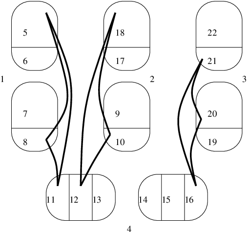
We arrange these pieces into collections of sets as follows: for each and each we have a collection consisting of , and . ( of these collections are illustrated in Figure 3.) For convenient notation we relabel these collections as with , where for all we have
| (4) |
and
| (5) |
((5) follows from (2) using the fact that all the have equal size.) Let , so each is a -partite set, on which we shall now find a sub--complex of that is suitable for applying Theorem 3.3.
Consider any copy in our -packing. Note that for each of the collections obtained by splitting up the clusters belonging to there is an edge such that each lies in a cluster belonging to (and these clusters are distinct for each of ). Recall that denotes the union of all the clusters belonging to . Let denote the restriction of the -partite -complex (which was defined in Section 5.1.1) to , i.e. . Let . We claim that we may choose the above collections such that
| (6) |
Indeed, since , has absolute density at least and has density at most . Since and this shows that has density at least . Lemma 4.4 now implies that each has density at least with probability , and so with non-zero probability this is true for all .
Lemma 3.2 and properties (A1)–(A3) and (A5) imply that is an -regular -partite -complex on the vertex set , with absolute density , relative density , and for each . Moreover, using , property (A4) and the fact that we see that
So by Theorem 3.3 we can delete at most vertices from each so that if we let consist of the undeleted vertices, and let , and , then is -robustly -universal, and for every . In particular, the latter two conditions together imply that for every . Let denote the set of vertices deleted from any , so . By deleting up to more vertices if necessary, we may assume that is divisible by . The latter will help us to extend into a path which contains all the vertices in .
5.1.5. Step 5. Extending the exceptional path .
When extending in order to incorporate , we shall have to remove some more vertices from some of the , and we wish to do this so that the remainder satisfies (i) in the definition of robust universality. For this reason, we partition each into two parts and as follows (where we write for ):
- (B1)
For all and every we have .
- (B2)
Every set of vertices of has at least neighbours in .
(Recall that for a -complex , denotes the ‘th level’ of .) To see that such a partition exists, consider a partition obtained by assigning each vertex to a part with probability independently of all other vertices. (B2) is then satisfied with high probability by a standard Chernoff bound. Now consider (B1). The ‘moreover’ part of Lemma 4.4 implies that with high probability we have for all and for all that . Also, a standard Chernoff bound implies that with high probability for all . Thus
Now, we shall extend our path to include the vertices in , using only vertices from . We proceed similarly to when constructing . So we split into sets of size (so ). Letting be a final vertex of , for , we successively choose to be a neighbour of the -tuple contained in some and not already included in , and extend by the edge , continuing to denote the extended path by . Recall that originally contained at most vertices. Since , after each extension of we shall have . So (B2) implies that for each choice of we have at least suitable vertices and hence at least of the sets contain such a suitable vertex. This shows that we can choose the in such a way that at most vertices are chosen from any single .
For each let be the vertices remaining after the removal from of the at most vertices used in extending , let , and let . By (6) there are at least vertices such that lies in some for which at least edges of contain . So we may add two further edges of to (one at each end) so that the new path has an initial vertex and a final vertex which each lie in at least edges of their respective . (We also delete the vertices of these additional two edges from their , and ). Note that may be contained in some (and the same is true of ), but by (B2) we may choose these two additional edges so that all other vertices used lie in some .
We claim that the above steps give us the following useful structure: a path which is ready to form part of a loose Hamilton cycle, and disjoint -partite vertex sets supporting -complexes and -graphs for each which satisfy the following properties.
- (C1)
Every vertex of lies in either the path or precisely one of the -partite sets .
- (C2)
For each , is a -partite sub--complex of on the vertex set . is the -partite -graph , and . Clearly these statements remain true after the deletion of up to vertices of .
- (C3)
Even after the deletion of up to vertices of , the following statement holds. Let be a -partite -complex on the vertex set , where for each , and let have maximum vertex degree at most . Let and suppose we have and sets with for each (where is such that ). Then contains a copy of , in which for each the vertices of correspond to the vertices of , and each corresponds to a vertex in .
- (C4)
For each , has density at least , even after the deletion of up to vertices of .
- (C5)
If we delete up to vertices from any , and let for each after these deletions, and let , then for all .
- (C6)
The initial vertex of lies in at least edges of , where is such that . The analogue holds for the final vertex of .
(When we talk of removing a vertex of we implicitly mean that , and are all restricted to the remaining vertices of .) These properties hold for the following reasons. (C1) holds as every vertex deleted from an has been added to , whilst (C2) is clear as whenever we deleted vertices we simply restricted and to the remaining vertices. For (C3), recall that was -robustly -universal. Moreover, for all and all we have , since we ensured that we only deleted vertices from any single (and at most two from ). Furthermore by (B1) we know that for any . (Also, even if we had arbitrarily deleted a further vertices from when obtaining , and , these bounds would still hold.) So satisfies (i) in the definition of a robustly universal complex (where plays the role of ). The sets satisfy (iii) in the definition and so we can find the required copy of (even after the deletion of up to more vertices of ). (C4) follows from (6) and the fact that was formed by deleting at most vertices from . Similarly, for (C5) note that (even after up to more deletions) we have deleted at most vertices from each since we split the clusters to form the . So by (4), after these deletions we must have
- •
,
- •
, and
- •
for ,
and by (5) we must have
- •
Since , we deduce that
- •
, and
- •
So property (C5) follows. Finally, (C6) follows from the final step in the construction of , in which we added an extra edge to each end of so that (C6) would be satisfied.
5.2. The supplementary graph
Roughly speaking, our aim is to find a spanning loose path in each (and thus in ) such that all these paths together with form a loose Hamilton cycle in . So we have to ensure that the complete -partite -graph on contains a spanning loose path (for this, we will need ) and we need to join up all the loose paths we find in the . The purpose of this section is to find the ‘connecting loose paths’ which join up the in such a way that the divisibility problems are dealt with as well. To do this, we first define a supplementary hypergraph whose vertices correspond to the . We will show that is connected and that ‘along’ edges of we can find our loose paths in which join up all the .
The vertex set of the supplementary hypergraph is . A subset of size at least 2 is an edge of if there exists an edge such that for all there are and with and . (We fix one such edge for every .) Then every edge of has size at most . We say that belongs to an edge if . Similarly, belongs to some subhypergraph if .
Lemma 5.1.
The supplementary graph is connected.
Proof. Recall that we chose the copies of in such a way that the sub--graph of induced by is connected. Suppose that is not connected. Let be a component of and let . Let for some . So corresponds to the set of all those clusters which meet some belonging to . Define similarly. Then and thus contains some edge intersecting both and . But then corresponds to an edge of intersecting both and , a contradiction.
The next lemma shows that within the belonging to an edge of , we can find a reasonably short loose path in and we may choose (modulo ) how many vertices this path uses from each . Using the connectedness of , this will allow us to find the connecting loose paths which join up the whilst having control over the divisibility properties. We shall also insist that the path in Lemma 5.2 avoids a number of ‘forbidden vertices’, to enable us to ensure that our connecting loose paths are disjoint, and that the endvertices of these paths lie in many edges of the relevant .
Lemma 5.2.
Suppose that and that for every there is an integer such that and . Let be distinct. Moreover, suppose that is a set of at most ‘forbidden’ vertices of . Then in the sub--graph of induced by we can find a loose path with the following properties.
- •
contains at most vertices.
- •
has an initial vertex in and a final vertex in .
- •
for each .
- •
contains no forbidden vertices, i.e. .
- •
lies in at least edges of , and lies in at least edges of .
Proof. Recall that in Section 5.1.1 we assigned a -partite -complex to every edge such that (A1)–(A5) are satisfied. To simplify notation, we write for the edge corresponding to and suppose that . For each choose and such that and such that . To simplify notation we write for , and assume that and . For each let be the set of all with . So the sets are disjoint and their union is . Pick some and let and for all . Our path will consist of vertices from each (modulo ) and thus of vertices from each (modulo ).
Since satisfies (A1)–(A3) and (A5), Lemma 3.2 implies that the restriction is -regular, with absolute density at least , relative density at index at least and . Furthermore, (A4) together with the fact that imply that
Thus Theorem 3.3 implies that we can delete vertices from each to obtain subsets such that is -robustly -universal, where .
Now, let . Then and so is an integer. Furthermore, , and so for each . Thus by Lemma 4.2 we can find a loose path in the complete -partite -graph on the vertex set , beginning in , finishing in and using vertices from each . Since is -robustly -universal, we can find such a loose path in and hence in . (Indeed, we can do this by finding the complex , which has maximum vertex degree at most . Note that we use the definition with in (i)). Note that contains at most vertices.
To see that we can insist on the final condition of the lemma, recall that by (C4). Thus for all at least vertices of lie in at least edges of , and so we may restrict the initial and final vertices of to these sets of vertices (minus the vertices of ) by (iii) in the definition of robust universality.
5.3. Constructing the loose Hamilton cycle
As discussed before, our Hamilton cycle in will consist of and paths in each as well as paths connecting the . However, we need to make sure that all these paths join up nicely, motivating the following definition. Suppose is a path in some -graph with initial vertex and final vertex . Also, let be disjoint sets of size . Then is a prepath. Note that is not (the vertex set of) a -graph, but that if we can find vertices such that , then adding and to gives another path. We refer to all such vertices as possible initial vertices of and to all such vertices as possible final vertices. If , and are disjoint loose paths, are as before, is also the final vertex of and is also the initial vertex of then and together with form a single loose path, illustrating how we shall join paths together.
We start by converting our exceptional path into a prepath. Recall that and that the initial vertex of and its final vertex satisfy (C6). Let and be such that . Pick any with . (C4) and (C6) together imply that there is a set for which contains at least vertices which form an edge of together with . Let be such a set of vertices. Similarly, letting , be such that , there is a set for which contains at least vertices which form an edge of together with . Let be such a set of vertices. Let be the prepath . Then is a set of possible initial vertices of and is a set of possible final vertices. (We do not remove from and from at this stage.)
Since by Lemma 5.1 the supplementary graph is connected, we can find a walk from to in such that every appears as an initial, link or final vertex in (these vertices were defined in Section 4.2) and such that has length . Let be the edges of this walk, let , and let be the link vertices of the walk. For each , let , that is, the number of times appears as an initial, link or final vertex in . So for every and .
Our next aim is to apply Lemma 5.2 to each edge in order to find a loose path in , which we will extend to a prepath with many possible initial vertices in and many possible final vertices in . We shall do this for each in turn. So suppose that and that for all we have defined loose paths in as well as sets extending to a prepath which satisfy the following properties:
- (D1)
lies in the sub--graph of induced by and contains at most vertices.
- (D2)
The initial vertex of lies in and its final vertex lies in .
- (D3)
and .
- (D4)
There is a set of at least possible initial vertices for . Similarly, there is a set of at least possible final vertices for .
- (D5)
All the prepaths are disjoint.
- (D6)
For each and all let , where . For each set . Then for every with we have . Moreover .
Let us now show how to find , and . Apply Lemma 5.2 with , , and with to find a loose path which satisfies (D1), (D2), (D6) and is disjoint from . Moreover, the initial vertex of lies in at least edges of , and the final vertex of lies in at least edges of . We can now use the latter property to choose sets and which extend to a prepath satisfying (D3)–(D5). The argument for this is similar to that for the extension of to . Altogether this shows that we can find prepaths satisfying (D1)–(D6).
For each we let be the maximal integer such that . Thus by (D1). But if then (D5) and (D6) together imply that
and so . We claim that this also holds if . To see this, recall that since is loose, we have for each . Hence
as . Let . Since by (D3) for each there are exactly vertices of which lie in but not in , this in turn implies that
| (7) |
Let , , , and . In order to complete our prepaths to a Hamilton cycle we wish to choose disjoint loose paths within each which together contain all the vertices in and which ‘connect’ successive prepaths . We achieve this as follows. Let be the set of all with . So is the set of positions at which occurs as an initial, final or link vertex in our walk and . Let be the elements of . Then we choose the () in such a way that the initial vertex of lies in and its final vertex lies in , all the are disjoint and together they cover all the vertices in . To see that this can be done, first note that . So using Lemma 4.2 together with (C5) and (7) it is easy to check that the complete -partite -graph on contains such paths (e.g. first choose , each consisting of precisely 2 edges, and then apply (C5) and Lemma 4.2 to find a loose path containing all the remaining vertices of ). Now (C3) and (D4) together imply that contains the -complexes induced by these paths (i.e. it contains ). But this means that we can find the required paths in each .
Finally, for each write for and for its initial and for its final vertex (where is as defined in the previous paragraph). To obtain our Hamilton cycle in we first traverse , then we use the edge in order to move to the initial vertex of . (This is possible since .) Now we traverse and use the edge to get to . (Again, this is possible since .) Next we traverse and use the edge to move to . We continue in this way until we have reached the initial vertex of again. (So in the last step we traversed and used the edge .) This completes the proof of Theorem 1.1.
References
- [1] K. Azuma, Weighted sums of certain dependant random variables, Tôhoku Math. J. 19 (1967), 357–367.
- [2] J.C. Bermond, A. Germa, M.C. Heydemann and D. Sotteau, Hypergraphes hamiltoniens, Prob. Comb. Théorie graph Orsay 260 (1976), 39–43.
- [3] G.A. Dirac, Some theorems on abstract graphs, Proc. London. Math. Soc. 2 (1952), 69–81.
- [4] W.T. Gowers, Hypergraph Regularity and the multidimensional Szemerédi Theorem, Annals of Math. 166 (2007), 897–946.
- [5] H. Hàn and M. Schacht, Dirac-type results for loose Hamilton cycles in uniform hypergraphs, J. Combinatorial Theory B 100 (2010), 332–346.
- [6] G.Y. Katona and H.A. Kierstead, Hamiltonian chains in hypergraphs, J. Graph Theory 30 (1999), 205–212.
- [7] P. Keevash, A hypergraph blow-up lemma, Random Structures and Algorithms, to appear.
- [8] Y. Kohayakawa, V. Rödl and J. Skokan, Hypergraphs, quasi-randomness, and conditions for regularity, J. Combinatorial Theory A 97 (2002), 307–352.
- [9] D. Kühn and D. Osthus, Loose Hamilton cycles in 3-uniform hypergraphs of high minimum degree, J. Combinatorial Theory B 96 (2006), 767–821.
- [10] D. Kühn, R. Mycroft and D. Osthus, Hamilton -cycles in uniform hypergraphs, J. Combinatorial Theory A 117 (2010), 910–927.
- [11] V. Rödl, A. Ruciński and E. Szemerédi, A Dirac-type theorem for 3-uniform hypergraphs, Combin. Probab. Comput. 15 (2006), 229–251.
- [12] V. Rödl, A. Ruciński and E. Szemerédi, An approximate Dirac-type theorem for -uniform hypergraphs, Combinatorica 28 (2008), 229–260.
- [13] V. Rödl and M. Schacht, Regular partitions of hypergraphs: regularity lemmas, Combin. Probab. Comput. 16 (2007), 833–885.
- [14] V. Rödl and M. Schacht, Regular partitions of hypergraphs: counting lemmas, Combin. Probab. Comput. 16 (2007), 887–901.
- [15] V. Rödl and J. Skokan, Regularity lemma for uniform hypergraphs, Random Structures & Algorithms 25 (2004), 1–42.
Peter Keevash, Richard Mycroft, School of Mathematical Sciences, Queen Mary, University of London, Mile End Road, London, E1 4NS, United Kingdom, {p.keevash,r.mycroft}@qmul.ac.uk
Daniela Kühn, Deryk Osthus, School of Mathematics, University of Birmingham, Birmingham, B15 2TT, United Kingdom, {kuehn,osthus}@maths.bham.ac.uk