William I. Fine Theoretical Physics Institute
University of Minnesota
FTPI-MINN-08/31
UMN-TH-2713/08
August 2008
The spontaneous breaking of a metastable string
A. Monin
School of Physics and Astronomy, University of Minnesota,
Minneapolis, MN 55455, USA,
and
M.B. Voloshin
William I. Fine Theoretical Physics Institute, University of
Minnesota,
Minneapolis, MN 55455, USA
and
Institute of Theoretical and Experimental Physics, Moscow, 117218, Russia
We consider the phase transition of a string with tension to a string with a smaller tension . The transition proceeds through quantum tunneling, and we calculate in arbitrary number of dimensions the pre-exponential factor multiplying the leading semiclassical exponential expression for the rate of the process. At the found formula for the decay rate also describes a break up of a metastable string into two pieces.
1 Introduction
String-like configurations arise in a great number of actual systems, such as superconductors and polymers, in theoretical models of non-Abelian dynamics, such as models of QCD confinement, and as topological defects in models with spontaneous breaking of gauge or global symmetries. In some of these situations the string configurations are not absolutely stable, but are rather metastable with respect to either a complete breaking, or a break up with a string of lower tension emerging instead of the initial string. The former situation is relevant e.g. for a break up of a QCD string with formation of a quark - antiquark pair, or a formation of a monopole - antimonopole pair[1], and also in a whole class of theories with spontaneous symmetry breaking[2]. The latter situation involving a phase transition between states of a string with different tension is found e.g. in Abelian Higgs models embedded in non-Abelian theories[3]. It is clear that the latter case is more general, since the breaking of a string into ‘nothing’ can be considered as a transition into a string with zero tension.
The transition of a metastable string with the tension to a string with a lower tension is quite analogous to decay of metastable vacuum[4, 5], or the Schwinger process of creation of pairs of charged particles by electric field[6]. Indeed, if a piece of length is converted into the lower phase, the gain in the energy is . The barrier that inhibits the process is created by the energy associated with the interface between the phases of the string, e.g. the mass of the monopole in the examples of Ref.[1] or [3]. The transition involves two such interfaces, so that the ‘length’ energy gain exceeds the barrier energy only starting from a critical size of the ‘true’ phase . Once a critical piece has nucleated due to tunneling, the additional energy gain is spent on acceleration of the ends of this piece in its expansion, which eventually converts the whole length of the initial string. Thus the probability of the transition is given by the rate of nucleation of the critical gaps in the initial string. This rate per unit time and per unit length of the metastable string is given by the semiclassical expression[1, 2, 3]
| (1) |
where , the pre-exponential factor, is the main subject of the calculation in this paper. The semiclassical expression is formally applicable as long as the exponential power, determined by the action on the tunneling trajectory is large, which requires
| (2) |
The pre-exponential factor is found from a calculation of the path integral over small deviations from the semiclassical tunneling trajectory[7]. The result of such calculation in a (1+1) dimensional theory, can be readily copied from the corresponding expressions in equivalent (1+1) dimensional problems: either that of pair creation in electric field[6], or of false vacuum decay[8, 9, 10],
| (3) |
However, the equivalence of the string transition to already solved problems does not hold for string in more than two dimensions. The loss of the relation to the false vacuum decay is due to the obvious difference in the dimensionality of the relevant objects, while the loss of equivalence to the Schwinger process is due to a different dependence of the action on the deviations of the tunneling trajectory in the transverse directions. Indeed small deviations of the particles in the Schwinger process perpendicular to the external electric field involve only the particles themselves, while a transverse displacement of an end of a string involves both the ‘particle’ (of the mass ) and an adjacent part of the string. In this paper we calculate the relevant path integral and find the pre-exponential coefficient for arbitrary number of space-time dimensions . Our final result for the transition rate reads as
| (4) |
with being the renormalized value of the mass that includes the effects of the motion of the adjacent part of the string, and is the factor contributed in the rate by each of the transverse dimensions:
| (5) |
where is the standard Gamma function. The expression given by Eqs.(4) and (5) thus replaces the previous estimates[3] of the pre-exponential factor in the transition rate.
In what follows we present our calculation starting with briefly going over the Euclidean-space path integral formulation of the tunneling problem and introducing the string action and the relevant variables in Sec. 2. We then consider the separation of the variables in Sec. 3 and introduce a regularization procedure in Sec. 4. The actual calculation of the path integrals is presented in Sec. 5 and in Sec. 6 we consider the renormalization of the mass , associated with the interface between the strings, by the motion of adjacent pieces of the string. Finally, in Sec. 7 we assemble our result for the transition rate and discuss the applicability and the behavior of the found formula as well as some specific points of the calculation.
2 Euclidean-space formulation and the relevant variables
The tunneling trajectory can be described in the Euclidean space by a configuration called the ‘bounce’[5], which is a solution to (Euclidean) classical equations of motion. The general expression for the effective Euclidean space action for the string with the two considered phases can be written in the familiar Nambu-Goto form:
| (6) |
where and are the areas of the world sheet for the two phases, and (the perimeter) is the length of the world line for the interface between them.
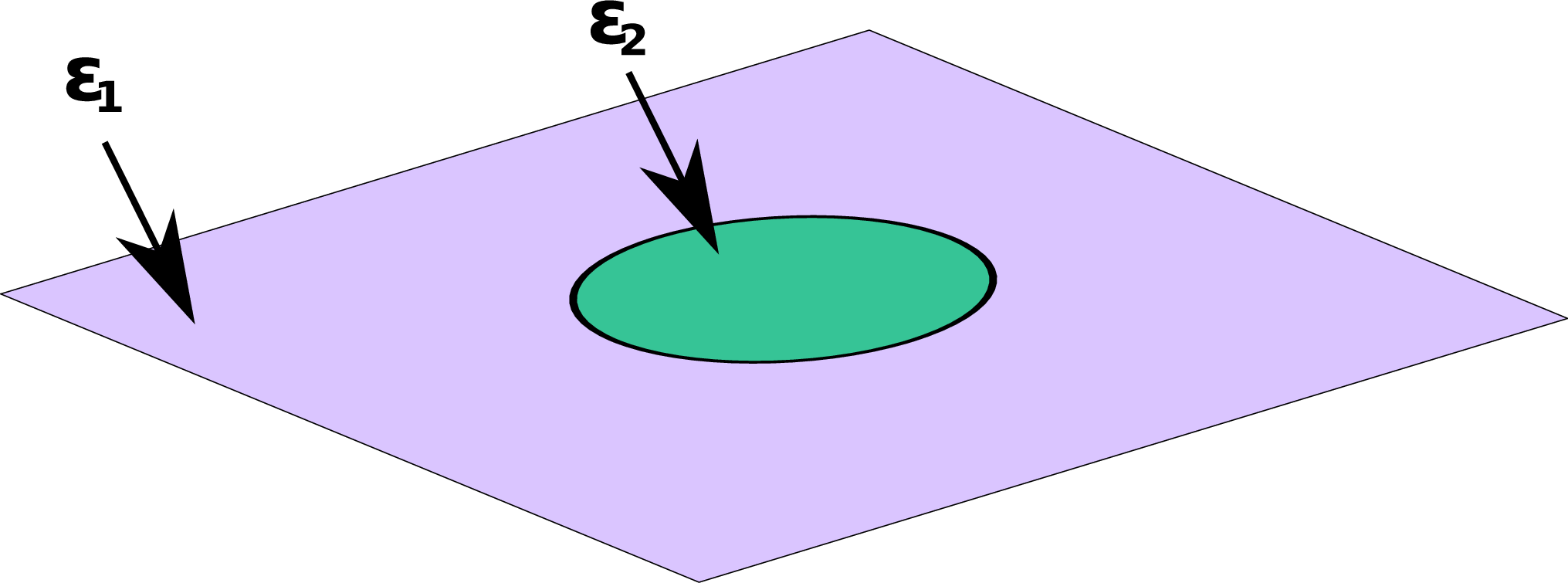
The action (6) is an effective low-energy expression in the sense that it only describes the ‘stringy’ variables and is applicable as long as the effects of thickness of the string and of its internal structure can be neglected. Denoting the mass scale at which such approach becomes invalid (e.g. the thickness of the string ), one can write the condition for the applicability of the effective action (6) in terms of the length scale, , and the momentum scale . Assuming that the initial very long string with tension is located along the axis, one can readily find that the action (6) has a nontrivial stationary configuration, the bounce, namely, that of a disk in the (t,x) plane occupied by the phase , as shown in Fig.1, with the radius
| (7) |
which is the radius (one half of the length) of the critical gap. The difference between the action (6) on this configuration and on the trivial one is exactly the expression for the exponential power in Eq.(1), and the condition for applicability of the effective action (6) requires
| (8) |
Generally one also has , and for the strings in weakly coupled theories , so that the power in the exponent in Eq.(1) is large, which justifies a semiclassical treatment.
The probability of the transition is determined[8, 5, 7] by (the imaginary part of) the ratio of the path integrals and calculated with the action (6) around respectively the bounce configuration and around the initial flat string:
| (9) |
It can also be reminded that, as explained in great detail in Ref.[7], that the imaginary part of arises from one negative mode at the bounce configuration, and that due to two translational zero modes the numerator in Eq.(9) is proportional to the total space time area in the plane occupied by the string, so that the finite quantity is the transition probability per unit time (the rate) and per unit length of the string.
In order to evaluate the relevant path integrals with the pre-exponential accuracy we use the cylindrical coordinates, with and being the polar variables in the plane (of the bounce), and being the transverse coordinate. We consider only one transverse coordinate, since the effect of each of the extra dimensions factorizes, so that the corresponding generalization is straightforward. We further assume, for definiteness, that the space-time boundary in the plane is a circle of large radius , where the boundary condition for the string is . The small deviations of the string configuration from the bounce, illustrated in Fig.2, can be parametrized by the radial () and transverse () shifts of the boundary between the string phases:
| (10) |
and the variations of the surfaces of the two string phases: and , where, naturally,
| (11) |

In terms of these variables the action (6) can be written in the quadratic approximation in the deviations from the bounce as
| (12) |
where the primed and dotted symbols stand for the derivatives with respect to and correspondingly.
Finally, the action around a flat initial string configuration in the quadratic approximation takes the form
| (13) |
with parametrizing small deviations of the string in the transverse direction.
3 Separating variables in the path integrals
One can readily see that in the quadratic part of the action (12) the ‘longitudinal’ variation of the bounce boundary in the plane, described by the function completely decouples from the rest of the variables. This implies that the path integral over can be considered independently of the integration over other variables and that it enters as a factor in . On the other hand it is this integral that provides the imaginary part to the partition function, and it is also proportional to the total space-time area . Moreover, this path integral is identical to the one entering the problem of false vacuum decay in (1+1) dimensions and we can directly apply the result of that calculation[10]:
| (14) |
The expression for the transition rate thus can be written in the form
| (15) |
with the path integral running only over the transverse variables , and ,
| (16) |
and involving only the quadratic in these variables part of the action (12),
| (17) |
In the same quadratic approximation the flat string partition function is given by
| (18) |
with given by Eq.(13) and the integral running over all the functions vanishing at the space-time boundary: .
At this point there still is a coupling in the path integral (16) between the bulk variables , and the boundary variable arising from the boundary conditions (11). This however is a simple issue which is resolved by a straightforward shift of the integration variables and . Namely, we write
| (19) |
where and are the new integration variables in and these functions satisfy zero boundary conditions,
| (20) |
while and are fixed (for a fixed ) functions satisfying the boundary conditions
| (21) |
which are also harmonic, i.e. satisfying the Laplace equation .
After the specified shift of the variables we arrive at the expression for the action (17) in which the bulk and the boundary degrees of freedom are fully separated:
| (22) | |||||
Clearly, the boundary terms in the first line here, arising from the integration by parts, depend only on the transverse shift of the boundary . The partition function can thus be written as a product of the ‘boundary’ and the ‘bulk’ terms:
| (23) |
with the being given by the path integral over the bulk variables and only :
| (24) |
and the boundary term
| (25) |
involving integration over only the boundary values.
The subsequent calculation of the ratio of the partition functions in Eq.(15) can in fact be reduced to a calculation of only. In order to achieve this reduction one should organize the partition function in the denominator of Eq.(15) in a form similar to Eq.(23) as follows. Although the flat string configuration makes no reference to a circle of the radius , the partition function can be calculated by first fixing the transverse variable at : and separating the integration over the bulk variables. Then the flat string partition function factorizes in the form similar to Eq.(23):
| (26) |
with given a similar path integral as in Eq.(24),
| (27) |
where, as in Eq.(24), and are respectively the outer (i.e. at ) and the inner () transverse fluctuations with zero boundary conditions. The difference in the coefficient in the expressions (24) and (27) for the contribution of the inner part, vs. , is not essential, since the overall coefficient of the quadratic part of the action is absorbed in the measure of integration, as can be seen by rescaling to the corresponding canonically normalized variables .
One therefore finds that , and the ratio of the partition functions in Eq.(15) is in fact determined by the ratio of the boundary terms.
4 Regularization
The boundary factor for the flat string is somewhat different from the one given by Eq.(25) and reads as
| (28) |
where the functions and are defined in the same way as in Eq.(25).
The latter functions can be readily found by expanding the boundary function in angular harmonics:
| (29) |
with and being the amplitudes of the harmonics. Then at the harmonics of the discussed functions are found as
| (30) |
and for n=0 these are given by
| (31) |
Substituting these expressions for the harmonics in the equations (25) and (28) and performing the Gaussian integration over the amplitudes and we find the boundary factors in the form
| (32) |
and
| (33) |
with being a normalization factor.
Clearly, each of the formal expressions (32) and (33) contains a divergent product, and their ratio is also ill defined, so that our calculation requires a regularization procedure that would cut off the contribution of harmonics with large . A regularization of high harmonics is also required on general grounds. Indeed, as previously mentioned, our consideration using the effective string action (6) is only valid for smooth deformations of the string, i.e. as long as the relevant momenta are smaller than the mass scale for excitation of the internal degrees of freedom within the thickness of the string. For an -th harmonic the relevant momentum is so that the applicability of the effective low energy action requires a cutoff at . In order to perform such regularization we use the standard Pauli-Villars method and introduce a regulator field with negative norm and the action corresponding to the quadratic part of the Nambu-Goto expression (6) for small :
| (34) |
with being the regulator mass, which physically should be understood as satisfying the condition and still being much larger than the relevant scale in the discussed problem, in particular .
The regularized expression for the ratio of the boundary terms in and thus takes the form
| (35) |
where we introduced the notation for the regularized ratio, and the regulator partition functions and are determined by the same expressions as in Eqs.(25) and (28) with the ‘outer’ and ‘inner’ functions and being replaced by their regulator counterparts and which still satisfy the boundary conditions similar to (21):
| (36) |
but are the solutions of the Helmholtz rather than Laplace equation .
The solutions of the latter equation fall off exponentially at the scale determined by , and for our purposes only the behavior near the circle is needed. For this reason we write the equation for the radial part of the -th angular harmonic ,
| (37) |
and parametrize the radial coordinate as , and treat the parameter as small, since the scale for the variation of the solution is . This approach yields an expansion of the regulator action associated with the boundary at in powers of . With the accuracy required in the present calculation, the (normalized to one at ) solution to Eq.(37) is found in the first order of expansion in as
| (38) |
Using the form of the solutions for the harmonics of the regulator field given by Eq.(38) and the expressions (32) and (33), one can write the regularized ratio of the boundary partition functions (35) as
| (39) | |||||
where we introduced the notation
| (40) |
and the last product factor in Eq.(39) arises from the first term of expansion in in the pre-exponential factor in Eq.(38)
5 Calculating the products
Each of the products in Eq.(39) is finite at a finite and can be calculated separately. We start with the most straightforward one, which is directly given by an Euler’s formula:
| (41) |
where the last transition corresponds to the limit .
The other two factors in Eq.(39), the first and the last, generally depend on the relation between the parameters and , or equivalently between and . We find however that the latter product is equal to one at independently of . In particular in the nontrivial case of we find
| (42) |
where the lower limit in the integral is any number that is finite in the limit .
The dependence of the first product factor in Eq.(39) on the ratio is essential and we consider two limiting cases when this ratio is much bigger than one and when it is very small. In the former case, i.e. for , the first product in Eq.(39) becomes reciprocal of the second, and one finds
| (43) |
(Clearly one can also safely make the replacement at .)
The behavior of in the opposite limit, i.e. at , turns out to be significantly more interesting. Using the Euler-Maclaurin summation formula for the logarithm of the first product in Eq.(39) we find in the limit and :
| (44) |
Being combined with the expression (42) this yields the formula
| (45) |
which contains an essential dependence on the regulator mass parameter . We will show however that all such dependence in the phase transition rate can be absorbed in renormalization of the parameter in the leading semiclassical term.
6 Renormalization of
The parameter is defined in the action (6) as the coefficient in front of the length of the boundary between the world sheets for two phases of the string. Generally this parameter gets renormalized by the quantum corrections, and in order to find such renormalization at the level of first quantum corrections, one needs to perform the path integration using the quadratic part of the action around a configuration, in which the length of the interface is an arbitrary parameter. For a practical calculation of this effect we consider a Euclidean space configuration, shown in Fig.3, with the string lying flat along the axis, and the interface between the two phases being at . The length of the world line for the boundary is thus the total size of the world sheet in the time direction. It should be mentioned that such configuration with different string tension on each side of the boundary is not stationary for the action (6). However it can be ‘stabilized’ by a source term (external force) depending on the coordinate of the boundary: , which term does not affect the quadratic in fluctuations part of the action.

The Gaussian path integral over the transverse coordinates is then to be calcite with the zero boundary conditions at the edges of the total world sheet. Using the notation for the transverse shift of the boundary, this condition implies , so that the function has the Fourier expansion of the form
| (46) |
and a similar expansion applies to the regulator boundary function . The part of the effective action associated with the boundary is determined by the functions for the transverse shift of the string and the corresponding regulator functions that satisfy the equations
| (47) |
and the boundary conditions
| (48) |
as well as zero boundary conditions at the edges of the total world sheet. One can readily find these functions for each harmonic of the boundary values and , using the normalized to one solutions for and in each harmonic:
| (49) |
and
| (50) |
In order to separate the boundary effect in the path integral around the considered configuration from the bulk effects, we again divide it by the path integral around the configuration where the whole world sheet is occupied by the same phase of the string. The latter phase can be chosen with either of the tensions, or with an arbitrary tension . Such division results, as previously, in the cancellation of the bulk contributions, and the remaining part of the effective action associated with the boundary is written in terms of the regularized path integral over the boundary function as
| (51) |
where is the renormalized mass parameter. The correction to can thus be written in the form
| (52) |
where
| (53) |
In the limit one can directly apply the results in Eqs.(41) and (44) for evaluation of the expression (52) and write
| (54) | |||||
where a use is made of the Stirling formula
considering that is proportional to large .
In the limiting case where the correction vanishes, so that the renormalization effect is negligible.
7 The result and discussion
We can now assemble all the relevant elements into a formula for the rate of the considered transition. Clearly, the path integration over the variables factorizes for each of the transverse dimensions, so that the expression for the decay rate takes the form
| (55) |
where is the zeroth order mass parameter. In the case of large string tension, , the ‘bare’ coincides with the renormalized one, and the factor is equal to one. It can be noted that the resulting obvious expression for the rate is also correctly given by Eq.(4) as soon as the factor in Eq.(5) is taken in the limit : , which limit, as previously discussed, is mandated in this case.
In the opposite limit of heavy , , both the expression (45) depends on the regulator mass and the -dependent renormalization of is essential. Taking into account that each of the transverse dimensions contributes additively to and expressing in Eq.(55) the bare through the renormalized one: , one readily finds that the dependence on the regulator mass M cancels in the transition rate, and one arrives at the formula given by Eq.(4) and Eq.(5).
The formula (5) is applicable for arbitrary ratio of the string tensions . In particular it can be also applied at , in which case the considered transition describes a complete breaking of the string.
It can be also noted that numerically the factor depends very moderately on the ratio of the tensions and changes approximately linearly between and . We thus conclude that the two-dimensional expression (3) for the pre-exponential factor in the transition rate provides a fairly accurate approximation in higher dimensions as well, as long as the exponential factor is expressed in terms of the physical renormalized mass .
There is however an interesting methodical point pertaining to the considered here problem. Indeed, as was already mentioned, the difference from the problem of particle creation by external electric field is that the motion of the ends of the string involves in addition to the mass also an adjacent part of the string. In terms of the calculation of the path integrals around the bounce the difference is that the spectrum of soft modes in the particle creation problem (as well as in that of the two-dimensional false vacuum decay) consists only of the modes associated with one-dimensional world line of the boundary of the bounce. The entire pre-exponential factor can then be found using the effective low energy action for these modes[10]. In the considered here string transition there are also low modes in the bulk of the world sheet of the string, and there is no parametric separation of their eigenvalues from those of the modes associated with fluctuations of the boundary. In the presented calculation the separation of the boundary and bulk variables is achieved through an ‘artificial’ organization of the normalization partition function for a flat string into boundary and bulk factors and . The bulk contribution then cancels in the ratio of the partition functions near the bounce and near a flat string, so that the remaining calculation is reduced to considering the integrals over the boundary functions only. One can also readily notice that the additional contribution to the action from the boundary terms as e.g. those with the functions and in Eq.(25) corresponds to precisely the effect of ‘dragging’ of the string by its end.
Acknowledgment
The work of M.B.V. is supported in part by the DOE grant DE-FG02-94ER40823.
References
- [1] A. Vilenkin, Nucl. Phys. B 196, 240 (1982).
- [2] J. Preskill and A. Vilenkin, Phys. Rev. D 47, 2324 (1993) [arXiv:hep-ph/9209210].
- [3] M. Shifman and A. Yung, Phys. Rev. D 66, 045012 (2002) [arXiv:hep-th/0205025].
- [4] M. B. Voloshin, I. Y. Kobzarev and L. B. Okun, Sov. J. Nucl. Phys. 20, 644 (1975) [Yad. Fiz. 20, 1229 (1974)].
- [5] S. R. Coleman, Phys. Rev. D 15, 2929 (1977) [Erratum-ibid. D 16, 1248 (1977)].
- [6] J. Schwinger, Phys. Rev. 86, 664 (1951).
- [7] C. G. Callan and S. R. Coleman, Phys. Rev. D 16, 1762 (1977).
- [8] M. Stone, Phys. Rev. D 14, 3568 (1976).
- [9] V. G. Kiselev and K. G. Selivanov, JETP Lett. 39, 85 (1984) [Pisma Zh. Eksp. Teor. Fiz. 39, 72 (1984)].
- [10] M. B. Voloshin, Yad. Fiz. 42, 1017 (1985) [Sov. J. Nucl. Phys. 42, 644 (1985)].