Transverse momentum spectra of charged hadrons in jets at the Tevatron

The production of jets – a collimated bunch of hadrons – in $e^{+}e^{-}$, $e^{-}p$ and hadronic collisions is an ideal playground to investigate the parton evolution process in perturbative QCD (pQCD). One of the great successes of pQCD is the existence of the hump-backed shape of inclusive spectra, predicted in [1] within MLLA, and later discovered experimentally (for review, see e.g. [2]). Refining the comparison of pQCD calculations with jet data taken at LEP, Tevatron and LHC will ultimately allow for a crucial test of the Local Parton Hadron Duality (LPHD) hypothesis [3] and for a better understanding of color neutralization processes.

The inclusive ${k_{{}_{\perp}}}$-distribution of particles inside a jet has been computed at MLLA accuracy in the limiting spectrum approximation [4], i.e. assuming an infrared cutoff $Q_{0}$ equal to $\Lambda_{{}_{{}_{\rm QCD}}}$ ($\lambda\equiv\ln(Q_{0}/\Lambda_{{}_{{}_{\rm QCD}}})=0$) (for a review, see also [5]). MLLA corrections, of relative magnitude ${{\cal{O}}}\left(\sqrt{\alpha_{s}}\right)$ with respect to the leading double logarithmic approximation (DLA), were shown to be quite substantial [4]. Therefore, it appears legitimate to wonder whether corrections of order ${{\cal{O}}}\left(\alpha_{s}\right)$, that is next-to-next-to-leading or Next-to-MLLA (NMLLA), are negligible or not.

The starting point of this analysis is the MLLA Master Equation for the Generating Functional (GF) $Z=Z(u)$ of QCD jets [5], where $u=u(k)$ is a certain probing function and $k$, the four-momentum of the outgoing parton. Together with the initial condition at threshold, the GF determines the jet properties at all energies. For instance, the single inclusive spectrum can be derived from the GF by differentiating with respect to $u=u(k)$, and the solution of the equations can be written as a perturbative expansion in $\sqrt{\alpha}_{s}$. At high energies this expansion can be resummed and the leading contribution be represented as an exponential of the anomalous dimension $\gamma(\alpha_{s})$. Since further details to this logic can be found in [5, 6], we only give the symbolic structure of the equation for the GF and its solution, which we write respectively as

where $\gamma(\alpha_{s})$ can be expressed as a power series of $\sqrt{\alpha}_{s}$

In this logic, the leading (DLA, ${\cal O}(\sqrt{\alpha_{s}})$) and next-to-leading (MLLA, ${\cal O}(\alpha_{s})$) approximations are complete. The next terms (NMLLA, ${\cal O}(\alpha_{s}^{3/2})$) are not complete but they include an important contribution which takes into account energy conservation and an improved behavior near threshold. Indeed, some results for such NMLLA terms have been studied previously for global observables and have been found to better account for recoil effects and to drastically affect multi-particle production [7, 8].

The equation in (1) applies to each vertex of the cascade and its solution represents the fact that successive and independent partonic splittings inside the shower, exponentiate with respect to the evolution-time parameter $dy=d\Theta/\Theta$, where $\Theta\ll 1$ is the angle between outgoing couples of partons. The choice of $y$ follows from Angular Ordering (AO) in intra-jet cascades. It is indeed the suited variable for describing time-like evolution in jets. Thus, Eq. (1) incorporates the Markov chains of sequential angular ordered partonic decays which are singular in $\Theta$ and $\gamma(\alpha_{s})$ determines the real rate of inclusive quantities growth with energy.

While DLA treats the emission of both particles as independent by keeping track of the first term $\sim\sqrt{\alpha}_{s}$ in (2) without constraint, the exact solution of the MLLA evolution equation (partially) fulfills the energy conservation in each individual splitting process ($z+(1-z)=1$) by incorporating higher order ($\alpha_{s}^{n/2},n>1$) terms to the anomalous dimension. Symbolically, the first two analytical steps towards a better account of these corrections in the MLLA, NMLLA evolution, which we further discuss in [9], can be represented in the form

where $\ell=\ln(1/x)\sim\alpha_{s}^{-1/2}$ with $x\ll 1$ (fraction of the jet energy taken away by one hadron), $z\sim 1$ for hard partons splittings such as $g\to q\bar{q}$…(this is in fact the region where the two partons are strongly correlated).

Energy conservation is particularly important for energetic particles as the remaining phase space is then very limited. On the other hand, a soft particle can be emitted with little impact on energy conservation. Some consequences of this behavior have also been noted in [10]:

• $(i)$

  the soft particles follow the features expected from DLA;

• $(ii)$

  there is no energy dependence of the soft spectrum;

• $(iii)$

  the ratio of soft particles $r=N_{g}/N_{q}$ in gluon and quark jets is consistent with the DLA prediction $N_{c}/C_{F}=9/4$ (see the measurement by DELPHI [11]).

The present study makes use of this logic (3) to evaluate NMLLA contributions to the single inclusive $k_{\perp}$-distribution. The main results of this work have been published in [9, 12]. Experimentally, the CDF collaboration at the Tevatron reported on ${k_{{}_{\perp}}}$-distributions of unidentified charged hadrons in jets produced in $p\bar{p}$ collisions at $\sqrt{s}=1.96$ TeV [13].

We start by writing the MLLA evolution equations for the fragmentation function $D_{B}^{h}\left(x\big/z,zE\Theta_{0},Q_{0}\right)$ of a parton B (energy $zE$ and transverse momentum ${k_{{}_{\perp}}}=zE\Theta_{0}$) into a gluon (represented by a hadron $h$ (energy $xE$) according to LPHD [3]) inside a jet A of energy $E$ for the process depicted in Fig. 1.

As a consequence of angular ordering in parton cascading, partonic distributions inside a quark and gluon jet, $Q,G(z)=x\big/z\ D_{Q,G}^{h}\left(x\big/z,zE\Theta_{0},Q_{0}\right)$, obey the system of two coupled equations [6] (the subscript _y denotes $\partial/\partial{y}$) following from the MLLA master equation described by (1)

$\Phi_{A}^{B}(z)$ denotes the Dokshitzer-Gribov-Lipatov-Altarelli-Parisi (DGLAP) splitting functions [5],

where $\phi_{q}^{g}(z)=z-2$ and $\phi_{g}^{g}(z)=(z-1)(2-z(1-z))$ are regular as $z\to 0$, $C_{F}=(N_{c}^{2}-1)/2N_{c}$, $T_{R}=n_{f}/2$ ($N_{c}=3$ is the number of colors for $SU(3)_{c}$ and $n_{f}=3$ is the number of light flavors we consider). The running coupling of QCD ($\alpha_{s}$) is given by

and

where $Q_{0}$ is the collinear cut-off parameter. Moreover,

At small $x\ll z$, the fragmentation functions behave as

$\rho_{B}^{h}$ being a slowly varying function of two logarithmic variables $\ln(z/x)$ and $y$ that describes the “hump-backed” plateau. Since recoil effects should be largest in hard parton splittings, the strategy followed in this work is to perform Taylor expansions (first advocated for in [15]) of the non-singular parts of the integrands in (4,5) in powers of $\ln z$ and $\ln(1-z)$, both considered small with respect to $\ell$ in the hard splitting region $z\sim 1-z={{\cal{O}}}\left(1\right)$

Each $\ell$-derivative giving an extra $\sqrt{\alpha_{s}}$ factor (see [6]), the terms $B_{\ell}(1)\ln z$ and $B_{\ell}(1)\ln\left(1-z\right)$ yield NMLLA corrections to the solutions of (5). Making used of (6), after integrating over the regular parts of the DGLAP splitting functions, while keeping the singular terms unchanged, one gets after some algebra ($\gamma_{0}^{2}=2N_{c}\alpha_{s}/\pi$) [9, 12]

with $\psi_{\ell}(\ell,y)=G_{\ell}(\ell,y)/G(\ell,y)$. The MLLA coefficients
${\tilde{a}_{1}=3/4}$ and $a_{1}\approx 0.935$ are computed in [6] while at NMLLA, we get

Defining $F(\ell,y)=\gamma_{0}^{2}(\ell+y)G(\ell,y)$, we can exactly solve the self-contained equation (8) by performing the Mellin transform

Inserting (11) into (8) we obtain, after some algebra, the differential equation

Finally, after inserting the solution of (12) into (11), the new integral representation for the inclusive spectrum (hump-backed plateau) with NMLLA accuracy reads

where

However, computing (13) numerically is quite a challenging task. As can be seen, the NMLLA coefficient $a_{2}$ is very small. This may explain a posteriori why the MLLA “hump-backed plateau” agrees very well with experimental data [1, 14]. Therefore, the NMLLA solution (13) of (8) can be approximated by the MLLA solution of $G(\ell,y)$ (i.e. taking $a_{2}\approx 0$), which will be used in the following to compute the inclusive ${k_{{}_{\perp}}}$-distribution. As demonstrated in [6], taking the limits $a_{2}\approx 0$ and $\lambda\approx 0$ in (13), the integral representation can be reduced to the known MLLA formula [5]

where the integration is performed with respect to $\tau$ defined by $\displaystyle\alpha=\frac{1}{2}\ln\frac{y}{\ell}+i\tau$ and with

$B=a_{1}/\beta_{0}$ and $I_{B}$ is the modified Bessel function of the first kind. To get a quantitative idea on the difference between MLLA and NMLLA gluon inclusive spectrum, the reader is reported to the appendix B of [9]. The magnitude of $\tilde{a}_{2}$, however, indicates that the NMLLA corrections to the inclusive quark jet spectrum may not be negligible and should be taken into account. After solving (8), the solution of (7) reads

It differs from the MLLA expression given in [4] by the term proportional to $G_{\ell\ell}$, which can be deduced from the subtraction of $(C_{F}/N_{c})\times$(8) to Eq. (7).

Computing the single inclusive $k_{\perp}-$ distribution requires the definition of the jet axis. The starting point of our approach consists in considering the correlation between two particles (h1) and (h2) of energies $E_{1}$ and $E_{2}$ which form a relative angle $\Theta$ inside one jet of total opening angle $\Theta_{0}>\Theta$ [16]. Weighting over the energy $E_{2}$ of particle (h2), this relation leads to the correlation between the particle (h=h1) and the energy flux, which we identify with the jet axis (see Fig. 2) [4]. Thus, the correlation and the relative transverse momentum $k_{\perp}$ between (h1) and (h2) are replaced by the correlation, and transverse momentum of (h1) with respect to the direction of the energy flux. Finally, we obtain the double differential spectrum ${\rm d}^{2}N/{\rm d}{x}\,{\rm d}\Theta$ of a hadron produced with energy $E_{1}=xE$ at angle $\Theta$ (or $k_{\perp}\approx xE\Theta$) with respect to the jet axis. As demonstrated in [4], the correlation reads

where $F_{A_{0}}^{h}$ is given by the convolution of two fragmentation functions

$u$ being the energy fraction of the intermediate parton $A$. $D_{A_{0}}^{A}$ describes the probability to emit $A$ with energy $uE$ off the parton $A_{0}$ (which initiates the jet), taking into account the evolution of the jet between $\Theta_{0}$ and $\Theta$. $D_{A}^{h}$ describes the probability to produce the hadron $h$ off $A$ with energy fraction $x/u$ and transverse momentum ${k_{{}_{\perp}}}\approx uE\Theta\geq Q_{0}$ (see Fig. 2).

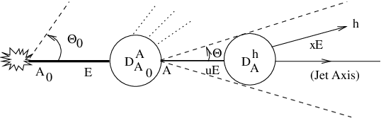
As discussed in [4], the convolution (17) is dominated by $u\sim 1$ and therefore $D_{A_{0}}^{A}\left(u,E\Theta_{0},uE\Theta\right)$ is determined by the DGLAP evolution [5]. On the contrary, the distribution $D_{A}^{h}\left(\frac{x}{u},uE\Theta,Q_{0}\right)$ at low $x\ll u$ reduces to the hump-backed plateau,

with $Y_{\Theta}=\ell+y=\ln E\Theta/Q_{0}$. Performing the Taylor expansion of $\tilde{D}$ to the second order in $(\ln u)$ and plugging it into Eq. (17) leads to

Indeed, since soft particles are less sensible to the energy balance, the correlation (17) is proved to disappear for these particles, leading to the sequence of factorized terms written in (19). The first two terms in Eq. (19) correspond to the MLLA distribution calculated in [4] when $\tilde{D}_{A}^{h}$ is evaluated at NLO and its derivative at LO. NMLLA corrections arise from their respective calculation at NNLO and NLO, and, mainly in practice, from the third line, which was computed in [9, 12]. Indeed, since $x/u$ is small, the inclusive spectrum $\tilde{D}_{A}^{h}(\ell,y)$ with $A=G,Q$ are given by the solutions (13) and (15) of the next-to-MLLA evolution equations (7) and (8) respectively. However, because of the smallness of the coefficient $a_{2}$ (see (10)), $G(\ell,y)$ shows no significant difference from MLLA to NMLLA. As a consequence, we use the MLLA expression (14) for $G(\ell,y)$, and the NMLLA (15) for $Q(\ell,y)$. The functions $F_{g}^{h}$ and $F_{q}^{h}$ are related to the gluon distribution via the color currents $\langle C\rangle_{g,q}$ defined as:

$\langle C\rangle_{g,q}$ can be seen as the average color charge carried by the parton $A$ due to the DGLAP evolution from $A_{0}$ to $A$. Introducing the first and second logarithmic derivatives of $\tilde{D}_{A}^{h}$,

Eq. (19) can now be written as

with the notation

The scaling violation of the DGLAP fragmentation function neglected in the last approximation is a NMLLA correction to $<u>$. It however never exceeds $5\%$ [9] of the leading contribution and is thus neglected in the following. Using (20), the MLLA and NMLLA corrections to the leading color current of the parton $A_{0}=g,q$ read

The MLLA correction, ${{\cal{O}}}\left(\sqrt{\alpha_{s}}\right)$, was determined in [4] and the NMLLA contribution, ${{\cal{O}}}\left(\alpha_{s}\right)$, to the average color current is new. The latter can be obtained from the Mellin moments of the DGLAP fragmentation functions

leading to

Plugging (23) into the resummed expression $<C>_{g,q}$ of the color current as written in (20), these quantities for gluon and quark jets are determined analytically [9]. For illustrative purposes, the LO, MLLA, and NMLLA average color current of a quark jet with $Y_{\Theta_{0}}=6.4$ – corresponding roughly to Tevatron energies – is plotted in Fig. 3 as a function of $y$, at fixed $\ell=2$ for $\lambda\approx 0$. As discussed in [4], the MLLA corrections to the LO color current are found to be large and negative. As expected, the correction ${{\cal{O}}}\left(\alpha_{s}\right)$ from MLLA to NMLLA proves much smaller; it is negative (positive) at small (large) $y$.

This calculation has also been extended beyond the limiting spectrum, $\lambda\neq 0$, to take into account hadronization effects in the production of “massive” hadrons, $m={{\cal{O}}}\left(Q_{0}\right)$ [18]. We used, accordingly, the more general MLLA solution of (8) with $a_{2}=0$ for an arbitrary $\lambda\neq 0$

from which an analytic approximated expression was found using the steepest descent method [17]; $\sigma_{2}=0$ and $\sigma_{3}=\lambda$ have been set in (13). However, $G(\ell,y)$ is here determined exactly from an equivalent representation in terms of a single Mellin transform (which reduces to (14) as $\lambda\to 0$) [18]

which is better suited for numerical studies. The function ${\cal K}$ appearing in Eq. (24) reads

where $A=1/(\beta_{0}\ \omega)$, $B=a_{1}/\beta_{0}$, and $\Phi$ and $\Psi$ are the confluent hypergeometric function of the first and second kind, respectively. The NMLLA (normalized) corrections to the MLLA result are displayed in Fig. 4 for different values $\lambda=0,0.5,1$, by using (24). It clearly indicates that the larger $\lambda$, the smaller the NMLLA corrections. In particular, they can be as large as $30\%$ at the limiting spectrum ($\lambda=0$) but no more than $10\%$ for $\lambda=0.5$. This is not surprising since $\lambda\neq 0$ ($Q_{0}\neq\Lambda_{{}_{{}_{\rm QCD}}}$) reduces the parton emission in the infrared sector and, thus, higher-order corrections.

The double differential spectrum
$({\rm d}^{2}N/{\rm d}\ell\,{\rm d}{y})$, Eq. (16), can now be determined from the NMLLA color currents (22) using the MLLA quark and gluon distributions. Integrating it over $\ell$ leads to the single inclusive $y$-distribution (or ${k_{{}_{\perp}}}$-distribution) of hadrons inside a quark or a gluon jet:

where

is the explicit expression of the double differential distribution (16). The MLLA framework does not specify down to which values of $\ell$ (up to which values of $x$) the double differential spectrum $({\rm d}^{2}N/{\rm d}\ell\,{\rm d}{y})$ should be integrated over. Since $({\rm d}^{2}N/{\rm d}\ell\,{\rm d}{y})$ becomes negative (non-physical) at small values of $\ell$ (see e.g. [4]), we chose the lower bound $\ell_{\rm min}$ so as to guarantee the positiveness of $({\rm d}^{2}N/{\rm d}\ell\,{\rm d}{y})$ over the whole $\ell_{\rm min}\leq\ell\leq Y_{\Theta_{0}}$ range (in practice, $\ell_{\rm min}^{g}\sim 1$ and $\ell_{\rm min}^{q}\sim 2$). Having successfully computed the single ${k_{{}_{\perp}}}$-spectra including NMLLA corrections, we now compare the result with existing data. The CDF collaboration at the Tevatron recently reported on preliminary measurements over a wide range of jet hardness, $Q=E\Theta_{0}$, in $p\bar{p}$ collisions at $\sqrt{s}=1.96$ TeV [13]. CDF data, including systematic errors, are plotted in Fig. 5 together with the MLLA predictions of [4] and the present NMLLA calculations, both at the limiting spectrum ($\lambda=0$) and taking $\Lambda_{{}_{{}_{\rm QCD}}}=250$ MeV; the experimental distributions suffering from large normalization errors, data and theory are normalized to the same bin, $\ln({k_{{}_{\perp}}}/1\,\text{GeV})=-0.1$.

The agreement between the CDF results and the NMLLA distributions over the whole ${k_{{}_{\perp}}}$-range is particularly good. In contrast, the MLLA predictions prove reliable in a much smaller ${k_{{}_{\perp}}}$ interval. At fixed jet hardness (and thus $Y_{\Theta_{0}}$), NMLLA calculations prove accordingly trustable in a much larger $x$ interval. Despite this encouraging agreement with data, the present calculation still suffers from certain theoretical uncertainties, discussed in detail in [9]. Among them, the variation of $\Lambda_{{}_{{}_{\rm QCD}}}$ –giving NMLLA corrections– from the default value $\Lambda_{{}_{{}_{\rm QCD}}}=250$ MeV to $150$ MeV and $400$ MeV affects the normalized ${k_{{}_{\perp}}}$-distributions by roughly $20\%$ in the largest $\ln({k_{{}_{\perp}}}/1\penalty\ \text{GeV})=3\penalty\ \text{GeV}$-bin at $Q=100$ GeV. Also, cutting the integral (26) at small values of $\ell$ is somewhat arbitrary. However, we checked that changing $\ell_{min}$ from $1$ to $1.5$ modifies the NMLLA spectra at large ${k_{{}_{\perp}}}$ by $\sim 20\%$ only ¹¹ 1 The effect of varying $\ell_{min}$ is more dramatic at MLLA.. Finally, the kt-distribution is determined with respect to the jet energy flow (which includes a summation over secondary hadrons in energy-energy correlations). In experiments, instead, the jet axis is determined exclusively from all particles inside the jet. The question of the matching of these two definitions goes beyond the scope of this letter. The NMLLA ${k_{{}_{\perp}}}$-spectrum has also been calculated beyond the limiting spectrum, by plugging (24) into (26), as illustrated in Fig. 6. However, the best description of CDF preliminary data is reached at the limiting spectrum, or at least for small values of $\lambda\lesssim 0.5$, which is not too surprising since these inclusive measurements mostly involve pions. Identifying produced hadrons would offer the interesting possibility to check a dependence of the shape of ${k_{{}_{\perp}}}$-distributions on the hadron species, such as the one predicted in Fig. 6.

Moreover, the softening of the ${k_{{}_{\perp}}}$-spectra with increasing hadron masses predicted in Fig. 6 is an observable worth to be measured, as this would provide an additional and independent check of the LPHD hypothesis beyond the limiting spectrum. This could only be achieved if the various species of hadrons inside a jet can be identified experimentally. Fortunately, it is likely to be the case at the LHC, where the ALICE [19] and CMS [20] experiments at the Large Hadron Collider have good identification capabilities at not too large transverse momenta.

To summarize, single inclusive ${k_{{}_{\perp}}}$-spectra inside a jet are determined including higher-order ${{\cal{O}}}\left(\alpha_{s}\right)$ (i.e. NMLLA) corrections from the Taylor expansion of the MLLA evolution equations and beyond the limiting spectrum, $\lambda\neq 0$. The agreement between NMLLA predictions and CDF preliminary data in $p\bar{p}$ collisions at the Tevatron is impressive, indicating very small overall non-perturbative corrections and giving further support to LPHD [3]. The MLLA evolution equations for inclusive enough variables prove once more (see e.g. [5]) to include reliable information at higher orders than MLLA.

References

- (1)
Yu.L. Dokshitzer, V.S. Fadin, V.A. Khoze, Phys. Lett. B 115 (1982) 242;
Ya.I. Azimov, Yu.L. Dokshitzer, V.A. Khoze, S.I. Troian, Z. Phys. C 31 (1986) 213;
C.P. Fong, B.R. Webber, Phys. Lett. B 229 (1989) 289. - (2) V.A. Khoze, W. Ochs, Int. J. Mod. Phys. A 12 (1997) 2949.
- (3)
Ya.I. Azimov, Yu.L. Dokshitzer,
Z. Phys C 27 (1985) 65;
Yu.L. Dokshitzer, V.A. Khoze, S.I. Troian, J. Phys. G 17 (1991) 1585. - (4) R. Pérez Ramos, B. Machet, JHEP 04 (2006) 043.
- (5) Yu.L. Dokshitzer, V.A. Khoze, A.H. Mueller, S.I. Troyan, (Editions Frontières, Gif-sur-Yvette, 1991).
- (6) R. Pérez Ramos, JHEP 06 (2006) 019 and references therein.
- (7) Yu.L. Dokshitzer, Phys. Lett. B 305 (1993) 295.
- (8) F. Cuypers, K. Tesima, Z. Phys. C 54 (1992) 87.
- (9) R. Perez-Ramos, F. Arléo & B. Machet, Phys. Rev. D 78 (2008) 014019.
- (10) V.A. Khoze, S. Lupia, W. Ochs, Phys. Lett. B 386 (1996) 451.
- (11) DELPHI Collaboration: J. Abdallah et al., Phys. Lett. B 605 (2005) 37.
- (12) F. Arleo, R. Pérez-Ramos, B. Machet, Phys. Rev. Lett. 100 (2008) 052002.
- (13) S. Jindariani, A. Korytov & A. Pronko, CDF report CDF/ANAL/JET/PUBLIC/8406 (March 2007), www-cdf.fnal.gov/physics/new/qcd/ktdistributions _06/cdf8406_Kt_jets_public.ps.
- (14) Yu.L. Dokshitzer, V.S. Fadin, V.A. Khoze, Z. Phys C 18 (1983) 37.
- (15)
I.M. Dremin, Phys. Usp. 37 (1994) 715;
ibid., Usp. Fiz. Nauk 164 (1994) 785;
I.M. Dremin, J.W. Gary, Phys. Rep. 349 (2001) 301;
I.M. Dremin, V.A. Nechitailo, Mod. Phys. Lett. A9 (1994) 1471. - (16) Yu.L. Dokshitzer, D.I. Dyakonov & S.I. Troyan, Phys. Rep. 58 (1980) 270.
- (17) R. Pérez Ramos, JHEP 09 (2006) 014.
- (18)
Yu.L. Dokshitzer, V.A. Khoze, S.I. Troian, Z. Phys. C 55 (1992) 107;
Yu.L. Dokshitzer, V.A. Khoze, S.I. Troian, Int. J. Mod. Phys. A 7 (1992) 1875;
V.A. Khoze, W. Ochs, J. Wosieck, and references therein. - (19) ALICE collaboration, J. Phys. G32 (2006) 1295.
- (20) CMS collaboration, D. d’Enterria (Ed.) et al., J. Phys. G34 (2007) 2307.