Parkinson’s Law Quantified:
Three Investigations on Bureaucratic Inefficiency

C.N. Parkinson has studied socio-dynamical systems with special focus on bureaucratic and administrative bodies. In his famous book [1] he comprises 10 essays which give detailed descriptions of microscopic mechanisms leading to macroscopic phenomena like exponential growth of administrations, impact on the size of executive councils on efficient decision-making, and the relationship between the age of retirement and a company’s vital promotion scheme. These essays are not quantitative, however, the description of these microscopic mechanisms is so clear and brilliant, that they can be easily cast into dynamical models. We pick three of these essays which are especially well suited for this purpose.

In the first essay (chapter 4 in [1]), Parkinson conjectured on historical evidence that there is a characteristic group size beyond which the ability of this group for efficient decision-making, i.e. the finding of consensus, is considerably diminished. The empirical findings based on government size, found in the 1950s [1], are still valid today to a large extend [15]. By proposing an opinion formation model for small groups we provide an understanding for this hypothesis through the existence of finite size effects which lead to this characteristic size (’Coefficient of Inefficiency’) of decision-making bodies.

In the second essay (chapter 1 in [1]), we formalize the so-called ’Parkinson’s Law’. We propose dynamical equations for his model of bureaucratic growth and solve them explicitly. As the main result we derive the phase diagram of this model for the macroscopic evolution of an administrative body. One phase corresponds to an exponentially growing body, the other to a shrinking one.

The third essay (chapter 10 in [1]), studies the interrelation between the age of retirement and promotion schemes with the motif force to ensure the presence of career opportunities and prevent the lack thereof, a phenomenon also known as ’Prince Charles Syndrome’. There we show the existence of a unique maximum for the efficiency of a bureaucratic body at the optimum life-time of a worker in the system. Given a promotion scheme and the hierarchy in the system, the optimal age of retirement can be computed.

This paper is organized as follows: in Section II we review work on the relationship between the size of a decision-making body and its efficiency [2]. In Section III we propose and solve the dynamical equations for a model of an administrative body which evolves according to Parkinson’s Law. The question when an official within such a body should retire to ensure a maximum of overall efficiency of the administrative body is left for the final Section IV. We interpret our results and conclude in Section V.

Parkinson discovered what he called the life cycle of a cabinet. He studied the membership of Britain’s highest executive council, the cabinet, spanning 700 years, from 1257 to 1955. He found that an initially small council steadily increased in size, until growing beyond a size of 20, shortly after which it was superseded by a new council with the same fate. The British cabinet went five times through this life cycle within the aforementioned timespan. He also lists the cabinet sizes of his time revealing that cabinets beyond a size of 21 are only found in communistic countries. He concludes that it is critical for cabinets to have memberships below this characteristic size (21) for efficient decision-making within this council (the ’Coefficient of Inefficiency’). His explanation for this phenomenon was that as group size increases the influence of individual members decreases (not only because there are simply more of them, but also because the group is more likely to dissociate into separate subgroups). The less influence a member bears, the more easily new members are admitted to the council which in turn decreases their influence further. In the following we ask if similar observations can be made with today’s data on cabinets. We then propose a model for opinion formation in small groups whose dependence on the group-size nicely resembles the transition conjectured by Parkinson.

The famous sentence ’Work expands as to fill the resources available for its completion’ was a guiding principle for Parkinson when he demonstrated that the growth of the administrative staff of the British navy stood in no relation to the work that actually had to be administered. For example, in the peacetime periods between 1935 and 1954 (i.e. excluding the even stronger growing staff during World War II) the staff of the Colonial office steadily increased by an average percentage of 6% a year, from 372 to 1661, while the colonial territories in the same timespan shrunk dramatically. The same figure of 6% turns out if one traces the growth of the dockyard staff of the British navy between 1914 and 1928. During this timespan the admiralty officials increased by around 80%, while the ships in commission decreased from 62 to 20. Parkinson suggested to explain this growth by the ’principle’ that an official tries to maximize subordinates, not rivals. This is nowadays soetimes referred to as Parkinson’s Law. That is, if an official gets promoted (happening with probability $p$) this is in real terms carried out by allocating $r$ subordinates to him.

We now present a model to understand Parkinson’s intuition for administrative growth. We derive the growth rate $\lambda$ explicitly, depending on the model parameters $r$ and $p$. Further we introduce a drop-out rate $\gamma$, the probability for an official to quit his job, as well as the age of retirement $\tau_{R}$, which gives the typical administrative life-span. Consider $\gamma$ and $\tau_{R}$ to be fixed and measurable. The question to determine $\tau_{R}$ is left to the next section.

Let us denote the number of promoted staff that has served for $\tau$ years at time $t$, $n_{\tau}^{+}\left(t\right)$ and the number of subordinate staff $n_{\tau}^{-}\left(t\right)$, analogously. Let the age of retirement be $\tau_{R}$, the time between entry and end of service. We then have for the number of total promoted/subordinate staff $N^{\pm}\left(t\right)=\sum_{\tau=0}^{\tau_{R}}n_{\tau}^{\pm}\left(t\right)$. Further, let $p_{\tau}$ be the probability to get promoted after $\tau$ years of service, $r$ the average number of subordinates one gets appointed if promoted, and $\gamma$ the drop-out rate. We then arrive at the update equations

	$\displaystyle n_{\tau}^{+}\left(t+1\right)$	$\displaystyle=$	$\displaystyle n_{\tau}^{+}\left(t\right)\left(1-\gamma\right)+p_{\tau}n_{\tau}^{-}\left(t\right)\quad,$		(2)
	$\displaystyle n_{\tau}^{-}\left(t+1\right)$	$\displaystyle=$	$\displaystyle n_{\tau}^{-}\left(t\right)\left(1-\gamma-p_{\tau}\right)\quad,$		(3)
	$\displaystyle n_{0}^{-}\left(t+1\right)$	$\displaystyle=$	$\displaystyle r\sum_{\tau=0}^{\tau_{R}-1}p_{\tau}n_{\tau}^{-}\left(t\right)\quad.$		(4)

Assume that no official enters at a promoted level, $n_{0}^{+}\left(t\right)=0$. By introducing $p$ as the average probability to get promoted, $p=\frac{\sum_{\tau=0}^{\tau_{R}-1}p_{\tau}n_{\tau}^{-}\left(t\right)}{\sum_{\tau=0}^{\tau_{R}-1}n_{\tau}^{-}\left(t\right)}$, Eq. 4 takes the form

$$n_{0}^{-}\left(t+1\right)=rp\left(N^{-}\left(t\right)-n_{\tau_{R}}^{-}\left(t\right)\right)\quad.$$

(5)

Combining this with Eq. 3 in the definition of $N^{-}\left(t\right)$ we obtain the update equation for the total number of subordinate staff,

	$\displaystyle N^{-}\left(t+1\right)$	$\displaystyle=$	$\displaystyle\left(1-\gamma+\left(r-1\right)p\right)\left[N^{-}\left(t\right)-n_{\tau_{R}}^{-}\left(t\right)\right]$		(6)
		$\displaystyle=$	$\displaystyle\left(1-\gamma+\left(r-1\right)p\right)\left(1-q_{-}\right)N^{-}\left(t\right)\quad,$

where we define $q_{-}=\frac{n_{\tau_{R}}^{\pm}\left(t\right)}{N^{-}\left(t\right)}$ and assume that the growth of the system is stationary. Using Eq. 2 in the definition for $N^{+}\left(t\right)=\sum_{\tau=0}^{\tau_{R}}n_{\tau}^{+}\left(t\right)$ we get the update equation for the total number of promoted staff as,

	$\displaystyle N^{+}\left(t+1\right)$	$\displaystyle=$	$\displaystyle\left(1-\gamma\right)\left[N^{+}\left(t\right)-n_{\tau_{R}}^{+}\left(t\right)\right]+p\left[N^{-}\left(t\right)-n_{\tau_{R}}^{-}\left(t\right)\right]$		(7)
		$\displaystyle=$	$\displaystyle\left(1-\gamma\right)\left(1-q_{+}\right)N^{+}\left(t\right)+p\left(1-q_{-}\right)N^{-}\left(t\right)\quad,$

where $q_{+}=\frac{n_{\tau_{R}}^{\pm}\left(t\right)}{N^{+}\left(t\right)}$. We define $a\equiv\left(1-\gamma+\left(r-1\right)p\right)\left(1-q_{-}\right)$, $b\equiv p\left(1-q_{-}\right)$ and $c\equiv\left(1-\gamma\right)\left(1-q_{+}\right)$ to rewrite Eqs. 6, 7 in matrix form

$$\left(\begin{array}[]{c}N^{-}\left(t+1\right)\\ N^{+}\left(t+1\right)\end{array}\right)=\left(\begin{array}[]{cc}a&0\\ b&c\end{array}\right)\left(\begin{array}[]{c}N^{-}\left(t\right)\\ N^{+}\left(t\right)\end{array}\right)\quad.$$

(8)

To obtain $q_{-}$ let us rewrite Eq. 6 as $N^{-}\left(t+1\right)=aN^{-}\left(t\right)$. From Eq. 3 we find that $n_{\tau_{R}}^{-}\left(t\right)=n_{0}^{-}\left(t-\tau_{R}\right)\left(1-\gamma-p_{\tau}\right)^{\tau_{R}}$. Here we can plug in Eq. 4, iterate $N^{-}\left(t-\tau_{R}-1\right)$ forward for $\tau_{R}+1$ times and divide by an overall $N^{-}\left(t\right)$ to obtain a self-consistent equation for $q_{-}$,

$$q_{-}\left(1-q_{-}\right)^{\tau_{R}}=\frac{rp\left(1-\gamma-p\right)^{\tau_{R}}}{\left[1-\gamma+\left(r-1\right)p\right]^{\tau_{R}+1}}\quad.$$

(9)

For $q_{+}$ we start with Eq. 2 and iterate it $\tau_{R}$ times backward. Making use of Eqs. 3 and 4 and using $n_{0}^{+}\left(t\right)=0$ we get

$$n^{+}_{\tau_{R}}\left(t\right)=p\sum_{t=0}^{\tau_{R}-1}n^{-}_{\tau}\left(t-\tau_{R}+\tau\right)\left(1-\gamma\right)^{\tau_{R}-\tau+1}\quad.$$

(10)

Applying Eq. 3 for $\tau$ times we obtain a sum which can be written as an incomplete geometric series leading to

$$n^{+}_{\tau_{R}}\left(t\right)=p\left(1-\gamma\right)^{\tau_{R}+1}n^{-}_{0}\left(t-\tau_{R}\right)\frac{\left(\frac{1-\gamma-p}{1-\gamma}\right)^{\tau_{R}}-1}{\frac{1-\gamma-p}{1-\gamma}-1}\quad.$$

(11)

Combining Eq. 4 and Eq. 6 we get the helpful relation $n_{0}^{-}\left(t-\tau_{R}\right)=rp\left(1-q_{-}\right)a^{-\tau_{R}-1}N^{-}\left(t\right)$ Plug this in Eq. 11 and divide both sides by $N^{+}\left(t\right)$ to finally obtain

$$q_{+}=\frac{1}{\mu}\frac{rp\left(1-\gamma\right)^{\tau_{R}}\left[1-\left(1-\frac{p}{1-\gamma}\right)^{\tau_{R}}\right]}{\left[1-\gamma+\left(r-1\right)p\right]^{\tau_{R}+1}\left(1-q_{-}\right)^{\tau_{R}}}\quad,$$

(12)

where $\mu$ is the ratio of promoted to subordinate staff $\mu=\frac{N^{+}\left(t\right)}{N^{-}\left(t\right)}$. Let $\lambda$ be the growth rate of the entire staff $\left[N^{+}\left(t\right)+N^{-}\left(t\right)\right]\propto\mathrm{e}^{\lambda t}$. Parkinson’s Law then takes the form of the eigenvalue problem of a triangular matrix

$$\lambda\left(\begin{array}[]{c}1\\ \mu\end{array}\right)=\left(\begin{array}[]{cc}a&0\\ b&c\end{array}\right)\left(\begin{array}[]{c}1\\ \mu\end{array}\right)\quad.$$

(13)

We find the eigenvalues immediately in the diagonal. This system allows one meaningful solution for $\lambda$ and $\mu$, namely $\lambda=a$ and $\mu=\frac{b}{a-c}$. For the other solution, $\lambda=c$, $\mu$ diverges.

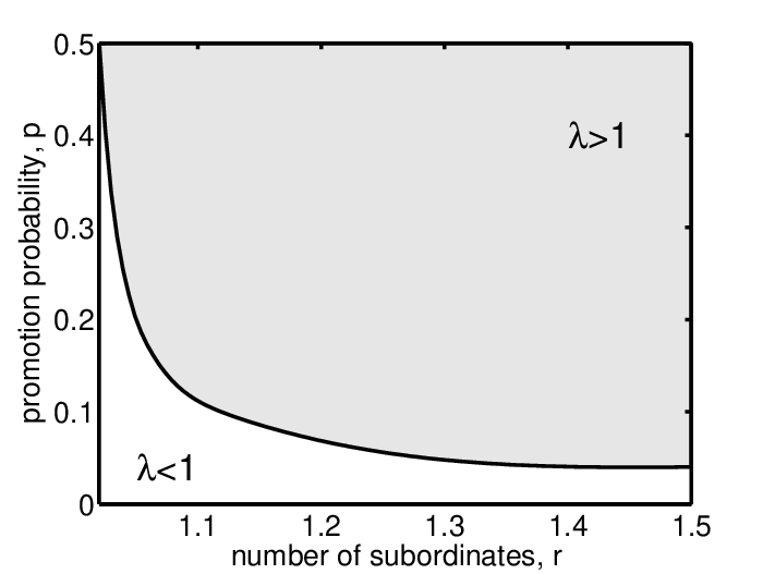
We are finally in the position to answer the century, if not millennium old question how a system of bureaucrats can be organized such that it does not grow exponentially. The phase diagram in Fig. 4 shows the two phases, one of exponential growth, one of shrinking, for administrative bodies evolving according to Parkinson’s Law. The line separating these two phases (given by $\lambda=1$) shows how the parameters $r$ (number of subordinates) and $p$ (average promotion probability) should be adjusted to keep the size of the bureaucracy constant (drop-out rate was set to $\gamma=0.01$).

To fully understand Parkinsonian growth of administrations we now determine the age of retirement $\tau_{R}$. Parkinson suggests that the optimal value for $\tau_{R}$ has to be found on the basis of an administrative body’s promotion scheme. The age of retirement thus does not depend on the actual age of the official whose retirement we are considering, but on his possible successors which should be given the possibility to advance in their careers. If this is not ensured a mechanism nowadays called ’Prince Charles Syndrome’ sets in, i.e. the official gets frustrated by a lack of promotion opportunities, and individual efficiency decreases.

We assume the hierarchical structure of the administrative body to be built according to the motif force that ’Officials try to maximize subordinates, not rivals’, i.e. each official seeks to achieve a number $r$ of subordinates. One can picture this structure as a pyramid consisting of horizontal layers of officials holding an equally high office. On the hierarchical level above there are then $1/r$ times less, on the level below $r$ times more officials. Let us label the levels in the pyramid by an index $l$, then there are $r^{l}$ officials at level $l$. If we fix the number of levels to $L$ we have $N=\sum_{l=0}^{L}r^{l}$ and $l\in\{0,\dots,L\}$. We assign to each official $i$ an efficiency $\epsilon_{i}$ which depends on the years he has served and his current position. We use the career stages given as in Tab. 1, and assign an $\epsilon_{i}$ to each stage, increasing linearly. These career stages are used as a tribute as in [1], but one could equally well work with other efficiency curves. The only important feature is the existence of a bifurcation point reflecting the age where the Prince Charles Syndrome sets in, here this is stage 6. At stage 1 we have $\epsilon_{i}=0.1$. For each subsequent stage (left column) it increases by $0.1$. If after reaching stage 6 the official $i$ reached a promoted position his efficiency proliferates. If at stage 6 we still find him in a subordinate position, his efficiency will decline by $0.1$ in each of the following stages (right column). We introduce the parameter $L^{\prime}$ which is the lowest level which is counted as promoted. The subordinate staff is then present on the levels $L^{\prime}<l\leq L$. The number of subordinate levels is called $\Delta L=L-L^{\prime}$.

We numerically study this system in the following way. It is initialized with randomly distributed ages (and therefore efficiencies) and $r=2$. One time step in the simulation corresponds to one year. At each iteration each official ages by one year and his efficiency is updated according to Tab. 1. If he reaches the age $\tau_{R}$ he retires and his position becomes vacant. One of his two subordinates is chosen randomly to replace him, leaving a vacant position one level below, triggering a cascade of promotions. When the lowest hierarchical level $L$ is reached the vacant position is taken by a new official who enters the system at stage 1. This process is iterated until the average efficiency in the system – $\langle\epsilon_{i}\rangle_{N}$, the mean of $\epsilon_{i}$ over all officials $i=1,\dots,N$ – approaches a stationary value. Simulation results are shown in Fig. 5. We vary $\tau_{R}$ and compute the average efficiency $\langle\epsilon_{i}\rangle_{N}$ for systems of sizes $L=3,\dots,7$ and $\Delta L=$1 (green slash-dotted lines), 2 (red slashed lines), 3 (blue solid lines). For increasing $L$ the system approaches a stationary state where the efficiency only depends on $\Delta L$. Accordingly we find three bundles according to $\Delta L=1,2,3$ with curves for different values of $L$ discernible. Curves of same color and style correspond to increasing $L$ from bottom to top. For each bundle we find a unique maximum indicating the optimal choice for $\tau_{R}$. For values of $\tau_{R}$ below this maximum officials retire too early to reach higher efficiencies, above this point the Prince Charles Syndrome becomes a danger. We further see that the flatter the hierarchy, i.e. higher $\Delta L$, the lower the optimal age of retirement. Recall that we defined the ratio between promoted and subordinate staff as $\mu=\frac{N^{+}\left(t\right)}{N^{-}\left(t\right)}=\frac{\sum_{l=0}^{L-\Delta L-1}r^{l}}{\sum_{l=L-\Delta L}^{L}r^{l}}$. By re-labelling the summation index we can write this as $\left(\sum_{l=0}^{\Delta L}r^{l}\right)^{-1}\sum_{l=1}^{L-\Delta L}\left(\frac{1}{r}\right)^{l}$ which for large $L$ and $r>1$ converges to

$$\mu=\left(\sum_{l=0}^{\Delta L}r^{l}\right)^{-1}\quad.$$

(14)

For large system sizes the ratio $\mu$ indeed approaches a stationary value. So $\Delta L$ determines $\mu$ and the best choice for $\tau_{R}$, which in turn can be used to compute the growth rate $\lambda$ from the previous model.

We quantified three famous, descriptive essays of C.N. Parkinson on bureaucratic inefficiency in a dynamical socio-physical framework. In the first model we showed how the use of recent opinion formation models for small groups could be used to understand Parkinson’s observation – which we showed is still valid in modern data – that decision making bodies such as cabinets or boards become highly inefficient once their size exceeds a critical ’Coefficient of Inefficiency’. We showed how this characteristic size arises due to finite-size effects in the process of forming of coalitions in small systems. Parkinson’s Law states that the growth of bureaucratic or administrative bodies usually goes hand in hand with a drastic decrease of its overall efficiency. In our second model we pictured a bureaucratic body as a system of a flow of workers through an administrative body. Officials enter, become promoted to various internal levels within the system over time, and leave the system after having served for a certain time, they retire. Within the proposed model we showed how to compute the phase diagram under which conditions bureaucratic growth can be confined. We thereby link Parkinson’s microscopic interaction rules to macroscopic properties observable in administration and bureaucracy. It is possible to adjust the ’microscopic’ model parameters – which are altogether observable and measurable –, the individual promotion probability and number of subordinates, to control the growth rate of the bureaucratic body. In our last model we assign individual efficiency curves to workers throughout their life in administration, and compute the optimum time to send them into retirement, in order to ensure a maximum of efficiency within the body, Parkinson’s ’Pension Point’. We implement Parkinson’s observation that an individual’s efficiency declines if he resides in a subordinate position for too long, i.e. the individual efficiency curves over time are characterized by the existence of bifurcation points. This effect necessitates the need of promotion opportunities, which can be ensured by two mechanisms here. On the one hand one can lower the age of retirement allowing young workers to advance in their career faster, or on the other hand one can increase the levels of internal hierarchy.

References

- [1] Parkinson, C.N. Parkinson’s Law and other studies in administration (Buccaneer Books, Cutchogue, 1957).
- [2] Klimek, P., Hanel, R., Thurner, S. e-print: arXiv:0804.2202v1[physics.soc-ph].
- [3] Chiefs of state and cabinet members of foreign governments (Central Intelligence Agency, Washington D.C., 2007).
- [4] Human development report 2007/2008 (United Nations Development Programme, New York, 2007).
- [5] Kaufmann, D., Kraay, A. & Mastruzzi, M. Policy, Research working paper WPS 4280 (2007).
- [6] Liggett, T.J. Stochastic interacting systems: contact, voter and exclusion processes (Springer Verlag, New York, 1999).
- [7] Asch, S.E. Social psychology (Englewood Cliffs, Prentice Hall, New Jersey, 1952).
- [8] Kelman, H. J. Conflict Resolut. 2, 51-60 (1958).
- [9] Watts, D.J. Small worlds (Princeton University Press, Princeton, NJ, 1997).
- [10] Ben-Naim, E., Frachebourg, L. & Krapivsky, P.L. Phys. Rev. E 53, 3078 (1996).
- [11] Axelrod, R. J. Conflict Resolut. 41, 203 (1997).
- [12] Krapivsky, P.L. & Redner, S. Phys. Rev. Lett. 90, 238701 (2003).
- [13] Castellano, C., Loretto, V., Barrat, A., Cecconi, F. & Parisi, D. Phys. Rev. E 71, 066107 (2005).
- [14] Watts, D.J. Proc. Nat. Acad. Sci. 99, 5766-5771 (2002).
- [15] Klimek, P. Lambiotte, R. & Thurner, S. Europhys. Lett., 82, 2, 28008 (2008).