Decoding the Mechanism for the Origin of Dark Matter
in the Early Universe Using LHC Data

Introduction. In the near future, data from the LHC will be available allowing one to test models of physics beyond the Standard Model (SM). Supersymmetry (SUSY) and more specifically supergravity grand unified models[1, 2, 3] provide a well motivated framework for the exploration of new physics. Thus supergravity grand unified models naturally lead to the lightest neutralino as the lightest SUSY particle, or the LSP, over a significant part of the parameter space and with R parity it is then a candidate for dark matter. An analysis of the relic density of the LSP reveals three broad regions where the WMAP [4] constraints are satisfied: these include (1) the Hyperbolic Branch (HB)[5, 6] where multi TeV scalars can appear consistent with small fine tuning (this region is alternately referred sometimes as the Focus Point region (FP) or as HB/FP), (2) the coannihilation regions[7, 8, 9, 10, 11], (3) the Higgs pole region[12] (for recent work on these regions(1-3) see [13, 14, 15, 16]). Of these, the stau coannihilation region and the HB region are more generic while the pole region (light Higgs and the CP odd Higgs $A$) is more fine tuned. In addition there is also the parameter space in the bulk region where the relic density is satisfied due to a combination of effects. An interesting issue relates to the following: to what extent the LHC data will allow one to decode the mechanism by which dark matter is generated in the early universe. Specifically we will focus on dark matter originating in the Stau-Co region or in the HB region to answer this question.

For concreteness we work within the framework of the mSUGRA model[1], which is characterized by the parameters $m_{0},m_{1/2},A_{0},\tan\beta$ and sign$(\mu)$, where $m_{0}$ is the universal scalar mass, $m_{1/2}$ is the universal gaugino mass, $A_{0}$ is the universal trilinear coupling (all at the grand unification scale), and $\tan\beta\equiv\langle H_{2}\rangle/\langle H_{1}\rangle$ where $H_{2}$ gives mass to the up quarks and $H_{1}$ gives mass to the down quarks and the leptons, while $\mu$ is the Higgs mixing parameter. The parameter space of mSUGRA investigated in this work is as in [14]. In this framework we will show that the LHC signatures carry sufficient information for the discrimination between the Stau-Co and the HB regions.

In the analysis, the sparticle masses and mixings are derived from the GUT scale with the SuSpect code [17] coupled to micrOMEGAs [18]. We merge the models via the SUSY Les Houches Accord format [19] into Pythia [20] for the computation of SUSY production at the LHC, in concert with PGS4 [21], to simulate LHC detector effects, and obtain the final event record. The models are constrained by their ability to properly break electro-weak symmety, by sparticle mass limits from LEP and Tevatron analyses, FCNC constraints including $b\to s\gamma$ and $B_{s}\to\mu^{+}\mu^{-}$, by the supersymmetric contribution to the muon anomalous magnetic moment, and the double sided bound on the relic density (see [22, 16] for details). Our post trigger level cuts are as given in [16] and are standard and we list them below: (1) In an event, we only select photons, electrons, and muons that have transverse momentum $P_{T}(p)>10$ GeV and $|\eta(p)|<2.4$, $p=(\gamma,e,\mu)$; (2) For hadronically decaying tau (jets): $P_{T}(\tau)>10$ GeV and $|\eta(\tau)|<2.0$ are selected; (3) For other hadronic jets only those satisfying $P_{T}(jet)>60$ GeV and $|\eta(jet)|<3.0$ are selected; (4) We require a large amount of missing transverse momentum, $P^{miss}_{T}>200$ GeV; (5) There are at least two jets that satisfy the $P_{T}$ and $\eta$ cuts. Variations on (4) and (5) will be discussed later.

The SM background was determined through the generation of events from QCD multi-jets from light and heavy quark flavors, Drell-Yan, single $Z/W$ production along with quarks and gluons ($Z$/$W$ + jets), and $ZZ$, $WZ$, $WW$ pair production which give multi-lepton backgrounds. We have cross checked our SM backgrounds and several other elements of our analysis with simulations done by CMS [23, 24] and the results of these checks are in good agreement. We have also found good agreement with the SUSY signal analyses of [23, 24] and the total background analysis of [15] under similar cuts. In PGS4 jets are defined through a cluster-based algorithm which has a heavy flavor tagging efficiency based on the parameterizations of the CDF Run 2 tight/loose SECVTX tagger [25] and is a displaced (secondary) vertex b-tagging algorithm which allows detection of b quarks. The b-tagging efficiency enters as a product of two polynomials each a separate function of $|\eta(jet)|$ and $P_{T}(jet)$. The efficiency is maximized in the region $|\eta(jet)|<1$ with maximal efficiency ${\epsilon}_{b}=(0.4,0.5)$ for tight and loose tags respectively, and falls off sharply for $|\eta(jet)|>1$ with virtually zero efficiency out near $|\eta(jet)|=2$ and $P_{T}(jet)\sim 160$ GeV. The analysis of tau decays is done using Tauola[26](For further details regarding PGS4 see [27]).

There are several recent works which discuss dark matter[28, 29, 30, 31, 36, 32, 33, 34, 35] and collider physics [37, 38, 39, 40, 41, 42, 43, 44, 45, 46, 47]. The analysis presented here is very focused in that it connects LHC signatures directly to the possible origin of dark matter, and here we consider two dominant mechanisms, i.e., stau coannihilation and annihilation on the HB. We do not go into the details of the relic density analysis which are standard. Rather we go directly to a discussion of how the experimental data, in particular the LHC data, can allow one to decode the mechanism for the generation of dark matter.

Decoding the mechanism for the generation of dark matter with LHC data: It is well known that in the stau coannihilation region, the neutralino is typically Bino like while in the HB region there is a significant Higgsino component. In the analysis of [14] it was shown that the Stau-Co region is constituted of a collection of mass hierarchical patterns, where mSP5 is the dominant pattern (defined by the mass hierarchy: $\widetilde{\chi}^{0}_{1}$ $<$ $\widetilde{\tau}_{1}$ $<$ $\widetilde{l}_{R}$ $<$ $\widetilde{\nu}_{\tau}$). Similarly the analysis of [14] shows that the HB region is dominated by the chargino patterns, where the chargino $\tilde{\chi}_{1}^{\pm}$ is the NLSP, and were classified in [14] as mSP1-mSP4 (where mSP1 is the dominant pattern defined by the mass hierarchy: $\widetilde{\chi}^{0}_{1}$ $<$ $\widetilde{\chi}^{\pm}_{1}$ $<$ $\widetilde{\chi}^{0}_{2}$ $<$ $\widetilde{\chi}^{0}_{3}$). The largest cross sections in the direct detection experiments arise from a Chargino Wall (CW) [31] constituted uniquely of mSP1. Along the Wall the thermal annihilation cross sections in the early universe would have arisen mostly from $\widetilde{\chi}^{0}_{1}\widetilde{\chi}^{0}_{1}$ annihilations into $WW,ZZ,t\bar{t},b\bar{b}$ for the Higgsino like LSP. Additionally there are a significant number of cases where the annihilation is dominated by the processes $\widetilde{\chi}^{0}_{1}\widetilde{\chi}^{0}_{1}\to b\bar{b}~[\sim(85-90)\%]$ and $\widetilde{\chi}^{0}_{1}\widetilde{\chi}^{0}_{1}\to\tau^{+}\tau^{-}~[\sim(5-10)\%]$, and these cases typically occur for larger neutralino masses which are more Bino like, but can also occur for low values of the neutralino masses as well on the CW.

The Chargino Wall referred to above enters importantly in the analysis of LHC signatures. It refers to the region of HB where the NLSP is the lightest chargino, the LSP is mostly higgsino like, and the spin independent cross section is essentially constant $O(10^{-8})$ pb as function of the neutralino mass for neutralino mass in the range $\sim$(80-650) GeV. To explain this feature we begin by exhibiting the LSP $\tilde{\chi}_{1}^{0}$ state in terms of the gaugino-Higgsino states so that $\widetilde{\chi}^{0}_{1}\equiv\chi=n_{1}{\tilde{B}}+n_{2}{\tilde{W}}^{3}+n_{3}{\tilde{H}}^{0}_{1}+n_{4}{\tilde{H}}^{0}_{2}.$ The LSP gaugino-Higgsino content enters importantly in the thermal annihilation cross sections that determine the proper relic density of decoupled neutralinos from the epoch of freeze out. It also enters prominently in the strength of the scalar neutralino-proton cross section which we now discuss. Thus on the Wall the heavier of the CP Higgs mass has a lower limit near 300 GeV and more typically it extends into the range of a TeV to several TeV. On the CW one typically has $m^{2}_{H}\gg m^{2}_{h}$, and $\sin\alpha\approx\alpha$ where $\alpha$ is the Higgs mixing parameter which enters in the diagonalization of the CP even Higgs mass² matrix. Further, the sfermion poles can be neglected as they make a small contribution in this region. Under the above limits one finds that the product $\alpha\times\tan\beta$ is essentially a constant, i.e., $\alpha\times\tan\beta\simeq-1$. Under this circumstance the spin independent cross section in the absence of CP phases is given by [48, 49, 50]

Here $\mu_{\chi p}$ is the reduced mass, and $f_{p}$ and $f_{pG}$ are matrix elements defined by $f_{p}=\sum_{i=u,d,s}f_{i}^{p}$, $f_{pG}=(1-f_{p})$ where $m_{p}f_{i}^{(p)}=\langle p|m_{q_{i}}\bar{q}_{i}q_{i}|p\rangle$. The typical ranges for $n_{i}$ on the wall are: $n_{1}\in(.85,.99)$, $n_{2}\ll n_{1}$, and $n_{3}\in(.1,.6)\sim-{\cal O}(n_{4})$. Using numerical values of $f_{p},f_{pG}$[48, 49, 50] one gets $\sigma^{\rm SI}_{\chi p}({\rm WALL})\sim 2\times 10^{-8}$[pb]. In our analysis presented later (see Fig.(5)), however, we have implemented the full cross section calculation without any of the above approximations. This analysis leads to $\sigma^{\rm SI}_{\chi p}$ $({\rm WALL})$ lying in the range $\sim(1.5-5)\times 10^{-8}$ pb while the most recent limits give $\sigma^{\rm SI}_{\chi p}\sim 5\times 10^{-8}$ pb[51] for $m_{\chi}\approx 60$ GeV. Thus this region of the parameter space is within reach of the current and the next generation of dark matter experiments. As noted already, the CW is also a very interesting region for LHC signatures. In the following we discuss several signatures [listed as (i)-(v)] which allow one to discriminate between the Stau-Co and the HB regions over a significant part of the parameter space.

(i) $P_{T}^{\rm miss}$Distributions: A powerful signature for the discrimination of Stau-Co and HB is the total number of SUSY events $N_{\rm SUSY}$ as a function of the missing transverse momentum. An analysis of this signature is given in Fig.(1) (left panel) where one finds different geometries in these distributions. Here we emphasize that the significantly fatter $P_{T}^{\rm miss}$distributions for points in the Stau-Co region contrast sharply with the $P_{T}^{\rm miss}$distributions from points in the HB region which are much thinner[16] as exhibited for the case given in Fig.(1)(left panel). Such a signature has the interesting feature in that the discovery potential is increased over a larger region in the SUGRA parameter space than for the case of counting fractional number of such events in separate channels. The above is due in part because every SUSY event that passes the trigger has $P^{\rm miss}_{T}$, and so one maximizes the signal events as opposed to obtaining a fraction of them. Further, the SM $P^{\rm miss}_{T}$ falls off rapidly beyond the peak value coupled with the fact the $P^{\rm miss}_{T}$ is larger in SUSY extending out to momenta where the SM cannot produce a large number of events.
(ii) $\langle P_{T}^{\rm miss}\rangle$ Analysis: A remarkable signature emerges distinguishing the stau coannihilation region and the HB region if one analyzes $N_{\rm SUSY}$ for each parameter point as a function of $\langle P_{T}^{\rm miss}\rangle$ which is the mean $P_{T}^{\rm miss}$ calculated by averaging the $P_{T}^{\rm miss}$ over the entire model event record. The above phenomenon is shown in Fig.(1) (right panel). Here one finds that $\langle P_{T}^{\rm miss}\rangle$ has a very wide range from 300 GeV to a TeV or more for the stau coannihilation region, while $\langle P_{T}^{\rm miss}\rangle$  for the HB region lies in a much narrower band centered around 350 GeV - a phenomenon which originates for parameter points on the Chargino Wall. Thus the $\langle P_{T}^{\rm miss}\rangle$ ranges in Fig.(1)(right panel) can be viewed as one of the smoking gun signatures which can discriminate between the two mechanisms using LHC data.

Although a quantitative analysis of $\langle P_{T}^{\rm miss}\rangle$ is rather complicated since it involves many particles and depends in part on post trigger level cuts, one can give a qualitative picture of the disparity between the $P_{T}^{\rm miss}$ on the Stau-Co and the HB regions by analyzing the decay chains of sparticles into their final products culminating into an odd number of LSPs (per sparticle decay chain) and the SM particles. Here one finds that often the sparticle decays on the Stau-Co involve two body decays. For the HB case, however, one finds that the sparticles produced in $pp$ collisions have typically a longer decay chain which depletes the $P_{T}^{\rm miss}$ in this case.

We illustrate these features by analyzing the two specific benchmarks given in the caption of Fig.(1)(left panel). For the HB model point of Fig.(1)(left panel) the following production cross sections are dominant: $pp\to(\widetilde{g}\widetilde{g}/\widetilde{\chi}^{0}_{2}\widetilde{\chi}^{\pm}_{1}/{\widetilde{\chi}^{\pm}_{1}}{\widetilde{\chi}^{\mp}_{1}}$) at the level of $(45,25,15)\%$. While squark production is highly suppressed ($m_{\widetilde{g}}\sim 622~{\rm GeV}\ll m_{\widetilde{q}_{L},\widetilde{q}_{R},\widetilde{b}_{1},\widetilde{t}_{1}}\in(1.2,1.7)~{\rm TeV}$). One finds that the dominantly produced $\tilde{g}$ decays via ${\rm Br}[\widetilde{g}\to{\widetilde{\chi}}^{0}_{i}+q+\bar{q}]\sim 50\%$ and ${\rm Br}[\widetilde{g}\to{\widetilde{\chi}}^{\pm}_{j}+q+\bar{q}^{\prime}]\sim 50\%$ with the LSP contributing only $10\%$. The reason for this largeness is because the on-shell decay of the gluino into $q\tilde{q}$ is suppressed due to largeness of the squark masses (a phenomenon which typically holds for the gluino decays on the HB). Further, the $\widetilde{\chi}^{0}_{2}$ and $\widetilde{\chi}^{\pm}_{1}$ produced on HB have ${\rm Br}[\widetilde{\chi}^{0}_{2}\to{\widetilde{\chi}}^{0}_{1}+f+\bar{f}]\sim 100\%$ and ${\rm Br}[{\widetilde{\chi}_{1}}^{\pm}\to{\widetilde{\chi}^{0}_{1}}+f+\bar{f}^{\prime}]\sim 100\%$. Thus the decay chain for sparticles produced on the HB tend to be longer resulting in reduced $P_{T}^{miss}$ Now, for the Stau-Co model point of Fig.(1)(left panel) the leading SUSY production level cross sections are from $(\widetilde{g}{\widetilde{q}},{\widetilde{q}}{\widetilde{q}},\widetilde{g}\widetilde{g})$ at the level of $(41,33,7)\%$, with the corresponding 2 body decay modes ${\rm Br}[\widetilde{q}_{R}\to\widetilde{\chi}^{0}_{1}+q]\sim 100\%$ (1st and 2nd generation), and ${\rm Br}[\widetilde{q}_{L}\to(\widetilde{\chi}^{0}_{2},\widetilde{\chi}^{\pm}_{1})+(q,q^{\prime})]\sim(60,30)\%$. Since the decay chain for sparticles on the Stau-Co tend to be shorter the resulting $P_{T}^{miss}$ is larger. In summary the main reason why the HB tends to give lower values of missing $P_{T}$ relative the Stau-Co is simply due to the fact that on the HB, in order to get to the LSP from the dominant gluino production mechanism one usually needs at least 2 successive 3 body decays, while on the Stau-Co the right-squarks ($\tilde{q}_{R}$) from the first and second generations, which are dominantly produced, each decays right into the LSP + quark. The above also holds more generally in that one finds that sparticles arising from the Stau-Co have much shorter decay chains resulting in fewer final particles and thus the missing energy can get large. Our more general results given here on a large spread in $P^{\rm miss}_{T}$ agree with the first Ref. of [13] and with the analyses of the CMS and ATLAS collaborations [53, 54, 55]. Conversely the models on the HB have longer decay chains with more final state particles and thus the missing energy carried by the neutrals is depleted leading to missing $P_{T}^{\rm miss}$ which is more SM like. This feature has also been discussed in the CMS analysis of [56].

(iii) Jet cuts, $n_{jet}^{*}$: Another powerful signature for discriminating the Stau-Co and the HB regions is $N_{\rm SUSY}$ taken as a function of $P_{T}^{\rm*miss}$and $n_{jet}^{*}$, i.e.,

where the $*$ indicates a fixed cut value. Here features specific to the coannihilation branch and to the HB emerge when $P^{*\rm miss}_{T}$ is fixed, and $n_{jet}^{*}$  is varied. This is shown in Fig.(2). In particular one finds that for the coannihilation branch there is an optimal $n_{jet}^{*}$ near 4 because the discovery limit criteria $N^{\rm Stau-Co}_{\rm SUSY}/\sqrt{{\rm SM}}$ decreases as a function of increasing $n_{jet}^{*}$ and has a max near $n_{jet}$ $\sim$ 4, while for the annihilations on the HB, specifically on the Wall, the situation is quite different, in that the larger the $n_{jet}^{*}$ the larger is the value of $N^{\rm HB}_{\rm SUSY}/\sqrt{{\rm SM}}$ (where of course the SM is subject to the same * cuts). Thus, as the jet number $n_{jet}^{*}$ becomes large $N^{\rm HB}_{\rm SUSY}$ sustains a much stronger signal than $N^{\rm Stau-Co}_{\rm SUSY}$, and thus $N_{\rm SUSY}/\sqrt{\rm SM}$ is a strong discriminator between the Stau-Co and the HB regions.

The above becomes very significant if the SUSY scale is high with the LSP mass lying in the several hundred GeV range. Also, this type of large n-jet cut can deplete the leptonic signal, so a delicate balance of jet cuts is very important. In fact, if the SUSY signal is not highly leptonic, the analysis of the above type would be an efficient way to decipher new physics. Further, even if one has signatures with many leptons, the jet analysis will provide additional corroborating signatures for discovery and discrimination.

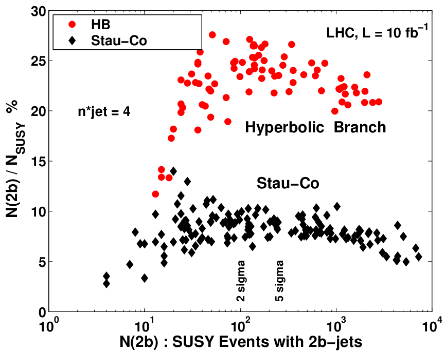
(iv) Tagged b-jets: The utility of b-tagging for the HB region has previously been emphasized in [42, 15, 16]. In Fig. (3)(upper panels) we give an analysis exhibiting how b-tagging provides a striking discrimination between the Stau-Co and HB regions where we plot $N(nb)/\sqrt{{\rm SM}(nb)}$ as a function of the number of tagged b-jets ($nb$) and find this dependence to be drastically different for Stau-Co vs HB regions. In Fig. (3)(lower panel) the fractional number of events with 2b-jets vs the number of events with 2b-jets is given, and again one sees a strong discrimination between the parameter points in the Stau-Co region vs those in the HB region. In Fig.(4) we extend the analysis to the 4b-jet mode and correlate this signature to events with two hadronically decaying tau jets and to events that do not contain tagged b-jets.

As already discussed in (ii), on the HB gluino production is dominant in $pp$ collisions at the LHC, and further one finds that the gluino decays dominantly into $b\bar{b}$, i.e., ${\rm Br}[\widetilde{g}\to{\widetilde{\chi}}^{0}_{i}+b+\bar{b}]\sim 40\%$ and ${\rm Br}[\widetilde{g}\to{\widetilde{\chi}}^{\pm}_{j}+b(\bar{b})+\bar{t}(t)]\sim 40\%$. Thus, the gluino 3 body decays are very rich in b quarks. Conversely for the Stau-Co model point of Fig.(1) (left panel) the $pp$ production cross sections are as follows: $(\tilde{g}\tilde{q})\sim 41\%$, $(\tilde{q}\tilde{q})\sim 33\%$, $(\tilde{g}\tilde{g})\sim 7\%$ (as already noted in (ii)). Further, the gluino has only a small branching ratio into $b\bar{b}$ in this case via $\tilde{g}\to\tilde{b}b$. Including the production cross sections for $\tilde{g}\tilde{g}$ and the branching ratios, we find that overall the $b\bar{b}$ production on Stau-Co is smaller relative to that on the HB. More generally the analysis of Figs.[(1)-(4)] shows that the LHC signatures arising from the Stau-Co are easily distinguishable from those arising from the HB.

(v) $N_{\rm SUSY}(leptons/jets)~{\rm and}~\langle P_{T}^{miss}\rangle~{\rm vs}~\sigma^{\rm SI}_{\chi p}$: Significant additional information regarding the coannihilation region and the HB region can be obtained by an analysis of the number of SUSY events at the LHC vs the spin-independent neutralino-proton cross section $\sigma^{\rm SI}_{\chi p}$ along with the current limits from the direct detection of dark matter. We give an illustration of the above in Fig.(5). The analysis of Fig.(5) (right panel) shows that the coannihilation and the HB regions are well separated in the space spanned by the trileptonic signature 3L (L=$e$,$\mu$) and $\sigma^{\rm SI}_{\chi p}$. Further one observes that in Fig.(5) (left panel) the parameter points in the HB region in the $\langle P^{miss}_{T}\rangle-\sigma^{\rm SI}_{\chi p}$ plot are clustered together in a ball shaped region and well separated from points in the Stau-Co region which lie on a slope again providing a strong discrimination between the Stau-Co and the HB regions.

In the above we have analyzed in detail how the LHC data can allow one to discover if the mechanism for the origin of dark matter in the early universe arises in the HB region or in the Stau-Co region. This opens up the issue if the above type analysis can be done more generally to identify the dominant mechanism for the generation of dark matter in the early universe using LHC data. Below we discuss briefly how one may extend the analysis to the stop coannihilation region and the A-pole region. Thus as already discussed in the introduction, in addition to the Stau-Co region there is also a stop coannihilation (Stop-Co) region where the relic density constraint is satisfied. However, regions of the parameter space which give rise to Stop-Co have signatures which are highly non-leptonic relative to those of the Stau-Co and of the HB [14, 16]. Thus correlations such as 0L + jets vs 1L+ jets allow one to distinguish Stop-Co regions from others as discussed in the analysis of [14, 16]. Such correlations if observed, would be a good indication of stop coannihilation as the origin of dark matter. We note in passing that the LSP is mostly a Bino in this case which suppresses the scalar cross sections in the direct detection of dark matter[31]. Next we discuss the $A$-funnel region. Here the relic density is satisfied because the LSP mass is nearly half the CP odd Higgs mass. The analysis of parameter points which cluster near the pole region do not have the same NLSP for all parameter points unlike the case of HB where $\tilde{\chi}_{1}^{\pm}$ is the NLSP, or the Stau-Co region where $\tilde{\tau}_{1}$ is the NLSP. However, in the pole region the NLSP could be $\tilde{\chi}_{1}^{\pm}$ or $\tilde{\tau}_{1}$ ($\tilde{t}_{1}$ is seldom seen in the pole region). Thus the $A$-pole region can give mixed signatures, sometimes characteristic of HB and sometimes characteristic of the Stau-Co. To firmly establish the pole region one would need a global analysis with many signatures which would give a determination of the Higgs $A^{0}$ mass and the mass of the LSP. A similar situation holds for other isolated regions of the parameter space which cannot be classified in the above categories which satisfy the relic density constraints. Here also one would need a global analysis on the signatures to identify the mechanism regarding the origin of dark matter.

Conclusions: The analysis presented here shows that with sufficient LHC data one can discriminate between the Stau-Co and the HB regions regarding the origin of dark matter in the early universe in the mSUGRA model using lepton, jet and missing energy signatures. We discussed several smoking gun signatures for such a discrimination. It was also shown that further discrimination is possible by combining LHC data with the limits on $\sigma^{\rm SI}_{\chi p}$ from the direct detection of dark matter. An analysis in a similar spirit is given in [39]. Our analysis utilizes simulations based on CMS detector specifications and specific final state signatures in probing the origin of dark matter, and we do so over a large portion of the parameter space. To our knowledge there are no analyses in the literature which have tried to utilize the expected LHC signatures to probe the origin of dark matter along the lines discussed here. While the analysis presented in our work illustrates our main points in the mSUGRA model, similar analyses along these lines should be pursued for other models of soft breaking including string and D brane models. Specifically, it would be interesting to analyze what the LHC can tell us about the origin of dark matter in cases where one has departures from mSUGRA including the case of a non-thermal relic such as a Wino dominated neutralino.

Acknowledgements: This work is supported in part by the U.S. NSF grant PHY-075959.

References

- [1] A. H. Chamseddine, R. Arnowitt and P. Nath, Phys. Rev. Lett. 49 (1982) 970.
- [2] L. Hall, J. Lykken and S. Weinberg, Phys. Rev. D27, 2359 (1983); P. Nath, R. Arnowitt and A. H. Chamseddine, Nucl. Phys. B 227, 121 (1983).
- [3] For a review see, P. Nath, R. Arnowitt and A.H. Chamseddine, ”Applied N=1 supergravity”, (World Scientific, Singapore,1984); H. P. Nilles, Phys. Rept. 110, 1 (1984); P. Nath, arXiv:hep-ph/0307123.
- [4] D. N. Spergel et al. Astrophys. J. Suppl. 170, 377 (2007).
- [5] K. L. Chan, U. Chattopadhyay and P. Nath, Phys. Rev. D 58, 096004 (1998); J. L. Feng, K. T. Matchev and T. Moroi, Phys. Rev. Lett. 84, 2322 (2000); H. Baer, C. Balazs, A. Belyaev, T. Krupovnickas and X. Tata, JHEP 0306, 054 (2003). For a review see, A. B. Lahanas, N. E. Mavromatos and D. V. Nanopoulos, Int. J. Mod. Phys. D 12, 1529 (2003).
- [6] U. Chattopadhyay, A. Corsetti and P. Nath, Phys. Rev. D 68, 035005 (2003).
- [7] K. Griest and D. Seckel, Phys. Rev. D 43, 3191 (1991).
- [8] M. Drees and M. M. Nojiri, Phys. Rev. D 47, 376 (1993).
- [9] S. Mizuta and M. Yamaguchi, Phys. Lett. B 298, 120 (1993).
- [10] J. Edsjo and P. Gondolo, Phys. Rev. D 56, 1879 (1997); J. R. Ellis, T. Falk and K. A. Olive, Phys. Lett. B 444 (1998) 367; J. R. Ellis, T. Falk, K. A. Olive and M. Srednicki, Astropart. Phys. 13, 181 (2000).
- [11] T. Nihei, L. Roszkowski and R. Ruiz de Austri, JHEP 0207, 024 (2002).
- [12] P. Nath and R. L. Arnowitt, Phys. Rev. Lett. 70, 3696 (1993); Phys. Lett. B 299, 58 (1993) [Erratum-ibid. B 307, 403 (1993)]; J. L. Lopez, D. V. Nanopoulos and K. j. Yuan, Phys. Rev. D 48, 2766 (1993); H. Baer and M. Brhlik, Phys. Rev. D 53, 597 (1996); V. D. Barger and C. Kao, Phys. Rev. D 57, 3131 (1998).
- [13] R. L. Arnowitt, B. Dutta, T. Kamon, N. Kolev and D. A. Toback, Phys. Lett. B 639, 46 (2006); R. Arnowitt, B. Dutta, A. Gurrola, T. Kamon, A. Krislock and D. Toback, arXiv:0802.2968 [hep-ph]
- [14] D. Feldman, Z. Liu and P. Nath, Phys. Rev. Lett. 99, 251802 (2007).
- [15] H. Baer, V. Barger, G. Shaughnessy, H. Summy and L. t. Wang, Phys. Rev. D 75, 095010 (2007).
- [16] D. Feldman, Z. Liu and P. Nath, JHEP 0804, 054 (2008) [arXiv:0802.4085 [hep-ph]]; arXiv:0806.4683 [hep-ph].
- [17] A. Djouadi, J. L. Kneur and G. Moultaka, Comput. Phys. Commun. 176, 426 (2007).
- [18] G. Belanger, F. Boudjema, A. Pukhov and A. Semenov, Comput. Phys. Commun. 177, 894 (2007); arXiv:0803.2360 [hep-ph].
- [19] P. Skands et al., JHEP 0407, 036 (2004).
- [20] T. Sjostrand, S. Mrenna and P. Skands, JHEP 0605, 026 (2006).
- [21] PGS4, J. Conway et al.
- [22] A. Djouadi, M. Drees and J. L. Kneur, JHEP 0603, 033 (2006).
- [23] M. Chiorboli, M. Galanti, A. Tricomi, CERN-CMS-NOTE-2006-133; D. J. Mangeol, U. Goerlach, CERN-CMS-NOTE-2006-096.
- [24] W. de Boer et. al, CERN-CMS-NOTE-2006-113.
- [25] D. E. Acosta et al. [CDF Collaboration], Phys. Rev. D 71, 052003 (2005).
- [26] S. Jadach, Z. Was, R. Decker and J. H. Kuhn, Comput. Phys. Commun. 76, 361 (1993).
- [27] http://v1.jthaler.net/olympicswiki/doku.php
- [28] A. Djouadi, M. Drees and J. L. Kneur, Phys. Lett. B 624, 60 (2005).
- [29] L. Roszkowski, R. Ruiz de Austri and R. Trotta, JHEP 0707 (2007) 075; R. R. de Austri, R. Trotta and L. Roszkowski, JHEP 0605, 002 (2006).
- [30] B. C. Allanach, K. Cranmer, C. G. Lester and A. M. Weber, JHEP 0708, 023 (2007); B. C. Allanach, C. G. Lester and A. M. Weber, JHEP 0612, 065 (2006); F. Feroz, B. C. Allanach, M. Hobson, S. S. AbdusSalam, R. Trotta and A. M. Weber, arXiv:0807.4512 [hep-ph].
- [31] D. Feldman, Z. Liu and P. Nath, Phys. Lett. B 662, 190 (2008) [arXiv:0711.4591 [hep-ph]].
- [32] A. Belyaev, S. Dar, I. Gogoladze, A. Mustafayev and Q. Shafi, arXiv:0712.1049 [hep-ph].
- [33] G. Barenboim, P. Paradisi, O. Vives, E. Lunghi and W. Porod, JHEP 0804, 079 (2008).
- [34] B. C. Allanach and D. Hooper, arXiv:0806.1923 [hep-ph].
- [35] V. Barger, W. Y. Keung and G. Shaughnessy, arXiv:0806.1962 [hep-ph].
- [36] J. L. Kneur and N. Sahoury, arXiv:0808.0144 [hep-ph].
- [37] B. C. Allanach, G. A. Blair, S. Kraml, H. U. Martyn, G. Polesello, W. Porod and P. M. Zerwas, arXiv:hep-ph/0403133.
- [38] M. M. Nojiri, G. Polesello and D. R. Tovey, JHEP 0603, 063 (2006).
- [39] E. A. Baltz, M. Battaglia, M. E. Peskin and T. Wizansky, Phys. Rev. D 74, 103521 (2006).
- [40] M. S. Carena, D. Hooper and P. Skands, Phys. Rev. Lett. 97, 051801 (2006).
- [41] H. Baer and X. Tata, arXiv:0805.1905 [hep-ph].
- [42] H. Baer, C. h. Chen, F. Paige and X. Tata, Phys. Rev. D 52, 2746 (1995); U. Chattopadhyay, A. Datta, A. Datta, A. Datta and D. P. Roy, Phys. Lett. B 493, 127 (2000); P. G. Mercadante, J. K. Mizukoshi and X. Tata, Phys. Rev. D 72, 035009 (2005); R. H. K. Kadala, P. G. Mercadante, J. K. Mizukoshi and X. Tata, arXiv:0803.0001 [hep-ph].
- [43] U. Chattopadhyay, D. Das, A. Datta and S. Poddar, Phys. Rev. D 76, 055008 (2007).
- [44] S. P. Martin, Phys. Rev. D 75, 115005 (2007); Phys. Rev. D 76, 095005 (2007); [arXiv:hep-ph/0703097]; arXiv:0807.2820 [hep-ph].
- [45] B. Altunkaynak, M. Holmes and B. D. Nelson, arXiv:0804.2899 [hep-ph].
- [46] G. Kane and S. Watson, arXiv:0807.2244 [hep-ph].
- [47] N. Bhattacharyya, A. Datta and S. Poddar, arXiv:0807.0278 [hep-ph]; N. Bhattacharyya, A. Datta and M. Maity, arXiv:0807.0994 [hep-ph].
- [48] U. Chattopadhyay, T. Ibrahim and P. Nath, Phys. Rev. D 60, 063505 (1999) [arXiv:hep-ph/9811362]; A. Corsetti and P. Nath, Phys. Rev. D 64, 125010 (2001).
- [49] J. R. Ellis, A. Ferstl and K. A. Olive, Phys. Lett. B 481, 304 (2000).
- [50] J. Ellis, K. A. Olive and C. Savage, Phys. Rev. D 77, 065026 (2008).
- [51] Z. Ahmed et al. [CDMS Collaboration], arXiv:0802.3530 [astro-ph]; J. Angle et al. [XENON Collaboration], Phys. Rev. Lett. 100, 021303 (2008).
- [52] R. W. Schnee et al. [The SuperCDMS Collaboration], arXiv:astro-ph/0502435.
- [53] T. Yetkin and M. Spiropulu [CMS Collaboration], Acta Phys. Polon. B 38 (2007) 661.
- [54] M. Biglietti et al., CERN-ATL-PHYS-PUB-2007-004; ATL-COM-PHYS-2006-095;ATL-PHYS-CONF-2007-020; ATL-COM-PHYS-2007-078.
- [55] A. Migliaccio [ATLAS Collaboration], Diploma Thesis.
- [56] B. Mura [CMS Collaboration], Diploma Thesis.