Department of Electrical Engineering and Computer Science \degreeMaster of Engineering in Electrical Engineering and Computer Science \degreemonthJune \degreeyear2008 \thesisdateMay 20, 2008 \supervisorIsaac L. ChuangAssociate Professor
Arthur C. SmithChairman, Department Committee on Graduate Theses
The Study of Entangled States in Quantum Computation and Quantum Information Science
This thesis explores the use of entangled states in quantum computation and quantum information science. Entanglement, a quantum phenomenon with no classical counterpart, has been identified as an important and quantifiable resource in many areas of theoretical quantum information science, including quantum error correction, quantum cryptography, and quantum algorithms.
We first investigate the equivalence classes of a particular class of entangled states (known as graph states due to their association with mathematical graphs) under local operations. We prove that for graph states corresponding to graphs with neither cycles of length 3 nor 4, the equivalence classes can be characterized in a very simple way. We also present software for analyzing and manipulating graph states.
We then study quantum error-correcting codes whose codewords are highly entangled states. An important area of investigation concerning QECCs is to determine which resources are necessary in order to carry out any computation on the code to an arbitrary degree of accuracy, while simultaneously maintaining a high degree of resistance to noise. We prove that transversal gates, which are designed to prevent the propagation of errors through a system, are insufficient to achieve universal computation on almost all QECCs.
Finally, we study the problem of creating efficient quantum circuits for creating entangling measurements. Entangling measurements can be used to harness the apparent extra computing power of quantum systems by allowing us to extract information about the global, collective properties of a quantum state using local measurements. We construct explicit quantum circuits that create entangling measurements, and show that these circuits scale polynomially in the input parameters.
Acknowledgments
I would like to thank Professor Isaac Chuang for accepting me into his research group, and for giving me the opportunity to carry out my MEng thesis project under his supervision. I am grateful for his efforts to help me become a better scientist, by teaching me how to approach research questions, and reminding me to think about the motivation behind every problem, and the consequences of finding a solution. I would also like to thank Professor Chuang for helping to improve my communication skills, in the day-to-day environment of the research group as well as in giving presentations and writing papers.
I would also like to thank all the members of the Quanta group for their insights, conversations, and jokes during our weekly group meetings and other get-togethers, and for answering my questions about their research and my own. I am also grateful to Dave Bacon for patiently answering my questions about his papers, both in person and via e-mail.
Finally, I would like to thank my parents for their unfailing love, encouragement, and support.
Chapter 1 Introduction
The field of theoretical quantum computing and quantum information science has seen an enormous rate of growth in the past two or three decades [NC04, HDE+06, Pre98, KLS+02]. Although information is present in almost every aspect of our lives, it is extremely difficult to define, and may perhaps be most generally described as something that propagates from cause to effect [Ste98]. Information theory seeks to study the ways in which information can be transmitted, stored, and manipulated, as well as the limitations that a given system imposes on these processes. Quantum information and quantum computation can be defined as the study of information processing using quantum mechanical systems [NC04].
Many of the concepts that are familiar to us from classical computation and classical information theory have quantum analogues, such as quantum circuits [NC04], quantum algorithms [JL03], quantum error-correcting codes [Got97], and quantum cryptography [HDE+06]. However, quantum computation also appears to offer greater power than classical computation, as indicated by discoveries such as Shor’s factoring algorithm that can factor integers exponentially faster than any known classical algorithm [Sho94]. This algorithm could be used to break the RSA cryptosystem, which is one of the most secure and widely used cryptographic protocols in the world. In addition, quantum cryptography offers a solution to the loss of RSA: quantum key distribution protocols have been found that are provably secure even against quantum algorithms [NC04].
The phenomenon of quantum entanglement, which has no classical analogue [NC04], has been recognized as an important and quantifiable physical resource in many areas of quantum computation and quantum information science. Entangled states are used as codewords in quantum error-correcting codes [Sch02] as well as keywords in quantum secret-sharing protocols [HDE+06], and the generation of entanglement is speculated to be responsible for the exponential speed-up offered by Shor’s algorithm [Joz97]. In this thesis we seek to study certain aspects of the phenomenon of entanglement, and its applications in quantum computing and quantum information science.
1.1 History
In 1982, Richard Feynman observed that quantum mechanics (apparently) cannot be efficiently simulated on a classical computer, or indeed by any classical means [NC04]. To be precise, he found that attempting to simulate the evolution of a general quantum state using a classical computer led to an unavoidable exponential slow-down in the running time of the computer [EJ98]. Feynman’s result indicated that a computer built using a quantum mechanical system may be fundamentally more powerful than a classical computer. Physicists, computer scientists, and mathematicians soon began to explore the possibility of studying information and computation using quantum mechanics, leading to the field of research currently known as quantum computation and quantum information.
In the early 1990s, the discovery of quantum algorithms that offered an exponential speed-up over all known classical algorithms created an enormous amount of excitement, as they provided support for Feynman’s original hypothesis. The most celebrated result in this area is almost certainly Shor’s factoring algorithm [Sho94], which allows integers to be factored in polynomial time. If Shor’s algorithm could ever be implemented on a large scale in the laboratory, it could be used to break the RSA cryptosystem–the most widely used cryptographic protocol in the world [NC04].
The motivation provided by these results led to rapid progress in laying the theoretical foundations of quantum computing. Many different models of quantum computers have been proposed. The quantum circuit model is a natural analogue to the classical circuit model of computation, and uses the familiar notions of inputs, outputs, gates, and wires to describe a computation [NC04]. The concept of one-way quantum computation takes a different approach, by implementing each computation as a series of one-qubit measurements on a particular class of entangled states known as the cluster states [RB01]. Researchers then sought to elaborate these models by determining what resources were necessary for universal quantum computation. In classical computation, for example, an arbitrary boolean function can be computed using only AND, OR, and NOT gates. We can therefore say that the gate set AND, OR, NOT is universal for classical computation. Similarly, a set of resources is said to be universal for quantum computation if it allows any unitary operation to be approximated to arbitrary accuracy [Ste98]. For example, it can be shown that the set of all one-qubit gates, together with the quantum controlled-NOT gate, is universal for quantum computation [NC04].
The development of models for quantum computers was matched by the development of quantum error-correcting codes (QECCs), which would be necessary to protect the information in a quantum system against the accumulation and spread of noise. In 1995 Shor showed that QECCs exist, and in 1996 Calderbank and Shor, independently of Steane, proved the existence of QECCs that are capable of correcting many errors [Pre98]. These results were followed by the generalization of accuracy thresholds for the storage and processing of classical information to the storage and processing of quantum information. It was found that if the error rate in quantum information processing is below a certain critical value, then it is possible to both store an unknown quantum state with high fidelity for an indefinitely long time, and to carry out an arbitrarily long quantum computation with a negligible probability of error [Pre98, Sho96, Ste98].
Significant progress has been made in determining the power of quantum computers (as indicated by the discovery of quantum algorithms), and the ways in which we can model quantum computation. However, there are many questions that must still be answered. We would like to find other quantum algorithms that can efficiently solve problems that still remain intractable within a classical framework. We would also like to study the concepts of quantum error correction and universal quantum computation in conjunction, by determining if the requirement of universality places restrictions on the techniques we use to prevent the spread of noise in a quantum system. In this thesis we seek to address some of these issues by looking at these problems through the perspective of entanglement, which has been identified as an important resource in many areas of quantum computation: for example, entanglement is believed to be a source of the exponential speed-up offered by some quantum algorithms over all known classical algorithms [JL03], and entangled states have been used as codewords in quantum error-correcting codes [Got97].
1.2 Entanglement as a resource in quantum computation and quantum information
As the field of quantum computing and quantum information grew and developed, it was soon realized that the phenomenon of quantum entanglement played a crucial role as a quantifiable resource in many quantum algorithms and protocols [NC04]. In fact, there were some indications that the exponential increase in speed of certain quantum algorithms over all known classical algorithms may arise from the entanglement of the states involved in the computation. Entangled states were also found to play an important role as codewords in quantum error-correcting codes [Got97], and in quantum key distribution in secret-sharing protocols [HDE+06].
In this Section we first formally define the notion of entanglement, and then describe its significance in three areas of theoretical quantum information. In Section 1.2.2 we describe the role played by entangled states in quantum algorithms. In Section 1.2.3 we describe the use of entangled states as codewords in certain quantum error-correcting codes. Finally, in Section 1.2.4 we describe the problem of determining the equivalence classes of certain entangled states under local transformations. These Sections provide motivation for the original work carried out in this thesis, which is described in Chapters 3, 4, and 5.
1.2.1 Entanglement: Fundamental Concepts
A multi-qubit quantum state is said to be entangled if it cannot be written as the tensor product of two pure states. For example, the EPR pair shown below is an entangled quantum state.
| (1.1) |
When studying bipartite entanglement, we divide the qubits of an -qubit state into two sets, and study the entanglement between these sets. When studying multipartite entanglement, we divide the qubits into sets, and study the entanglement between them. Several equivalent measures exist for quantifying the bipartite entanglement of a quantum state, which we do not describe here [NC04, FCY+04]. However, as yet there is no standard measure for the multipartite entanglement of a general -qubit state [HDE+06].
1.2.2 Entangled States in Quantum Algorithms
One of the most striking results in quantum computing was the discovery of Shor’s factoring algorithm, which can factor integers exponentially faster than any known classical algorithm [Sho94]. Shor’s work suggested that quantum computers may be fundamentally more powerful than classical computers, and other results indicate that entanglement may be at least partially responsible for this power [JL03, Vid03]. It has been shown that for any quantum algorithm operating on pure states, the presence of multi-partite entanglement is necessary if the quantum algorithm is to offer an exponential speed-up over classical computation [JL03]. Moreover, quantum algorithms that do not create entanglement can be simulated efficiently on a classical computer [ABO96]. These results indicate that entanglement may be responsible for the polynomial or exponential speedup offered by some quantum algorithms over all known classical algorithms.
Studying most of the known quantum algorithms that offer an exponential speed-up over all known classical algorithms (as opposed to only a polynomial speed-up) indicates that the Quantum Fourier Transform (QFT) is instrumental in allowing us to use entanglement to harness this extra computing power. It has been shown that the QFT is a basic building block in almost all of the exponentially fast quantum algorithms known today [Joz98]. In employing the QFT, we first apply a processing step that creates entanglement between two registers in the quantum computer [NC04]. We then apply the QFT, which allows us to carry out measurements on the resulting state in a non-local, highly entangled basis, instead of carrying out measurements in the usual computational basis, which is unentangled. These measurements allow us to extract global, collective information about a quantum state, such as its period, using only local measurements. The role of entanglement in quantum algorithms such as Shor’s algorithm is not yet completely understood: however, it appears likely that this property of the QFT is responsible for some of the extra power of quantum algorithms. Therefore, an interesting line of investigation would be to search for transforms similar to the QFT, which allow us to extract non-local information about a quantum state, such as its symmetries under permutations. The Schur and Clebsch-Gordan transforms are two examples of such transforms [BCH06, Bac06].
1.2.3 Computing On Entangled States
All quantum systems are vulnerable to noise, which can be defined as unwanted information introduced through interactions with the environment [NC04]. Quantum error correction is therefore necessary in order to protect information from the effects of noise, and to prevent the spread of noise once it has been introduced. One important way in which error correction is implemented in a quantum system is through the use of quantum error-correcting codes (QECCs) [NC04]. The general theory of QECCs is covered in greater technical detail in Section 2.2, but we also give a brief overview here, so as to motivate some of our work in this thesis. The basic idea behind QECCs is to encode the original one-qubit quantum state into a qubit entangled state, called a “block.” As the qubits are entangled, the qubits are correlated. Therefore, if the environment does not interact with all qubits, the noise created by this interaction cannot affect the global properties of the system, thereby allowing us to recover the original information [Pre98]. If we want to encode the state of qubits, we can use blocks. The space of states that are obtained after encoding is spanned by a basis. The elements of this basis are known as the codewords of the QECC.
It turns out that entangled states play an important role as codewords in QECCs. Stabilizer codes form one of the best known and largest classes of QECCs [Got97], and are formally defined in Section 2.2.3. The codewords of a stabilizer code are stabilizer states, which are known to be highly entangled multipartite states [Sch02, SW02]. In fact, a randomly chosen bipartite stabilizer state is close to maximally entangled with probability exponentially close to one [SL06].
Once we have encoded the information in our system using a QECC such as a stabilizer code, we would like to perform computations on the code. More specifically, we want to achieve universal quantum computation on the code. Formally, this means that we want to be able to approximate an arbitrary unitary operation on the logical qubits to arbitrary accuracy. Much research has been focused on finding sets of gates that will allow us to achieve universality. Such sets are known as universal gate sets. For example, a theorem due to Rain and Solovay that states that the Clifford group and a single non-Clifford unitary gate forms such a universal gate set [NRS01].
One interesting class of gates that has been studied intensively is the set of transversal gates [Got06], which have a particularly simple form. An -qubit transversal gate can be written as the tensor produce of one-qubit gates. The transversal gates have the attractive quality of being naturally resistant to the spread of errors in the quantum system [Sho96]. Therefore, much attention has been focused on whether it is possible to find a QECC such that universal quantum computation can be achieved on the code using only transversal gates. Although many stabilizer codes have been studied in the search for a universal transversal gate set, none has been found [ZCC07], and it is widely believed in the community that no such QECC exists [Got06]. A complete proof of this conjecture would indicate that a more powerful quantum computing primitive, such as teleportation [NC04], is needed in order to achieve universality. Teleportation also uses entanglement as a computational resource. In one-qubit teleportation, for example, an entangled EPR pair is used together with classical measurements and classical communication to teleport a unitary gate [NC04].
1.2.4 Classifying Entangled States
The importance of entangled states in quantum computing and quantum information has led to the intensive study of the properties of entangled states, in the hope that a better understanding of entanglement would lead to more applications for this resource in quantum algorithms and quantum error-correcting codes [HDE+06].
The theory of bipartite entangled states (in which we partition the qubits in a quantum system into two sets, and study the entanglement between these sets) is well established for pure states. However, multipartite entanglement is still far from being well understood [NC04]. In fact, there is currently no consensus on what measure to use for quantifying multipartite entanglement for a general -qubit state [HDE+06]. So far, the study of multipartite entangled states has focused on determining the equivalence classes of the states under local operations. A local operation on qubits is a unitary transformation that can be written as a tensor product of one qubit operations. Such a classification would be immensely helpful in understanding and using entangled states, as it would give us a measure for determining which states are fundamentally equivalent to each other with respect to their entanglement. There are three commonly studied types of local operations [HDE+06]:
- 1.
SLOCC: invertible stochastic local operations assisted with classical communication. In this case the operation at each qubit is an arbitrary invertible matrix.
- 2.
LU: local unitary operations. In this case the operation at each qubit is an arbitrary unitary matrix.
- 3.
LC: local Clifford operations. In this case the operation at each qubit is an arbitrary Clifford operation: an operation that leaves the Pauli group invariant under conjugation.
Much research has been directed toward studying the stabilizer states, as stabilizer codes form the vast majority of all known QECCs, and the stabilizer formalism provides a powerful tool for analyzing these states. It has been shown that two stabilizer states are equivalent under SLOCC operations if and only if they are equivalent under LU operations [HDE+06]. This simplifies the classification of stabilizer states, as fewer parameters are needed to specify the equivalence classes of these states under SLOCC operations than under LU operations [VC00, AAC00]. However, a further simplification would be immensely useful, as the number of parameters needed to specify the equivalence classes under SLOCC operations grows exponentially with , where is the number of qubits in the state, thereby making it impractical to specify the equivalence classes fully for [VDMV02]. Much work has therefore focused on determining the relationship between the equivalence classes of stabilizer states under LU operations and the much more tractable class of LC operations.
1.3 Overview of Thesis
In this thesis we study the three main problems concerning entangled states described in Section 1.2, though in a slightly different order, which proceeds from states, through gates, and concludes with algorithms. The first part of my work, described in Chapter 3, focuses on the problem of determining the equivalence classes of entangled states under local operations (The LU-LC Problem). The second part, described in Chapter 4, investigates whether it is possible to achieve universal quantum computation on stabilizer codes (QECCs in which the codewords are entangled states) using only transversal gates (The Ts-Us Problem). The third part, described in Chapter 5, focuses on the problem of constructing efficient quantum circuits for creating certain classes of entangled states using the Clebsch-Gordan transform (The CG Transform Problem). The problems covered in this thesis are summarized in Figure 1.1, and are described briefly below. Each chapter also contains further motivation for each problem, as well as the necessary history and background information required to understand our work.

The LU-LC Problem was, until recently, a long-standing open problem in quantum information theory: to determine whether two stabilizer states were equivalent under LU operations if and only if they were equivalent under LC operations. If this conjecture were to hold, then our study of stabilizer states would be greatly simplified, as the LC operations form a much smaller class than the LU operations, and the action of LC operations on stabilizer states can be reduced to linear algebra over the field [HDE+06]. In this thesis, we seek to further classify the equivalence classes of stabilizer states under LU operations, by extending the class of stabilizer states for which LC equivalence implies LU equivalence.
In order to prove our results we use graph states, which are a special subset of stabilizer states associated with mathematical graphs. We also develop some software to aid in the analysis of graph and stabilizer states, and use this software to produce several numerical results. We confirm that LU-LC equivalence holds for all stabilizer states of qubits, and find some interesting examples of graph states whose stabilizers have unusual properties.
The Ts-Us Problem concerns the issue of universal quantum computation that was discussed in Section 1.2.3. We investigate the problem of whether it is possible to find a universal gate set for a subsystem stabilizer code, in which the codewords are entangled states, using only transversal gates. We show that no such universal gate set exists.
In order to prove our result we use a technique that was originally developed by Gross and Van den Nest while studying the LU-LC Problem, that uses the subcodes of a stabilizer code in order to derive properties of the entire code [GdN07]. The subcode of a stabilizer code is defined to be the subspace stabilized by a particular subgroup of the stabilizer. Further notation and definitions concerning subcodes is introduced in Chapter 4.
Finally, the CG Transform Problem involves creating an entangling measurement, which allows us to probe the non-local properties of a quantum state. Transforms of this type, such as the Schur transform [BCH06] and the Quantum Fourier Transform [Joz98], which allow us to use local measurements to access non-local, collective properties of a quantum state, have been shown to be immensely useful in many areas of quantum computation and quantum information [NC04, HDE+06].
Recently, it has been shown that the Clebsch-Gordan (CG) transform over finite groups can be used in novel quantum algorithms [Bac06]. Just as with the well known Quantum Fourier Transform [NC04], it appears that the power of these quantum algorithms is derived from the symmetries displayed by the entangled output states of the CG transform. We would therefore like to find ways of creating these states efficiently, using quantum circuits. In Chapter 5 we investigate the problem of creating purely quantum circuits for the CG transform over finite groups (specifically, the dihedral and Heisenberg groups).
Our results are outlined below.
- 1.
Classifying Entangled States: Stabilizer states that are equivalent under local unitary (LU) operations are shown to be equivalent under local Clifford (LC) operations if their corresponding graphs have cycles of neither length 3 nor 4. LU-LC equivalence is also shown to hold for a particular subset of stabilizer states of distance . Several numerical results are obtained.
- 2.
Computing On Entangled States: Transversal gates are shown to be insufficient for achieving universality on even one qubit for subsystem stabilizer codes. The result is obtained using a new class of stabilizer subcodes named single qubit subcodes. The result is generalized to systems of arbitrary dimension .
- 3.
Creating Entangling Measurements: Efficient qubit and qudit circuits are constructed for the Clebsch-Gordan transform over the Heisenberg and dihedral groups.
The results on the LU-LC equivalence problem were obtained in collaboration with B. Zeng, A. W. Cross, and I. Chuang. Most of the work on this problem described in this thesis is reported in [ZCCC07]. The results on the Ts-Us problem were obtained in collaboration with X. Chen, B. Zeng, A. W. Cross, and I. Chuang. The work on this problem described in this thesis is reported in [CCC+08]. The results on the CG Transform problem were obtained in collaboration with I. Chuang, with guidance from D. Bacon and A. W. Harrow.
1.3.1 Structure of the Thesis
This thesis consists of five chapters, two of which review background material, and three of which describe original work. The chapters are described in detail.
- 1.
Chapter 1 consists of Section 1.1, which provides a brief introduction to quantum computation and quantum information science, Section 1.2, which introduces the concept of entanglement and the main problems concerning entangled states that we will address in this thesis, and Section 1.3, which is an overview of this work.
- 2.
Chapter 2 reviews basic background information on quantum computation and quantum information, and introduces the definitions and notation that are necessary to understand the material in the rest of the thesis. Section 2.1 introduces the notion of qubits and the quantum circuit model. Section 2.2 describes some simple quantum error-correcting codes (QECCs) before introducing the stabilizer formalism and stabilizer codes as the main example of error-correcting codes to be studied in this thesis.
- 3.
Chapter 3 covers the LU-LC equivalence problem for stabilizer and graph states. Section 3.1 provides background information on graph states and the problem of classifying stabilizer states. Section 3.2 provides motivation for solving this particular problem using graph states, then 3.3 formally defines the problem of proving LU-LC equivalence for stabilizer states. Section 3.4 introduces some technical tools necessary to understand our proof of LU-LC equivalence for certain classes of graph states. Section 3.5 outlines the body of the work, and is divided into three sections. Sections 3.5.1-3.5.2 describe the theoretical results, and Section 3.5.3 describes the numerical results. Section 3.6 describes the software I wrote for analyzing and manipulating graph and stabilizer states. Section 3.7 concludes this chapter with a discussion of recent results in this field and suggestions for further work.
- 4.
Chapter 4 focuses on the problem of achieving universal quantum computation using only transversal gates on stabilizer codes. Section 4.1 provides background information on transversal operations and single qudit subcodes, a new class of subcodes that is used to prove the main theoretical results in this section. Section 4.2 outlines the problem and provides motivation for proving that transversality is insufficient for universality. Section 4.3 contains the main results of this section: a proof that subsystem stabilizer codes cannot have a universal set of transversal gates, even for one encoded qudit. Section 4.4 discusses the significance of this result and provides suggestions for further work.
- 5.
Chapter 5 focuses on the Clebsch-Gordan transform, and the construction of efficient quantum circuits for this transform over finite groups. Section 5.1 introduces the Clebsch-Gordan transform over the dihedral and Heisenberg groups. Section 5.2 formally defines the problem of building quantum circuits for the transform, and describes the motivation for this work. Section 5.3 describes explicit constructions for the quantum circuits, and proves that they can be constructed efficiently. Section 5.3.4 discusses possible uses for these circuits, and provides suggestions for further work.
Chapter 2 Background Information
In this chapter we review the basic background material necessary to understand the work in this thesis. We assume that the reader is familiar with basic quantum mechanics, including bra and ket notation. In Section 2.1 we introduce the notion of quantum bits and the circuit model of quantum computation, and give examples of some common quantum gates. The material in this section draws heavily from Chapter 1 of [NC04]. In Section 2.2 we introduce the theory of quantum error-correcting codes, focusing particularly on stabilizer codes and the stabilizer formalism. The material in this section closely follows that of [Got97].
2.1 Basics of quantum computation
2.1.1 Qubits
The fundamental unit of information in classical computing is the bit, which can be in one of two states, 0 or 1. Correspondingly, the fundamental unit of information in classical computing is the quantum bit, or qubit. The qubit also possesses a state: however, unlike the classical bit, whose state is either 0 or 1, the state of a qubit is a 2-dimensional unit vector over the complex field . A qubit, which is often written as , can therefore be written as a superposition of two basis states and , which correspond to the classical states 0 and 1, respectively. We call these the computational basis states. An example of a qubit is shown below.
| (2.1) |
When we measure this qubit we can obtain 0, with probability , or 1, with probability . The qubit is a unit vector, so the amplitude . This makes sense, as the probabilities of all possible outcomes should sum to 1.
We can generalize this formalism to qubits. In the case of classical bits, there are possible states corresponding to all the possible bitstrings of length , with each bit having the value 0 or 1. Similarly, given qubits there are possible computational basis states denoted by An arbitrary -qubit state is an -dimensional unit vector over the complex field , and can therefore be written as a superposition of these computational basis states that is normalized to unity. The -qubit state can also be written as a column vector of length .
2.1.2 Models of quantum computing: quantum circuits
A classical computer manipulates and stores classical information. The ways in which this information is manipulated can be symbolically represented using a classical circuit. Similarly, a quantum circuit can be used to represent the way qubits are manipulated in a quantum system. Just as a classical circuit has wires and gates, a quantum circuit has wires and quantum gates that act on the qubits in the system. An example of a simple quantum circuit is shown in Figure 2.1.

We use the following conventions when reading and writing quantum circuits.
- 1.
Circuits are read from left to right.
- 2.
Lines represent wires, each of which carries a single qubit.
- 3.
All input states are assumed to be unless stated otherwise.
- 4.
Gates are denoted by boxes enclosing wires. The boxes are labeled with a letter or name indicating the gate. Some gates have special symbols, defined below in Section 2.1.3.
- 5.
The meter symbol represents a measurement in the computational basis. A measurement converts a single qubit state into a probabilistic classical bit , which is 0 with probability , or 1 with probability .
The wires carry information from one part of the circuit to another. In a classical circuit the wires are physical components, but in a quantum circuit wires can also represent the passage of time, or a physical particle such as a photon, moving from one spatial location to another. The gates operate on the qubits in the circuit. An -qubit gate is represented by an matrix that acts on the column vector representing an -dimensional state. Any unitary matrix specifies a valid quantum gate. Conversely, all valid gates must be describable by unitary matrices. An important class of quantum gates are the controlled gates. If is a unitary operation acting on qubits, we can define a controlled- gate that acts on qubits, where there are control qubits and target qubits. The controlled- gate acts with on the target qubits if and only if the control qubits are set to 1. If any of the control qubits are set to 0 then nothing happens to the target qubits. An example of a controlled- gate is shown in Figure 2.2. The black dots represent the control qubits, and the box encloses the target qubits.

2.1.3 Quantum gates
In this section we give some examples of important quantum gates that we will encounter frequently. As described above, an -qubit quantum gate is equivalent to an unitary operation, and we use these two terms interchangeably throughout this Thesis.
Single Qubit Operations
The Pauli matrices and are some of the most important single qubit operations in quantum computing. We also denote the Pauli matrices by and respectively. The distinction between the two notations is only important when we are considering qudits, which are higher dimensional generalizations of qubits. We therefore use the simpler notation to denote the Pauli matrices until Chapter 4, when we begin to study higher dimensional systems. The matrices are given below:
Three other important one qubit quantum gates are the Hadamard gate (denoted by ), the phase gate (denoted by ), and the gate (denoted by ):
Finally, we give the rotation operators about the , and axes, which are defined as:
Controlled Operations
The most important example of the controlled- operations mentioned in Section 2.1.2 is the controlled-NOT gate, often written as the CNOT gate. This is a 2-qubit gate that flips the target qubit if the control qubit is set to 1. The quantum circuit symbol for the CNOT gate is shown in Figure 2.3, where the upper line indicates the control qubit and the lower line indicates the target qubit.

In the computational basis the first qubit is the control qubit and the second qubit is the target qubit, so a computational basis state has the form . The CNOT gate acts on the computational basis states as shown below:
| (2.20) |
The CNOT gate therefore has the following matrix representation in the computational basis:
We can also generalize the notion of controlled- operations to consider controlled gates that operate on the target qubits when the control qubits are set to 0, instead of 1. The circuit symbol for such a controlled- gate is shown in Figure 2.4. When the gate is conditioned on the control qubit being set to 0, this is indicated with a white circle. When the gate is conditioned on the control qubit being set to 1, this is indicated with a black circle, as before.

We can then create controlled gates that are conditioned on some control qubits being set to 0, and others being set to 1. It is easy to build such gates using only the Pauli gate and our original definition of controlled gates conditioned only on the control qubits being set to 1, since the gate flips the qubit it acts on. This construction is shown in Figure 2.5.

The -qubit Pauli Group
The -qubit Pauli group consists of all local operators of the form , where is an overall phase factor and is either the identity matrix or one of the Pauli matrices , , or . The subscript indicates that the operator acts on the th qubit. We can write as when it is clear what the qubit labels are. The Pauli group contains elements.
Clifford Operations
One important class of unitary operations is the group of -qubit Clifford operations. The -qubit Clifford group, denoted by , is defined to be the set of all unitary operations that map the -qubit Pauli group to itself under conjugation. The Hadamard matrix is an example of a -qubit Clifford operation. The Clifford operations play a large role in the study of stabilizer codes, described below in Section 2.2.3.
2.2 Basics of quantum error correction
In this section we provide a brief introduction to the theory of quantum error correction, which is necessary to protect quantum information against noise. Although it is possible to make quantum systems more resistant to noise, it is impossible to exclude noise completely from a quantum circuit. Another way to protect the information in our circuit is to encode the information using an error-correcting code, and then to decode the information again later, when it is needed.
2.2.1 Simple quantum error correcting codes
The Bit Flip Code
We begin by giving a simple example of a quantum error correcting code. The information we wish to encode is the qubit . One well known code is the three qubit flip code, also known as the bit flip code, which is the quantum analogue of the classical repetition code. This code can detect and correct errors when the input qubit passes through the following channel: the state is taken to the state with probability , and remains unchanged with probability . Since the Pauli operator takes and , it flips the computational basis states. Therefore, this channel is called the bit flip channel.
The three qubit flip code works in the following way: the qubit is encoded as , and is encoded as . The states and are often written as and respectively, and are called the logical basis states in order to distinguish them from the physical basis states and . Superpositions of the basis states are mapped to superpositions of the corresponding logical basis states. Therefore, the qubit becomes:
| (2.25) |
The quantum circuit shown in Figure 2.6 carries out this encoding.
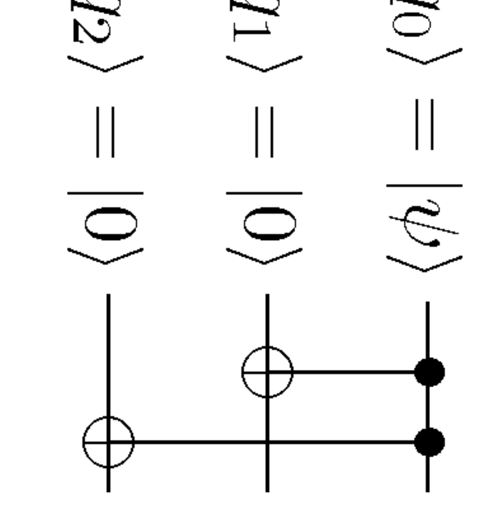
The original qubit can be recovered from the encoded qubit using the following two step process.
- 1.
Error Detection: We perform a measurement that projects the encoded qubit onto a basis that is determined by the errors we want to detect and correct. The measurement result is called the error syndrome, and tells us what error has occurred on the quantum state. For the bit flip channel there are four error syndromes, corresponding to the four projection operators:
(2.26) If a bit flip occurs on qubit one, so that the encoded state becomes , we find that
(2.27) Therefore the error syndrome will always be 1. Moreover, making the measurement leaves the state unchanged. Similarly, if a bit flip occurs on qubit 2 or 3, then the error syndrome will be 2 or 3, respectively. If no bit flip occurs, then the error syndrome will be 0.
- 2.
Recovery: We then use the value of the error syndrome to decide how to recover the initial state. For example, if the error syndrome is 1, we saw that the first qubit must have been flipped. We then simply flip that qubit again by applying to the first qubit in order to recover the initial state. Similarly, if the error syndrome is 2(3), then we flip the second(third) qubit in order to recover the initial state. If the error syndrome is 0, then we do nothing.
As long as a bit flip occurs on no more than one qubit, then this method works perfectly to recover the original state.
The Phase Flip Code
The bit flip code described above is very similar to a classical error-correcting code. A quantum error-correcting code, however, must also correct uniquely quantum errors, such as the phase flip. This error has no classical analogue, as the notion of a phase does not exist in classical information. The phase flip code can detect and correct errors when the input qubit passes through the following channel: the state is taken to the state with probability , and remains unchanged with probability . Since the Pauli operator takes and , it flips the relative phase of the computational basis states. Therefore, this channel is called the phase flip channel.
A three qubit phase flip code can be defined analogously to the bit flip code by passing to a new basis, with basis states and defined by:
| (2.28) |
We can study how the phase flip channel acts on this basis by determining how the Pauli operator acts on the basis states. We see that takes and . Therefore, the channel acts exactly like the bit flip channel, but with the states and corresponding to the classical 0 and 1 its respectively, instead of the computational basis states and .
This information allows us to define a simple three qubit phase flip code analogously to the three qubit bit flip code. First, we note that the Hadamard gate carries out the change of basis from to and vice versa, as the Hadamard gate is its own inverse. We can them implement the phase flip code by applying the Hadamard operation to all the qubits in the system at the appropriate points to switch back and forth between the bases.
The logical basis states and become and respectively. Therefore, the qubit becomes:
| (2.29) |
The quantum circuit shown in Figure 2.7 carries out this encoding. It is the same circuit shown in Figure 2.6 for encoding using the bit flip code, but followed by acting with the Hadamard gate on each qubit to convert to the basis.

The original qubit can be recovered from the encoded qubit using the following two step process.
- 1.
Error Detection: We use the error syndromes , where are the error syndromes for the bit flip channel given by Eq. 2.26.
(2.30) If a phase flip occurs on qubit one, so that the encoded state becomes
, we find that(2.31) Therefore the error syndrome will always be 1. Moreover, making the measurement leaves the state unchanged. Similarly, if a phase flip occurs on qubit 2 or 3, then the error syndrome will be 2 or 3, respectively. If no phase flip occurs, then the error syndrome will be 0.
- 2.
Recovery: We then use the value of the error syndrome to recover the initial state. For example, if the error syndrome is 1, a phase flip must have occurred on the first qubit. We then simply reverse that phase flip by applying to the first qubit in order to recover the initial state. Similarly, if the error syndrome is 2(3), then we reverse the phase flip on the second(third) qubit in order to recover the initial state. If the error syndrome is 0, then we do nothing.
The Shor Code
Although the phase flip code described in Section 2.2.1 corrects phase flips, which are uniquely quantum errors, it is very similar to the bit flip code, which in turn is not very different from classical error-correcting codes. However, there are many more sophisticated quantum error-correcting codes which are truly quantum in nature: that is, they can correct errors that are superpositions of bit and phase flips, and they can correct arbitrary errors on a single qubit.
One example of such a code is the Shor code, which is a combination of the three qubit phase flip and bit flip codes described in Sections 2.2.1–2.2.1. The computational basis states are first encoded using the phase flip code as follows:
| (2.32) |
Each of these three qubits is then encoded using the three qubit bit flip code, as follows:
| (2.33) |
The code is therefore defined by the codewords:
| (2.34) |
Figure 2.8 shows the encoding circuit for the Shor code. The circuit first encodes the input qubit using the three qubit phase flip code, using the circuit shown in Figure 2.7. The circuit then encodes each of these three qubits using the three qubit bit flip code, using the circuit shown in Figure 2.6.

The Shor code allows for the detection and correction of both bit and phase flip errors, as long as the errors only occur on one qubit. In fact, it turns out that the Shor code protects against arbitrary errors, as long as they only affect a single qubit. This illustrates a fundamental difference between quantum and classical error-correcting codes. In the case of quantum error-correction, a continuum of errors that can occur on a single qubit can be corrected by correcting only a discrete subset of those errors (in this case, bit and phase flips.) This concept is known as the discretization of errors. Quantum codes can also correct errors which are slight rotations on more than one qubit, by projecting the erroneous state with some probability onto a state with a single qubit error.
2.2.2 General theory of error correcting codes
In this section we briefly review the general theory of quantum error-correcting codes (QECCs). A quantum error-correcting code is formally defined as a vector subspace of a larger Hilbert space . We let denote the projector onto the codespace . For the three qubit flip code defined above, the projector .
The input quantum states are encoded by a unitary operation into the QECC, and after this encoding process the code is subjected to noise. A syndrome measurement is then carried out to determine what type of error occurred, and the necessary recovery operation is performed to restore the QECC to its original state. The information is then decoded to recover the original information. In order to be able to distinguish the different types of errors that occur, the different error syndromes must correspond to orthogonal subspaces of the original Hilbert space. Otherwise, the errors cannot be distinguished using the syndrome measurement. Furthermore, the errors must map the original orthogonal codewords to orthogonal states, in order to be able to recover from the error.
2.2.3 Stabilizer codes and the Stabilizer formalism
In this thesis we focus on a particular class of well known quantum error-correcting codes (QECCs) known as stabilizer codes [Got97]. We begin by describing the stabilizer formalism, a powerful mathematical framework for describing and manipulating stabilizer codes.
We say that an -qubit state is stabilized by an element of the -qubit Pauli group if . Now, if is a subgroup of , we can define to be the set of all -qubit states that are stabilized by every element of . We then say that is the vector space stabilized by , and is the stabilizer of . We can make these ideas more concrete by giving a simple example. Let . It is easy to check that is a subgroup of . By trial and error we can also check that the vector space spanned by and is the vector space stabilized by .
We do not have to give all the elements in to find . A set of elements is said to generate a group if every element of can be written as a product of elements from . We use the notation to denote that is generated by the set . It is easy to see that if a state is stabilized by all the generators of , then it is generated by all the elements of .
It turns out that if is an abelian subgroup of the -qubit Pauli group that does not contain , then stabilizes a non-trivial vector subspace of the entire -qubit Hilbert space. We call a stabilizer, and the subspace the stabilizer code corresponding to . The dimension of is for some integer , where is the smallest number of generators needed to generate . A dimensional stabilizer code encodes qubits. The weight of an element is equal to the number of that are not equal to the identity. The distance of a stabilizer code is the weight of the minimum weight element in the stabilizer .
2.2.4 Stabilizer states
A stabilizer state is a special case of the stabilizer codes described in Section 2.2.3. Recall that a stabilizer is a subgroup of the -qubit Pauli group that does not contain . If is generated by a minimum of elements of , then defines a dimensional stabilizer code. If , then the stabilizer code is 1-dimensional, and hence there is a unique -qubit state such that for every . Such a state is called a stabilizer state, and the group , also denoted by , is called the stabilizer of . Therefore, a stabilizer state is equivalent to a -dimensional stabilizer code. It has been shown that stabilizer states display genuine quantum entanglement, and considerable efforts have been made to classify the equivalence classes of all stabilizer states under local operations [HDE+06]. Stabilizer states and stabilizer codes are studied further in Chapters 3 and 4.
2.2.5 Stabilizers and Clifford operations
The -qubit Clifford group of unitary operations that map the -qubit Pauli group to itself under conjugation was introduced in Section 2.1.3. In this section we show that the stabilizer formalism provides a simple way of characterizing the action of Clifford operations on a stabilizer code.
Let be an -qubit stabilizer, and an arbitrary state in the subspace stabilized by . Then for all we have
| (2.35) |
Now, let be an arbitrary element of the -qubit Clifford group. Acting on with gives a new state . Then for all we have
| (2.36) |
It follows that the set stabilizes . Moreover, since is a Clifford operation, every element belongs to . As a result the set is a subgroup of , and hence is itself a valid stabilizer. Therefore, we find that Clifford operations map stabilizers to stabilizers under conjugation. It follows that we can equate acting on a stabilizer code with a Clifford operation, and conjugation of the stabilizer by the same Clifford operation. This notion is extremely useful in dealing with stabilizer codes, as it is often much easier to consider the transformations of stabilizers rather than stabilizer codes and states.
Chapter 3 Local Unitary vs. Local Clifford Equivalence of Stabilizer States
In this chapter we study the local Unitary (LU) vs. local Clifford (LC) equivalence problem for stabilizer states. We use graph states to prove that LU-LC equivalence holds for certain classes of stabilizer states, and also report numerical results from the analysis of graph states corresponding to graphs with up to 11 vertices. Much of the original work in this section is reported in [ZCCC07].
In Section 3.1 we present the background information necessary to understand the work in this Chapter. In Section 3.2 we provide some motivation for studying the LU-LC equivalence problem, and in Section 3.3 we formally introduce the problem itself. All of the material up to this point is review of existing results. New results are presented in Section 3.5. In Section 3.5.1 we present our theoretical results, and in Section 3.5.3 we present our numerical results. In Section 3.6 we describe the software that we wrote and used in order to obtain our numerical results. We conclude with a discussion of open problems and suggestions for further work in Section 3.7.
3.1 Background Information
In this Section we introduce the necessary background information on stabilizer states and graph states in order to understand the results in this Chapter.
3.1.1 Stabilizer States
We discussed the problem of classifying stabilizer states in the Introduction, and introduced formal definitions and notation for describing stabilizer states in Section 2.2.3. In this section we first describe two classes of local operations on stabilizer states: local unitary and local Clifford operations. We then introduce a special subset of stabilizer states, known as graph states due to their association with mathematical graphs, that will be used to derive many of the results in this Chapter.
Operations on stabilizer states
In this section we define the local unitary operations and the local Clifford operations. A local unitary (LU) operation on an -qubit state is an -qubit unitary operation can be written as a tensor product
| (3.1) |
of one-qubit unitary operations . Two -qubit stabilizer states and are said to be local unitary (LU) equivalent if there exists an LU operation such that .
An -qubit LU operation that belongs to the -qubit Clifford group is called an -qubit local Clifford (LC) operation. By definition, an -qubit LC operation can be written as a tensor product
| (3.2) |
of one-qubit Clifford operations . Two -qubit stabilizer states and are said to be local Clifford (LC) equivalent if there exists an LU operation in the Clifford group such that .
3.1.2 Graph states
Graph states are a special kind of stabilizer state associated with graphs [HDE+06, SW02]. A graph consists of two types of elements, namely vertices () and edges (). Every edge has two endpoints in the set of vertices, and is said to connect or join the two endpoints. The degree of a vertex is the number of edges ending at that vertex. A path in a graph is a sequence of vertices such that from each vertex in the sequence there is an edge to the next vertex in the sequence. A cycle is a path such that the start vertex and end vertex are the same. The length of a cycle is the number of edges that the cycle has.
For every graph with vertices, we can define a corresponding -qubit stabilizer state in the following way. Given , there are operators for defined by
| (3.3) |
It is straightforward to show that any two s commute, and hence the group generated by is a stabilizer group and stabilizes a unique -qubit state . This is the stabilizer state associated with the graph . We call each the standard generator associated with vertex of graph . Figure 3.1 gives an example of a graph and the standard generators of its corresponding graph state. Throughout the paper we use to denote the unique stabilizer state corresponding to a given graph . It has been shown that any stabilizer state is local Clifford (LC) equivalent to some graph states [dNDM04a].
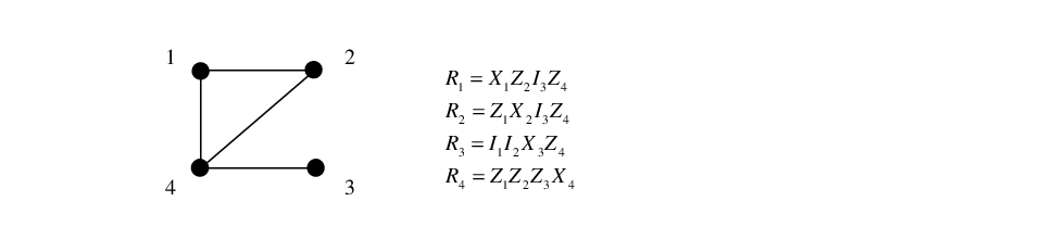
In Section 2.2.3 we saw that the distance of a stabilizer state is the weight of the minimum weight element in its stabilizer. It follows from this definition that a graph state of distance corresponds to a graph with at least one vertex of degree one. Such a vertex will be connected to one other vertex , and the standard generator corresponding to will have the form , which clearly has weight .
3.2 Motivation: Classifying stabilizer states
In this chapter we tackle the first of the three main problems concerning entangled states that were described in the Introduction: Classifying Entangled States. The relation of this chapter to the rest of the thesis is summarized in Figure 3.2.

Despite their importance in quantum information science, multipartite entangled states are still far from being well understood [NC04]. Stabilizer states form a particularly interesting class of multipartite entangled states, which play important roles in areas as diverse as quantum error correction [Got97], measurement-based quantum computing, and cryptographic protocols [RBB03, DAB03, HEB04, HDE+06]. The study of multipartite entanglement has usually focused on determining the equivalence classes of entangled states under local operations, but there are too many such equivalence classes under local unitary (LU) operations for a direct classification to be practical. The most commonly studied set of local operations are the invertible stochastic local operations assisted with classical communication (SLOCC), which yield a much smaller number of equivalence classes. For example, for three qubits, there are only two classes of fully entangled states under SLOCC, while real parameters are needed to specify the equivalence classes under LU operations [VC00, AAC00]. However, the number of parameters needed to specify the equivalence classes under SLOCC grows exponentially with , where is the number of qubits, so that specifying the equivalence classes for all states rapidly becomes impractical for [VDMV02].
For stabilizer states, a more tractable set of operations to study is the local Clifford (LC) group described in Section 3.1.1, which consists of the local unitary operations that map the Pauli group to itself under conjugation. In addition to forming a smaller class of operations, the local Clifford group has the advantage that the transformation of stabilizer states under LC operations can be reduced to linear algebra over , as described in Section 3.6.1. This greatly simplifies all the computations involved in manipulating stabilizer states[HDE+06]. Ideally, we would like to determine the equivalence classes of stablizer states under LC operations, and show that these equivalence classes are, in fact, identical to the equivalence classes of stabilizer states under LU operations. Such a result would allow us to use the simplified framework of the LC operations to study stabilizer states, while retaining the much larger class of transformations allowed by LU operations. This desire leads naturally to the LU-LC equivalence conjecture, described in Section 3.3.
3.3 The Problem
It has been conjectured that any two stabilizer states that are LU equivalent are also LC equivalent. We will often use the notation to denote that this conjecture holds for a particular state, or class of states. If this conjecture is true for all states, then all of the advantages of working with the local Clifford group would be preserved when studying equivalences under an arbitrary local unitary operation. Due to its far-reaching consequences, proving that the equivalence holds for all stabilizer states was until recently one of the most important open problems in quantum information theory. Although a counter-example for the conjecture was found after the work carried out in this thesis [JCWY07], the problem of LU-LC equivalence remains a promising and active area of investigation in this field, as described in Section 3.7.
In this thesis we describe attempts to prove the LU-LC conjecture using graph states, which have proved to be an extremely useful tool in the study of stabilizer states. As every stabilizer state is LC-equivalent to some graph state, proving that holds for all graph states would be sufficient to prove that the conjecture holds for all stabilizer states. Furthermore, it has been shown that an LC operation acting on a graph state can be realized as a simple local transformation of the corresponding graph, and that the orbits of graphs under such local transformations can be calculated efficiently [dNDM04a, DP06, dNM05]. These results indicate that graph states are a natural starting point for investigating the LU-LC problem, since any questions concerning stabilizer states can be restated in graph theoretic terms by invoking the LC-equivalence to graph states. This would make it possible to use tools from graph theory and combinatorics to study the entanglement properties of stabilizer states, and to tackle problems which may have been too difficult to solve using more traditional approaches.
An important step toward a proof of the LU-LC conjecture was taken by Van den Nest et al. [dNDM05], who have shown that two LU-equivalent stabilizer states are also equivalent under LC operations if they satisfy a certain condition, known as the Minimal Support Condition (MSC), which ensures that their stabilizers possess some sufficiently rich structure. They also conjectured that states that did not satisfy the MSC would be rare, and therefore difficult to find. In Section 3.4 we introduce some background material on these results. In Section 3.5 we describe our own work on the LU-LC conjecture. Section 3.5.1 describes our theoretical results, and Section 3.5.3 describes our numerical results. Section 3.6 describes the software that was written in order to analyze graph and stabilizer states, and obtain our numerical results. We conclude in Section 3.7 with a discussion of our results and suggestions for further work.
3.4 Minimal Supports and the Minimal Support Condition
In this section we introduce some background information and notation concerning the detailed structure of stabilizers that is necessary to understand the work in Section 3.5.
The notion of minimal supports has proved to be highly useful in analyzing the properties of stabilizers [Rai99, dNDM05]. Let denote the set of positive integers from 1 to . The support of an element is the set of all such that differs from the identity. Tracing out all qubits of outside gives the mixed state
| (3.4) |
Using the notation , it follows from that
| (3.5) |
A minimal support of is a set such that there exists an element in with support , but there exist no elements with support strictly contained in . An element in with minimal support is called a minimal element.
We now present some results concerning minimal supports that will be useful in understanding the results in this section. We denote by the number of elements with . Note that is invariant under LU operations [dNDM05]. We use to denote the subgroup of generated by all the minimal elements. The following Lemma is given in [dNDM05].
Lemma 3-1: Let be a stabilizer state and let be a minimal support of . Then is equal to 1 or 3 and the latter case can only occur if is even.
Proof: By definition, there must be some element of with support , so if there are no more, . If there are two elements with support , then their product must have support too, as otherwise is not minimal. So cannot be 2, but it can be 3. Suppose there is a fourth element with support . There are only three nonidentity Pauli operators, so one of them must appear twice at some coordinate in . But then we can form another product whose support is strictly contained in , meaning that is not a minimal support, so cannot be greater than 3. Notice that when , must be even, otherwise the operators will not commute.
If is a minimal support of , it follows from the proof of Lemma 3-1 in [dNDM05] that the minimal elements with support , up to an LC operation, must have one of the following two forms:
| (3.6) |
Eqs.(3.4), (3.5) and (3.6) directly lead to the following Fact 3-1, which was originally proved by Rains in [Rai99]:
Fact 3-1: If and are LU equivalent stabilizer states, i.e. , then for each minimal support , the equivalence must take the group generated by all the minimal elements of support in to the corresponding group generated by all the minimal elements of support in .
Based on the above Fact 3-1, the following Theorem 3-1 was proved in [dNDM05] as their main result:
Theorem 3-1: Let be a fully entangled stabilizer state for which all three Pauli matrices occur on every qubit in . Then every stabilizer state which is LU equivalent to must also be LC equivalent to .
The condition given in Theorem 3-1, that all three Pauli matrices occur on every qubit in , is called the Minimal Support Condition (MSC).
For any LU operation which maps another stabilizer state to the stabilizer state , the proof of Theorem 3-1 further specifies the following
Fact 3-2: If all three Pauli matrices occur on the th qubit in , then must be a Clifford operation. Therefore, if the MSC is satisfied for , then must be an LC operation.
3.5 My Work
In this section we extend the work of Van den Nest et al. in [dNDM05] by using graph states to prove that the equivalence holds for all stabilizer states whose corresponding graphs contain neither cycles of length 3 nor 4. This is our Main Theorem. We then give some results complementary to those of Van den Nest et al. We prove that any stabilizer state with distance fails to satisfy the MSC, contrary to the prediction that such states would be difficult to find [dNDM05]. We also prove that all stabilizer states with that satisfy the hypotheses of our Main Theorem also satisfy the MSC. Finally, even though all stabilizer states with distance fail to satisfy the MSC, we show that equivalence can still hold for some of these states if they satisfy certain other technical conditions.
In Section 3.5.3 we provide explicit examples of stabilizer states with distance that fail to satisfy the MSC, and identify all 58 graphs of up to 11 vertices that do not meet this condition. We also describe various other numerical results that were obtained from our study of graph states. Finally, in Section 3.6 we describe the computer programs that we wrote in order to obtain these results. The MATLAB code and User Guide for these programs are given in Appendix A.
3.5.1 Theoretical Results
Our theoretical results are summarized below.
- 1.
equivalence holds for any graph state whose corresponding graph contains neither cycles of length 3 nor 4. This is given as the Main Theorem in Section 3.5.1.
- 2.
The Minimal Support Condition holds for all stabilizer states of distance that satisfy the hypotheses of our Main Theorem. This is given as Lemma 3-3 in Section 3.5.1.
- 3.
All stabilizer states of distance are beyond the Minimal Support Condition. This is given as Proposition 3-1 in Section 3.5.1.
- 4.
equivalence holds for any graph state of distance if the corresponding graph satisfies the Minimal Support Condition after all of its degree 2 vertices have been deleted. This is given as Theorem 3-2 in Section 3.5.2.
Our classification of stabilizer states is summarized in Figure 3.3, which illustrates the relationship between the subsets covered by our results and those of Van den Nest et al., as well as those states for which the problem of equivalence remains open.

The Main Theorem
We now present the new criterion we have found for the equivalence of graph states, which is encapsulated in the Main Theorem stated below.
Main Theorem: equivalence holds for any graph state whose corresponding graph contains neither cycles of length 3 nor 4.
Proof Outline: In order to prove that holds for , where has vertices, we will show that for any -qubit stabilizer state satisfying , there exists an LC operation such that . We prove this theorem constructively, i.e. we construct explicitly from the given , , and . The proof is presented in Sections 3.5.1, 3.5.1, 3.5.1, and 3.5.1. An algorithm for constructing the LC operation is given in Section 3.5.2.
Before giving the details of our proof, we give a brief outline of our strategy. We will use the terms “graph” and “graph state” interchangeably to refer either to the graph itself, or to the corresponding graph state. First, we show that any graph of distance that satisfies the conditions of our Main Theorem also satisfies the MSC, and hence holds for such a graph. However, we will also show that any graph of distance is beyond the MSC. Therefore, we only need to prove the Main Theorem for graphs.
We will assume throughout the remainder of Section 3.5.1 that we are dealing with two graph states and satisfying the conditions of our Main Theorem. The states and are -qubit states (hence their corresponding graphs and have vertices, as each qubit corresponds to a vertex), and are related by the LU operation such that .
We partition the vertex set of graph into subsets as defined later. We show that for all vertices , the corresponding -qubit operator in must be a Clifford operation, i.e. . For vertices , we will give a procedure, called the standard procedure, for constructing . In effect, this corresponds to an “encoding” of any vertex and all the degree one vertices to which is connected into a repetition code (i.e. “deleting” the degree one vertices from ), and then a “decoding” of the code.
We illustrate the proof idea in Figure 3.4. Due to some technical reasons, we first show that for all in Section 3.5.1. We then give the standard procedure in Section 3.5.1. We use an example to show explicitly how the procedure works, with explanations of why this procedure actually works in general. Finally, in Section 3.5.1 we show that for all , and construct for all from the standard procedure.

The four types of vertices we use for a graph are defined as follows.
- 1.
is the degree one vertices of .
- 2.
is the set of vertices is directly connected to some .
- 3.
is the set of vertices not in , and is only connected to .
- 4.
is the set of vertices .
For convenience, we also apply this partitioning of vertices to graphs. Since such graphs contain no degree 1 vertices, for a graph of distance we have . Figure 3.5 gives an example of such partitions.

and graphs and Case
We first provide some lemmas which lead to a proof of the Main Theorem for graphs. Then we show that all graphs are beyond the MSC.
graphs
Lemma 3-2: For a vertex which is unconnected to any degree one vertex, if it is neither in cycles of length nor , and then is the only minimal element of support .
Proof: Suppose the vertex connects to vertices . Then . If there exists an element such that , then must be expressed as a product of elements in . However since is not in any cycle of length or , then any product of elements in (except itself) must contain at least one Pauli operator acting on the th qubit where is not in .
This directly leads to the following Lemma 3-3 for graphs:
Lemma 3-3: For any graph with , if there are neither cycles of length nor , then satisfies the MSC, and hence holds for .
Proof: Since , then all vertices are unconnected to any degree one vertices. Then by Lemma 3-2 we find that , and therefore the MSC is satisfied.
Lemma 3-3 shows that we only need to prove the Main Theorem for graphs of . Furthermore, Lemma 3-2 tells us that for any vertex , we must have , according to Fact 3-2. Therefore, to construct the LC operation , we can take for all .
graphs
Proposition 3-1: Stabilizer states with distance are beyond the MSC.
Proof: A stabilizer state with has at least one weight two element in its stabilizer . We denote one such weight two element by , where and are one of the three Pauli operators on the th and th qubits respectively, up to an overall phase factor of or . Now consider any element in with a support such that . We can write in the form where each is either the identity matrix or one of the Pauli matrices , up to an overall phase factor of or . Then there are three possibilities: (i) If is or , then since commutes with , the operator () can only be (), up to an overall phase factor of or . (ii) If , then since commutes with , we either have , where anticommutes with and anticommutes with , or . The former is impossible, as the whole graph is connected, so the latter must hold. (iii) If strictly contains , then is not a minimal element. It follows that in , only appears on the th qubit and only appears on the th qubit, showing that is beyond the MSC.
Furthermore, the local unitary operation which maps another stabilizer state to is not necessarily in the Clifford group, particularly on the th and th qubits. Note that it is always true for any angle that
| (3.7) |
To interpret Proposition 3-1 for graph states, note that any fully connected graph with degree one vertices represents a graph state of . Therefore, a graph with degree one vertices is beyond the MSC. In particular, for a graph with neither cycles of length nor , each weight two element in corresponds to the standard generator of a degree one vertex in .
Case : The standard procedure
The main idea behind the standard procedure is to convert the LU-equivalent stabilizer states and into corresponding (LC equivalent) canonical forms for which we can prove by applying “encoding” and “decoding” methods. We can then work backwards from those canonical forms to prove that for .
We use a simple example, as shown in graph B4 of Figure 3.6, to demonstrate how the standard procedure works. The standard procedure decomposes into five steps, given in Sections 3.5.1-3.5.1. In each step, we also explain how the step works for the general case.

Note that is a GHZ state; hence holds. The standard generator of the stabilizer for graph is . However, as we will see later in step 4, for does not guarantee that for .
We now prove that for .
Step 1: Transform into a new basis by LC operation
It is straightforward to show that
| (3.8) |
where , which is determined by the the edge set .
Performing the Hadamard transform on the fourth and fifth qubits, we get
| (3.9) |
where
| (3.10) |
The form of in Eq.(3.9) is not hard to understand. By performing , the standard generator of will be transformed to , hence only the terms of and appear on the qubits . Furthermore, for the supports , we have .
For any other stabilizer state which is LU equivalent to , there exists an LU operation such that . According to Fact 3-1, for the supports , , we must also have . Suppose the minimal elements corresponding to , are , respectively. Then there exist , such that , and . Therefore, we have
| (3.11) | |||||
where and are two states of qubits and .
Then we have
| (3.12) |
where
| (3.13) |
i.e. , , , , .
Eq.(3.12) is then our new starting point, since and are LC equivalent if and only if and are LC equivalent. We can then always get the former when we prove the latter by reversing Eq. (3.13), as we will do from eqs. (3.37) to (3.38).
Note that the procedure of getting Eq.(3.12) is general, i.e. we can always do the same thing for any graph state and its LU equivalent graph states. To be more precise, for a general graph of vertices, consider a vertex , and let be the set of all degree one vertices in which connect to . If the size of this set is , then without loss of generality we can rename the qubits so that the vertices and are represented by the last qubits of .
Applying the Hadamard transform to gives a new stabilizer state as shown below.
| (3.14) | |||||
where and are two states of the other qubits.
Similarly, for any stabilizer state which is LU equivalent to , i.e. , there must exist (for all ) such that
| (3.15) |
for .
Defining , we have
| (3.16) | |||||
where and are two states of the other qubits.
We apply the above procedure for all . Defining and , we get
| (3.17) |
Now define
| (3.18) |
where for all , for all , and for all . We then have .
It can be seen that and are LC equivalent if and only if and are LC equivalent. Therefore, we can use the states and as our new starting point.
Our current situation is summarized in the following diagram.
Step 2: Encode into repetition codes
Now we can encode the qubits , and into a single logical qubit, i.e. and . Define
| (3.19) | |||
| (3.20) |
Then both and are -qubit stabilizer states. In particular, is exactly the graph state represented by the graph . Now Eq.(3.12) becomes
| (3.21) |
where , and is a logical operation acting on the logical qubit, which must be of some special form as we will discuss below. The upper index indicates that we may understand this logical qubit as being the rd qubit in graph .
Due to Fact 3-1, we must have
| (3.22) |
which means that either
| (3.23) |
which gives for some , or
| (3.24) |
which gives , , for some .
Note that the procedure of getting Eq.(3.21), and the resulting possible forms of are also general. To see this, recall that if we have two states of the form given in Eq. (3.14) and Eq. (3.16), we can encode the qubits and into a single logical qubit, by writing and . We can then define two new stabilizer states and , given by
| (3.25) |
Both are stabilizer states of qubits, where . In particular, is represented by a graph which is obtained by deleting all the vertices from .
We can see that and are related by
| (3.26) |
where , and is a logical operation acting on the logical qubit .
Similarly, we can place some restrictions on the form taken by . By Fact 3-1, we have
| (3.27) |
for all . This means that either
| (3.28) |
for all and some , which gives
| (3.29) |
where , or
| (3.30) |
for all and some , which gives
| (3.31) |
where .
Now, we once again apply the above encoding procedure to all . This leads to two -qubit stabilizer states and , where . In particular, is represented by a graph which is obtained by deleting all the degree one vertices from . Defining
| (3.32) |
we have
| (3.33) |
After this step of our standard procedure, our situation is as shown below:
Step 3: Show that
We then go on to show that , which means that . To see this, consider the minimal element , which is the standard generator of graph associated with the (logical) qubit . Then holds for both and . Furthermore, is the only minimal element of according to Proposition 3-1. If is not in , then for any , which contradicts Fact 3-1. It is not hard to see that the fact of is also general.
We now show that can also be induced by local Clifford operations on the qubits . This can be simply given by if Eq.(3.23) holds, or if Eq.(3.24) holds.
In the general case, it is shown in Lemma 3-2 that for a graph with neither cycles of length nor , the standard generator of any vertex which is unconnected to degree one vertices will be the only minimal element of . Then due to the form of in Eq.(3.31), we conclude that for a general graph with neither cycles of length nor , any induced must be in . Similarly, each can also be induced by local Clifford operations on the qubits . This can be simply given by if Eq.(3.29) holds, or if Eq.(3.31) holds.
Step 4: Construct a logical LC operation relating and
In this step, we start from the general case first and then go back to our example of the graph .
For a general graph , for which and are not both empty sets, we show that for , must be in for any which is not a logical operation. To see this, note that in Section 3.5.1 we have already shown that for all . And we are going to show in Section 3.5.1 that for all . We have also applied Steps 1 and 2 to each to obtain . As shown in Step 3 we have , and hence is an LC operation such that .
Now we go back to our example. Note that for graph , we have already shown that is a Clifford operation. If we could further show that and are also Clifford operations, then is an LC operation which maps to .
However, for graph , , i.e. the vertices and are neither in nor . Then we have to show that although and themselves are not necessarily Clifford operations, there do exist , such that
| (3.34) |
This can be checked straightforwardly due to the simple form of , where . Since we know that is also a -qubit GHZ state, and can only be of very restricted forms. To be more concrete, for instance, for , where , we could have , and , i.e.
| (3.35) |
But we know
| (3.36) |
Note that other possibilities for (and the possible corresponding , and ) can also be checked similarly.
One may ask why we do not also delete the vertex in graph as we do in the general case, which would probably give us a logical Clifford operation on the vertex . Then for the graph with only two vertices and , we would have an LC operation . However, this turns out not to be the case due to the fact that the connected graph of only two qubits is beyond the conditions of our Proposition 3-1. Then in this case the argument in Step 3 no longer holds.
Step 5: Decode to construct
Finally, the remaining steps are natural and also general. We can choose , and choose if or if , which gives
| (3.37) |
where .
Defining , where , , , , and , we get
| (3.38) |
as desired.
In general, for each and all , choose and choose if , or and if . Defining
| (3.39) |
we have
| (3.40) |
Defining , where for all , for each , and for all , then
| (3.41) |
which is desired.
Steps 3, 4, and 5 are then summarized in the following diagram.
Case
Unlike the case of , where is guaranteed by Lemma 3-2 and Fact 3-2, the case of is more subtle. Lemma 3-2 does apply for any , i.e. the standard generator is the only minimal element of . However, for any , the generator is not in due to Proposition 3-1, and hence Fact 3-2 does not apply. We must therefore study the case of vertices in more carefully.
We now use the standard procedure to prove that for all , thereby proving that for . We use to denote the graph obtained by deleting all the degree one vertices from . Note for any , we must have . Then there are three possible types of vertices in :
- Type 1:
,
- Type 2:
,
- Type 3:
.
We discuss the three types in Sections 3.5.1, 3.5.1, and 3.5.1, respectively.
Type 1
The subtlety of proving for a Type 1 vertex is that we need to apply the standard procedure twice to make sure that . We will demonstrate this with the following example, to prove that for graph in Figure 3.7.

For , the standard construction procedure will result in , where for and . We now use the construction procedure once again on qubit of and encode the qubits , into a single qubit , as shown in Figure 3.7 (). This gives , where for . Here is induced by via a similar process as Eqs. (3.12, 3.13, 3.14). Since , we must have , as desired.
In general we can prove that for any Type 1 vertex as we did for vertex in the above example of the graph . To be more precise, let be a vertex of Type 1. For each , carrying out the standard procedure at every gives us a graph . We know that each must be in . Since and , we then have a non-empty . Again for we carry out the standard procedure at , giving us a graph , and each must be in . This gives due to the form of in Eqs.(3.29,3.31).
Type 2
Now we consider the Type 2 vertices. We give an example first, to prove that for the graph in Figure 3.5. is a graph without cycles of length 3 and 4, and represents a general graph with four types of vertices. is very similar to , and has the same set of , , , and as . The only difference between the two graphs is that in , vertices and are connected to each other. Therefore, following the example for the graph shows that for any , the standard construction procedure will result in , where for and . However, from the structure of , it is easy to conclude that .
In general, we can prove that for any Type 2 vertex as we did for vertex in the above example of the graph . To be more precise, let be a vertex of type 2. For each , carrying out the standard procedure at all gives us a graph . contains neither cycles of length nor , so the same holds for . Since , we have . Due to Lemma 3-2, we conclude that .
Type 3
Now we consider the Type 3 vertices. Let us first examine an example. Consider the graph which is obtained by deleting vertices and from graph . For this new graph with , we have , , , and . It is easy to see that the vertex is of Type 3. Carrying out the standard procedure at vertices and gives a graph , which is a subgraph of with . Now we see that , and hence for any which takes the graph state to another -qubit stabilizer state.
In general, note that is of type 3 only when every vertex not only connects to some degree one vertices, but also connects to some vertices in . So the trick is to perform the standard procedure only at all . This gives a graph . Since , we have . Due to our result in Sec. III A1, we conclude that .
Some remarks
To summarize, in general we first classify the vertices of into four classes: , , , and . To construct , we choose for all , and then apply the standard procedure to construct for all .
Note that for some graphs for which and are both empty sets, for instance the graph in Figure 3.6, the general procedure discussed in the above paragraph does not apply directly. This special situation has already been discussed in detail in Section 3.5.1.
This completes our proof of the Main Theorem.
3.5.2 Algorithm for constructing
The proof of our Main Theorem implies a constructive procedure for obtaining the local Clifford operation corresponding to a given local unitary operation . This procedure is described below. For clarity, the operation “” is used to denote standard matrix multiplication in .
Proving LU-LC equivalence for other classes of graph states
In this section, we present a theorem regarding equivalence for graphs. We again use to denote the graph obtained by deleting all the degree one vertices from .
Theorem 3-2: holds for any graph if satisfies the MSC.
Proof: The proof is the same as the proof of the Main Theorem in the special case where is an empty set.
Although the proof of Theorem 3-2 is a special case of the proof of the Main Theorem, Theorem 3-2 is not a corollary of the Main Theorem. It can be applied to many graphs with cycles of length or , since we know that many graphs satisfy the MSC.
3.5.3 Numerical Results
All of the numerical results in this Section were obtained using the MATLAB scripts described in Section 3.6.
Graph States beyond the MSC
From Lemma 3-3, we know that for graphs of distance , our Main Theorem is actually a corollary of Theorem 3-1. An interesting question is: do there exist other graph states with distance which do not satisfy the MSC? The answer is “Yes”, and we now give some examples of such states.
Graphs obtained by numerical search
Generally the distance of a graph state can be upper bounded by for a graph whose elements in have even weight, which only happens when is even. For the other graphs, the distance is upper bounded by , if mod 6, , if mod 6, and , otherwise [RS98].
Our numerical calculations show that there are no graphs beyond the MSC for . Among all the LC non-equivalent connected graphs of , there are only three graphs beyond the MSC. All of them are of distance three, which are shown as graphs A6, B6, and C6 in Figure 3.8. Among all the LC non-equivalent connected graphs of , there are only nine graphs beyond the MSC. Eight of them are of distance three, and only one is of distance four. The distance four graph of beyond the MSC is shown as graph D6 in Figure 3.8. Among all the LC non-equivalent connected graphs of , there are only graphs beyond the MSC. of them are of distance three and are of distance four.

Graphs derived from codes with non-Clifford transversal gates
In [ZCCC07], we construct two other series of graph states beyond the MSC for () from quantum error-correcting codes that are analogous to the classical Reed-Muller codes[FJM77]. The graphs for and were drawn using the software described in Section 3.6, and are given in Figures 3.9 and 3.10.


property for graph states
It is natural to ask whether we could use the same strategy to prove for those graph states beyond the MSC as we did for graphs in Section 3.5.1. However, our numerical investigations suggested that it would be difficult to extend our approach of deleting vertices: and indeed, this intuition appears to have been supported by the discovery of a counterexample for the equivalence conjecture.
We considered the possibility of deleting vertices of degree , as a simple extension of deleting degree one vertices from graphs of distance . In order to see if this inductive approach could be successful, we used the MATLAB scripts described in Section 3.6 to analyze the structure of the stabilizers of graph states for . We found that it is possible for a graph state to satisfy the MSC without satisfying , although examples of such states are rare. We found only two LU-inequivalent examples for , which are shown below in Figure 3.11.

Note that both of the graphs in Figure 3.11 are of . There exist two graphs satisfying the MSC but with for , but there does not exist any such graph with this property for . This interesting phenomenon implies that the structure of is a global rather than a local property of graph states, which cannot be simply characterized by the idea of induction.
3.6 Software for Analysis of Graph States
This section describes the software that I wrote in order to carry out numerical analysis of graph states. The software bundle consists of a set of MATLAB scripts, and can be divided into three groups. In each script, the graph corresponding to a graph state is represented by a symmetric adjacency matrix, where is the number of qubits in the graph state. Each script is described by giving its Input, its Output, and a brief summary of its operation. The software is described in Sections 3.6.2, 3.6.3, and 3.6.4. Many of the scripts use auxiliary scripts, which are described in the Appendix. The algorithms used in the MATLAB scripts rely heavily on the stabilizer formalism, which was introduced in Section 2.2.3. Using the stabilizer formalism, it is possible to simplify all the necessary computations to linear algebra in a binary framework. The necessary background information for these computations is introduced in Section 3.6.1.
3.6.1 Stabilizers using Linear Algebra
Until now, we have described the stabilizer formalism using the language of group theory. In this Section we will exhibit an alternate description of stabilizers using linear algebra over the field . Our exposition closely follows that given in [Got97].
Throughout this section we will consider the stabilizer of an -qubit state . The stabilizer has generators . We can write as two matrices concatenated into a single matrix with entries in , where each row corresponds to a generator, and the th and th columns correspond to the th qubit, as illustrated in Figure 3.12. This matrix is called the check matrix of the stabilizer. This is the binary symplectic form for a stabilizer, obtained by using a group homomorphism between the -qubit Pauli group and the space of binary vectors of length . The homomorphism maps an element to an element , where and are both binary vectors of length . The th entry of is 1 if or , and otherwise. The th entry of is 1 if or , and 0 otherwise [dNDM04b].
This homomorphism gives us a simple recipe for obtaining the check matrix from the generators . Each generator has the form , where each and . As previously mentioned, the th row of the check matrix corresponds to the generator . Ignoring the overall phase factor , the entries in the th row are determined using the following rules.
- 1.
If , then the entry in the th row and th column, and the entry in the th row and the th column, are both 0.
- 2.
If , then the entry in the th row and th column is 1, and the entry in the th row and the th column is 0.
- 3.
If , then the entry in the th row and th column, and the entry in the th row and the th column, are both 1.
- 4.
If , then the entry in the th row and th column is 0, and the entry in the th row and the th column is 1.
Conversely, we can use these rules to write down the generators of a stabilizer from the corresponding check matrix. The binary vector (in this case, the th row of the check matrix) obtained in this way from a stabilizer element is called a codeword. The weight of a codeword is the weight of the corresponding stabilizer element, and is equal to the number of non-zero entries in the codeword. An example of a check matrix and its stabilizer is given in Figure 3.12.

. The check matrix is constructed by concatenating two matrices. The left hand matrix corresponds to the operators, and the right hand matrix corresponds to the operators. Each row corresponds to a generator, and the th and th columns correspond to the th qubit. If a generator has an () at the th qubit then the entry in the th(th) column of the corresponding row is a 1. Otherwise, the entry is a 0. If a generator has a at the th qubit then the entry at the th and th columns are both 1.
We can see that the check matrix can be written in the block matrix form , with the matrix on the left corresponding to the Pauli- matrices, and the matrix on the right corresponding to the Pauli- matrices. If the stabilizer generator corresponding to the th row has an () on the th qubit, then the entry in the th row and th column of () is 1.
The condition that the stabilizer be an abelian group is equivalent to the condition that the check matrix should satisfy
| (3.42) |
for all . This is equivalent to the condition that the check matrix should satisfy
| (3.43) |
for the matrix defined by:
In Section 2.2.5 we saw that by using the stabilizer formalism we could equate acting on a stabilizer state with a local Clifford operation, and conjugation of the stabilizer by the same LC operation. In this linear algebra framework it turns out that all LC operations can be reduced to operations on the check matrix over the field . For example, acting with the Hadamard gate on the th qubit corresponds to exchanging the th and th columns of the check matrix, as
| (3.46) | ||||
| (3.47) |
From the description of the standard generators for the stabilizer of a graph state in Section 3.1.2, we can see that the corresponding check matrix can be written in the block matrix form , where is the identity matrix and is the adjacency matrix of the corresponding graph.
In the remaining Sections we describe the MATLAB scripts written to obtain the numerical results in this Chapter. Figures 3.15, 3.13, and 3.14 show module dependency diagrams depicting the relationships between the routines described in this section and the auxiliary scripts given in the Appendix. Some routines are shown in more than one figure for clarity.


3.6.2 Basic Graph State Manipulation
The scripts described in this section allow the user to convert a stabilizer state into an LC-equivalent graph state, and then carry out simple manipulations and analysis of the graph state.
Obtaining an LC-equivalent graph state of a stabilizer state
Name: Stab2Graph
Input: A character array containing the stabilizer generators of an -qubit stabilizer state.
Output: An adjacency matrix for the graph representing an LC-equivalent graph state, and a drawing of the graph.
Operation: The script Stab2Graph()is used to calculate an LC-equivalent graph state given a stabilizer state specified by its stabilizer generators. The graph state is calculated by representing the stabilizers in a check matrix, then converting the check matrix to a “standard form” used to represent the stabilizers of graph states using valid LC operations [dNDM04a].
The program takes as its input a list of stabilizers, which is assumed to be a character array containing the stabilizer generators in the form . For example, if the stabilizer generators were , then the user would enter:
A = [’XXX’; ’IZZ’; ’ZZI’];
at the MATLAB prompt.
The program first determines the number of qubits in the state, , which is the length of each stabilizer generator. It then creates a check matrix corresponding to the stabilizer generators, and row reduces the check matrix over the field using the auxiliary script rowRedMod2(). The check matrix is in the form , where each row corresponds to a binary vector representing a stabilizer element of an qubit state as described in Section 3.6.1.
The auxiliary script GetCheckMatrix()is used to find the check matrix. This script expects an input of the same form as the character array above, and returns the check matrix obtained by converting each element in the array into the corresponding binary vector. Stab2Graph()then deletes any zero rows from the check matrix and verifies that the resulting matrix is . If it is not, then the stabilizers do not define a stabilizer state and an error message is returned.
The program then checks to make sure that all of the generators commute with each other, which is necessary for the generators to define a stabilizer state. If the stabilizer generators pass all of these checks, then the corresponding LC-equivalent graph state is computed using the auxiliary script findGraph(cMat).
The script findGraph(cMat)expects an check matrix as an input, and calculates the adjacency matrix of an LC-equivalent graph state of the stabilizer state given by the check matrix. Note that the graph state found by this script is not unique, as a single stabilizer state can have many LC-equivalent graph states.
The program assumes that the check matrix cMat is given in the form , and carries out Gaussian row reduction in to give a new basis for the stabilizer. Row reduction is carried out using the auxiliary script rowRedMod2(). This gives a matrix of the form:
The program then calculates , and switches columns of the left and right hand sides. This is a valid LC operation, equivalent to the Hadamard operation on qubits .
This gives a matrix of the form , where is invertible. The program then uses Gaussian elimination again to row-reduce the matrix. This finally gives us the standard form for the check matrix of a graph state, where G is the adjacency matrix. The program outputs the adjacency matrix G and plots the graph, labeling the vertices from to .
There are two versions of the programs Stab2Graph()and findGraph(cMat), as they both have versions designed to work with the graphical user interface described in Section 3.6.2 (Stab2GraphGUI()and findGraphGUI(cMat)). The versions only differ in the way they output error messages. The first versions, which are designed to be run directly from the Matlab prompt, return an error message to the Matlab console. The versions which are called by the graphical user interface return an error message as the output of the function, which is then displayed on the GUI.
Local Complementation
Name: LocalComp()
Input: An adjacency matrix for a graph, and the index of a vertex in the graph.
Output: An adjacency matrix representing the graph after local complementation at vertex .
Operation: It has been proved that the orbit of a graph state under local Clifford operations can be generated by a simple graph transformation known as local complementation [HDE+06]. This means that every LC operation on a graph state is a composition of local complementation operations. A local complementation operation at vertex in a graph replaces the subgraph of induced by with its complement. An example of local complementation is shown in Figure 3.16.

The function LocalComp()takes as its inputs the adjacency matrix of a graph, , and the index of the vertex at which to carry out local complementation. Local complementation is carried out at this vertex and the new adjacency matrix is given as the output, which is calculated using the formula [dNDM04a]:
| (3.50) |
The diagonal entries in the output are set to zero so that there are no self-loops. is the matrix with a 1 in the th diagonal entry and zeros elsewhere. An adjacency matrix can be entered as an ordinary matrix, with only 0 and 1 entries. An example of a graph and its adjacency matrix is shown in Figure 3.17.

Measurements on Qubits
Name: MeasureQubit()
Input:
- •
, the adjacency matrix of the initial graph state.
- •
, the index of the vertex where the measurement is carried out ().
- •
, a letter indicating which measurement is being carried out ().
- •
, the index of a neighboring vertex in the case that , as such a vertex needs to be specified in the case of an measurement.
Output: The adjacency matrix of a graph state after a measurement has been carried out on qubit .
Operation: The program allows the user to carry out Pauli measurements on the qubits of the graph state. It has been proved that the state which results from carrying out , and measurements on the th qubit can be derived from the original graph by a series of simple graph operations, without reference to the stabilizer [HDE+06]. Therefore, if the user had defined a graph using an adjacency matrix , and wanted to make a measurement at vertex 1, they would enter:
MeasureQubit(G, 1, Z, 1);
Note that when the measurement is not an -measurement, can take any value.
The function calculates the output adjacency matrix for the measurements as follows [dNDM04a]:
- •
A -measurement at vertex is equivalent to making an isolated vertex. The output adjacency matrix is therefore calculated by setting the entries of the th row and column to 0.
- •
A -measurement at vertex is equivalent to local complementation at vertex followed by a -measurement at vertex . Local complementation is carried out by calling the function LocalComp()described in Section 3.6.2, where is the adjacency matrix of the graph and is the vertex at which to carry out local complementation.
- •
An -measurement at vertex is equivalent to local complementation at a neighbor of , followed by a -measurement at vertex , then another local complementation at vertex . If is an isolated vertex, the state is left unchanged.
Calculating the Schmidt Rank for bipartitions
Name: findSchmidtRank()
Input: The adjacency matrix of a graph corresponding to a graph state, and a subset of the vertices defining a bipartition.
Output: The Schmidt rank of the graph state calculated as shown below, with respect to the bipartition defined by .
Operation: The Schmidt Rank of a state is often used as a measure of entanglement [FCY+04]. Although it is difficult to calculate for partitions of the qubits into more than 2 sets, it is fairly easy to calculate for a bipartition of the vertices of a graph state. The user specifies one subset of the vertices, and the program findSchmidtRank()calculates the Schmidt rank for the bipartition where .
is given as a row vector of vertex indices. So if the user had a graph with 5 vertices defined using the adjacency matrix , and they wanted to calculate the Schmidt rank for the bipartition , they would enter:
A = [1 2 3];
findSchmidtRank(G,A);
The adjacency matrix can be rewritten using row and column permutations so that the first rows and columns correspond to vertices in , and the last rows and columns correspond to vertices in . Then takes the form:
where () denotes a sub-matrix that shows edges connecting only vertices in (), and denotes a sub-matrix that shows edges connecting a vertex in to a vertex in . The matrix is the transpose of the matrix . The program calculates by selecting the rows of corresponding to vertices in and the columns of corresponding to vertices in . The Schmidt rank is then the rank of over , which is calculated using the auxiliary script rowRedMod2() [HDE+06].
Entanglement Measures
Name: findEntanglement()
Input: The adjacency matrix of a graph corresponding to a graph state, and a partition of the vertices.
Output: A measure of the entanglement of this graph state calculated as described below, with respect to the partition .
Operation: A new measure for the entanglement of stabilizer states has been proposed [FCY+04], which is easier to calculate than the Schmidt rank described in Section 3.6.2. The function findEntanglement()calculates this entanglement measure for a graph state, where is the adjacency matrix of the graph and is the character array which describes a partition of the vertices .
In order to be a valid partition, must satisfy:
- •
, and
- •
for all .
For example, if had 5 vertices and the partition was , then P would be entered as:
P = [’1’; ’2’; ’345’];
If is the stabilizer of the graph state, then consists of the elements of which act as the identity on the subset of .
If the inputs are valid, then the program goes through each partition in turn, and uses the auxiliary script findIdOnA()to determine the generators of . The program then concatenates the generators for all the into a single check matrix, then row reduces this check matrix over to find the generators of the product group .
The value of the entanglement measure is given by:
| (3.53) |
where represents the rank of a group , which is the number of generators of . In this case is the rank of the product group , which is the rank of the check matrix found by concatenating the generators for every .
The auxiliary script findIdOnA()takes as its inputs an adjacency matrix representing a graph state, and a set of indices which indicates a subset of the vertices of . The script returns a check matrix containing the generators of a subset of the stabilizer ( is defined above as the elements of which act as the identity on the subset of .) A general element of the stabilizer acts as the identity on if and only if the following conditions are met [FCY+04]:
- •
for all .
- •
For all , has an even number of indices such that is not the identity.
The program goes through all the elements of the stabilizer and finds those elements which satisfy this condition for all vertices in . It then concatenates all these elements into a check matrix, and row reduces the check matrix to find the generators of .
The Graphical User Interface
All of the scripts described in this section can also be run using a graphical user interface (GUI), which is launched by entering:
StabToGraphv1();
at the MATLAB prompt. The script StabToGraphv1uses an auxiliary script Stab2GraphGUI, given in the Appendix, which is identical to the script Stab2Graphdescribed in Section 3.6.2 except for the way in which it handles error messages. The script Stab2GraphGUIdoes not output error messages to the MATLAB prompt. Instead, it returns a string containing the error message that can be displayed on the GUI.
The GUI displays instructions for using the various features, and also has a “Reset” button that clears the current graph state and all calculations, so that the user can specify a new set of stabilizers to study. The GUI is illustrated in Figure 3.18.

3.6.3 Analysis of a Graph State
The scripts described in this section allow the user to determine basic properties of a graph state, such as its distance.
Determining if a graph state has distance
Name: distanceTwo()
Input: The adjacency matrix of a graph corresponding to a graph state.
Output: A Boolean variable indicating whether or not the graph state has distance .
Operation: The function distanceTwo()determines if the graph state represented by the adjacency matrix has distance . The function first checks to see if contains a degree 1 vertex, which means that it has distance 2, as there is a weight 2 element in the stabilizer. If not, it then checks all codewords , such that is a sum of 2 rows over in the check matrix corresponding to this graph state, to see if there is a codeword of weight 2. G has distance 2 if and only if there is such a codeword.
This is due to the fact that an element in the stabilizer of a graph state which is the product of stabilizer generators has weight [DP06, Dan05]. Here, we are assuming that the stabilizer generators are in the standard form for a graph state, i.e. the stabilizer for qubit is as given below, where is the neighborhood of the vertex in the graph:
| (3.54) |
Finding the distance of a graph state
Name: findDistance()
Input: The adjacency matrix of a graph corresponding to a graph state
Output: The distance of the graph state, which is equivalent to the weight of the element of minimum weight in the stabilizer.
Operation: The function findDistance()finds the distance of the graph state represented by the adjacency matrix . The algorithm used is Algorithm 3.1 from reference [Dan05], and is given below as Algorithm 2( = weight of ).
As before, this algorithm assumes that an element in the stabilizer of a graph state which is the product of stabilizer generators has weight , where the stabilizer generators are in the standard form for a graph state.
Finding the LC orbit of a graph state
Name: findLCOrbit()
Input: The adjacency matrix of a graph corresponding to a graph state, and a parameter disp, which determines whether or not the graphs in the LC orbit are displayed.
Output: A set of adjacency matrices containing all of the graphs in the LC orbit of the input graph.
Operation: The function findLCOrbit(, disp)takes as input the adjacency matrix of a graph , and returns an array of matrices containing the orbit of under local Clifford (or equivalently, local complementation [HDE+06]) operations. The program uses Algorithm 5.1 from [Dan05] to generate the LC orbit of a graph. If the parameter disp=1, the graphs in the orbit are displayed. Otherwise, they are not. The algorithm used to generate the orbit is given here as Algorithm 3 ( is the graph obtained by carrying out local complementation at vertex .) Note that this version of the algorithm differs slightly from the one given in the reference, which uses the program nauty (see [Dan05]) to obtain a canonical representative of each isomorphism class of graphs. This program generates all isomorphisms. There was also a mistake in the published form of the algorithm which was corrected through personal communication with the author.
Determining if a graph is connected
Name: connected()
Input: The adjacency matrix of a graph corresponding to a graph state.
Output: A Boolean variable indicating whether or not the input graph is connected.
Operation: The function connected()tests the adjacency matrix of a graph to see if the graph is connected. It outputs 1 if the graph is connected, and 0 otherwise. The program begins at vertex 1 of the graph, and systematically marks all vertices reachable from this vertex using a breadth-first search. This gives vertices, where is the total number of vertices in the graph, if and only if the graph is connected.
Finding the representative of an LC orbit
Name: findLCRepresentative()
Input: The adjacency matrix of a graph corresponding to a graph state.
Output: An adjacency matrix representing the graph in the LC orbit with the fewest number of edges.
Operation: The script findLCRepresentative()uses the function
findLCOrbit()described in Section 3.6.3 to generate the LC orbit of , then searches through these to find the adjacency matrix representing the graph with the fewest number of edges. This adjacency matrix is returned as the output of findLCRepresentative(). Since we are dealing with simple graphs with no self-loops, the adjacency matrices will all be symmetric with “0”s along the diagonal. Each “1” in an adjacency matrix corresponds to an edge in the graph. Therefore, the sum of all the entries in an adjacency matrix is equal to , where is the set of all the edges in the graph . This makes it easy to calculate the number of edges in a graph represented by an adjacency matrix .
3.6.4 Analysis of Sets of Graph States
The scripts described in this section allow the user to determine the properties of graph states needed to establish LU-LC equivalence. The scripts allow for bulk analysis of graph states represented by adjacency matrices saved in a text file, as well as individual analysis of each graph state.
Generating a text file for bulk analysis of graph states
Name: standardiseLC(, filename)
Input: The number of vertices in the graphs being considered, and the name of a text file containing adjacency matrices for all of the graphs being processed.
Output: A text file StandardLCReps.txt containing an adjacency matrix for each graph in the input file. The output graphs are all chosen to be the graphs in their LC orbits with the fewest edges.
Operation: The script standardiseLC(, filename)expects as input the number of vertices in the graphs being considered, , and the filename of a text file containing the adjacency matrices we are looking at. If the text file were called ‘Graphs.txt’, and the graphs had 5 vertices, the user would type:
standardiseLC(5, Graphs.txt);
The text file should contain one adjacency matrix per LC orbit. This script takes each adjacency matrix, and finds the member of the LC orbit of the corresponding graph with the fewest number of edges using the function findLCRepresentative(). It then outputs a new file called StandardLCReps.txt containing representatives of the same LC orbits, but chosen so that they contain the minimum number of edges. The function also removes any graphs which are not connected, by using the function connected()(see Section 3.6.3.) This script makes it easier to process batches of adjacency matrices by putting each one in a standard form.
Finding the Minimal Generators of a Stabilizer
Name: FindGenSatMSC()
Input: The adjacency matrix of a graph corresponding to a graph state.
Output: A list of indices indicating the vertices which correspond to minimal elements in the stabilizer of the graph state.
Operation: The script FindGenSatMSC()takes as input the adjacency matrix of a graph corresponding to a graph state, and outputs a list of the vertices corresponding to the stabilizers which are minimal elements. The program first finds the standard check matrix for the stabilizer of the graph state, and goes through the stabilizer generators . For each , the program selects the rows of the adjacency matrix representing the generators that could be multiplied to give stabilizer elements whose supports are contained in the support of . The program then calculates all possible combinations of these stabilizers, and searches for one whose support is contained in the support of . If there is no such element, then is minimal. Otherwise, is not minimal. This program uses the nested auxiliary script supportContained(), which takes as its inputs two rows of a check matrix. The function returns 1 if the support of is strictly contained in the support of , and 0 otherwise.
Checking for the Minimal Support Condition
Name: SatisfiesMSC()
Input: The adjacency matrix of a graph corresponding to a graph state.
Output: A Boolean variable indicating whether or not the graph state corresponding to satisfies the Minimal Support Condition (MSC).
Operation: Recall that a stabilizer state satisfies the Minimal Support Condition if each of , and appears on every qubit in the subgroup of the stabilizer generated by the minimal elements of . The script SatisfiesMSC()takes as its input the adjacency matrix of a graph which represents a graph state. It outputs if the graph state satisfies the Minimal Support Condition (MSC), and 0 otherwise.
The program generates all of the elements in , and puts them into a check matrix. It then deletes the rows corresponding to non-minimal elements using the script FindGenSatMSC()described in Section 3.6.4. The final check matrix contains only the minimal elements of . The program then checks each column in this matrix. The state satisfies the MSC if and only if there is no column with sum equal to 0. If there is such a column, then 2 of the Pauli operators do not appear on the qubit corresponding to that column.
Checking for
Name: SatisfiesMEqS()
Input: The adjacency matrix of a graph corresponding to a graph state.
Output: A Boolean variable indicating whether or not the graph state corresponding to satisfies .
Operation: The function SatisfiesMEqS()takes as its input the adjacency matrix of a graph corresponding to a graph state, and outputs 1 if , where is the subgroup of generated by the minimal elements. The function first finds all of the minimal elements in the stabilizer, using the script FindGenSatMSC()described in Section 3.6.4. It then uses these minimal elements to find the generators of , by row-reducing the check matrix containing all of the elements in over . The function outputs outputs 1 if and only if the rank of this row-reduced matrix is equal to , where is the number of vertices in the graph, as then the subspace of spanned by the generators of has the same dimension as , showing that .
Determining if equivalence holds
Name: AnalyzeMatrices(, filename, disp)
Input: The number of vertices in the graphs being considered, the name of the text file containing the graphs to be processed, and a parameter ‘disp’ indicating whether or not to display the output graphs.
Output: Three text files: one which contains all of the graphs which have been processed. The program separates the matrices into two groups: those which satisfy and those which do not, and outputs them in separate text files. If the display parameter is set to 1, the output graphs satisfying are displayed.
Operation: The script assumes that all of the input matrices represent connected graphs. The input is prepared using the script standardiseLC(,filename)described in Section 3.6.4, which takes as input a text file containing adjacency matrices and:
- (a)
Removes all adjacency matrices representing disconnected graphs,
- (b)
Replaces each adjacency matrix with the representative from the LC orbit containing the fewest number of edges.
However, it is not necessary for the input to be prepared using standardiseLC. The assumption only helps because it is possible that a graph state which is LC-equivalent to a tree might not be detected as a tree using AnalyzeMatrices, but will fall into the category, whereas if standardiseLCis used, the representative of an LC orbit containing a tree graph will always be the tree, as it has the minimum number of edges for a connected graph.
AnalyzeMatrices(,filename, disp)takes each matrix, and tests it to see if the graph represented by the matrix satisfies any of the following conditions:
- 1.
The graph is a tree graph. If the graph is connected and simple, then it is a tree graph if and only if , where is the set of vertices of and is the set of edges.
- 2.
The graph has distance (i.e. is LC equivalent to a graph state with a vertex of degree 1)
- 3.
The graph satisfies the Minimal Support Condition (MSC). This is tested using the script SatisfiesMSC()from Section 3.6.4.
If the graph satisfies any of these conditions, the adjacency matrix is written to the output file “PassedTest.txt”, with a brief sentence describing which of the three conditions it satisfied. Otherwise, the adjacency matrix is written to the output file “FailedTest.txt”. If the parameter disp=1, the graphs which passed the test are displayed. If disp=0, the graphs are not displayed.
There are several reasons for sorting the graphs according to these criteria. Firstly, it has been proved that graph states corresponding to tree graphs, and graph states satisfying the MSC, also satisfy , which is the main property we are trying to determine for these graphs [dNDM05, ZCCC07]. Secondly, we have also shown a way to prove for a graph state of distance , provided that the subgraph obtained after deleting one or more degree 1 vertices satisfies certain conditions [ZCCC07]. Experimenting with graph states shows that almost all graphs satisfy one of the above conditions. (For example, for all graphs satisfy one of the three conditions. There are 3 exceptions for , and 9 exceptions for .) [ZCCC07] Therefore it is advantageous to filter out the few exceptions and study them individually.
3.7 Discussion
In our work, we have broadened the understanding of which graph and stabilizer states are equivalent under local Clifford operations. We have proved that equivalence holds for all graph states for which the corresponding graph contains neither cycles of length 3 nor 4. We have also shown that equivalence holds for distance graph states if their corresponding graph satisfies the MSC after deleting all the degree one vertices. The relation between our results and those of Van den Nest et al. is summarized in Figure 3.3. The figure shows that graphs in area have no intersection with those in , i.e. graph states of distance are beyond Van den Nest et al.’s Minimal Support Condition. The intersection of graphs in area and are graphs without degree one vertices as well as cycles of length and .
We have found a total of graphs beyond the MSC up to , via numerical search; among these, only are of while the other have distance . This implies that graphs of beyond the MSC are rare among all the graph states, and are not easy to find and characterize. All of the graph states discussed in this paragraph belong in area in Figure 3.3. For most of the graphs in area , the equivalence question remains open.
A recent result that has surprised the community is the discovery of a counterexample for the LU-LC conjecture, as mentioned in Section 3.3 [JCWY07]. Although this result clearly makes it impossible to prove the conjecture for all stabilizer states, it does not signal an end to the LU-LC problem. On the contrary: the existence of a counterexample immediately raises many interesting questions about the local unitary and local Clifford equivalence of stabilizer states that will be worth investigating in the future. An obvious question to ask is, “What is the largest class of stabilizer states for which the LU-LC conjecture does hold?” It is possible that the conditions found in our work are both necessary and sufficient for equivalence to hold. It is more likely, however, that the class of stabilizer states for which equivalence holds is larger than the subsets that have so far been identified. One way to begin answering this question is by finding more counterexamples to the conjecture, and then studying these counterexamples for shared features that may aid in our understanding of why they do not satisfy equivalence.
Graph states may be of help once again in carrying out these studies, due to their suitability for numerical analysis and the existence of well-established graph theoretical techniques within the mathematical community. The software described in this thesis should also be of use in analyzing the structure of the stabilizers corresponding to the existing counterexample, and other counterexamples that may be found in the future. Our main new technical tool for understanding equivalence is the idea, introduced in Sec. 3.5.1, of encoding and decoding repetition codes. We hope that this tool, and our other results, will help shed light on the unusual equivalences of multipartite entangled states represented by stabilizers and graphs, and the intricate relationship between entanglement and quantum error correction codes which allow non-Clifford transversal gates.
Chapter 4 Transversality versus Universality for Subsystem Stabilizer Codes
In this chapter we study the problem of finding a universal set of transversal gates for at least one encoded qudit in a subsystem stabilizer code. It has been shown that such a set does not exist for binary stabilizer codes [ZCC07]. Here we generalize this result to show that for subsystem stabilizer codes in a -dimensional Hilbert space, such a universal set of transversal gates cannot exist for even one encoded qudit, for any dimension , prime or nonprime. We prove this result in two ways, by studying two classes of stabilizer subcodes: the minimal subcodes, and the single qubit subcodes. The original work in this section is reported in [CCC+08].
In Section 4.1 we introduce the background information necessary to understand the work in this Chapter. In Section 4.2 we formally define the main problem we are trying to solve, and introduce some motivation for working on the problem. We also list our main results. All of the material up to this point is review of existing results. New results are presented in Section 4.3, in which we prove that transversality is insufficient for universality, as described above. In Section 4.3.1 we prove some preliminary results for binary stabilizer codes, and in Section 4.3.4 we prove corresponding results for nonbinary stabilizer codes, closely following the discussion for binary codes. In Section 4.3.7 we prove our main result. We conclude in Section 4.4 with a discussion of open problems and suggestions for further work.
4.1 Background Information
We begin by introducing the background information on stabilizer codes and transversal operations necessary to understand the material in this chapter.
4.1.1 Stabilizer Codes
We introduced the notion of binary stabilizer codes in Section 2.2.3. We will now extend these ideas: first to subsystem stabilizer codes, then to the qudit case of arbitrary dimension .
Let denote an binary stabilizer code with stabilizer [CRSS98, Got06]. The orthogonal projector onto is denoted by and is given by
| (4.1) |
In Section 2.2.3, we saw that an binary stabilizer code encodes qubits into qubits. It is easy to generalize this to the case where blocks of qubits each are encoded into blocks of qubits.
Subsystem Stabilizer Codes
The stabilizer code formalism that we have studied in Section 2.2.3 describes subspace stabilizer codes, which encode information in a subspace of the system’s Hilbert space , which can therefore be written as . The stabilizer formalism has recently been extended to include subsystem stablizer codes[Pou05], which encode information in a subspace of the system’s Hilbert space. In the most general case, if the code space can be partitioned into subsystems , the Hilbert space can be partitioned into
| (4.2) |
where is isomorphic to and is isomorphic to . Information is encoded in the subspace .
If the code is a subsystem code, there are additional logical qubits, the stabilizer is generated by independent generators, and the corresponding subspace code is an code with . The additional logical qubits are known as the gauge qubits, and the original logical qudits are known as the protected qubits.
We can generalize these definitions and notation to the qudit case by introducing the Generalized Pauli Group.
The Generalized Pauli Group
The generalized Pauli group will be our main mathematical tool for describing qudit stabilizer codes. The generalized Pauli group is generated by two elements with the commutation relation [Sun92, GLS92, BdGS02, SBdG02, JWS03, GKP01, PZ88, Kni96]
| (4.3) |
where is a complex number. We can prove that the associated group generated by , possesses a dimensional irreducible representation only for [Sun92, GLS92]. In this thesis, we take . This special case was first introduced by Weyl [Wey32], and its completeness was first proved by Schwinger [Sch60]. Obviously, when , the generators and can be regarded as the ordinary coordinates of plane. When , the generators and can be identified with the Pauli matrices and (as they have been in previous Chapters of this thesis), and the generalized Pauli group is the familiar -qubit Pauli group, also denoted by .
Choosing a basis , we have
| (4.4) |
where . This also implies
| (4.5) |
In the -diagonal representation, the matrices of and are:
| (4.6) |
| (4.7) |
All the elements of the generalized Pauli group are given by
| (4.8) |
and the general commutation relations for any two basis elements are
| (4.9) |
In addition, we can replace the generators and with two other elements in the basis. First, let denote the greatest common factor of integers and . Then if for , we can define
| (4.10) |
where the factor before is chosen so that has the same eigenvalues as . To maintain Eq. (4.3), we define
| (4.11) |
where for , and . From another viewpoint, and define a unitary transformation such that
| (4.12) |
By the above definition, it is easy to check that the set of all such unitary transformations forms a group, which is known as the Clifford group.
Finally, we define the -qudit Pauli group. The familiar -qubit Pauli group consists of all local operators of the form , where is an overall phase factor and is either the identity matrix or one of the Pauli matrices , or . We can define the analogous -qudit Pauli group as the set of all local operators of the form , where for some is an overall phase factor and is an element of the generalized Pauli group .
A qudit stabilizer code is then the vector space stabilized by a subgroup of the generalized Pauli group, such that for . An stabilizer code encodes logical qudits into physical qudits and can correct up to independent single qudit errors.
4.1.2 Transversal Operations
Suppose that we initially have blocks of qudits in a -dimensional Hilbert space, and we encode each block of qudits into a stabilizer code . A transversal gate can be defined as a tensor product of unitaries that each act on only one qudit per encoded block.
In order to give a more formal definition of a transversal gate acting on the blocks, we must first define the local unitary group. For the single block case, the local unitary group is . Each state has a stabilizer subgroup consisting of elements that leave fixed under the action . For the multiblock case with blocks, the local unitary group is . Each state has a stabilizer subgroup consisting of elements that leave fixed under the action . The subgroup is known as the local unitary group of . A transversal gate acting on the blocks is an qudit unitary that is an element of the local unitary group of . The gate factors into an -fold tensor product of qudit unitaries . Each acts on the th qudit of the blocks.
Figure 4.1 illustrates a transversal gate applied to encoded blocks of qubits (the case ) each.

4.2 The Problem
In this Chapter we tackle the second of the three main problems concerning entangled states that were described in the Introduction: Computing on Entangled States. The relation of this chapter to the rest of the thesis is summarized in Figure 4.2.

As described in Section 2.2, one way of protecting the information in a quantum system from errors is to encode the information in a quantum error-correcting code (QECC). The stabilizer codes described in Sections 2.2.3 and 4.1.1 form one of the best known and largest classes of QECCs [Got97]. The codewords of a stabilizer code are stabilizer states, which are highly entangled multipartite states [Sch02, SW02]. Once we have encoded the information in our system using a QECC such as a stabilizer code, we would like to perform computations on the code. More specifically, we want to achieve universal quantum computation on the code. That is, we want to be able to approximate an arbitrary unitary operation on the logical qubits to arbitrary accuracy. Much research has been focused on finding sets of gates that will allow us to achieve universality: such sets are known as universal gate sets.
One class of gates that has been intensively studied is the class of transversal gates described in Section 4.1.2. We would like to know if the transversal gates described in Section 4.1.2 are an encoded quantum computationally universal set for at least one of the encoded qubits in a subsystem stabilizer code. If so, then this means that it is possible to approximate any single qubit logical gate on one of the encoded qubits (we don’t care which one) to any accuracy using only transversal gates. Secondly, we would like to explore the same question for qudits: that is, in a -dimensional Hilbert space for arbitrary , both prime and nonprime.
4.2.1 Why Transversal Gates?
All quantum systems are vulnerable to noise, which can arise from various sources such as uncontrolled interactions of the system with the environment, or from imperfections in the implementation of quantum logical operations. Moreover, noise can propagate through a quantum circuit, affecting qubits throughout the computational system. Thus, if quantum computation is to be implemented on a large scale, it is essential to find methods for protecting quantum information against noise, and for preventing the spread of errors through a quantum system, while at the same time allowing the quantum information to be manipulated for computation.
The theory of quantum error-correcting codes, coupled with fault-tolerant quantum computation, offers the hope of resolving both of these problems, and have therefore greatly improved the long-term prospects for quantum computing technology [NC04, Pre01]. Roughly speaking, a computing device is said to be fault-tolerant if it allows us to obtain arbitrarily accurate results even using faulty logic gates, provided that the probability of error per gate is below a certain constant threshold [Pre01]. More formally, a procedure is defined to be fault-tolerant if it has the following property: if only one component in the procedure fails, then the failure causes at most one error in each encoded block of qubits output from the procedure [NC04].
One way of implementing fault-tolerant quantum operations is to use transversal gates [Got06]. A transversal gate has a particularly simple form: it is a tensor product of unitaries that each act on only one qudit per encoded block [Sho96]. Thus, transversal gates are naturally designed to limit the propagation of noise, as an error occurring on the th qudit in a block can only ever propagate to the th qudit of other blocks of the code, no matter what other sequences of gates we perform before retrieving the encoded information.
As transversal gates offer significant advantages in constructing fault-tolerant quantum circuits, it is highly desirable to know exactly which gates can be performed transversally on a given QECC. In the case of certain codes, such as the -qudit Steane code for , a number of different gates can be performed transversally: in particular, any gate from the Clifford group can be implemented as a transversal gate. It would be wonderful to find a QECC such that universal quantum computation can be achieved entirely through transversal operations on the code. Unfortunately, it is widely believed in the quantum information science community that no such code exists [Got06].
A proof of this belief is of fundamental importance in the fault-tolerant design of quantum circuits and the estimation of the accuracy threshold, as such a proof would provide valuable information about the fundamental resources needed for quantum computation. If there is no QECC such that a universal set of gates can be performed transversally on the code, then transversal gates are not the ultimate primitives for fault-tolerant universal quantum computation: they must be supplemented with more complicated techniques, such as quantum teleportation [GC99, KLZ96] or state distillation [BK05].
4.2.2 Why Qudits?
Many studies concentrate only on the case of binary QECCs in a dimensional Hilbert space, as generalizations of proofs are often non-trivial when is nonprime. However, as both qubit and qudit systems occur in the natural world, there is no reason to assume that a theoretical result should hold solely for -dimensional systems. If an important result were to hold only in the case when , then this would suggest that a lot of effort should be directed toward building qudit systems, as the case when would be fundamentally different from the case . Therefore, it is important to consider the case of higher dimensional systems, and in our work we consider the case of QECCs for arbitrary , both prime and nonprime.
4.2.3 Results
Several difficulties must be overcome in order to prove that transversality is insufficient to achieve universality. Even though the gates that can be implemented transversally on a given QECC depend on the code itself, the result must hold for all error-correcting codes. Furthermore, the logical operation of the gate on the encoded information must be determined from the physical operation of a transversal gate on the qudits of a quantum system. Finally, the important step of generalizing this result for qudits in a Hilbert space of arbitrary dimension is not necessarily straightforward, particularly if is nonprime.
In Section 4.3, we approach the problem of proving that stabilizer codes cannot have a universal set of transversal gates. Recently, it was shown that a universal set of transversal gates does not exist for binary stabilizer codes [ZCC07]. Here we generalize this earlier result by proving the following Main Theorem.
Main Theorem: For subsystem stabilizer codes in a -dimensional Hilbert space, a universal set of transversal gates cannot exist for even one encoded qudit, for any dimension , prime or nonprime.
Since the transversal gates form a group, we can formally restate this theorem as follows:
Main Theorem (restated): Let be a subsystem stabilizer code in a -dimensional Hilbert space with orthogonal projector onto the code. Given any encoded single qubit unitary gate on a fixed encoded qubit in , and an accuracy , there is no transversal -block gate such that .
Given that stabilizer codes form the most important and well-developed class of quantum error-correcting codes, the situation considered in our proof is very general. We also provide an alternative insight into the problem by introducing a different proof technique from the one given in [ZCC07], which uses an idea in a recent work by Daniel Gross and Maarten Van den Nest [GdN07]. This technique is more transparent and accessible than the approach taken in [ZCC07], and thus provides more intuition for the final result. We conclude in Section 4.4 with a discussion of open problems, in particular the effect of coordinate permutation on the possibility of achieving universality using transversal gates.
4.3 My Work
In this section we prove our Main Theorem using two classes of stabilizer subcodes, which we call the minimal subcodes and the single qubit(qudit) subcodes. We arrive at our result by assuming that transversality is sufficient for universality, and then deriving a contradiction. if all of our logic is correct, a contradiction implies that the transversal gates do not form a computationally universal set for any of the encoded qudits in a subsystem stabilizer code.
Our general strategy is to show that the condition of transversality places restrictions on the form of each in the tensor product expansion of a transversal gate. This idea dates back to work carried out by Rains [Rai99], who showed that any transversal gate on a given stabilizer code must keep some subcodes invariant. This fact allows us to place strong conditions on the structure of the transversal gate. In Sections 4.3.1 and 4.3.4 we derive the exact forms of these restrictions for the cases when and , respectively. In Section 4.3.7 we use these results to show that the restrictions on the place enough constraints on the logical operation to prevent universality.
4.3.1 The Structure of Stabilizer Subgroups of Stabilizer
Codes: The Binary Case
In this section we show that a transversal gate acting on blocks of qubits encoded using a stabilizer code has a severely restricted form. If there is a qubit such that every element of the stabilizer defining has the identity element at the th qubit, then the th qubit is said to be trivially encoded. We assume throughout this work that contains no trivially encoded qubits.
We first introduce some definitions that allow us to formally state the restrictions on transversal gates. An -qubit unitary operation is said to be semi-Clifford if it sends at least one maximal abelian subgroup of the -qubit Pauli group to another maximal abelian subgroup of under conjugation. If is a semi-Clifford operation, then there exist Clifford operations such that is diagonal.
An -qubit unitary operation is said to be generalized semi-Clifford if it sends the span of one the maximal abelian subgroup of to the span of another maximal abelian subgroup of under conjugation. If is a generalized semi-Clifford operation, then there exist Clifford operations , and a classical permutation operator such that is diagonal.
Our main task in this section is to prove the following theorem.
Theorem 4-1: Given an -qubit stabilizer code free of Bell pairs and trivially encoded qubits, let be an element of . Let denote the set of positive integers from 1 to . Then for each , is an -qubit generalized semi-Clifford operation.
This theorem places severe restrictions on the physical form of a transversal gate . In Section 4.3.7, we will show that these restrictions place corresponding constraints on the logical gate , thereby making it impossible to achieve universality using only transversal gates.
Proving this theorem is not trivial, as we must draw conclusions about each factor of the transversal gate , given only information about the action of on the entire codespace. We will prove the theorem by studying codes that are stabilized by subgroups of . Such a code is known as a stabilizer subcode. We can show that a transversal gate preserves certain stabilizer subcodes. This requirement allows us to place restrictions on the form of transversal gates by studying subcodes of a special form. The following important lemma will be useful in studying the action of transversal gates on stabilizer subcodes.
Lemma 4-1: Let be a nonempty subset of coordinates, and let denote the set . Given a transversal gate , let . We can then write
| (4.13) |
where is defined as .
To prove the lemma, note that since a transversal gate is an encoded gate, we can write
| (4.14) |
which gives the necessary result.
This lemma tells us that an encoded gate also preserves the subcodes for any . This result is useful because we can turn it around – if a gate does not preserve subcodes, then it cannot be an encoded gate. Note that it is easy to compute the projector onto the subcode from the projector onto the original code. As in Chapter 3, we define the support of an element as the set of all such that the th coordinate differs from the identity. We say that an element has full support if . We then have
| (4.15) |
The set is the stabilizer of the subcode. The partial trace removes the unencoded qubits at coordinates in from the subcode.
We will prove Theorem 4-1 in two ways, by studying two classes of stabilizer subcodes. In Sec. 4.3.2 we use the so-called minimal subcodes of , and in Section 4.3.3 we use subcodes associated with single qubits, which we call the single qubit subcodes of . For the rest of this section we will work with an -qubit stabilizer code with corresponding stabilizer that satisfies the conditions of Theorem 4-1.
4.3.2 Minimal subcodes and beyond
Minimal subcodes
In order to define minimal subcodes, we must return to the concept of minimal supports that was first introduced in Section 3.4 in order to study the local unitary versus local Clifford equivalence of stabilizer and graph states. Recall that a support is a minimal support of if there is a nonidentity element of with support , and there are no elements with support strictly contained in . An element in with minimal support is called a minimal element [Rai99].
Given a minimal support , then all the nonidentity elements in have support . Lemma 3-1 in Chapter 3, which is due to Van den Nest [dNDM05], allowed us to characterize for a minimal . We will restate it here for convenience as Lemma 4-2.
Lemma 4-2: Let denote the number of nonidentity elements in with minimal support . Then or .
We can use this result to describe the subcode stabilized by . By Lemma 4-2, has either or elements. We denote the coordinates in by , though we will understand that this notation just indexes – the actual coordinate is the th element of . Computing the projector onto the subcode stabilized by , we find that either
| (4.16) |
or
| (4.17) |
where and are Pauli operators in restricted to whose product also has support on . It is helpful to realize that these operators are projectors onto and stabilizer codes, respectively. We can also see that there is some Clifford operation that we can apply at each coordinate in to transform the stabilizers of these subcodes into and , respectively. These codes are the minimal subcodes associated with the minimal support .
Transversal gates on minimal subcodes
In this section, we place restrictions on the operators of a transversal gate when is contained in some minimal support of .
Suppose we can find minimal elements whose supports cover a subset of coordinates . What can we learn about the form of a transversal gate on the coordinates in by studying its action on minimal subcodes? The following discussion is a generalization of Rains’ approach [Rai99]. First, recall that Clifford gates are not universal, and if we have a transversal gate constructed from Clifford gates, then that transversal gate must be some kind of logical Clifford gate as well. The challenging behavior comes from non-Clifford gates. Therefore, we will find it convenient to more or less ignore Clifford gates altogether. We will move to locally Clifford equivalent stabilizer codes freely when studying particular minimal subcodes. Keeping this in mind, we can write the block projectors when and . If , then
| (4.18) |
where denotes the th bit of , in the second expression, and in the third expression. The are the Pauli Z operators, and form a maximal abelian subgroup of the qubit Pauli group. We can define the Pauli X and Pauli Y operators analogously.
It may be helpful to consult Figure 4.3 for an illustration of one of the summands in Equation (4.18) as it would look overlayed on Figure 4.1. The third expression may be somewhat confusing because the tensor product “” is over the columns of Figure 4.3. We do this because the transversal gate, which we will apply shortly, factors into a tensor product over columns too. Similarly, if , then
| (4.19) |
where , , , and , (i.e. ) and also . Again, the tensor product in the third expression is over columns rather than rows.

One or both of the projectors we have written are left unchanged by transversal gates when the gates are restricted to a minimal support , i.e. . Since , we can subtract the identity from each side from the preceding equation. Rains has shown that it is convenient to view the projectors as vectors in Euclidean space acted on by rotations. This association will let us show that rotations fixing these vectors have a special form. The qubit gate acts by conjugation on a nonidentity qubit Pauli matrix ( indexes the nonidentity Paulis) as
| (4.20) |
Here denotes the qubit Pauli group. The identity matrix does not appear on the right hand side because is unitary and is traceless, so the image must be traceless. The coefficients must be real because is Hermitian. Furthermore, because is unitary. So, we can represent by a matrix in whose real entries are , , and whose columns are orthonormal. The inverse unitary is represented by the transpose and its columns are orthonormal, so both the rows and columns are orthonormal. We can represent the nonidentity qubit Pauli matrices by the canonical basis vectors of . For concreteness, we can associate the label of to the binary representation or to the Pauli representation . Continuing, we can now write the subcode projectors as vectors in , using “ to denote this mapping. For ,
| (4.21) |
and for ,
| (4.22) |
where . We can now compute
| (4.23) | |||
| (4.24) |
Following Rains, consider the following operators when (we will come back to later),
| (4.25) | |||
| (4.26) |
The transversal gate, represented by a rotation , fixes at least one of or ( or ), so
| (4.27) |
or
| (4.28) |
In the case where acts on , “case ”, we can conclude that the entire first row of has one nonzero entry, and the square of this real entry must be . Considering analogous operators, and understanding that is nonsingular, we conclude that is a monomial matrix for “case ”, so the corresponding unitary must normalize the Pauli group, i.e. it must be Clifford.
In the case where acts on , “case , the operator only has rank if one of is nonzero and the rest are zero for . However, the equation is only satisfied if the nonzero entry is since is an orthogonal matrix. Therefore, considering analogous operators, has a monomial subblock for “case , where and is a minimal support, and the south and east subblocks are zero, i.e.
| (4.29) |
where is a monomial matrix whose nonzero entries are and is in . Therefore, the corresponding unitary matrix must normalize the Pauli Z operators that correspond to the rows and columns of the matrix.
Therefore, we have the following results. If is a minimal support, , and , then is an qubit Clifford gate for . If , and , on the other hand, then up to local Clifford gates is an qubit unitary that normalizes Pauli Z operators but acts arbitrarily on Pauli X operators. In both cases, is a semi-Clifford operation.
The case and is a special case. In this case, the minimal subcode is a code, which we know to be a Bell pair. The Bell pair is preserved by a continuum of local rotations , so it is an edge case that we must discard. Since the possible Pauli operators are exhausted on , the stabilizer code must be of the form . Therefore, the Bell pair is actually appended to the code and does not improve its ability to detect errors on any encoded qubit. If a binary stabilizer code cannot be decomposed as , then the code is free of Bell pairs.
The cases and or are special cases as well. In the first case, the qubit at the coordinate is in a product state with the rest of the code. We can discard this case by insisting that is free of single qubit states, but this isn’t necessary because it is covered by the statements of Theorem 4-1. In the second case, we do not have enough qubits to “lock the state to the diagonal” by projecting onto the first qubit. Therefore, we can only say that
| (4.30) |
i.e. that maps linear combinations of Pauli Z operators to linear combinations of Pauli Z operators. Therefore, in this case, is a generalized semi-Clifford operation.
Coordinates not covered by minimal subcodes
In general, however, a stabilizer code need not be completely described by its minimal elements, i.e. we cannot always find a minimal support containing a coordinate . In this section, we place restrictions on the operators in a transversal gate when is not contained in a minimal support.
Suppose we cannot find a minimal support containing the coordinate . Take the set of stabilizer elements with support on . Since we assume that the code does not have trivially encoded qubits, is nonempty. Of those elements in , we can single out the set of restricted minimal elements . Now we can show that if two elements in have different Paulis at coordinate , then they have different supports. Indeed, suppose there are two elements that differ on the th coordinate and satisfy . Then and , , and exhaust the Paulis on the th coordinate. So, up to local Clifford operations and . Since there was no minimal support containing , there exists some such that . Furthermore, because . However, one of these three elements has support strictly contained in , contradicting the definition of .
Indeed, suppose the coordinate is not in any minimal support. Take any and let . Without loss of generality, suppose . By our previous argument, contains elements from that only have Pauli Z at coordinate and are supported entirely on . It also contains elements from that have support strictly contained in but have identity at coordinate . Symbolically, we can write . Now, we can apply a similar argument to the case we encountered earlier for and . The form of the subcode projector is too weak for us to take a trace over other coordinates, but, like before, we observe that must keep the span of Pauli Z operators invariant, i.e. is a generalized semi-Clifford operation. We have therefore proved Theorem 4-1 using minimal subcodes.
4.3.3 Single Qubit Subcodes
In this section we introduce the single qubit subcodes, and use these subcodes to prove Theorem 4-1. This approach provides a more intuitive, accessible proof than the one used in Section 4.3.2, as the single qubit subcodes are easier to visualize and understand than the minimal subcodes.
Single qubit subgroups and subcodes
The single qubit subcode associated with a coordinate is the subcode with projector , where . We denote the projector for this subcode by . The single qubit subgroup associated with is the set . We define the support of a subgroup to be the set . The single qubit subcodes and subgroups have been used by Gross and Van den Nest to study the local unitary and local Clifford equivalence of stabilizer and graph states [GdN07]. We will generalize some of their methods to prove Theorem 4-1.
We begin by reviewing two lemmas by Gross et al. [GdN07]. For every subgroup of , we let denote the index of in .
Lemma 4-3: Let be a stabilizer on qubits, and let denote the single qubit subgroup associated with . Then , or for every .
Lemma 4-4: Let be the smallest subgroup of containing all the single qubit subgroups . We then obtain one of three cases. Either , or , or . If has index in , then the stabilizer code associated with must be a code. Note that we can write as the set .
Transversal gates on single qubit subcodes
Following a similar approach to Section 4.3.2, we show that if a coordinate is contained in the support of some single qubit subgroup , then the corresponding operator in a transversal gate is generalized semi-Clifford.
We prove the result by induction. If , then up to local Clifford equivalence plus permutations of the two qubits the only stabilizer code satisfying the requirements of Theorem 4-1 has the projector
| (4.31) |
It is straightforward to verify that the result holds for this code. (See p. 9 in [ZCC07]. The relevant case is and .)
In the induction step of the proof, let and suppose that the result has been verified for all . Let be a stabilizer code on qubits satisfying the requirements of Theorem 4-1 and let be a transversal gate on . For every , define the set . Using Lemma 4-1, we find that
| (4.32) |
where is the restriction of to and is defined as . Since is the projector for a stabilizer code on qubits, and satisfies the requirements of Theorem 4-1, we can apply the induction hypothesis to the code corresponding to for every . This proves that is generalized semi-Clifford for every that is contained in the support of some .
Coordinates not covered by single qubit subcodes
It could be the case that there is a coordinate that is not contained in the support of any . However, it is still possible to show that the corresponding operator in a transversal gate is generalized semi-Clifford.
Suppose that the coordinate is not contained in the support of any . From the form of defined in Sec. 4.3.3, we can see that . It follows that is strictly contained in . By Lemma 4-4, therefore has index 2 or 4 in . If , then we know that the code associated with is a code. By Lemma 3 in [ZCC07], we find that the transversal gate on such a code is a local Clifford operation. Thus is a Clifford operation, and therefore generalized semi-Clifford.
If , then the stabilizer can be partitioned into two cosets of as , where . We can see from the definition of that has full support. Together with our assumption that , this implies that for every , we must have . It follows that . We can then partition into two cosets of as , where .
Defining , it follows from the definition of that
| (4.33) |
We now compute the projector for the single qubit subcode associated with . We find that
| (4.34) |
where the second equality follows from the form of given in Equation (4.33). We can see that . As we have by Lemma 4-1, it follows that maps linear combinations of Pauli operators to linear combinations of Pauli operators. Therefore is a generalized semi-Clifford operation. We have thus proved Theorem 4-1 using single qubit subcodes.
4.3.4 The Structure of Stabilizer Subgroups of Stabilizer
Codes: The Nonbinary Case
In many quantum computational problems, the dimension of the computational unit plays an important role. Here, we would like to understand its effect on the set of possible transversal gates. That is, we want to find out, in the qudit settings, whether transversal gates can form a universal set of gates for one of the encoded logical qudits and if not, what operations can be transversal. We will follow a line similar to that in the qubit case but with emphasis on parts that are different and need special notice. First, we study the physical restrictions on transversal gates by analyzing the transformation of stabilizer subcodes under such transversal operations.
Our main task in this section is to prove the following theorem.
Theorem 4-2: Given a -dimensional -qudit stabilizer code free of Bell pairs (for ) and trivially encoded qudits, let . Then for each either
(1) is an qudit Clifford gate, or
(2) keeps a subgroup of the -qudit Pauli group invariant under conjugation, or
(3) keeps the span of a subgroup of the -qudit Pauli group invariant under conjugation.
Here by “Bell pairs” we mean the two-qudit maximally entangled states, which are states locally equivalent to the state . Trivially encoded qudits are defined analogously to the trivially encoded qubits defined in Section 4.3.1. If there is a qudit such that every element of the stabilizer defining has the identity element at the th qudit, then the th qudit is said to be trivially encoded. We assume throughout this work that contains no trivially encoded qudits.
For the rest of this section we will work with a -dimensional -qudit stabilizer code with corresponding stabilizer that satisfies the conditions of Theorem 4-2.
4.3.5 Minimal subcodes and beyond
Minimal subcodes
In this section we again make use of the technique of minimal subcodes in order to place restrictions on the form of a transversal gate. The generalization of the binary case is mostly straightforward. We continue to use Rains’ technique of viewing the projectors onto the codespace as vectors, and the transversal gates as rotations acting on these vectors. However, when the non-zero entries of the rotation matrices are not necessarily , but can be any complex number of modulus 1. As a result, the restrictions placed on the form of a transversal gate in Theorem 4-2 differ slightly from those of Theorem 4-1, stating that preserves the span of a subgroup of the generalized Pauli group under conjugation, rather than a maximal abelian subgroup of the Pauli group.
As in the binary case, we begin by trying to determine the structure of the projector onto a minimal subcode. Given a minimal support , we again use to denote the subgroup of generated by the elements of with support . The minimal subcode corresponding to is the code stabilized by . We can list the elements of as , where
| (4.35) |
For any Pauli operator , define its order to be the minimal positive integer that satisfies . It is easy to see that for each , the operators must be of the same order. Otherwise there would exist a certain power of such that had a support strictly contained in , contradicting the assumption that is minimal. It can be checked that each Pauli subgroup at a particular coordinate has the same structure, i.e. they have the same multiplication table. This set of subgroups have the same order and their elements correspond. Therefore, up to local Clifford operations, . Each minimal subcode is then represented by a single-qudit Pauli subgroup .
We can further simplify the form of the minimal subcode. Note that while the operators must commute, the same does not hold for the . However, no matter what the commutation factors are for the single-qudit operators, the subcode weight is such that they vanish for the . Thus we need not concern ourselves with the commutation relations of the Pauli operators and simply treat them as commutative. In this way, we are dealing with the quotient group , where is the one qudit Pauli group and is the center of . The group is then a finite abelian group formed by the direct product of two cyclic-d groups that are generated by X and Z respectively. Its subgroups are of the form or , where , and are factors of . The minimal subcodes are the codes stabilized by these subgroups.
We can now explicitly write out the projectors for minimal subcodes. Denote the number of generators for a subcode by . When , the block projector can be written as
| (4.36) |
This differs from the qubit expression only in that each component of can take different values, rather than two ( not necessarily prime). Similarly, the projector when is given by
| (4.37) |
where and .
Transversal gates on minimal subcodes
We can now use the techniques of Section 4.3.2 to place restrictions on the operators of a transversal gate such that is contained in some minimal support . The Pauli group forms a basis for any operator on the dimensional Hilbert space. Therefore, conjugation of a Pauli operator by transversal gates can be seen as a unitary transform in the operator space given by
| (4.38) |
where denotes the basis set (defined in Equation 4.8) of the -qudit Pauli group. The unitarity of the transformation can be easily proved as in the qubit case. However, unlike the qubit case, is in general a complex number as the Pauli operators are not necessarily Hermitian. Thus we can represent each transversal gate on the code space by a matrix . We associate the basis elements of the generalized Pauli group with the basis vectors . Then the subcode projectors can again be mapped into vectors in .
When , we find that
| (4.39) |
The summation is over all vectors that correspond to Pauli matrices in Equation (4.36).
When , the mapping takes the same form except that the summation is over all vectors that correspond to Pauli matrices in Equation (4.37).
Rains’ technique still works here to ensure that when , the matrix is either monomial itself or has a monomial subblock as in Equation (4.29). As mentioned at the beginning of this section, the only difference is that the non-zero entries in the monomial subblock are not necessarily , but can be any complex number with modulus . Therefore we find that the transversal gate is either Clifford or normalizes a subgroup of the Pauli group.
Now we deal with the case when . As the operators and do not commute for any when , we are only concerned with the case when the Pauli operators at coordinate are a proper subgroup of all the Pauli operators. When , we can prove as before that a transversal gate preserves the span of a certain subgroup of the Pauli group under conjugation. When , if we require that the physical qudit and logical qudit must have the same dimension, we are left only with a trivially encoded qudit–a case that can be discarded.
Coordinates not covered by minimal subcodes
Now that we have dealt with the coordinates that are contained in some minimal support, we can go back to see what happens when a th coordinate of the stabilizer code is not covered by any minimal support. As in the qubit case, we remove all the restricted minimal elements from the set of stabilizer elements covering the coordinate . We can again prove, as in the qubit case, that for a fixed support (containing ) the Pauli operators at in the minimal elements form a proper subgroup of the -qudit Pauli group. In this way, we can deduce that must keep the span of a subgroup of Pauli operators invariant under conjugation. We have therefore proved Theorem 4-2 using minimal subcodes.
4.3.6 Single Qudit Subcodes
In this section we introduce the single qudit subcodes, and use these subcodes to prove Theorem 4-2. The definitions and results are similar to those of Section 4.3.3, but have been adapted for the case when . The generalization is mostly straightforward, but requires a few adjustments when is nonprime. The most significant difference lies in the qudit versions of Lemmas 4-3 and 4-4, which no longer give specific values for the indices of and in , but give bounds instead. This slight relaxation still allows us to prove the necessary result.
Single qudit subgroups and subcodes
The single qudit subcode associated with a coordinate is the subcode with projector , where . We denote the projector for this subcode by . The single qudit subgroup associated with is the set . As in the case , we define the support of a subgroup to be the set .
Lemma 4-5: Let be a stabilizer on qudits, and the single qudit subcode associated with . Then for every .
Proof: Note that since is a subgroup of , we can partition into cosets of where . We can therefore write
for elements . Two elements belong to different cosets of if and only if their th coordinates and differ. Thus, there can be at most cosets of , as an arbitrary element of the generalized Pauli group can be written in the form for . It follows that , and the lemma is proved.
Lemma 4-6: Let be the smallest subgroup of containing all the single qudit subgroups . Then . If , then the stabilizer can be written up to local Clifford operations as , where and are the generators of the generalized -qudit Pauli group.
Proof: To prove the first part of the lemma, we use the fact that for any subgroup of . As every single qudit subgroup is contained in , it follows that for every . Thus, we find that .
To prove the second part of the lemma, assume that . As in the case , we can write as the set . We can partition into cosets of :
for elements . It follows from the definition of that every must have full support. The must also differ pairwise on every qudit. To see this, assume that for some pair , and let . Let denote the order of . Then since , it follows that . We find that the element belongs to the coset . But the element also belongs to the coset . Thus we have , and therefore . It follows that the differ pairwise on every qudit.
We now show that the only element in is , which immediately implies that . Assume that there is an element such that for some . Then for some . Let have order . Then we find that . Let have order . Then . But this is a contradiction, as is an element of , which is a coset of disjoint from . It follows that , and therefore and . As the elements have full support and differ pairwise on every qudit, we find that can be written up to local Clifford operations as , where and are the generators of the generalized -qudit Pauli group. The lemma is proved.
Transversal gates on single qudit subcodes
In this section we show that if a coordinate is contained in the support of some single qudit subgroup , then the corresponding operator in a transversal gate preserves the span of a subgroup of the generalized -qudit Pauli group under conjugation.
We prove the result by induction. If , let be the stabilizer of a code satisfying the conditions of Theorem 4-2. Every element must be of the form , where and have the same order. If they were not of the same order, then would contain an element of weight 1, contradicting the assumptions on . As is free of Bell states, the set does not form the entire Pauli group. We can then follow the proof for weight 2 subcodes in Sec. 4.3.5 to conclude that preserves the span of a subgroup of the generalized Pauli group for . Thus the theorem holds in the case .
The induction step of the proof is identical to the case when . Therefore, if a coordinate is contained in the support of some , then the corresponding operator of a transversal gate preserves the span of a subgroup of the generalized Pauli group under conjugation.
Coordinates not covered by single qudit subcodes
Following the approach of Sec. 4.3.3, we consider the case when a coordinate is not contained in the support of any , and show that the corresponding operator in a transversal gate preserves the span of a subgroup of the generalized -qudit Pauli group under conjugation.
Suppose that the coordinate is not contained in the support of any . From the form of , we can see that . It follows that is strictly contained in , so by Lemma 4-6 we know that . If , then we know from Sec. 4.3.6 that up to local Clifford operations.
This corresponds to one of the cases outlined in Sec. 4.3.5 (the case ). We can therefore use the methods in this section to show that keeps the span of a subgroup of the generalized Pauli group invariant under conjugation.
If , then can be partitioned into cosets of as shown below.
All the elements . We can see from the definition of that every has full support. Together with our assumption that , this implies that for every , we must have . It follows that for some .
We can then partition into cosets of as
where each element .
Defining , it follows from the definition of that
| (4.40) |
We now compute the projector for the single qubit subcode associated with . We find that
| (4.41) |
where the second equality follows from the form of given in Equation (4.40). As we have by Lemma 4-1, it follows that preserves the span of a subgroup of the generalized Pauli group under conjugation. The subgroup in question is generated by the set , where as before, we use to denote a Pauli operator. We have therefore proved Theorem 4-2 using single qudit subcodes.
4.3.7 Transversality is Insufficient for Universality
In this section we prove that the transversal gates on a stabilizer code cannot form an encoded quantum computationally universal set for even one of the encoded qudits. Our proof proceeds by contradiction: we begin by assuming that universality can be achieved on a particular encoded qudit. In particular, we assume that the Hadamard and Phase gates can be implemented transversally. Next, we use these gates to construct logical Pauli operations on the encoded qudit, and show that these operations have minimal support . The restrictions on the form of transversal gates given by Theorems 4-1 and 4-2 ensure that we can use these logical Paulis and the Hadamard or Phase gate to construct another logical Pauli operator with support strictly contained in . This contradicts the fact that is a minimal support. As the only assumption we have made is that the set of transversal gates is universal for a particular encoded qudit, we conclude that this assumption is false and no such set of transversal gates exists.
4.3.8 Binary case
We first consider the case when . Recall what we found in Sec. 4.3.1: Let be an element of free of Bell pairs and trivially encoded qubits. Then for each , is an -qubit generalized semi-Clifford operation. To be more precise, there are three possibilities: (i) is a Clifford operation if all three Pauli operations appear in some minimal subcodes containing the coordinate ; (ii) is a semi-Clifford operation if only one of the three Pauli operations appears in all the minimal subcodes containing the coordinate , and all those minimal subcodes are of weights greater than ; (iii) is a generalized semi-Clifford operation if (a) only one of the three Pauli operations appears in all the minimal codes containing the coordinate , and all those minimal subcodes are weight , or (b) The th qubit is not covered by any minimal subcodes.
With such a restriction on the possible form of , we need to understand how this restriction is related to the restrictions of the allowable transversal logical operations on the code . We have not yet introduced a basis for the logical operators of , so the discussion to this point applies to both subsystem and subspace codes. However, as we proceed, we should take care when working with logical operators so that our arguments continue to hold for subsystem codes.
We have observed that many transversal gates are Clifford gates, so these gates map logical operators in the Pauli group back into the Pauli group. However, it is possible that some transversal gates do not map Paulis to Paulis. At first this may seem surprising because we are so familiar with doubly-even dual-containing CSS codes such as the Steane code [Ste96] and the Golay code [Rei06]. Codes such as these have transversal Phase and Hadamard gates implemented bitwise (i.e. by applying said gate or its conjugate to each bit of the code). Therefore, all of their minimal subcodes have , and all of their transversal gates are Clifford (they are a subset of the GF(4)-linear codes). These codes were designed this way – they have transversal encoded CNOT, , and , so we can do any logical Clifford operation transversally. However, there are many examples where codes exhibit non-Clifford transversal gates. The Shor code [Sho95] has a basis
| (4.42) |
so any gate of the form preserves the code space and acts as the encoded identity gate. In other words, this gate is in the generalized stabilizer, which is the set of all unitary gates that fix the code space [LWB08]. Furthermore, the gate is an element of the transversal or local identity, the set of all transversal gates fixing the code space. The CSS code constructed from the punctured Reed-Muller code and its even subcode has a transversal -gate [KLZ96]. This gate is implemented by bitwise application of and maps the logical Pauli X operator to . The image differs from by an element of the local identity.
In our proof, we will apply transversal gates that may not take Paulis to Paulis, even if the transversal gate (approximates) a logical Clifford gate. These gates may take us outside of the stabilizer formalism and force us to deal with rather foreign objects such as the local identity. Fortunately, we will see that it is possible to remain within the powerful stabilizer formalism.
Partition the logical Pauli operations into two sets, the set of operations on protected qubits and the set of operations on gauge qubits, as defined in Sec. 4.1.1. We wish to compute on the protected qubits up to operators on the gauge qubits. We therefore assume that any single qudit logical gate on a protected logical qubit can be approximated to any accuracy using only transversal gates.
Let be a minimum weight element of the union of cosets , where “” denotes the first block. Let . The notation indicates the set of representatives of in the Pauli group. We are also free to apply any operator to the gauge qubits in the first block when choosing our representation , but we know that in doing so, we cannot construct a logical operator on a protected qubit that has weight less than , so this freedom can be safely ignored. Likewise, it does not matter how we represent the identity on blocks, since we must transform all representations correctly. We choose to represent it by tensor products of identity operators.
By our assumption, is transversal. On the other blocks, we would like to apply a logical identity gate on the protected logical qubits, but again we are free to apply any logical operation to the gauge qubits. Applying this gate to , we get . The operator must represent up to elements of the transversal identity and gauge operators. Expanding in the basis of Pauli operators gives
| (4.43) |
Here is the centralizer of . The operators not in map the code space to an orthogonal subspace, so there must be terms in the expansion that are in . Let . All the terms of the operator are in . Considering how acts on a basis of , we can neglect terms in because they act as the identity. Therefore, there must be an element of that represents and enacts an arbitrary logical Pauli operation on the gauge qubits. The transversal gate cannot cause to have support on the first block that strictly contains , nor can it have support strictly contained in , since is minimal. Furthermore, so we can ignore blocks other than the first by finding an operator that represents and enacts an arbitrary logical Pauli operation on the gauge qubits in the first block. We also have . Since there must be some overlap between the operator and the centralizer , this line of reasoning holds even if is -close to a transversal gate but is not exactly implemented by a transversal gate. Repeating the argument for , we obtain an operator with support that represents up to logical Paulis on the gauge qubits.
Now we can derive the contradiction. Since we have assumed that the transversal gates are a universal set for some protected qubit , there must be some coordinate such that is not Clifford in the tensor product decomposition of or . Otherwise, we could not apply any non-Clifford logical gates to the encoded qubit . By the restrictions we derived in Sec. 4.3.1, must be semi-Clifford or generalized semi-Clifford. If is semi-Clifford, it must fix one of the Pauli operators at coordinate in the first block, or it must map one of the Pauli operators to the identity. For example, we could have or . Therefore, one of the images or a product of one of the images of , , or under and another logical Pauli operator , , or will have support strictly contained in , but will also represent a logical Pauli on the protected qubit. This is impossible because , , and already have minimum weight. Thus cannot be semi-Clifford.
Now we can complete our proof by showing that the universality of transversal gates is contradictory to the last possibility, i.e. is generalized semi-Clifford. We can assume without loss of generality that keeps the span of Pauli operators invariant. As shown above, there exist three Pauli operators , , which have the same minimum support and are representatives of , , respectively. Because they are of the same minimum support, it can be shown that , , are locally Clifford equivalent to , , . Without loss of generality, assume that . By our assumption on the universality of transversal gates, both and are transversal and preserve the span of Pauli operators. Thus we have and representing and and of the diagonal form on the th coordinate. Following our previous reasoning we can show that , , and also represent , , , and that one of them must have support strictly contained in . This contradicts the minimality of . The only assumption we have made is that the set of transversal gates is universal for the arbitrarily chosen protected qubit , so this assumption must be false.
4.3.9 Nonbinary case
The restrictions on the form of transversal gates that we obtained in Sec. 4.3.4 limit the range of possible logical operations that we can apply to any stabilizer code. We now prove that, in the general qudit case, universal logical computation is still not possible using only transversal gates on subspace or subsystem stabilizer codes. In the binary case, we proved our result by using the fact that the restrictions on the form of non-Clifford transversal gates prevents them from carrying out logical Clifford operations. This is no longer the case when is nonprime, so the generalization of our proof to the qudit case is not trivial. But this does not affect our final conclusion, as shown below.
The minimum weight element in representing logical Pauli operations on a particular encoded qudit will help us again in the proof. Suppose that such an element has support and is of order . (For subsystem codes, we can apply any operation to the gauge qudits but this freedom does not affect our choice of minimum weight element, as shown in the qubit section.) We can easily see that on each coordinate within this element has a Pauli operator of order while all the operators on coordinates outside of are the identity. Up to a local Clifford operation we can write this element as , where . Choose this element to represent the logical gate .
We can show that the generating set of the logical Pauli group can also be represented on support . Our discussion here is up to the same local Clifford operation of . First note that is also in , as otherwise cannot be a logical operation. We can therefore assign to represent . Under our assumption, all logical Clifford operations are transversal. Thus is represented by up to local Clifford operations. Now a whole set of logical Pauli operators can be generated on support . Each logical Pauli operation is represented by up to a local Clifford operation.
With such a basis, first we reason that non-Clifford transversal gates are always needed to perform non-Clifford logical operations. Remember that the restrictions we have on non-Clifford transversal gates are: (i) they preserve a subgroup of the physical Pauli operators, or (ii) they preserve the span of a subgroup of the physical Pauli operators. As case (i) is included in case (ii), it is sufficient to show that the second restriction does not allow universal logical operations on any encoded qudit.
In the qubit case, conditions (i) and (ii) imply that non-Clifford transversal gates are either a semi-Clifford operation or a generalized semi-Clifford operation as any abelian subgroup of the qubit Pauli group is maximal. As previously stated, we proved the main result in the previous section from the fact that (generalized) semi-Clifford operations cannot perform Clifford operations. However, in cases when the dimension is not prime, Clifford operations might not be excluded by conditions (i) or (ii). For example, when , any Clifford operation preserves the subgroup generated by . In these cases, our previous proof technique will not work–we need to find a new contradiction that is independent of the dimension.
Denote the subgroup whose span is preserved by transversal gates on coordinate by . Choose a logical operation that maps operators within the span of to the outside. The operator may contain any operation on the gauge qudits. It is transversal according to our assumption and takes the form . We can write
| (4.44) |
where is some element of while lies outside the span of . Expanding in Pauli basis gives
| (4.45) |
where the ’s are in and the are not. With the established correspondence between and , we can write (up to local Clifford operations and gauge operations)
| (4.46) |
On the th coordinate accordingly we have
| (4.47) |
When expanded in the Pauli basis, must have a component outside of , as otherwise there cannot be ’s in the expansion of . However this contradicts the requirement that keeps the span of invariant. Thus, the assumption that transversal gates are universal must be false in the general qudit case.
4.4 Discussion
In this thesis we generalize the results in [ZCC07] to show that for subsystem stabilizer codes in dimensional Hilbert space, a universal set of transversal gates cannot exist for even one encoded qudit, for any dimension , prime or nonprime.
The most natural and important route of investigation at this point is determining to what extent we must continue to strengthen “transversality” before we achieve universality. For example, the case where we can permute the bits in addition to carrying out transversal gates is still open. This particular case is of great interest, as it could allow us to simplify the architecture of fault-tolerant quantum computers. However, preliminary investigations suggest that these conditions are still insufficient to achieve universality. Here, we prove that this case does not give universality for a single block binary stabilizer code.
An block code automorphism is a gate of the form that commutes with , where is a local unitary gate on all qubits, is a coordinate transformation of all coordinates, and is the gate that implements the coordinate transformation [Rai99]. This is illustrated for in Figure 4.4. Code automorphisms form a group denoted by .
We will show that the code automorphisms on encoded blocks do not form a universal set for even one encoded qubit. Since we can regard as just another code, it is enough to demonstrate the result for the case of one encoded block, when . We will rely on the discussion in Sec. 4.3.7.

As before, let be a minimum weight element of representing without loss of generality. Let . Consider the single qubit gate defined by
| (4.48) |
where .
As before, assume that is implemented to accuracy by some gate . Then is an element of , where is the generalized stabilizer (not the local identity, since the permutation is not local). Expanding in the Pauli basis, we again see that there must be representatives , , and of , , and in the centralizer that all have support such that . As in Sec. 4.3.7, this is partly because has minimum weight. The new feature is that , , and must have the same support even though we have applied a permutation.
Now, must be a local equivalence between and . Thus each is, as before, either a single qubit Clifford gate or a gate of the form , where are single qubit Cliffords. If every is Clifford, then we are done. Otherwise, one or more gates are of the second form. In this case we can assume that is in (otherwise is Clifford). Let be another name for the Pauli operator in whose th coordinate does not change when we apply . Then yields three new Pauli operators with support . At least two of these Pauli operators must have the same Pauli at coordinate , so their product’s support is strictly contained in . This contradicts the minimality of . Therefore the gate cannot be implemented arbitrarily well by a product of gates in . We conclude that cannot be a universal set.
This result suggests that allowing permutations in addition to transversal gates will still be insufficient to achieve universality. However, our proof cannot be directly generalized to the multiblock case and the qudit case. In the former case, we might allow different permutations on different blocks. In the latter case, it is not clear whether or not we could find a gate similar to the gate used in our proof that maps
| (4.49) |
where is some normalization constant and for all in the generalized Pauli group except the identity.
Several other generalizations could also be considered. For example, we could allow different blocks to be encoded using different codes. We may even be able to use different codes for the input and output. It is clear that allowing the use of measurement immediately gives universality by using teleportation, so we should explore the possibility of using protocols weaker than this to achieve universality on stabilizer codes.
Chapter 5 Efficient Quantum Circuits for the Clebsch Gordan Transform
In this chapter we study the problem of implementing efficient quantum circuits for carrying out the Clebsch-Gordan transform over finite groups: in particular, the dihedral and Heisenberg groups. The Clebsch Gordan (CG) transform is a unitary change of basis that relates the position and total angular momentum bases of a quantum system. This transform has been identified as a potentially useful subroutine in quantum algorithms, as it allows us to access information about certain global, collective properties of a quantum system, such as its symmetries under permutations, using only local measurements [Bac06].
In this thesis we construct explicit quantum circuits for the CG transform over the dihedral and Heisenberg groups, and show that these circuits can be constructed efficiently. Our circuit for the CG transform over the dihedral group uses qubits and is polynomial in , while our circuit for the CG transform over the Heisenberg group uses qudits and is polynomial in . Our work will allow the CG transform to be used as a subroutine in quantum algorithms that may solve problems that are beyond the reach of the standard Quantum Fourier Transform.
In Section 5.1 we introduce the background information on Clebsch-Gordan transforms and the representation theory of finite groups necessary in order to give a formal presentation of the problem at hand. In Section 5.2 we formally define the problem that we are trying to solve, and introduce some motivation for trying to find quantum circuits for the CG transform. All of the material up to this point is review of existing results. New results are introduced in Section 5.3, in particular Section 5.3.1, in which we derive the CG transform over the dihedral group, and Sections 5.3.2–5.3.3, which describe both the general strategy for constructing our circuits, and the explicit implementation. We conclude in Section 5.3.4 with a discussion of open problems and suggestions for further work.
5.1 Background Information
We begin by introducing the background material on the Clebsch-Gordan transform and the dihedral and Heisenberg groups necessary to understand the material in this chapter.
5.1.1 The Clebsch Gordan Transform
In this section we introduce some basic background information on representation theory. We then define the Clebsch Gordan (CG) transform, giving both an abstract mathematical definition and a description of the CG transform in terms of a quantum circuit. We will closely follow the notation in [BCH06]. For more information on the machinery and notation of representation theory, see [Ser77].
For any vector space , we can define the space End() of linear maps from to itself. The theory of representations can be developed for arbitrary vector spaces, but in this work we will always assume that is a complex vector space. Given a group , a representation of is a vector space , known as the representation space, together with a homomorphism . We denote the representation by , or simply by when the vector space involved is clear from the context. A representation allows us to study the action of a group on a vector space . In a given representation of , an element acts on as the endomorphism . Fixing a basis for allows us to express in matrix form. The dimension of a representation is simply the dimension of . Two representations and of are said to be isomorphic if there is a unitary change of basis such that, for all , we have . A representation is said to be irreducible if the only subspaces of that are invariant under the action of are the zero subspace and itself. Each irreducible representation (irrep) of is labeled by an index . The set of all corresponding to the non-isomorphic irreps of is denoted by .
If is a finite group, and is a representation of , then is isomorphic to a direct sum of irreps. (This property also holds for Lie groups, if their representations satisfy certain technical conditions.) The unitary change of basis corresponding to this isomorphism transforms the original basis of to a basis in which is maximally block diagonal for every . Each block corresponds to an irrep of . Thus, for every , we can decompose as
| (5.1) |
where is the multiplicity of the irrep in the decomposition. The change of basis also decomposes the representation space into a direct sum of vector spaces corresponding to each irrep, as shown below.
| (5.2) |
We now introduce a particular group representation from [BCH06], known as the model representation. This representation is denoted by , and contains each irrep once. In the paper by Bacon et al. [BCH06] the model representation is infinite dimensional, as the group they are considering is the unitary group of matrices and has infinitely many irreps. However, since we are considering a finite group , the model representation is not infinite dimensional here.
The Clebsch Gordan (CG) Transform is a special case of the unitary change of basis described above that decomposes a direct product of representations into a direct sum of irreps. In this work we will define the CG transform as a unitary change of basis that decomposes the direct product of the model representation into irreps. We denote the CG transform by . Therefore, under the application of we find that the direct product representation
| (5.3) |
decomposes into the direct sum
| (5.4) |
where is the multiplicity of the irrep in the decomposition. We see from (5.4) that a vector in the new basis defined by can be identified by five labels. In order for different input irreps to remain orthogonal, we must remember which irreps we started with in order to maintain the unitarity of , so must be labeled by and . Three more labels are required: an irrep label that indicates which set of blocks we are considering in the block diagonal decomposition, a label for the multiplicity of the irrep specified by , and a label for the representation space of the irrep specified by . Thus an element of the new basis for has the form .
In general we can define the CG transform as having the following inputs and outputs:
- Input:
-
A coherent superposition over the input irrep labels and , and the representation spaces for these irreps: and .
- Output:
-
A superposition over states of the form , where is the irrep label in the decomposition shown in (5.4), labels the multiplicity of the irrep, and labels the representation space of the irrep.
It is important to note that the unitary transform that corresponds to the decomposition in (5.1) is not unique, as it depends on an explicit choice of basis for and . One of the challenges in creating an efficient quantum circuit for the CG transform is to choose these bases carefully, so that the circuit scales polynomially in the input parameters.

A simple example of the CG transform is given by the addition of spin angular momentum. Let be the group of rotations (this group is infinite, but we will use it as an accessible example even though our work deals mostly with finite groups.) An arbitrary rotation in is defined by a pair , where is the axis of rotation and is the angle of rotation. A -dimensional irreducible representation of is given by the representation space and a homomorphism defined by:
| (5.5) |
where is the usual vector of spin matrices. This homomorphism associates every rotation with a matrix in . The familiar spin-up and spin-down eigenstates of are denoted by and respectively, where the first quantum number denotes the total spin and the second quantum number denotes the -component of the spin. These eigenstates form a natural basis for the representation space . The first quantum number corresponds to the irrep labels of the input irrep, and the second quantum number corresponds to the labels of the corresponding representation space.
When adding two spin-1/2 particles, we consider the direct product representation . This representation associates every rotation with the matrix . The representation space is . As the set forms a basis for , the set forms a basis for . Therefore, a possible input to the CG transform could be:
| (5.6) | ||||
| (5.7) |
with , and , .
It is a well known fact from the theory of spin addition that there is another basis for under which the direct product representation decomposes into a direct sum of irreps, as shown in (5.1). The CG transform carries out this change of basis. In fact, decomposes into the direct sum of a one-dimensional irrep and a three-dimensional irrep. This means that the matrix representation of a rotation is maximally block diagonal with respect to this basis, with one block being and the other block being . When defining the CG transform, we declared that the output basis states have the form , where and are the input irrep labels, is the output irrep label, labels the multiplicity of the output irrep, and labels the output representation space. In this example we always have , and all the output irreps have multiplicity 1. Therefore, the output basis states can be labeled by and only. In fact, the output basis is the total angular momentum basis. Its elements can be denoted by , where is the total angular momentum quantum number (usually denoted by ), and is the quantum number denoting the -component of the angular momentum (usually denoted by ). The basis elements are the familiar singlet and triplet states . The new basis elements can be written in terms of the old basis elements as
| (5.8) | ||||
| (5.9) | ||||
| (5.10) | ||||
| (5.11) |
Thus, the unitary transform relating this new basis to the old basis is
| (5.12) |
This unitary transform is the Clebsch-Gordan Transform for the direct product representation .
In this example, we saw that we did not need all of the labels in our original definition of the CG transform in order to identify the output basis states. This may apply to other examples, and it may be the case that our initial definition of the CG transform leads to us keeping redundant information in the output. That is, it may be possible to preserve unitarity while removing or modifying some of the output labels. It will be our goal to remove as much redundant information as possible from the output of the CG transform. This will be discussed further in Section 5.3.2.
5.1.2 The dihedral and Heisenberg Groups
In this section we review some basic information on the dihedral and Heisenberg groups and their irreps. The form of these irreps will help us to begin designing our circuits for carrying out the CG transform. For more information, consult [Bac06] and [Ser77].
The dihedral Group and its Representations
The dihedral group is generated by two elements that satisfy , , and . We only consider the case when is even, as the case when is odd is exactly analogous. Up to isomorphism, has four irreps of dimension and irreps of dimension . These irreps are described below.
- 1.
1-Dimensional Irreps: Each irrep is parametrized by and is defined by
(5.13) - 2.
2-Dimensional Irreps: Each irrep is parametrized by and is defined by
(5.14)
The irreps and are isomorphic.
The Heisenberg Group and its Representations
The Heisenberg group , where is prime, is the group of upper triangular matrices with multiplication and addition over the field . We will follow the notation given in [Bac06]. We denote elements of this group by a 3-tuple , with . The -tuple corresponds to the matrix
Up to isomorphism, has irreps of dimension and irreps of dimension . The irreps are described below. We define .
- 1.
1-Dimensional Irreps: Each irrep is parametrized by and is defined by
(5.15) - 2.
p-Dimensional irreps: Each irrep is parametrized by and is defined by
(5.16)
5.2 The Problem: Efficient Circuits for the Clebsch Gordan Transform
In this chapter we tackle the last of the three main problems concerning entangled states that were described in the Introduction: Creating Entangling Measurements. The relation of this chapter to the rest of the thesis is summarized in Figure 5.2.

Now that we have defined the Clebsch Gordan transform over finite groups, we would like to find efficient quantum circuits for enacting this transform. Specifically, we would like to give explicit implementations of either qubit or qudit circuits for enacting the CG transform over the dihedral and Heisenberg groups, such that the circuits scale polynomially in the variables involved.
5.2.1 Why The Clebsch Gordan Transform?
The discovery of Shor’s algorithm for factoring integers in polynomial time created a revolution in the field of quantum computing, as it offered an exponential speed-up over all known classical algorithms [Sho94]. A great deal of effort has since been directed toward finding other quantum algorithms, in the hopes that they will also give polynomial-time solutions for problems that have so far proved to be intractable using classical methods. Virtually all of the most well known quantum algorithms found to date can be reduced to solving the so-called Hidden Subgroup Problem (HSP) over some group [Lom04]. The solution to the HSP in the case when this group is abelian is completely known, and therefore researchers have concentrated on solving the non-abelian HSP. Early results indicated that such a solution would be immensely useful. Solving the HSP for the symmetric group would give a polynomial time algorithm for the graph isomorphism problem [Ey99], and solving the HSP for the dihedral group would give a polynomial time algorithm for finding the shortest vector in a lattice [Reg02]. Both problems are of great interest to the computer science community, and have so far resisted efforts at finding an efficient classical algorithm.
Shor’s algorithm achieves polynomial-time efficiency by constructing a quantum system that encodes global information, such as the period of a function, and then converting this information into a form that can be extracted using measurements in a highly entangled, non-local basis. This conversion is carried out using the Quantum Fourier Transform (QFT), which relates the position and momentum bases of a quantum system. Several results indicate that entanglement plays a crucial role in creating the exponential speed-up of some quantum algorithms. For example, Jozsa has shown that the presence of multi-partite entanglement is necessary if a quantum algorithm is to offer an exponential speed-up over classical computation [JL03], and Aharonov et al. have shown that quantum algorithms that do not create entanglement can be simulated efficiently on a classical computer [ABO96].
The QFT forms a basic building block in most of the currently known solutions for the HSP [Joz98]. However, recent results suggest that the QFT may not be powerful enough to solve the non-abelian HSP, and that another transform may be required [MRS05, MR05, HMR+06]. The importance of entanglement in allowing quantum algorithms to achieve an exponential speed-up suggests that we should direct our attention toward transforms that create entangling measurements that are similar to that of the QFT. The Schur and Clebsch Gordan transforms have been identified as possible candidates for this purpose [BCH06].
The Schur and Clebsch Gordan transforms relate the position and total angular momentum bases of a quantum system, allowing us to use local measurements to determine global, collective properties of a quantum state, such as its symmetries under permutations [BCH06]. Given the immense utility of the QFT in existing quantum algorithms, it is natural to consider how the Schur and CG transforms could be used to solve the non-abelian HSP. In a recent paper [Bac06], Bacon introduces the Hidden Subgroup Conjugacy Problem (HSCP), which is related to the HSP but requires us only to find the conjugacy class of the hidden subgroup, rather than the subgroup itself. Bacon uses the CG transform to solve the HSCP for the Heisenberg group. As the HSCP is polynomial time equivalent to the HSP for the Heisenberg group, this naturally leads to a solution for the HSP. Kuperberg has also used a CG transform to find a subexponential algorithm for the dihedral hidden subgroup problem [Kup05]. Such results suggest that carrying out the CG transform over various nonabelian groups may be of use in creating other quantum algorithms.
5.2.2 The Implications of Efficient Quantum Circuits
An efficient quantum circuit for the CG transform would have two significant consequences for current research. Firstly, we would be able to specify the mathematical difficulty of problems that can be solved using the CG transform. Shor’s algorithm, which uses an efficient implementation of the QFT, was notable in this respect, as it settled a long-standing question in the field by showing that the problem of factoring integers could be solved in polynomial time. Secondly, an explicit construction for an efficient quantum circuit is necessary if we are eventually to implement such transforms in the laboratory. An efficient construction has already been found for the Schur transform [BCH06], suggesting that a corresponding construction can be found for the related CG transform.
5.2.3 Results
The CG transform is a unitary transform that converts a direct product of irreducible representations (irreps) of a group into a direct sum of irreps. Several technical difficulties must be overcome in order to construct a circuit for this transform. Firstly, the circuit must use efficient encodings for all of the irrep labels. Furthermore, the unitary change of basis needed to carry out the transform is determined by the input irrep labels, so the circuit must use an appropriate control system in order to apply the correct unitary gate to the input. Finally, in some cases the output irrep label cannot be computed directly from the input irrep labels, and a more sophisticated method must be found for determining the correct output.
In Section 5.3 we address each of these issues, and construct explicit quantum circuits for carrying out the CG transform over the Heisenberg and dihedral groups. Our main results are listed below.
- 1.
- 2.
In Section 5.3.2 we outline a general strategy for constructing quantum circuits for the CG transform. In Section 5.3.2 we discuss the challenges of building a quantum circuit as opposed to a classical circuit, and in Section 5.3.2 we discuss the correspondence between our results and the circuits for the Schur transform in [BCH06]. In Sections 5.3.2 and 5.3.2 we give a schematic description of the way our circuits deal with their inputs and outputs.
- 3.
In Section 5.3.3 we give explicit constructions of a qubit circuit for the CG transform over the dihedral group (Section 5.3.3), and a qudit circuit for the CG transform over the Heisenberg group (Section 5.3.3). In each case we give explicit instructions for encoding the information processed in the circuit, and construct all the necessary unitary gates from a basic one and two-qubit (or qudit) gate set.
5.3 My Work
5.3.1 The CG Transform over the dihedral and Heisenberg Groups
In this section we derive the -fold CG transform over and by explicitly finding a unitary change of basis that transforms the direct product of two irreps to a direct sum.
The CG Transform over the dihedral Group
The dihedral group has irreps of dimension 1 and 2. We wish to decompose the direct product of two irreps and into a direct sum of irreps. Thus, there are four types of direct products to be considered.
- Type 1:
-
Both and are -dimensional. In this case , where the addition is done modulo 2. The direct product is the -dimensional irrep . The output irrep label can be calculated directly from the input irrep labels and . The unitary change of basis for this transformation is simply the identity.
- Type 2:
-
The irrep is -dimensional and is -dimensional. In this case we have
(5.17) Enacting the unitary change of basis , where and are the usual Pauli operators and respectively, we obtain
(5.18) When , this representation is isomorphic to . When , this representation is isomorphic to . The output irrep label can therefore be calculated easily from the input irrep label .
- Type 3:
-
The irrep is 2-dimensional and is 1-dimensional. This case is symmetric to Type 2.
- Type 4:
-
Both and are -dimensional. In this case we have
(5.19) Enacting the unitary change of basis , we obtain
(5.20) We have to consider the following possibilities:
- (i)
.
- (ii)
.
If only (i) holds, then . If only (ii) holds, then . If both (i) and (ii) hold, then . If neither (i) nor (ii) holds, then .
In this case we cannot compute the output irrep label directly. Instead, we must first enact the unitary change of basis on the input vector space . The output irrep label can then be found from the transformed vector space .
- (i)
The Clebsch Gordan Transform over the Heisenberg Group
The Heisenberg group has irreps of dimension and . There are five types of direct products to be considered when decomposing the direct product of two irreps into a direct sum of irreps. The following results are taken from [Bac06].
- Type 1:
-
Both and are -dimensional. In this case , with the addition done modulo . The unitary change of basis for this transformation is simply the identity. The output irrep label can be calculated directly from the input irrep labels and .
- Type 2:
-
The irrep is 1-dimensional and is -dimensional. In this case we have
(5.21) The direct product is isomorphic to , so the output irrep label can be calculated directly from the input irrep label . The unitary change of basis for this transform is given by
(5.22) - Type 3:
-
The irrep is -dimensional and is -dimensional. This case is symmetric to Type 2.
- Type 4:
-
Both and are -dimensional, and , with . In this case is isomorphic to , with . Once again, the output irrep label can be directly calculated from the input irrep labels and . The unitary change of basis for this transform is given by
(5.23) - Type 5:
-
Both and are -dimensional, and , with . In this case is isomorphic to non-isomorphic 1-dimensional irreps, with every irrep appearing exactly once. The unitary change of basis for this transform is given by
(5.24) In this case, the output irrep label cannot be calculated directly from the input irrep labels. Instead, we must first enact the unitary change of basis on the input vector space , then find the output irrep label using the output vector space .
5.3.2 Circuits for the CG Transform: General Strategy
In this section we describe our general strategy for designing circuits to carry out the CG transform over the dihedral and Heisenberg groups. We begin by discussing the problem of creating a quantum circuit in Section 5.3.2. Then in Section 5.3.2 we show how this problem was addressed in [BCH06], and describe the correspondence between our work and the results in the earlier paper. Finally, in Sections 5.3.2 and 5.3.2 we discuss how to design our circuits so that they can manipulate quantum information.
Classical vs. Quantum Information
We want our circuits for the CG transform to be able to manipulate quantum information. That is, it should be able to accept an input that is a coherent superposition over the input irrep labels and , and give an output that is a coherent superposition over the output irrep labels , and .
In [Bac06], Bacon does something slightly different. He first measures the registers and , in order to obtain classical values for and , and then carries out the CG transform over the representation spaces , to obtain the output . (The input irrep labels and are copied straight from the input to the output.) He then measures the output irrep label , throws away the space , and carries out a measurement on the multiplicity space . This method gives a semiclassical circuit for what can be called a measured Clebsch-Gordan transform, analogous to the measured Quantum Fourier Transform first introduced by Griffiths and Niu [GN96].
In this thesis we seek to take this method one step further, by treating and as quantum registers. Note that for both the dihedral and Heisenberg groups, the output can be a superposition over the output irreps . i.e. the output irrep cannot be deterministically computed from the input irrep. So we can have a pure state as an input, but a superposition as an output. We also want to be able to deal with superpositions of the and registers as inputs. Since these registers are only used as controls during the CG transform, we will be able to use the registers to compute a new variable, called the type, that can be used as a pure control to determine which unitary change of basis to carry out during the CG transform. This will enable us to create a circuit for the CG transform that does not involve measuring and , as described in Section 5.3.2. The crucial step is showing that it is possible to “uncompute” the type variable after all the computations have been completed, to remove any garbage bits.
In Section 5.3.2, we also discuss the possibility of discarding one of the input irrep labels. This could allow the output of the circuit to be manipulated using unitary transforms like any other form of quantum information, without worrying about possible entanglement with the input irrep registers.
Relation to Previous Work
In this section we review the circuits for the CG transform presented in [BCH06], and compare them to the circuits described in this thesis. For ease of reference we will use the notation in [BCH06], explicitly indicating the correspondence to our notation when necessary.
Recall that the general CG transform we described in Section 5.1.1 takes as its input a state of the form , where label the input irreps and label the corresponding representation spaces. The output of the CG transform is a superposition over states of the form , where is the irrep label in the decomposition shown in (5.4), labels the multiplicity of the irrep, and labels the representation space of the irrep. We can compare this to the circuit in [BCH06], which carries out the CG transform over the unitary group of matrices. This circuit stores information more efficiently than the version of the CG transform given in Section 5.1.1, for two main reasons:
- 1.
The CG transform in [BCH06] decomposes the direct product of the model representation with a fixed, known irrep (the defining irrep) denoted by , rather than decomposing the direct product . In the case when , the defining irrep corresponds to the spin- representation.
- 2.
The input irrep label of the circuit in [BCH06] is denoted by , and the output irrep by . These labels can be written in the form and , and are related by:
(5.25) for some . We define where the 1 is the th coordinate, and so we can write . Therefore, in order to remember which irrep we started with, it is only necessary to store some .
Due to the simplifications described above, the circuit in [BCH06] takes as its input a state of the form , where labels an arbitrary irrep of and is a vector in the corresponding representation space. The state is a vector in the representation space of the defining irrep . These registers have the following correspondence to the registers in the general definition:
It is not necessary to specify , since the second irrep is always fixed. In [BCH06], the output is a superposition over states of the form . These registers have the following correspondence to the registers in the general definition:
It is not necessary to specify the multiplicity label , since all the output irreps have multiplicity 1. Moreover, in order to remember it is only necessary to store some . So the output space has the same dimension as the input space. That is, we can output instead of .
Discarding Redundant Information
It is natural to ask whether a compression of the output similar to that described in Section 5.3.2 is possible for the CG transform over the Heisenberg group and the dihedral group . It turns out that we can make our circuits more efficient than a straightforward implementation of the CG transform described in Section 5.1.1, by discarding redundant information. We first consider the Heisenberg group.
The Heisenberg Group
First of all, note that by the results given in Section 5.3.1, it is necessary to keep the multiplicity label , since some irreps can have multiplicity . This was not the case in [BCH06]. It is, however, possible to discard other information. The results in Section 5.3.2 suggest that knowing only one of the input irrep labels and , as well as the output irrep label , is enough to determine the other input irrep deterministically. This parallels the case in [BCH06], when one of the input irreps was fixed, allowing us to retrieve the other input irrep from the output irrep using only a variable . Suppose that we know which input irrep is of lower dimension, and without loss of generality let this be . Suppose that we also know the output irrep . In this case we can determine as follows:
- Case 1:
-
and . In this case .
- Case 2:
-
and . In this case .
- Case 3:
-
and . In this case .
- Case 4:
-
and . In this case .
In every case we see that can be calculated deterministically from and . Therefore, given an initial circuit that has as the input, and a superposition over as the output, we can set the register to zero deterministically by controlling on the and registers, thereby disentangling the output from the input and allowing it to be manipulated like any other form of information. We end up with a superposition over as the final output.
The dihedral Group
In the case of the dihedral group , the results of Section 5.3.1 show that we can discard the multiplicity label in the output, since all irreps in the decomposition of a direct product have multiplicity 1.
We can also discard one of the input irrep labels, in a similar manner as in 5.3.2. Assume once again that we know which input irrep is of lower dimension, and without loss of generality let this be . Suppose that we also know the output irrep . In this case we can determine as follows:
- Case 1:
-
and . In this case .
- Case 2:
-
and . In this case if , and if .
- Case 3:
-
and . In this case if , and if .
- Case 4:
As in Section 5.3.2 we see that can be calculated deterministically from and . Therefore, given an initial circuit that has as the input, we can give a superposition over as the final output by deterministically setting the register to zero.
Controlling on Inputs
In this section we describe our general strategy for implementing the unitary changes of basis in the CG transform circuit. Notice that for both groups, the unitary operation we need to carry out the CG transform depends on the input irrep labels and . In Section 5.3.1 we have identified four types of inputs for the CG transform over , and five types of inputs for the CG transform over . Instead of first measuring the and registers and carrying out a unitary operation on the input vector space , as described in [Bac06], we would like to treat the and as purely quantum registers. As the unitary transform we wish to enact also acts on the registers and , we cannot condition directly on these. Instead, we divide our computation into three main steps.
- 1.
Use the and registers to compute a new variable, called the type, that identifies which case of input irreps we are considering. This variable is stored in a register .
- 2.
For each value of type, give an explicit unitary operator for carrying out the CG transform. The operator carries out a unitary change of basis on the input representation space , and computes the output irrep label . Enact on the input registers, conditioned on .
- 3.
Use the and registers to uncompute the type variable, to get rid of any garbage bits created during the computation.
In Step 2, it is sufficient to give efficient constructions for each , rather than the controlled we use in the circuit. If we can implement a unitary efficiently using a universal gate set, then it is possible to implement a controlled efficiently by replacing all of the gates used to build with controlled gates. These controlled gates can then be constructed using the original gate set, while maintaining a circuit of polynomial complexity [NC04, Bar95, Bac07]. To carry out Step 3, we need to show that “uncomputing” is valid. That is, we need to show that the above procedure will indeed restore the register to its original state after all computations have been completed. This is not immediately obvious, as we will show in Sections 5.3.2 and 5.3.2.
If steps 1–3 can be carried out efficiently, then the entire CG transform can be carried out efficiently. The general scheme for carrying out the CG transform over the dihedral group is shown in Figure 5.3. The circuit first computes the type of the input. It then carries out the appropriate unitary change of basis on the input vector space , and computes the output irrep label , conditioned on the type. Finally, we uncompute the type in order to remove any garbage bits created during the computation.

When Uncomputing Fails
We first illustrate a case when “uncomputing” fails. Consider the register described above, and use the register to denote the input registers . Then the procedure described above is schematically illustrated in Figure 5.4, where the unitary operator computes the type conditioned on , and the inverse operator uncomputes the type. The unitary operator carries out the necessary change of basis on the input representation space and computes the output irrep label .

The controlled- operation applies a unitary operator that depends on the control register to the target register . Therefore, under the controlled- operation, the register transforms as
| (5.26) |
where denotes the state . Under a controlled- operation, this register is then restored to its original state, as shown below.
| (5.27) |
Similarly, the controlled- operation applies a unitary operator that depends on the control register to the target register . Under the controlled- operation, the register transforms as
| (5.28) |
where denotes the state .
We can now observe the action of the circuit on a general input, which is a superposition of the form
| (5.29) |
Under the controlled- operation, this becomes
| (5.30) |
Under the controlled- operation, this becomes
| (5.31) |
Now we see that applying the controlled- operation will not necessarily give us our desired output, which is . This is because the controlled- operation maps , and here we have as the input to the controlled- operation. So uncomputing the type may not work in this case.
When Uncomputing Works
We now illustrate a case when “uncomputing” works. This time we will again use the register described above, but we will use to denote the input registers , and to denote the remaining input registers. We consider the situation illustrated schematically in Figure 5.5, where the unitary operator computes the type conditioned on , and the inverse operator uncomputes the type, again conditioned on . The unitary operator carries out the necessary changes of basis, and computes the output irrep label . It acts on , conditioned on and .

As before, the controlled- operation applies a unitary operator that depends on the control register to the target register . Therefore, under the controlled- operation, the register transforms as
| (5.32) |
where denotes the state . Under a controlled- operation, this register is then restored to its original state, as shown below.
| (5.33) |
Similarly, the controlled- operation applies a unitary operator that depends on the control registers to the target register . Under the controlled- operation, the register transforms as
| (5.34) |
where denotes the state .
We can now observe the action of the circuit on a general input, which is a superposition of the form
| (5.35) |
Under the controlled- operation, this becomes
| (5.36) |
Under the controlled- operation, this becomes
| (5.37) |
Now we see that applying the controlled- operation will restore the first register to its original value, since we apply to . The final state is then
| (5.38) |
which is what we want. So we find that “uncomputing” the type is possible if the registers and are used only as controls. We can also note that this condition is sufficient, but not necessary, for uncomputing to be successful. We could have a controlled- operation that applies a unitary operator to the target register , and in addition adds a phase to the register. In this case the register transforms as
| (5.39) |
It is easy to see that applying the controlled- operation, then the controlled- operation, followed by the controlled- operation will transform a general input in the following way:
| (5.40) |
giving us our desired output state up to a constant phase.
5.3.3 Circuits for the CG Transform: Explicit Construction
In Sections 5.3.3 and 5.3.3, we give explicit quantum circuits for carrying out the CG transform over the dihedral and Heisenberg groups, respectively. For each group, we specify:
- 1.
How to encode all of the information in the circuit, such as the type and the irrep labels.
- 2.
How to compute and uncompute the type from the input irrep labels and .
- 3.
How to carry out the unitary changes of basis on the input representation space for each type.
- 4.
How to compute the output irrep label .
- 5.
How to discard redundant information from the output.
Implementing the CG Transform over the dihedral Group
In this section we describe a qubit circuit for carrying out the CG transform over the dihedral group .
Qubit Encoding
We use a register to store an irrep label . If the irrep is -dimensional of the form with , then the register is with and expressed as bits. If the irrep is -dimensional of the form with , then the register is with expressed as a bit string in two’s complement notation. When the irrep is -dimensional, the register is padded with extra zeros. The register consists of qubits, and the first qubit indicates the dimension of the irrep. The vector space associated with an irrep is either or -dimensional, and can therefore be written as a qubit in the usual computational basis.
Computing the Type
The type can be encoded in a -qubit register , where if the associated input irrep is -dimensional, and if is -dimensional. The register starts out in the initial state . The value of can then be easily obtained by adding the value of the first qubit from the corresponding irrep register using a CNOT gate.
Computing the Output Irrep Label
In this section we describe how to calculate the output irrep label from the input irrep labels and . We must consider the four types outlined in Section 5.3.1.
- Type 1:
-
and . In this case , which can be computed easily using CNOT gates to add the required values from the input registers into the output register as shown in Figure 5.6.

Figure 5.6: Type 1: Computing the output irrep label. - Type 2:
-
and . In this case if and if . We compute the output irrep label by using controlling on to carry out the following steps:
- If b = 0:
-
Copy into the output register using CNOT gates.
- If b = 1:
-
Copy into the output register using CNOT gates. Then add into the output register. As is expressed as a bitstring in two’s complement notation, this step can be carried out by adding the negation of into the output register using CNOT gates, then adding to the output register, again using CNOT gates. These subroutines are shown in Figures 5.7-5.9.

Figure 5.7: Type 2: Copying into the output register. 
Figure 5.8: Type 2: Copying the negation of into the output register. 
Figure 5.9: Type 2: Adding to the output register. - Type 3:
-
This is symmetric to Type 2.
- Type 4:
-
and . This case is a little more complicated and is described in Section 5.3.3.
The Unitary Changes of Basis
In this section we describe how to implement the unitary changes of basis on the input vector space described in Section 5.3.1. The specific unitary gate required is determined by the input irrep labels and corresponding to the input irreps and , respectively.
- Type 1:
-
Both input irreps are -dimensional. In this case no change of basis is needed.
- Type 2:
-
If is -dimensional and is -dimensional, then we need to enact the unitary change of basis , which can be done easily using a controlled- and a controlled- gate.
- Type 3:
-
This is symmetrical to Type 2.
- Type 4:
-
If and are both -dimensional, then we need to enact the unitary change of basis . This can be done easily using two CNOT gates as shown in Figure 5.10.

Figure 5.10: Type 4: The unitary change of basis . As shown in Section 5.3.1, the output irrep label can then be calculated from and the values of and . We first compute and using a simple adder circuit constructed using CNOT gates. We then consider the following possibilities.
- 1.
.
- 2.
.
If only (i) holds, then . We can then compute the output irrep label .
- 1.
If , set .
- 2.
If , set .
- 3.
Otherwise, set .
If only (ii) holds, then . We can then compute the output irrep label .
- 1.
If , set .
- 2.
If , set .
- 3.
Otherwise, set .
If both (i) and (ii) holds, then . We can then compute the output irrep label .
- 1.
If , set .
- 2.
If , set .
- 3.
If , set .
- 4.
If , set .
If neither (i) nor (ii) holds, then . We can then compute the output irrep label .
- 1.
If or , set .
- 2.
If or , set .
- 1.
Uncomputing the Type
We can see from Sections 5.3.3 and 5.3.3 that the unitary operators used to compute the output irrep label and transform the input vector space use the registers and as controls. As a result following the logic in Section 5.3.2, it is possible to uncompute the type, and thereby restore the register to its original value . The value of can be restored by adding the value of the first qubit from the corresponding irrep register again. As all of the addition is done modulo 2, this restores the register to the state .
Discarding Redundant Information
We can see from Section 5.3.2 that there are four cases to be considered when we want to delete the irrep label in order to compress the output.
- Case 1:
-
and . In this case . To set the register to zero we can add the and registers to the register in succession using controlled- gates.
- Case 2:
-
and . In this case if , and if . To set the register to zero we can add the register to the register, using gates controlled on the register, as described in Section 5.3.3.
- Case 3:
-
and . In this case if , and if . To set the register to zero we can add the register to the register, using gates controlled on the register.
- Case 4:
-
and . In this case . To set the register to zero we can add the register to the register, then subtract that register, using gates.
Circuit Efficiency
It is easy to check that all of the circuits described above are of size , so the circuit for the CG transform over can be built efficiently.
Implementing the CG Transform over the Heisenberg Group
In this section we describe a qudit circuit for carrying out the CG transform over the Heisenberg Group , using qudits with .
Qudit Encoding
We use a 3-qudit register to store an irrep label . If the irrep is -dimensional of the form , the register is . If the irrep is -dimensional of the form , the register is . The vector space associated with an irrep is either 1 or -dimensional. If it is 1-dimensional the register remains in the state at all times. If it is -dimensional, the register is an element of the computational basis .
The Basic Gate Set
In this section we describe the basic family of one and two-qudit gates that will be used to construct our circuit. This family is universal for qudit quantum computation, and can be implemented using multilevel ions in a linear ion trap [MS00].
- 1.
One Qudit Gates: These are generalized and gates, denoted and respectively.
- (a)
: The gate is parametrized by , and takes the state . It acts as the identity on any state for .
- (b)
: The gate is parametrized by , and takes the state . The family of gates contain all such unitary gates that act in this way, and therefore this definition does not determine uniquely.
- (a)
- 2.
Two Qudit Gates: These are controlled and gates, denoted and respectively.
- (a)
: This gate applies to the second qudit if and only if the 1st qudit is in the state .
- (b)
: This applies to the second qudit if and only if the 1st qudit is in the state .
- (a)
Some Useful Qudit Gates
In this section we describe some useful qudit gates that can be constructed efficiently from the and -qudit gates in our basic gate set.
- 1.
The Permutation Gate: A subroutine that we will use often in our circuits is the Permutation Gate that permutes the two states and in the n-qudit computational basis, as shown below.
(5.41) This gate can be implemented using poly() single and double-qudit permutation gates from our basic set [MS00]. We will use to denote the single qudit permutation gate that carries out the permutation for . This gate can be implemented using the single qudit gates and .
(5.42) - 2.
A General Controlled Unitary: The n-qudit gate , where or , is defined to be the gate that applies to the last qudit if and only if the first () qudits are in the state . This gate can be implemented using poly() single and double qudit gates from our basic gate set [MS00].
- 3.
A General -qudit Unitary: Let be any -qudit unitary gate. Then the computational basis is , where is the dimension of the entire space. We can use the spectral decomposition of to write
(5.43) where and are the orthonormal eigenstates and the corresponding eigenvalues of . We can write each in the computational basis as
(5.44) We can then write as the product of unitary transforms , each -dimensional and having the same eigenstates and eigenvalues as U. Each is defined as follows:
(5.45) (5.46) Looking at the action of on the eigenstates, we can break down each as:
(5.47) where we define and as generalizations of the single-qubit gates and with the following actions:
- (a)
: This gate is parametrized by , and takes the th eigenstate .
- (b)
: This gate is parametrized by , and takes the state . It acts as the identity on all states for which .
If we can enact and using 1 and 2-qudit gates from the family defined above, we can enact any unitary . Enacting is easy: looking at the action of shows us that it is equal to , which we have seen can be constructed from our basic 1 and 2-qudit gates.
Enacting is a little more complicated, but for fixed , it is possible to construct this gate using poly() single and double-qudit gates from our basic set [MS00]. It follows that each gate can be constructed using poly() single and double-qudit gates from our basic gate family. Thus, for fixed , the unitary can also be constructed using poly() gates.
- (a)
Gates for the Clebsch Gordan Transform over the Heisenberg Group
In this section we construct several gates that will be used to build the circuit for the CG transform over the Heisenberg group , and show that our construction is efficient. Throughout this section, we define .
- 1.
The Diagonal Controlled Phase Gate: This gate is
. It can be viewed as a 2-qudit controlled phase gate, with the following action on states in the computational basis.(5.48) We can obtain a spectral decomposition for . The eigenstates and corresponding eigenvalues are with , and .
- 2.
The Sum Gate: This gate is a 2-qudit controlled sum gate, with the following action on states in the computational basis.
(5.49) We can obtain a spectral decomposition for . The eigenstates and corresponding eigenvalues are
(5.50) (5.51) - 3.
The Subtract Gate: This gate is a 2-qudit controlled gate that is very similar to the Sum gate. It has the following action on states in the computational basis.
(5.52) We can obtain a spectral decomposition for . The eigenstates and corresponding eigenvalues are
(5.53) (5.54) - 4.
The Controlled Sum Gate: The unitary for this gate is , where and . It can be viewed as a 3-qudit controlled sum gate, with the following action on states in the computational basis.
(5.55) If , the gate acts as the identity on the state.
We can obtain a spectral decomposition for
. The eigenvalues and corresponding eigenstates are given below.- (a)
, with .
The corresponding eigenvalue is . There are such eigenstates.
- (b)
, with .
The corresponding eigenvalue is . There are such eigenstates.
- (c)
with .
The corresponding eigenvalue is .
There are such eigenstates.
- (a)
- 5.
The Double-Controlled Sum Gate: The unitary for this gate is
(5.56) It has the following action on states in the computational basis.
(5.57) If , then acts as the identity. This unitary can be implemented in two steps:
- (a)
Use the inverse of the Sum gate to carry out
(5.58) - (b)
Use an analogue of the controlled Sum gate to carry out
(5.59) (5.60) Let us call this gate . Its action on a general basis state is given by
(5.61) All we have to do in order to implement the Double-Controlled Sum gate is to implement .
We can obtain a spectral decomposition for
.The eigenvalues and corresponding eigenstates are listed below.
- (a)
, with . The unitary acts as
The corresponding eigenvalue is . There are such eigenstates.
- (b)
, with and . The unitary acts as
The corresponding eigenvalue is . There are such eigenstates.
- (c)
with , , and .
The unitary acts on this state as
Note that the map on defined by
is bijective. We can therefore write
The state is an eigenstate of , with corresponding eigenvalue . There are such eigenstates.
- (a)
We have found the spectral decomposition for each gate , and we can now decompose as described in Section 5.3.3 in order to construct the gate from the basic gate set given in Section 5.3.3. As each gate acts on at most four qudits, it follows from the results of 5.3.3 that all of these gates can be constructed using poly() single and double qudit gates from the basic gate set.
Computing the Type
The type can be encoded in a -qudit register . Just as for the dihedral group, the variables and indicate the dimensions of the irreps and respectively. The register contains the value of . The register starts out in the initial state . The values of and can be computed using the Sum gate described in Section 5.3.3 to add the appropriate values from the input irrep registers and .
Computing the Output Irrep Label
In this section we describe how to calculate the output irrep label from the input irrep labels and using the gates constructed in Section 5.3.3. We must consider the five cases outlined in Section 5.3.1.
- Type 1:
-
and . In this case , which can be computed using two Sum gates to add the required values into the output register.
- Type 2:
-
and . In this case , which can be computed using a Sum gate.
- Type 3:
-
This is symmetric to Type 2.
- Type 4:
-
and , and . In this case , which can be computed using two Sum gates.
- Type 5:
-
and , and . This case is a little more complicated and is described in Section 5.3.3.
The Unitary Changes of Basis
In this section we describe how to implement the unitary changes of basis on the input vector space described in Section 5.3.1. The specific unitary gate required is determined by the input irreps and corresponding to the input irreps and , respectively.
- Type 1:
-
Both input irreps are -dimensional. In this case no change of basis is needed.
- Type 2:
-
If is 1-dimensional and is -dimensional, then we need to carry out the unitary transform , which can be implemented by first using the Diagonal Controlled Phase Gate, then using the Controlled-Sum Gate.
- Type 3:
-
This is symmetrical to Type 2.
- Type 4:
-
If and are both -dimensional, characterized by , and , then we need to carry out the unitary transform , which can be implemented by using the Double-Controlled-Sum Gate.
- Type 5:
-
If and are both -dimensional, characterized by , and , then we need to carry out the unitary transform , which can be implemented in two steps. First, carry out the transform that maps . We will call this transform . Then carry out the transform that maps
(5.62) We will call this transform . Finally, carry out the transform that maps . We will call this transform .
The entire transform can be written as . It transforms a basis state as shown below.
(5.63) can be implemented as a Sum gate, and can be implemented as a Diagonal Controlled Phase gate. is analogous to a QFT over , and can therefore be implemented efficiently as a one-qudit gate [Høy97]. Applying to gives . We can calculate the output irrep label from the output vector space [Bac06]. The direct product of the irreps is the sum of one dimensional irreps, with each irrep appearing once. The one-dimensional irrep has , . So the output register must be set to using Sum gates.
Uncomputing the Type
Sections 5.3.3 and 5.3.3 show that the unitary operators used to compute the output irrep label and transform the input vector space are conditioned on the input irrep registers and . As the registers and are only used as controls for these computations, it is possible to uncompute the type in order to restore the register to its original value . The values of and can be restored by using the Subtract gate described in Section 5.3.3 to subtract the value of the first qudit from the corresponding irrep register . The value of can be restored by using two Subtract gates to subtract that value of and from the irrep registers and .
Discarding Redundant Information
We can see from Section 5.3.2 that there are four cases to be considered when we want to delete the irrep label in order to compress the output.
- Case 1:
-
and . In this case . To set the register to zero we can add and subtract the appropriate values from the and registers to the register using the Sum and Subtract Gates described in Section 5.3.3.
- Case 2:
-
and . In this case . To set the register to zero we can subtract the appropriate values from the register to the register using the Subtract Gate described in Section 5.3.3.
- Case 3:
-
and . In this case . To set the register to zero we can add the appropriate values from the register to the register using the Subtract Gate described in Section 5.3.3.
- Case 4:
-
and . In this case . To set the register to zero we can add and subtract the appropriate values from the and registers to the register using the Sum and Subtract Gates described in Section 5.3.3.
Circuit Efficiency
As a constant number of gates from Section 5.3.3 is required to construct the circuit from the CG transform, and each of these gates can be constructed using poly() resources, the entire circuit requires only poly() resources. Therefore, the circuit for the CG transform over the Heisenberg group can be constructed efficiently.
5.3.4 Discussion
In this thesis we derive the Clebsch Gordan (CG) transform over the dihedral group, and construct explicit quantum circuits for the CG transform over the dihedral and Heisenberg groups, using only one and two qubit or qudit gates from a basic gate family. We also show that these circuits scale polynomially in their input variables, growing with order poly() in the case of the dihedral group , and order poly() in the case of the Heisenberg group . These results prove that it is possible to carry out these transforms efficiently in the laboratory. The efficiency of the circuits also allows us to conclude that any problem that can be solved with a polynomial number of applications of the CG transform over these groups is itself polynomial in complexity.
Our general strategy is to use the input irrep labels and to compute a variable called the type. We then carry out unitary operations on the input vector space , and compute the output irrep label , by conditioning on the type. As our circuit is constructed in such a way that the registers containing the input irrep labels are used as controls during the computations, it is possible to uncompute the type at the end. In this way, we are able to obtain a true quantum circuit, rather than simply carrying out reversible classical computations.
We also achieve a significant compression of the output data by demonstrating that one of the input irrep labels can be deterministically erased by controlling on the other input irrep label, and the output irrep label . This allows us to both remove redundant information from the output of the circuit, and to disentangle the output from the input, thereby allowing the resulting output state to be manipulated like any other form of quantum information.
As the CG transform over the Heisenberg group has already been used to solve the Heisenberg Hidden Subgroup Conjugacy Problem (and, as a result, the Heisenberg Hidden Subgroup Problem) [Bac06], a natural direction for future work is to explicitly define the CG transform over other finite non-abelian groups. We hope that our constructions will be helpful in designing quantum circuits for these transforms. Our work will also allow the CG transform over the dihedral and Heisenberg groups to be used as standard subroutines. Given the immense impact the Quantum Fourier Transform has had on the development of quantum algorithms, we hope that our work will bring researchers one step closer to solving problems that have so far proved resistant to efforts using the QFT.
Chapter 6 Appendix
6.1 MATLAB Code for Graph State Analysis
6.1.1 Basic Graph State Manipulation
Obtaining the LC-equivalent graph state of a stabilizer state
Local Complementation
Measurements on Qubits
Calculating the Schmidt Rank for bipartitions
Entanglement Measures
The Graphical User Interface
6.1.2 Analysis of a Graph State
Determining if a graph state has distance
Finding the distance of a graph state
Finding the LC orbit of a graph state
Determining if a graph is connected
Finding the representative of an LC orbit
6.1.3 Analysis of Sets of Graph States
Generating a text file for bulk analysis of graph states
Finding the Minimal Generators of a Stabilizer
Checking for the Minimal Support Condition
Checking for
Determining if equivalence holds
6.1.4 Auxiliary Functions
CreateAdditionMatrix
CreateSpecificAdditionMatrix
findCoords
findGraph
findGraphGUI
findIdOnA
PlotGraph
rowRedMod2
SatisfiesMSCBasic
References
- [AAC00] A. Acn, A. Andrianov, and L. Costa. Generalized Schmidt decomposition and classification of three-quantum-bit states. Phys. Rev. Lett., 85:1560, 2000.
- [ABO96] D. Aharonov and M. Ben-Or. Polynomial simulations of decohered quantum computers. In IEEE Symposium on Foundations of Computer Science, pages 46–55, 1996.
- [Bac06] D. M. Bacon. How a Clebsch-Gordan transform helps to solve the Heisenberg hidden subgroup problem. arXiv:quant-ph/0612107, 2006.
- [Bac07] D. M. Bacon. Personal communication, 2007.
- [Bar95] A. Barenco. A universal two-bit gate for quantum computation. Proc. Roy. Soc. Lond. A, 449:6790683, 1995.
- [BCH06] D. M. Bacon, I. L. Chuang, and A. W. Harrow. Efficient quantum circuits for Schur and Clebsch-gordan transforms. Phys. Rev. Lett., 97:170502, 2006.
- [BdGS02] S. D. Bartlett, H. de Guise, and B. C. Sanders. Quantum encodings in spin systems and harmonic oscillators. Phys. Rev. A, 65:052316, 2002.
- [BK05] S. Bravyi and A. Kitaev. Universal quantum computation with ideal Clifford gates and noisy ancillas. Phys. Rev. A, 71:022316, 2005.
- [CCC+08] X. Chen, H. Chung, A. W. Cross, B. Zeng, and I. L. Chuang. Subsystem stabilizer codes cannot have a universal set of transversal gates for even one encoded qudit. arXiv:quant-ph/0801.2360, 2008.
- [CRSS98] A. R. Calderbank, E. M. Rains, P. W. Shor, and N. J. A. Sloane. Quantum error correction via codes over GF(4). IEEE Transactions on Information Theory, 44:1369, 1998.
- [DAB03] W. Dur, H. Aschauer, and H. J. Briegel. Multiparticle entanglement purification for graph states. Phys. Rev. Lett., 91:107903, 2003.
- [Dan05] L. E. Danielsen. On self-dual quantum codes, graphs, and boolean functions. Master’s thesis, University of Bergen, arXiv:quant-ph/0503236, 2005.
- [dNDM04a] M. Van den Nest, J. Dehaene, and B. De Moor. Graphical description of the action of local Clifford transformations on graph states. Phys. Rev. A, 69:022316, 2004.
- [dNDM04b] M. Van den Nest, J. Dehaene, and B. De Moor. Local invariants of stabilizer codes. Phys. Rev. A, 70:032323, 2004.
- [dNDM05] M. Van den Nest, J. Dehaene, and B. De Moor. Local unitary versus local Clifford equivalence of stabilizer states. Phys. Rev. A, 71:062323, 2005.
- [dNM05] M. Van den Nest and B. De Moor. Edge-local equivalence of graphs. arXiv:math.CO/0510246, 2005.
- [DP06] L. E. Danielsen and M. G. Parker. On the classification of all self-dual additive codes over GF(4) of length up to 12. J. Comb. Theory Ser. A, 113(7):1351–1367, 2006.
- [EJ98] A. Ekert and R. Jozsa. Quantum algorithms: entanglement-enhanced information processing. Phil. Trans. R. Soc. Lond. A, 356:1769–1782, 1998.
- [Ey99] M. Ettinger and P. Høyer. On quantum algorithms for noncommutative hidden subgroups. Lecture Notes in Computer Science, 1563:478–487, 1999.
- [FCY+04] D. Fattal, T. S. Cubitt, Y. Yamamoto, S. Bravyi, , and I. L. Chuang. Entanglement in the stabilizer formalism. arXiv:quant-ph/0406168, 2004.
- [FJM77] N. J. A. Sloane F. J. MacWilliams. The theory of error-correcting codes. North-Holland Publishing Company, 1977.
- [GC99] D. Gottesman and I. L. Chuang. Demonstrating the viability of universal quantum computation using teleportation and single-qubit operations. Nature, 402:390, 1999.
- [GdN07] D. Gross and M. Van den Nest. The LU-LC conjecture, diagonal local operations and quadratic forms over GF(2). arXiv:quant-ph/0707.4000, 2007.
- [GHZ89] D. M. Greenberger, M. Horne, and A. Zeilinger. Going beyond bell’s theorem. In Bell’s theorem, Quantum Theory, and Conceptions of the Universe, (ed. M. Kafatos), Kluwer Academic Publishers, 1989.
- [GKP01] D. Gottesman, A. Kitaev, and J. Preskill. Encoding a qubit in an oscillator. Phys. Rev. A, 64:012310, 2001.
- [GLS92] M. L. Ge, X. F. Liu, and C. P. Sun. The cyclic representations of the quantum algebra (osp(2,1)) in terms of the -algebra. J. Phys A-Math Gen, 25(10):2907, 1992.
- [GN96] R. B. Griffiths and C. S. Niu. Semiclassical Fourier transform for quantum computation. Phys. Rev. Lett., 76(17):3228–3231, 1996.
- [Got97] D. Gottesman. Stabilizer codes and quantum error correction. PhD thesis, Caltech, 1997.
- [Got06] D. Gottesman. Quantum error correction and fault-tolerance. Encyclopedia of Mathematical Physics, 4:196–201, 2006.
- [HDE+06] M. Hein, W. Dur, J. Eisert, R. Raussendorf, M. Van den Nest, and H. J. Briegel. Entanglement in graph states and its applications. In Quantum Computers, Algorithms, and Chaos, Volume 162, International School of Physics Enrico Fermi. (ed. G. Casati, D. L. Shepelyansky, P. Zoller and G. Benenti), IOS Press, 2006.
- [HEB04] M. Hein, J. Eisert, and H. J. Briegel. Multiparty entanglement in graph states. Phys. Rev. A, 69:062311, 2004.
- [HMR+06] S. Hallgren, C. Moore, M. Rötteler, A. Russell, and P. Sen. Limitations of quantum coset states for graph isomorphism. Proc. of the 38th Annual ACM Symposium on the Theory of Computation, pages 604–617, 2006.
- [Høy97] P. Høyer. Efficient quantum transforms. arXiv:quant-ph/9702028, 1997.
- [JCWY07] Z. Ji, J. Chen, Z. Wei, and M. Ying. The LU-LC conjecture is false. arXiv:quant-ph/0709.1266v1, 2007.
- [JL03] R. Jozsa and N. Linden. On the role of entanglement in quantum computational speed-up. Proc. Roy. Soc. Lond. A, 459(2036):2011–2032, 2003.
- [Joz97] R. Jozsa. Entanglement and quantum computation. In The Geometric Universe, (ed. S. A. Huggett, L. J. Mason, K. P. Tod, S. T. Tsou and N. M. J. Woodhouse), pp. 369-379, Oxford University Press, 1997.
- [Joz98] R. Jozsa. Quantum algorithms and the Fourier transform. Proc. Roy. Soc. Lond. A, 454:323–337, 1998.
- [JWS03] J. Jamil, X. G. Wang, and B. C. Sanders. Quantum gates on hybrid qudits. J. Phys. A: Math. Gen., 36(14):2525–2536, 2003.
- [KLS+02] E. Knill, R. Laflamme, A. Shikhmin, H. Barnum, L. Viola, and W. H. Zurek. Introduction to quantum error correction. LA Science, 27:188–225, 2002.
- [KLZ96] E. Knill, R. Laflamme, and W. Zurek. Accuracy threshold for quantum computation. Technical Report LAUR-96-2199, Los Alamos National Laboratory, arXiv:quant-ph/9610011, 1996.
- [Kni96] E. Knill. Non-binary unitary error bases and quantum codes. Technical Report LAUR-96-2717, Los Alamos National Laboratory, arXiv:quant-ph/9608048, 1996.
- [Kup05] G. Kuperberg. A subexponential-time quantum algorithm for the dihedral hidden subgroup problem. SIAM Journal of Computing, 35:170, 2005.
- [Lom04] C. Lomont. The hidden subgroup problem - review and open problems. arXiv:quant-ph/0411037, 2004.
- [LWB08] D. W. Lyons, S. N. Walck, and S. A. Blanda. Classification of nonproduct states with maximum stabilizer dimension. Phys. Rev. A, 77:022309, 2008.
- [MR05] C. Moore and A. Russell. The symmetric group defies strong Fourier sampling: Part ii. arXiv:quant-ph/0501066, 2005.
- [MRS05] C. Moore, A. Russell, and L. J. Schulman. The symmetric group defies strong Fourier sampling. Proc. of the 46th Annual IEEE Symposium on the Foundations of Computer Science (IEEE Computer Society, Washington, DC, USA), pages 479–490, 2005.
- [MS00] A. Muthukrishnan and C. R. Stroud. Multivalued logic gates for quantum computation. Phys. Rev. A, 62:052309, 2000.
- [NC04] M. A. Nielsen and I. L. Chuang. Quantum computation and quantum information. Cambridge University Press, 2004.
- [NRS01] G. Neve, E. M. Rains, and N. J. A. Sloane. The invariants of the Clifford groups. Designs, Codes and Cryptography, 24:99, 2001.
- [Pou05] D. Poulin. Stabilizer formalism for operator quantum error correction. Phys. Rev. Lett., 95:230504, 2005.
- [Pre98] J. Preskill. Reliable quantum computers. Proc. Roy. Soc. Lond. A, 454(1969):385–410, 1998.
- [Pre01] J. Preskill. Fault-tolerant quantum computation. In Introduction to Quantum Computation and Information, (ed. H-K Lo, S. Popescu, and T. Spiller), pp. 269-312, World Scientific Publishing Company, 2001.
- [PZ88] J. Patera and H. Zassenhaus. The Pauli matrices in dimensions and finest gradings of simple Lie algebras of type A. J. Math. Phys, 29:665, 1988.
- [Rai99] E. M. Rains. Quantum codes of minimum distance two. IEEE transactions on information theory, 45(1):266–271, 1999.
- [RB01] R. Raussendorf and H. J. Briegel. A one-way quantum computer. Phys. Rev. Lett., 86:5188, 2001.
- [RBB03] R. Raussendorf, D.E. Browne, and H. J. Briegel. Measurement-based quantum computation on cluster states. Phys. Rev. A, 68:022312, 2003.
- [Reg02] O. Regev. Quantum computation and lattice problems. 43rd Symposium on Foundations of Computer Science (IEEE Computer Society), pages 520–529, 2002.
- [Rei06] B. Reichardt. Error-detection-based quantum fault tolerance against discrete Pauli noise. PhD thesis, Caltech, 2006.
- [RHG06] R. Raussendorf, J. Harrington, and K. Goyal. A fault-tolerant one way quantum computer. Ann. Phys., 321:2242, 2006.
- [RS98] E. M. Rains and N. J. A. Sloane. Self-dual codes. In Handbook of Coding Theory, (ed. V. S. Pless and W. C. Huffman), Elsevier, pp. 177-294, 1998.
- [SBdG02] B. C. Sanders, S. D. Barlett, and H. de Guise. From qubits to continuous-variable quantum computation. In Proceedings of ICSSUR’01, (ed. D. Han, Y. S. Kim, B. E. A. Saleh, A. V. Sergienko, and M. C. Teich), 2002.
- [Sch60] J. Schwinger. Unitary operator bases. Proceedings of the National Academy of Sciences, 46(4):570, 1960.
- [Sch02] D. Schlingemann. Stabilizer codes can be realized as graph codes. Quantum Inf. Comput., 2(4):307–323, 2002.
- [Ser77] J-P. Serre. Linear representations of finite groups. Springer GTM, 1977.
- [Sho94] P. Shor. Algorithms for quantum computation: Discrete log and factoring. In Proceedings of the 35th Annual Symposium on the Foundations of Computer Science, pages 124–134, 1994.
- [Sho95] P. Shor. Scheme for reducing decoherence in quantum computer memory. Phys. Rev. A, 52:R2493, 1995.
- [Sho96] P. Shor. Fault-tolerant quantum computation. In 37th Symposium on Foundations of Computing, pages 56–65. IEEE Computer Society Press, 1996.
- [SL06] G. Smith and D. Leung. Typical entanglement of stabilizer states. Phys. Rev. A, 74:062314, 2006.
- [Ste96] A. Steane. Multiple particle interference and quantum error correction. Proc. Roy. Soc. Lond., A452:2551, 1996.
- [Ste98] A. Steane. Quantum computing. Rept. Prog. Phys., 61:117–173, 1998.
- [Sun92] C. P. Sun. An introduction to quantized Lie groups and algebras. In Quantum Group and Quantum Integrable Systems, (ed. by M. L. Ge), World Scientific, 1992.
- [SW02] D. Schlingemann and R. F. Werner. Quantum error-correcting codes associated with graphs. Phys. Rev. A, 65:012308, 2002.
- [VC00] D. W. Vidal and J. I. Cirac. Three qubits can be entangled in two inequivalent ways. Phys. Rev. A, 62:062314, 2000.
- [VDMV02] F. Verstraete, J. Dehaene, B. De Moor, and H. Verschelde. Four qubits can be entangled in nine different ways. Phys. Rev. A, 65:052112, 2002.
- [Vid03] G. Vidal. Efficient classical simulation of slightly entangled quantum computations. Phys. Rev. Lett, 91:147902, 2003.
- [Wey32] H. Weyl. Theory of groups and quantum mechanics. E. P. Dutton Co., 1932.
- [ZCC07] B. Zeng, A. W. Cross, and I. L. Chuang. Transversality versus universality for additive quantum codes. arXiv:quant-ph/0706.1382, 2007.
- [ZCCC07] B. Zeng, H. Chung, A. W. Cross, and I. L. Chuang. Local unitary versus local Clifford equivalence of stabilizer and graph states. Phys. Rev. A, 75:032325, 2007.