Backreacted T-folds
and
Non-geometric regions in
configuration space
Abstract
We provide the backreaction of the T-fold doubly T-dual to a background with NSNS three-form flux on a three-torus. We extend the backreacted T-fold to include cases with a flux localized in one out of three directions. We analyze the resulting monodromy domain walls and vortices. In these backgrounds, we give an analysis of the action of T-duality on observables like charges and Wilson surfaces. We analyze arguments for the existence of regions in the configuration space of second quantized string theory that cannot be reduced to geometry. Finally, by allowing for space-dependent moduli, we find a supergravity solution which is a T-fold with hyperbolic monodromies.
1Laboratoire de Physique Théorique‡‡
‡
Unité Mixte du CNRS et
de l’École Normale Supérieure associée à l’université Pierre et
Marie Curie Paris 6, UMR
8549. LPTENS-08/49,
École Normale Supérieure,
24 rue Lhomond, 75231 Paris Cedex 05, France
Waldemar.Schulgin, Jan.Troost @ lpt.ens.fr
2Laboratoire de Physique Théorique et Hautes
Energies,
CNRS UMR 7589,
Université Pierre et Marie Curie Paris 6,
4 place Jussieu, 75252 Paris cedex 05, France
1 Introduction
In this paper, we study T-folds and their T-dual backgrounds [1]-[9]. T-folds provide generalizations of manifolds. They consist of patches that can be glued not only by diffeomorphisms, but also by other symmetries of string theory, in particular elements of the T-duality (or of the U-duality) group. These generalizations of manifolds may allow us to considerably enlarge the set of vacua in string theory. In particular they may find applications in string theory cosmology (see e.g. [10]) and string phenomenology. See e.g. the references [11]-[20] for interesting studies of the topology and geometric structure of T-folds, as well as their behaviour under T-duality.
In the present paper, we firstly wish to study a simple class of T-folds in which we control fully the backreacted geometry. Our first class of T-folds will be T-dual to known supergravity solutions, which will allow us to determine the fully backreacted T-fold. The geometry will lay bare further interesting properties of T-folds as well as some subtleties associated to their existence.
Moreover, we study how the T-duality map acts on various observables in the theory, from an original geometric background to its twisted torus T-dual as well as to the doubly T-dual T-fold. These observables will include charge, Wilson surfaces, monodromies and curvature.
We analyze in more detail when T-folds cannot be put into geometric form under any T-duality transformation. That is important, since otherwise, after dividing out the gauge group in second quantized string theory, it would suffice to integrate over geometric backgrounds.
We then continue to analyze solutions of string theory that are T-folds, and allow for moduli varying in space. In that way we can construct a new non-trivial example which solves the supergravity equations of motion and which is a T-fold with hyperbolic monodromies.
2 The supergravity backreaction
One way to construct a T-fold is to start out with a space-time which is a manifold with a three-torus factor and with constant NSNS three-form flux on the three-torus. To obtain a T-fold one applies T-duality along two isometry directions of the three-torus [5]. One exchanges a geometric background for a non-geometric one. While this T-fold does not extend the space of inequivalent string theory vacua, the construction is useful to get to grips with the non-geometry of T-folds, and the associated observables. The hope is that the lessons we learn can be applied to T-folds (or U-folds) with no geometric equivalent. We will study this well-known example, include its backreaction in our study, comment on its microscopic origin, provide new observables that are non-trivial after backreaction and study a subtlety associated to Wilson surfaces.
In this section, we concentrate on the backreaction in this T-fold background as well as some closely related ones, in a geometric, twisted torus and T-fold duality frame.
The supergravity equations
We want to embed a three-torus factor with constant NSNS three-form into a full string theory background, and extend the example to other backgrounds with purely NSNS flux. Since the three-form field strength provides for a non-trivial energy density on the three-torus, we will need to take into account its backreaction in order to satisfy the equations of motion of string theory which reduce to the supergravity equations at first order in the string coupling, and at weak curvature. Since we have a non-trivial magnetic NSNS three-form flux, the solution carries NS5-brane charge, and we will therefore take a minimal approach of constructing it using smeared NS5-branes [21] only. There are alternative embeddings that turn on RR-fluxes [22].
It is known (see e.g. [23]) that the following background solves the supergravity equations of motion (universally for type II, type I and heterotic supergravities):
| (1) |
where the function is harmonic and the hodge star operator acts on the four-dimensional transverse space parameterized by the coordinates . More precisely the function is harmonic up to a source term which is provided by the positions of NS5-branes that stretch along the six-dimensional space . To generate a three-torus, we compactify the directions . The direction parameterized by is the only non-compact direction orthogonal to the NS5-branes. Thus the function will be a harmonic function on .
Our plan is to perform two T-duality transformations along two isometry directions of the original background to generate a T-fold [5]. To generate isometries, we study configurations of NS5-branes that are smeared along a two-torus inside the transverse space . We choose the directions of the two-torus to be parameterized by and . The harmonic function will be constant along these directions. It can depend on the coordinates . We thus extend the set of examples to include cases with varying flux.
In the course of the next sections, we will study various configurations with the above properties and it will be convenient to treat them all at once. Below we study the supergravity equations of motion in such backgrounds, including their source terms, since it will provide us with a handle on what happens to the sources after T-duality. That will give an indication of the microscopic origin of T-folds.
The supergravity equations of motion become:
| (2) |
Let’s recall the sources we should associate to the original geometric background. A source term proportional to the transverse Laplacian of the function appears at the position of the NS5-branes. It codes the mass of the NS5-branes as well as their magnetic charge under the NSNS three-form flux. One concrete way to measure the geometric backreaction on the space due to the presence of the massive NS5-branes is through the non-trivial scalar curvature (which is a gauge invariant observable on manifolds):
| (3) |
We turn to the T-dual backgrounds.
The T-dual twisted torus
To analyze the microscopic origin of the backreacted twisted torus we compute the source term after one T-duality transformation. After performing a T-duality transformation [24][25] along the direction parameterized by the coordinate , we obtain a background where the embedded has the topology of a twisted torus [3, 5]:
| (4) |
The value of the NSNS two-form potential along the isometry directions in the original background is denoted by , and we have chosen the other components to be zero11 1 We will come back to this choice of Wilson surfaces later.. The T-duality transformation exchanges the complex structure modulus of the two-torus in the directions with its Kähler modulus . Since we chose the torus to be rectangular, the dual -field is zero. Since in the dual background the NSNS three-form flux field vanishes and the dilaton is constant, the supergravity equations of motion in the twisted torus background reduce to equations for the Ricci curvature:
| (5) |
and
| (6) |
Again we can identify the source terms, which are now purely geometric singularities. We will discuss them further later on on a case-by-case basis.
The doubly T-dual T-fold
To generate a backreacted T-fold, we perform a second T-duality transformation along the -direction and obtain expressions for the metric, dilaton and -field:
| (7) |
The local equations of motion in the T-fold background become
| (8) |
and
| (9) |
The scalar curvature associated to the metric is:
| (10) |
In the following section, we apply the above set of formulas that specify the backgrounds T-dual to purely NSNS backgrounds. We recall that in the geometric setting, we have parallel NS5-branes distributed evenly over a two-torus at least.
3 The backreaction and observables: examples
We turn to concrete examples of NS5-brane backgrounds and their T-duals to which we apply the above formalism. The examples we study include the original example of the constant magnetic three-form flux. We generalize it to include non-trivial values for B-field Wilson lines (or Wilson surfaces), and we extend it to an example in which we have a magnetic flux that is uniform only in two directions, and localized in a third. We examine the domain of validity, the observables and the microscopics of T-folds.
3.1 Example 1 : A uniform flux
If we spread the NS5-branes uniformly over the three-torus parameterized by , then we generate a uniform magnetic NSNS three-form flux on the three-torus. If we smear the charge equivalent of NS5-branes on the three-torus residing at , then the harmonic function is (up to a constant, see e.g. [26]):
| (11) |
with first and second derivatives given by
| (12) |
By spreading a six-dimensional object over three transverse directions in ten-dimensional space-time we have created a domain wall at . On either side of the domain wall, the topology of the ten-dimensional space is given by six-dimensional Minkowski space times a three-torus . We have taken the three-torus to have fixed volume on the left (for ), and to the right the volume of the evolves along the positive -axis: .

The scalar curvature (see equation (3)) is:
| (13) |
Remarks
The space-time is not asymptotically flat. It behaves much like a pure D8-brane background in type IIA string theory. In that case, it is known that one can obtain a space T-dual to an asymptotically flat space by including two planes at the end of space-time, to create a configuration (type I’) that is T-dual to type I string theory. To stabilize our three-torus at both infinities (on the line transverse to the domain wall) and to obtain an asymptotically flat space-time, we need to include orientifold objects with negative tension and NSNS magnetic charge. We have no microscopic description of these objects yet although they have been argued to exist (by using the fact that certain string theory backgrounds should consistently describe the physics of supersymmetric gauge theories) (see e.g. [27]). We can think of our background as being valid locally, near a given domain wall.
Secondly, we must check the domain of validity of our supergravity solution, as well as the domain in space-time in which the string coupling is small, such that our perturbative solution (in both the string coupling and the string length over the curvature radius) is valid. It is clear from the supergravity solution that with an appropriate choice of the constant , and when restricting to a particular domain in , the supergravity solution will be valid.
Both these points illustrate the fact that it is important to demonstrate that a given T-fold survives when backreaction is taken into account, namely, as a full solution to weakly curved perturbative string theory (or beyond). From the above arguments, we decide that the standard three-form flux case (without adding RR-fluxes) is a borderline case in the sense that it is hard to embed it in asymptotically flat string theory.
The uniform twisted torus
We choose the NSNS two-form to be:
| (14) |
and perform the T-duality transformation in the -direction to get the uniform twisted torus [3]:
| (15) |
After T-duality in a direction transverse to the NS5-branes, the NS5-brane charge disappears from the background. The space is flat except at the point where we have a curvature singularity as can be checked by computing:
| (16) |
where is 10-dimensional metric. The microscopic description available for the singularity is that it is T-dual to the NS5-branes we started out with. That is sufficient to interpret the backreacted twisted torus as giving rise to a type of curvature singularity that is resolved by string theory. Let’s describe it in an alternative fashion.
The monodromy domain wall
The presence of the domain wall at the point can also be measured in another way. At the domain wall, there is a change in monodromy of the twisted torus [3]. In other words, we have a monodromy domain wall. Measuring the difference of the monodromy on either side of the domain wall is a geometric equivalent of the measurement of the difference in the flux through the three-torus on either side of the NS5-brane in the original background. Let’s demonstrate this in detail.
It is sufficient to consider the transverse space spanned by the coordinates . For there is no monodromy in the three-torus fiber as we go around the cycle. On the other side of the domain wall, for , we find a monodromy as we go around the cycle given by
| (17) |
The monodromy matrix has a non-trivial action only on the two-torus and as such it is an element of . It is a parabolic element, which is already in the canonical upper diagonal form (which is unique), and we can therefore uniquely associate the number to our twisted torus. The charge of the monodromy domain wall is . More generically, if we allow twisted tori with parabolic monodromies on either side of the domain wall, then the charge of the monodromy domain wall is given by the difference in the numbers and associated to the parabolic monodromies to the left and the right of the domain wall. Thus we see that the backreacted twisted torus codes the charge of the microscopic object in a geometric fashion.
It could be interesting to consider twisted tori with other types of monodromies, and to analyze the properties of the monodromy domain walls between them.
The uniform T-fold
After performing a second T-duality along the -direction we obtain the T-fold:
| (18) |
The covering space of the three-torus is no longer invariant under translations in the -direction. The curvature has also lost its status of gauge invariant observable – it is no longer well-defined on the torus:
| (19) |
We note in particular that the curvature depends explicitly on the periodic coordinate . Despite the fact that the flux was uniformly spread on the three-torus (in the directions , we have a non-trivial dependence on the coordinate only. Let’s see in a little more detail how this came about.
3.2 A note on Wilson surfaces
In the original geometric background, we can measure the gauge invariant observables:
| (20) |
where range over the coordinates of the three-torus . These are well-defined for a gerbe (see e.g. [28]), since the two-form is shifted by the curvature of a line bundle under a gauge transformation.
A first application of the fact that these Wilson surfaces are gauge invariant is that two-forms of the form:
| (21) |
are gauge equivalent on (where there are no non-trivial compact two-cycles), but they are inequivalent on the three-torus. In particular, we can measure the Wilson surfaces along two out of the three directions and we find that these take different values for the two choices of field, thus proving the inequivalence of the backgrounds. In particular, only the first choice of two-form is consistent with the demand that all gauge invariant observables be invariant under translations in the directions. This observation explains why the doubly T-dual T-fold depends on the direction, and not on the true isometric directions .
A further use of these Wilson surface observables is as follows. We can add the following constant two-forms to the -field:
| (22) |
since they do not carry extra energy. Since we can measure the constants (modulo an integer), these backgrounds with non-trivial surface holonomies are inequivalent to the background we studied before. After T-duality, they generate new twisted tori and T-fold backgrounds. It is straightforward to apply the Buscher rules to obtain explicit formulas for the metric, dilaton and NSNS two-form in these backgrounds.
To make that point more concrete, we believe it is sufficient to study the standard T-fold case without backreaction:
| (23) |
After a T-duality transformation along the metric and two-form become
| (24) |
and after an additional T-duality along
| (25) |
One can also effortlessly produce inequivalent backreacted T-folds following this strategy of introducing surface holonomies.
Classical gauge invariants
We have generated backreacted geometric, twisted tori and T-fold backgrounds. Since applying the Buscher rules transforms all the (gauge variant) objects determining these backgrounds (like the metric, and NSNS two-form) it is natural to ask how the gauge invariant objects are mapped into one another under such a transformation.
One route towards defining classical gauge invariant objects as measured in a given background solution is the following. We consider a gauge invariant combination of the fields in the original geometric background (e.g. the Ricci scalar or the three-form flux at a given point in space-time). We then apply T-duality to the object in the sense that we rewrite the gauge invariant as a functional of the T-dual fields etcetera. Clearly, the dual will be a complicated expression in the T-dual variables, but by T-duality, it will remain a gauge invariant object. The disadvantages of this formulation of gauge invariant objects in T-folds are on the one hand that it leads to unwieldy expressions and, more importantly, that it is only available when we have a geometric dual. We can address these points by looking on the one hand for expressions that are invariant in form under T-duality transformations. On the other hand and more importantly, we would like to have an intrinsic definition of gauge invariants in T-folds that is independent of the existence of a geometric dual. We are then looking for gauge invariants that are not only invariant under coordinate transformations, but also under the T-duality transformations that occur when we change patch in a T-fold. Such objects should be invariants not only of geometric gauge transformations, but also of the T-duality group.
In the following, we want to give an example of how one can formulate a solution to both problems in practice. Consider the moduli fields and of the two-torus on which we performed T-duality transformations in our first example. The T-dualities we consider act by transformations on the pair of moduli. These include transformations, as well as the exchange of the two moduli. Thus, if we consider an unordered pair of modular invariant -functions of the two moduli:
| (26) |
then we have classical gauge invariants that are independent of the T-duality frame in which we study the backgrounds. That addresses the first issue.
Note however, that it also gives a technical solution to the second issue. If in a given T-fold we change patch, we act by an transformation on the moduli fields, and again the set of numbers is invariant, now under a change of coordinate patch. Thus, the invariant that we constructed can be used to define gauge invariants in T-folds, intrinsically. The generalization of this example to bigger T-duality or U-duality groups should be clear.
After this digression on classical gauge invariants, let’s turn to a second example.
3.3 Example 2: Localized flux
We can generalize the constant flux example, while improving our control on the gravitational backreaction. We have already explained (via the measurement of Wilson surfaces) that we only have true isometries in two directions of the three-torus. We can make further use of this freedom to localize the NS5-brane source in the direction. The harmonic function is then of the form
| (27) |
and fulfills
| (28) |
where denotes the periodic delta-function. The harmonic function codes the backreaction to NS5-branes which sit at the point (and is compact). In the example of the linear harmonic function the singularity was of co-dimension one, producing a domain wall. The singularity is now of co-dimension two, so it is a vortex. More precisely, it corresponds to six-dimensional objects spread on a two-torus, and localized on .
We can measure the presence of the NS5-branes by measuring their magnetic charge under the NSNS three-form by taking an integral over the -field around the point :
| (29) |
where is the curve circling the vortex on the cylinder. The equations of motion and the curvature can be read off from the formulas in section 2. The -field varies over the three-torus:
| (30) | |||||
The T-duality transformation along gives us (via the formulas of section 2) a background with twisted torus topology:
| (31) |
with the function given by
| (32) |
Let us determine which branch of the arctangent function we should take. We can determine this by noting that at infinity, the localized NS5-brane on the cylinder cannot be distinguished from the circularly spread density of NS5-branes that we had before. Thus, at large value of , the solution should agree with the uniform solution.

Therefore the asymptotics of must be given by the following choice of branches:
| (33) |
Monodromy vortex
As we discussed in detail previously, far from the source we will see it as a monodromy domain wall. However, we know that we should now be able to localize the source more precisely. We are therefore lead to define an observable that gives a more refined measurement of the geometric singularity (than the monodromy of the twisted torus around the cycle).
We know that the -flux in the original background is a derivative of the real part of the Kähler modulus. By T-duality transformation the Kähler modulus is mapped to a complex structure modulus. That suggests that we should be able to measure the presence of a monodromy vortex in the derivative of the complex structure modulus. The monodromy vortex characterizes a new kind of twisted torus geometry. Let’s see how this works in practice. We denote the real part of the complex structure modulus . Then we can compute the vortex monodromy as follows:
| (34) |
where we used that
| (35) |
Remark
The monodromy vortex was discussed in a slightly different guise in [4], and it is familiar from other contexts. For instance, it is akin to the monodromy in the dilaton-axion field that is generated by the D7-brane in type IIB string theory. For that matter, it is a phenomenon quite familiar from the backreaction due to any co-dimension two object governed by a Laplace equation. More specifically, here we find a monodromy in the complex structure which is different from a monodromy in the dilaton-axion. However, in F-theory we can code the monodromy of the D7-brane in a monodromy of the complex structure of an auxiliary two-torus. The difference is that here, the monodromy is in the complex structure modulus of a two-torus that is part of the physical ten-dimensional space-time. From our discussion it becomes manifest that the discussion of [4] of the monodromy vortex pertains to a full supergravity solution, corresponding to NS5-branes spread on a two-torus.
Doubly T-dual T-fold
We can also study how the NSNS flux is coded in the doubly T-dual T-fold. Since the Kähler modulus of the doubly T-dual T-fold satisfies
| (36) |
where is the Kähler modulus of the original (geometric) background, the magnetic charge of the NS5-brane which we computed in equation (29) can be written as
| (37) |
The charge we computed in this way is not the canonical NSNS charge associated to the three-form flux . This procedure provides an example of how an observable can be literally translated into a dual background, as we discussed previously.
Remark
We note that the NS5-brane spread on a two-torus only has better backreaction properties than the uniform flux example. We only logarithmically differ from an asymptotically flat background instead of linearly. As such, one can attempt to compactify the space transverse to the NS5-branes by combining a sufficient number of individual sources to restore the total curvature of a two-sphere. That was done in [4] by globally gluing approximations to the local solutions presented here.
4 Non-geometric regions in configuration space
Until now we have discussed examples of T-folds which have a geometric dual. If we take the point of view that in the path integral of string field theory (namely, second quantized string theory) we should divide out by the full gauge group which includes not only diffeomorphisms but also T-duality (or U-duality) transformations, then the points of configuration space that we considered up to now are automatically included in an integral over geometric configurations 22 2 For the sake of simplicity we ignore the exchange of for instance type IIA with IIB string theory under T-duality. The reader can imagine that we discuss bosonic string theory..
In this section we would like to study whether we can find points in the configuration space of string field theory that have no geometric equivalent in their gauge orbit. There are some constructions of such points in the literature, which includes half K3 manifolds glued in a particular way [4], as well as asymmetric orbifold points [29]. We will discuss a new such point in configuration space with distinctive features in the next section. In any case, it is good to make those points more manifest, since it is in these new regions of the configuration space of string theory that the construction of T-folds (or U-folds) becomes most useful.
We want to show that other regions of configuration space exist that are not integrated over when considering only geometric backgrounds. In a first step, we will not worry about whether the point we construct is a solution to the equations of motion, since our main goal is to show that we must integrate in an (off-shell) path integral over more than only geometric backgrounds.
We first concentrate on the following subproblem: can we construct a point in configuration space that has no geometric U-dual. It is intuitively clear that such points exist. When we glue patches via duality transformations, and then act on the U-fold with local gauge transformations patch by patch, and global duality transformations, we will not generically be able to trivialize all gluings.
To make this more concrete, let’s concentrate on T-folds, and T-duality transformations. Our construction will be as follows. We consider a two-torus fibration over a circle. As we go around the circle (with coordinate ), the two-torus can pick up a monodromy in the T-duality group. When we appropriately choose the monodromy, we demonstrate that it cannot be T-dualized to a geometric monodromy. We can summarize the problem at hand in the following diagram:
| (38) |
We need to show that we can choose a monodromy which is non-geometric such that for any T-duality the new monodromy is also non-geometric.
Firstly, we consider a monodromy to be geometric if it factorizes on the Kähler and complex structure modulus, and if it is moreover of the type for the Kähler modulus (where is the operator that shifts the Kähler modulus by one). In other words, the only geometric monodromies for the Kähler modulus are shifts by an integer . For the complex structure any transformation is an ordinary (geometric) global diffeomorphism. We note therefore that a Kähler structure monodromy is of parabolic type when geometric. When we conjugate the geometric monodromy, we will always remain with a parabolic monodromy. We also recall that a T-duality transformation can act to exchange Kähler and complex structure modulus. To avoid geometrization of the model via the transport of the non-geometric Kähler monodromy to a geometric complex structure monodromy, we must also demand that the complex structure monodromy is not of parabolic type. (In this discussion we have excluded the special case of a constant modulus which lies at the fixed point of a non-trivial monodromy.)
It is therefore sufficient to choose a model with non-parabolic monodromies for both the Kähler and the complex structure modulus in order to have a model which cannot be T-dualized to a geometric background. Such a model is a point in a new non-geometric region of configuration space.
Many explicit examples can be constructed (see e.g. [30]). We give one example. Consider a model with monodromies
| (39) |
A possible realization for the -modulus would be of the following kind. Let
be an open covering of the base circle and let
be the intersection of the two patches . The local trivialisation and on the patches are given by
for a coordinate on the patch and and . The transition function on the part of the intersection of patches is the identity map. On the other part of the intersection the transition function is
where is a generator of the T-duality group and maps coordinates of a torus with volume to coordinates of the torus with volume .
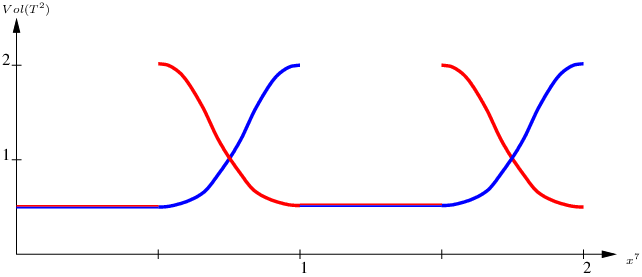
Therefore, it is not too hard to find regions in configuration space that are truly non-geometric. However, in a second step, we must take into account the vacuum selection done by the equations governing string backgrounds. In particular, when we choose an elliptic monodromy, as we did above and we assume that the moduli only depend on the compactification direction , then the moduli will tend to relax to constant values, and in particular, for an elliptic monodromy, the moduli relax to the fixed point of the elliptic monodromy matrix. At these fixed points, then, the elliptic monodromy becomes equivalent to a trivial monodromy (since the modulus is constant). The backgrounds corresponding to these moduli have an enhanced discrete symmetry [6][30]. The discrete symmetry can then be used to (asymmetrically) orbifold the background to make it non-geometric [29].
Note also that once a modulus stabilizes at its fixed point value, it can be interpreted as a modulus with monodromy, or a modulus with trivial monodromy. In other words, those are points in moduli space were a T-fold topology change could occur. The difference between the two interpretations lies in the spectrum of allowed fluctuations. It would be interesting to see whether one can argue for such a T-fold monodromy/topology change transition.
Finally, when we consider constant moduli with hyperbolic and parabolic Scherk-Schwarz ansatz, then we find that these do not provide us with fixed points – the potentials (without gradient terms) exhibit runaway behavior [6].
We can now learn an important lesson from the study of the doubly T-dual to the NS5-brane solution. It provides us with a background with parabolic monodromy, with a modulus that varies over space. Moreover, the solution is stable (and preserves sixteen supercharges). Therefore we are lead to search for new non-geometric backgrounds that allow for a modulus that varies over space, in order to find new non-geometric backgrounds that lie outside the reach of attractive fixed points.
5 A new space-dependent solution
The solutions we studied in detail in the first sections, have a duality twist from the parabolic conjugacy class of . From the analysis of [6], we know that when we reduce the supergravity equations of motion to seven dimensions after reducing on and additionally on a circle with parabolic or hyperbolic duality twists, then there exists no stable constant minimum in the resulting potential.
Since we have a concrete solution, namely the doubly T-dual of NS5-brane solutions, which is stable (since it is supersymmetric) and which has a parabolic duality twist, it is interesting to analyze how we can generalize the analysis of [6] in order to include that type of solution. In doing so, we may learn how to construct interesting solutions of a different type altogether. At the very least, we will find an alternative to the relaxation of the moduli to constant fixed point values.
5.1 The equations of motion in seven dimensions
In this subsection we briefly remind the reader of how dimensional reduction with duality twists proceeds (see e.g. [31, 32]). We concentrate on the part of the eight-dimensional Lagrangian that contains the complex and Kähler moduli describing the geometry of the two-torus on which we compactify. Additionally, we recall that Scherk and Schwarz considered compactifications with fields which depend on the compactified directions [1]. We will reduce the eight-dimensional action further (along the -direction) to seven dimensions using such a Scherk-Schwarz reduction. The dependency of the fields on the direction will be such that it drops out of the eight-dimensional Lagrangian, rendering a further dimensional reduction straightforward. The consistency of the reduction scheme was understood in [1]. Concretely, the ten-dimensional fields do not depend on and directions along the two-torus , and after reducing we have (amongst others) two additional scalar fields, namely the Kähler modulus and the complex structure modulus of the -fiber. In the reduced eight-dimensional Lagrangian they transform under . Next, one Scherk-Schwarz reduces the eight-dimensional fields along the angular direction.
The relevant terms in the eight-dimensional action for the moduli are the invariant coset actions:
| (40) |
The dilatons in eight and ten dimensions are related by the formula
| (41) |
We can rewrite the action in the form
| (42) |
where we take the moduli field to have the form:
| (43) |
We consider a Scherk-Schwarz ansatz for the moduli that guarantees that the dependency will drop out in the Lagrangian:
| (44) |
The unhatted field no longer depends on the angular coordinates . The exponential factors give a monodromy to the moduli of the fiber. Inserting this ansatz into the action (42) we obtain the seven-dimensional reduced action:
| (45) |
with and . In the following we further reduce our ansatz and assume that there is no non-trivial monodromy in the complex structure modulus. We consider only the T-duality transformation and monodromies that act upon the Kähler modulus only. The action is then classically invariant under duality transformations. These act on the matrices and as follows:
| (46) |
where is an matrix. We now recall the action for monodromy matrices in various conjugacy classes of . For the monodromy matrix from the parabolic conjugacy class
we obtain the seven-dimensional action:
| (47) |
For the mass matrix from the elliptic conjugacy class
we obtain
| (48) |
and for the mass matrix from the hyperbolic conjugacy class
| (49) |
we obtain
| (50) |
In the following we further assume that the Kähler modulus is constant along the -directions. In contrast to [6], we allow for a dependence of the moduli on the -direction. As a result, when analyzing solutions to the equations of motion we not only take into account the potential, but also the gradient terms. The equations of motions which we derive from the above actions are
for the parabolic, elliptic and hyperbolic conjugacy classes respectively.
5.2 A space-dependent modulus with parabolic monodromy
We have tuned our ansatz such that the doubly T-dual solution of section 3.1 falls inside the class. We can thus explicitly check on that example the equations of motion, and verify that indeed one finds a spatial dependence of the modulus that gives rise to the desired monodromy. The invariant gradient terms cancel out the (otherwise runaway) potential terms to provide new solutions to the equations of motion. Explicitly, the Kähler modulus of the solution is given by
| (52) |
The monodromy which we read of from its behavior along the angular -direction is
| (53) |
This matches with the Scherk-Schwarz ansatz:
| (54) |
Let’s understand why this provides a solution to the equations of motion. In the background at hand, we have that is constant, and that the metric in is trivial. Moreover such that in the dependent gradient term, the non-trivial mixing with the metric drops out completely. If we then take the real part of the Kähler modulus to be zero and keep the imaginary part to have a generic dependence, than the equation of motion (5.1) simply becomes
| (55) |
The linear function (with ) indeed solves the equation of motion of the seven-dimensional action. We have learned in this example that the gradient terms can compensate for runaway behavior in the potential for a parabolic monodromy. Decoupling of the equations of motion for the Kähler modulus follows from a specific metric ansatz.
5.3 On the existence or not of a geometric T-dual
Both a parabolic and a hyperbolic monodromy matrix do not have a fixed point. They necessarily give rise to non-constant moduli fields. The parabolic monodromy gave rise to a solution that is T-dual to a geometry with flux. One can wonder whether one can find solutions with hyperbolic monodromy, especially in the light of the fact that we argued previously that those cannot be T-dual to geometric backgrounds (when we restrict the action of the T-duality group to be only). Before we attempt to find such a solution, we revisit the analysis of the existence of a geometric dual in the language of the lower-dimensional field theory.
The duality transformation behavior of the moduli field can be used to confirm our discussion about existence/non-existence of the geometric T-dual. We take the working definition that a globally non-geometric background implies that the volume of the -fibration is a non-periodic function of the base-coordinate . For a given globally non-geometric background a test of the existence of the geometric T-dual works as follows.
For a given solution one writes down the matrix
| (56) |
where gives the value of the component and the volume in the given -duality frame. A conjugation of the monodromy matrix by a general -matrix will generate an equivalent background but with a different expression for (see equation (46)). If it possible to find such a -matrix that the new is -independent then a geometric T-dual does exist. One can analyze these conditions generically for the various types of conjugacy classes, and we find the following results:
- •
There is no transformation that transforms away a hyperbolic monodromy along the angular direction.
- •
For the elliptic conjugacy class, the dependence on the angular coordinate is non-trivial unless the modulus is at the fixed point of the monodromy.
- •
For a parabolic monodromy, there is a duality frame in which the modulus is independent of the angular direction .
5.4 A space-dependent modulus with hyperbolic twist
We now turn to finding a solution to the equations of motion (5.1) in the case where we have a hyperbolic duality twist. Equipped with the equation (5.1) we can guess a ten-dimensional solution with duality twist coming from the hyperbolic conjugacy class. When we have vanishing -field (and therefore a purely imaginary Kähler modulus ) the equation (5.1) is solved by a constant . That gives rise to the two-torus geometry coded in
| (57) |
or in other words
| (58) |
Our ansatz for the other metric components is based on the fact that we only expect an dependence of the other fields and metric components, and we moreover are inspired by the relations between these fields in the parabolic solution. Thus, we make the ansatz that only depends on , and that only depends on the coordinate as well. We moreover take . We summarize these proposals in the expression:
| (59) |
We then plug this ansatz directly into the ten-dimensional equations of motion, and find with some effort that they are solved by
| (60) |
with constants.
Let us analyze the solution in slightly more detail. We note that for we obtain the metric and dilaton
| (61) |
which in the new coordinate system reduces to:
| (62) |
A T-duality along the -direction
| (63) |
shows that the metric without monodromy is T-dual to an (almost everywhere) flat background. If we wish to avoid a conical singularity at , we must tune the parameter appropriately.
For a non-zero hyperbolic monodromy, our solution is non-trivial. It cannot be brought into a geometric frame with an duality transformation, and the curvatures are non-trivial. It has a certain domain of validity in which both the curvatures and the string coupling constant are small. The singularity that the original solution exhibits is of a type T-dual to a flat or conical space. It would be good to check the properties of these solutions further, and in particular to study their stability through a fluctuation analysis that properly takes into account the T-fold boundary conditions.
Note also that we have exhibited the solution in a form which is appropriate for hyperbolic monodromies in the full group. It is straightforward to bring it into a form suitable for all -valued twists with . These are of two types of hyperbolic conjugacy classes, namely the generic ones with representatives:
where is an integer with absolute value larger than three, and sporadic conjugacy classes that one can enumerate. Let us give us an example of how to construct a solution with such a monodromy in practice. Consider for example a solution with sporadic monodromy . We will obtain a classically equivalent solution if we set in our solution. Additionally, we can generate infinitely many solutions with this conjugacy class by -conjugation of the monodromy matrix, and in particular there are many frames in which the monodromy is indeed valued. Note that we can also use duality rotations to generate solutions with hyperbolic monodromy and non-trivial NSNS three-form . In summary, we determined a new solution to the equations of motion which has non-trivial varying Kähler modulus that exhibits a hyperbolic monodromy.
To motivate the subsequent subsection, we note that we could turn a background of this form in type IIA/B string theory into a background with hyperbolic monodromy in the complex structure modulus of IIB/A string theory, thus rendering the monodromy geometric. We use a T-duality transformation outside the duality group to achieve this. It should be clear from our previous discussions that the way to avoid such geometrization in a mirror geometry, we need to introduce a non-trivial (say hyperbolic) monodromy for the complex structure as well. Can we find a supergravity solution with a hyperbolic monodromy in both the Kähler and complex structure ?
5.5 Let’s twist again
Indeed, we found a supergravity solution with a non-trivial monodromy in both the Kähler and the complex structure modulus. The underlying reason for the simplicity of the generalization is that the monodromies of both Kähler and complex structure modulus enter the dynamics of the other metric components and the dilaton in a similar fashion. The solution for the metric, dilaton and NSNS two-form is as follows:
| (67) |
From these one learns immediately that the Kähler and complex structure modulus are given by:
| (68) |
Rewriting the moduli fields using the -matrix allows us to identify the type of monodromy for the above solution.
with
| (79) |
For and we have hyperbolic monodromies in both sectors. The solution is genuinely non-geometric under all duality transformations. We can tune the two hyperbolic parameters and use the duality group to construct the solutions for which the hyperbolic monodromies take values in , as we illustrated in the previous subsection.
6 Conclusion
We have given the gravitational backreaction of T-folds T-dual to purely NSNS background. It transpires that twisted tori and T-folds correspond to new types of gravitational singularities which are resolved via T-duality and known resolutions. We extended the analysis to cases with Wilson surfaces and flux on a three-torus localized in one direction. The concept of monodromy domain walls and vortices is useful to describe the microscopic origin of twisted tori. We showed for the importance of including the full backreaction of proposed T-folds in order to judge whether they can be defined in an asymptotically flat string theory.
Moreover, we argued that interesting non-trivial non-geometric backgrounds exist in which we allow the moduli to vary over non-compact space. In fact, the doubly T-dual to a NS5-brane is an example of such a background which is geometrizable. We found a supergravity solution with hyperbolic monodromies which is not equivalent to a geometric one. It will be interesting to further analyze the properties of the solution, and in particular to analyze its stability through a fluctuation analysis that properly takes into account the T-fold boundary conditions.
Thus we showed with an explicit example that one can find regions in the configuration space of second quantized string theory that are non-geometric. It would be good to study these regions further and to estimate to what degree their contributions to a second quantized string theory path integral are important. We expect that they may be of importance for instance in cosmological big crunch big bang scenarios and in string phenomenology.
Acknowledgments
We would like to thank all members of the École Normale Supérieure - Jussieu study group and in particular Costas Bachas, Raphael Benichou and Atish Dabholkar for discussions. Our work was supported in part by the EU under the contract MRTN-CT-2004-005104 and by the ANR (CNRS-USAR) contract 05-BLAN-0079-01.
References
- [1] J. Scherk and J. H. Schwarz, “How To Get Masses From Extra Dimensions,” Nucl. Phys. B 153 (1979) 61.
- [2] E. Alvarez, L. Alvarez-Gaume, J. L. F. Barbon and Y. Lozano, “Some global aspects of duality in string theory,” Nucl. Phys. B 415 (1994) 71 [arXiv:hep-th/9309039].
- [3] C. M. Hull, “Massive string theories from M-theory and F-theory,” JHEP 9811, 027 (1998) [arXiv:hep-th/9811021].
- [4] S. Hellerman, J. McGreevy and B. Williams, “Geometric constructions of nongeometric string theories,” JHEP 0401, 024 (2004) [arXiv:hep-th/0208174].
- [5] S. Kachru, M. B. Schulz, P. K. Tripathy and S. P. Trivedi, “New supersymmetric string compactifications,” JHEP 0303 (2003) 061 [arXiv:hep-th/0211182].
- [6] A. Dabholkar and C. Hull, “Duality twists, orbifolds, and fluxes,” JHEP 0309, 054 (2003) [arXiv:hep-th/0210209].
- [7] C. M. Hull, “A geometry for non-geometric string backgrounds,” JHEP 0510 (2005) 065 [arXiv:hep-th/0406102].
- [8] A. Dabholkar and C. Hull, “Generalised T-duality and non-geometric backgrounds,” JHEP 0605, 009 (2006) [arXiv:hep-th/0512005].
- [9] B. Wecht, “Lectures on Nongeometric Flux Compactifications,” Class. Quant. Grav. 24, S773 (2007) arXiv:0708.3984 [hep-th].
- [10] C. Kounnas, N. Toumbas and J. Troost, “A Wave-function for Stringy Universes,” JHEP 0708 (2007) 018 arXiv:0704.1996 [hep-th].
- [11] P. Bouwknegt, J. Evslin and V. Mathai, “T-duality: Topology change from H-flux,” Commun. Math. Phys. 249, 383 (2004) [arXiv:hep-th/0306062].
- [12] G. Dall’Agata, R. D’Auria and S. Ferrara, “Compactifications on twisted tori with fluxes and free differential algebras,” Phys. Lett. B 619, 149 (2005) [arXiv:hep-th/0503122].
- [13] J. Gray and E. J. Hackett-Jones, “On T-folds, G-structures and supersymmetry,” JHEP 0605, 071 (2006) [arXiv:hep-th/0506092].
- [14] J. Shelton, W. Taylor and B. Wecht, “Nongeometric flux compactifications,” JHEP 0510, 085 (2005) [arXiv:hep-th/0508133].
- [15] V. Mathai and J. Rosenberg, “T-duality for torus bundles with H-fluxes via noncommutative topology. II: The high-dimensional case and the T-duality group,” Adv. Theor. Math. Phys. 10, 123 (2006) [arXiv:hep-th/0508084].
- [16] D. S. Berman, N. B. Copland and D. C. Thompson, “Background Field Equations for the Duality Symmetric String,” Nucl. Phys. B 791 (2008) 175 arXiv:0708.2267 [hep-th].
- [17] D. M. Belov, C. M. Hull and R. Minasian, “T-duality, Gerbes and Loop Spaces,” arXiv:0710.5151 [hep-th].
- [18] C. M. Hull and R. A. Reid-Edwards, “Gauge Symmetry, T-Duality and Doubled Geometry,” arXiv:0711.4818 [hep-th].
- [19] G. Dall’Agata, N. Prezas, H. Samtleben and M. Trigiante, “Gauged Supergravities from Twisted Doubled Tori and Non-Geometric String Backgrounds,” arXiv:0712.1026 [hep-th].
- [20] M. Grana, R. Minasian, M. Petrini and D. Waldram, “T-duality, Generalized Geometry and Non-Geometric Backgrounds,” arXiv:0807.4527 [hep-th].
- [21] C. G. Callan, J. A. Harvey and A. Strominger, “Supersymmetric string solitons,” [arXiv:hep-th/9112030].
- [22] F. Marchesano and W. Schulgin, “Non-geometric fluxes as supergravity backgrounds,” Phys. Rev. D 76, 041901 (2007) arXiv:0704.3272 [hep-th].
- [23] P. M. Cowdall and P. K. Townsend, “Gauged supergravity vacua from intersecting branes,” Phys. Lett. B 429, 281 (1998) [Erratum-ibid. B 434, 458 (1998)] [arXiv:hep-th/9801165].
- [24] T. H. Buscher, “Path Integral Derivation of Quantum Duality in Nonlinear Sigma Models,” Phys. Lett. B 201 (1988) 466.
- [25] A. Giveon, M. Porrati and E. Rabinovici, “Target space duality in string theory,” Phys. Rept. 244 (1994) 77 [arXiv:hep-th/9401139].
- [26] I. Ellwood and A. Hashimoto, “Effective descriptions of branes on non-geometric tori,” JHEP 0612 (2006) 025 [arXiv:hep-th/0607135].
- [27] A. Hanany and A. Zaffaroni, “Issues on orientifolds: On the brane construction of gauge theories with SO(2n) global symmetry,” JHEP 9907 (1999) 009 [arXiv:hep-th/9903242].
- [28] N. J. Hitchin, “Lectures on special Lagrangian submanifolds,” [arXiv:math/9907034].
- [29] K. S. Narain, M. H. Sarmadi and C. Vafa, “Asymmetric Orbifolds,” Nucl. Phys. B 288 (1987) 551.
- [30] A. Flournoy, B. Wecht and B. Williams, “Constructing nongeometric vacua in string theory,” Nucl. Phys. B 706, 127 (2005) [arXiv:hep-th/0404217].
- [31] P. Meessen and T. Ortin, “An Sl(2,Z) multiplet of nine-dimensional type II supergravity theories,” Nucl. Phys. B 541, 195 (1999) [arXiv:hep-th/9806120].
- [32] C. M. Hull, “Gauged D = 9 supergravities and Scherk-Schwarz reduction,” Class. Quant. Grav. 21 (2004) 509 [arXiv:hep-th/0203146].