Growth factor parametrization and modified gravity

The discovery of late time cosmic acceleration [1] challenges our understanding of the standard models of gravity and particle physics. Within the framework of Friedmann-Robertson-Walker cosmology, an exotic energy ingredient with negative pressure, dubbed dark energy, is invoked to explain the observed accelerated expansion of the Universe. One simple candidate of dark energy which is consistent with current observations is the cosmological constant. Because of the many orders of magnitude discrepancy between the theoretical predication and the observation of vacuum energy, other dynamical dark energy models were proposed [2]. By choosing a suitable equation of state $w=p/\rho$ for dark energy, we can recover the observed expansion rate $H(z)$ and the luminosity distance redshift relation $d_{L}(z)$. Current observations are unable to distinguish many different dark energy models which give the same $d_{L}(z)$, and the nature of dark energy is still a mystery. Many parametric and nonparametric model-independent methods were proposed to study the property of dark energy [3, 4, 5, 6, 7, 8, 9, 10, 11, 12, 13, 14, 15, 16, 17].

Bear in mind that the only observable effect of dark energy is through gravitational interaction; it is also possible that the accelerated expansion is caused by modification of gravitation. One example of the alternative approach is provided by the Dvali-Gabadadze-Porrati (DGP) brane-world model [18], in which gravity appears four dimensional at short distances but is modified at large distances. The question one faces is how to distinguish such an alternative approach from the one involving dark energy. One may answer the question by seeking a more accurate observation of the cosmic expansion history, but this will not break the degeneracies between different approaches of explaining the cosmic acceleration. Recently, it was proposed to use the growth rate of large scale in the Universe to distinguish the effect of modified gravity from that of dark energy. While different models give the same late time accelerated expansion, the growth of matter perturbation they produce differ [19]. To linear order of perturbation, at large scales the matter density perturbation $\delta=\delta\rho/\rho$ satisfies the following equation:

where $\rho$ is the matter energy density and $G_{eff}$ denotes the effect of modified gravity. For example, $G_{eff}/G=(4+2\omega)/(3+2\omega)$ for the Brans-Dicke theory [20] and $G_{eff}/G=2(1+2\Omega^{2})/3(1+\Omega^{2})$ for the DGP model [21], the dimensionless matter energy density $\Omega=8\pi G\rho/(3H^{2})$. In terms of the growth factor $f=d\ln\delta/d\ln a$, the matter density perturbation Eq. (1) becomes

where $f^{\prime}=df/d\ln a$. In general, there is no analytical solution to Eq. (2), and we need to solve Eq. (2) numerically; it is very interesting that the solution of the equation can be approximated as $f=\Omega^{\gamma}$ [22, 23, 24, 25] and the growth index $\gamma$ can be obtained for some general models. The approximation was first proposed by Peebles for the matter dominated universe as $f(z=0)=\Omega^{0.6}_{0}$ [22]; then a more accurate approximation, $f(z=0)=\Omega^{4/7}_{0}$, for the same model was derived in [23, 24]. For the Universe with a cosmological constant, the approximation $f(z=0)=\Omega^{0.6}_{0}+\Omega_{\Lambda 0}(1+\Omega_{0}/2)/70$ can be made [26]. For a dynamical dark energy model with slowly varying $w$ and zero curvature, the approximation $f(z)=\Omega(z)^{\gamma}$ was given in [25]. For the DGP model, $\gamma=11/16$ [27]. Therefore, instead of looking for the growth factor by numerically solving Eq. (2), the growth index $\gamma$ may be used as the signature of modified gravity and dark energy models. It was found that $\gamma=0.55+0.05[1+w(z=1)]$ with $w>-1$ and $\gamma=0.55+0.02[1+w(z=1)]$ with $w<-1$ for the dynamical dark energy model in flat space [28, 27]. Recently, the use of the growth rate of matter perturbation in addition to the expansion history of the Universe to differentiate dark energy models and modified gravity attracted much attention [29, 30, 31, 32, 33, 34, 35, 36, 37, 38, 39, 40, 41, 42, 43, 44].

The dependence of $\gamma$ on the equation of state $w$ has received much attention in the literature; we discuss the dependence of $\gamma$ on $\Omega$ and $\Omega_{0}$ for a more accurate approximation in this paper. We discuss a more accurate approximation for the dark energy model with constant $w$ in Sec. II. Then we discuss the DGP model in Sec. III. In Sec. IV, we apply the Union compilation of type Ia supernovae (SNe) data [45], the baryon acoustic oscillation (BAO) measurement from the Sloan Digital Sky Survey (SDSS) [46], the shift parameter measured from the Wilkinson Microwave Anisotropy Probe 5 yr data (WMAP5) [47], the Hubble parameter data $H(z)$ [48, 49], and the growth factor data $f(z)$ [42, 44, 50] to constrain the models. We also use the growth factor data alone to find out the constraint on the growth index $\gamma$. We conclude the paper in Sec. V.

We first review the derivation of $\gamma$ given in [25]. For the flat dark energy model with constant equation of state $w$, we have

The energy conservation equation tells us that

Substituting Eqs. (3) and (4) into Eq. (2), we get

Plugging $f=\Omega^{\gamma}$ into Eq. (5), we get

Expanding Eq. (6) around $\Omega=1$, to the first order of $(1-\Omega)$, we get [25]

In order to see how well the approximation $\Omega^{\gamma}$ fits the growth factor $f$, we need to solve Eq. (6) numerically with the expression of $\Omega$. The dimensionless matter density is

Since $\gamma$ does not change very much, we first use $\gamma=\gamma_{\infty}=3(1-w)/(5-6w)$ to approximate the growth factor. For convenience, we choose $\Omega_{0}=0.27$, and the result is shown in Fig. 1.

From Fig. 1, we see that $\Omega^{\gamma_{\infty}}$ approximates $f$ better than 2%.

For the $\Lambda$CDM model, $w=-1$, so the growth index becomes

and

For the $\Lambda$CDM model, the matter density is

Substituting Eq. (11) into Eq. (6) and solving the equation numerically, we compare the numerical result $f$ with the analytical approximation $\Omega^{\gamma}$. The results are shown in Figs. 2 and 3. Since $\gamma_{1}$ is very small, $\gamma$ does not change much, and we can take the approximation $\gamma=\gamma_{\infty}$. In Fig. 2, we compare $\Omega^{\gamma_{\infty}}$ with $f$ for different values of $\Omega_{0}$. From Fig. 2, we see that $\Omega^{\gamma_{\infty}}$ approximates $f$ very well; the smaller $\Omega_{0}$, the larger the error. When the Universe deviates farther from the matter dominated era, the error becomes larger. For $\Omega_{0}=0.2$, the approximation overestimates $f$ by only 2%, or $\gamma_{\infty}$ underestimates $\gamma$. To get a better approximation, we expand to the first order of $(1-\Omega)$ and use $\gamma=\gamma_{\infty}+\gamma_{1}(1-\Omega)$. In Fig. 3, we plot the relative difference between $\Omega^{\gamma}$ and $f$. From Fig. 3, we see that using $\gamma=\gamma_{\infty}+\gamma_{1}(1-\Omega)$ approximates the growth factor much better; now the error is only 0.6% for $\Omega_{0}=0.2$.

For the flat DGP model, we have

The Friedmann equation tells us that

The energy conservation equation tells us that

The matter energy density is given by

Substituting Eqs. (12), (13) and (14) into Eq. (2), we get

Plugging $f=\Omega^{\gamma}$ into Eq. (16), we get

Expanding Eq. (17) around $\Omega=1$, to the first order of $(1-\Omega)$, we get

So $\gamma_{\infty}=11/16$ and $\gamma_{1}=7/5632$. The change of $\gamma$ is very small because $\gamma_{1}$ is very small; we first approximate $\gamma$ by $\gamma_{\infty}$ and the result is shown in Fig. 4. From Fig 4, we see that the error becomes larger when the Universe deviates farther from the matter domination. When $\Omega_{0}=0.2$, $\Omega^{\gamma_{\infty}}$ underestimates $f$ by 4.6%. So the growth factor is overestimated. If we use the first order approximation, the error becomes larger because $\gamma_{1}>0$. Linder and Cahn give the approximation [27]

Again, to the first order approximation of $(1-\Omega)$, the error becomes larger than that with $\gamma_{\infty}$. In [43], the author found the approximation

In this approximation, the correction to $\gamma_{\infty}$ is too big because $\gamma_{1}$ is too large even though the sign is correct. To get better than 1% approximation, we first assume $\gamma$ is a constant and solve Eq. (17) at $\Omega=\Omega_{0}$ to get $\gamma_{0}$; we then approximate $\gamma_{1}=(\gamma_{0}-\gamma_{\infty})/2(1-\Omega_{0})$. The values of $\gamma_{0}$ and $\gamma_{1}$ for different $\Omega_{0}$ are listed in table 1. The difference between $\Omega^{\gamma}$ with $\gamma=\gamma_{\infty}+\gamma_{1}(1-\Omega)$ and $f$ is shown in Fig. 5. As promised, the error is under 1%.

Now we use the observational data to fit the dark energy model with constant $w$ and the DGP model. The parameters in the models are determined by minimizing $\chi^{2}=\chi^{2}_{sn}+\chi^{2}_{a}+\chi^{2}_{r}+\chi^{2}_{h}+\chi^{2}_{f}$. For the SNe data, we use the reduced Union compilation of 307 SNe [45]. The SNe compilation includes the Supernova Legacy Survey [51] and the ESSENCE Survey [52, 53], the older observed SNe data, and the extended dataset of distant SNe observed with the Hubble space telescope. To fit the SNe data, we define

where the extinction-corrected distance modulus $\mu(z)=5\log_{10}[d_{L}(z)/{\rm Mpc}]+25$, $\sigma_{i}$ is the total uncertainty in the SNe data, and the luminosity distance is

The dimensionless Hubble parameter $E(z)=H(z)/H_{0}=[\Omega_{0}(1+z)^{3}+(1-\Omega_{0})(1+z)^{3(1+w)}]^{1/2}$ for the dark energy model with constant $w$ and $E(z)=[\Omega_{0}(1+z)^{3}+(1-\Omega_{0})^{2}/4]^{1/2}+(1-\Omega_{0})/2$ for the DGP model. The nuisance parameter $H_{0}$ is marginalized over using a flat prior.

To use the BAO measurement from the SDSS data, we define $\chi^{2}_{a}=(A-0.469(0.96/0.98)^{-0.35})^{2}/0.017^{2}$, where the distance parameter [46, 47]

To use the shift parameter measured from the WMAP5 data, we define $\chi^{2}_{r}=(\mathcal{R}-1.715)^{2}/0.021^{2}$, where the shift parameter [47]

Simon, Verde, and Jimenez obtained the Hubble parameter $H(z)$ at nine different redshifts from the differential ages of passively evolving galaxies [48]. Recently, the authors in [49] obtained $H(z=0.24)=83.2\pm 2.1$ and $H(z=0.43)=90.3\pm 2.5$ by taking the BAO scale as a standard ruler in the radial direction. To use these 11 $H(z)$ data, we define

where $\sigma_{hi}$ is the $1\sigma$ uncertainty in the $H(z)$ data. We also add the prior $H_{0}=72\pm 8$ km/s/Mpc given by Freedman et al. [54].

For the growth factor data, we define

where $\sigma_{fi}$ is the $1\sigma$ uncertainty in the $f(z)$ data. For reference, we compile the available data [42, 44, 50] in Table 2. The data are obtained from the measurement of the redshift distortion parameter $\beta=f/b$, where the bias factor $b$ measures how closely galaxies trace the mass density field. Note that some of the measured redshift distortion parameter $\beta$ is obtained by fitting $\Omega^{0.6}$ with $\Omega$ given by the $\Lambda$CDM model, and some analyses tried to account for extra distortions due to the geometric Alcock-Paczynski effect [50]. With these caveats in mind, it is still worthwhile to apply the data to fit the models. As discussed in the previous sections, we can use $\gamma=\gamma_{\infty}$ within the accuracy of a few percent. For the $\Lambda$CDM model, we use $\gamma=6/11$ and $\Omega$ given by Eq. (11). For the DGP model, we use $\gamma=11/16$ and $\Omega$ given by Eq. (15).

By fitting the dark energy model with constant $w$ to the combined data, we get $\chi^{2}=325.17$, $\Omega_{0}=0.272^{+0.023}_{-0.022}$, and $w=-0.97\pm 0.09$. The $1\sigma$, $2\sigma$, and $3\sigma$ contours of $\Omega_{0}$ and $w$ are shown in Fig. 6. From Fig. 6, we see that the $\Lambda$CDM model is consistent with the current observation. By fitting the $\Lambda$CDM model to the combined data, we get $\chi^{2}=325.48$ and $\Omega_{0}=0.273\pm 0.015$. By fitting the DGP model to the combined data, we get $\chi^{2}=350.12$ and $\Omega_{0}=0.278\pm 0.015$.

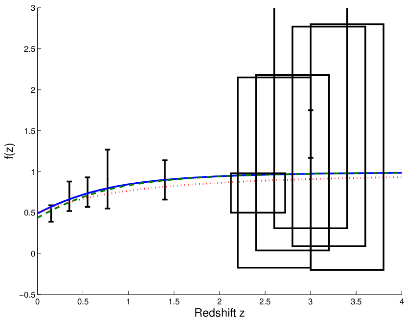
If we fit $\Omega^{\gamma}$ to the growth factor data $f(z)$ alone, we can get a constraint on the growth index $\gamma$. For the $\Lambda$CDM model with the best fit value $\Omega_{0}=0.273$, we find that $\chi^{2}=4.55$ and $\gamma_{\Lambda}=0.64^{+0.17}_{-0.15}$. The theoretical value $\gamma_{\infty}=6/11=0.55$ is consistent with the observation at the $1\sigma$ level. For the DGP model with the best fit value $\Omega_{0}=0.278$, we find $\chi^{2}=5.68$ and $\gamma_{DGP}=0.55^{+0.14}_{-0.13}$ which is barely consistent with the theoretical value $\gamma_{\infty}=11/16=0.6875$ at the $1\sigma$ level. The best fit curves $\Omega^{\gamma}$ and the observational data are shown in Fig. 7.

The simple analytical formulas $\Omega^{\gamma}$ can be used to approximate the growth rate $f$. The value of $\gamma$ provides useful information about the dark energy model and the modification of gravity. For the dark energy model within general relativity, $\gamma\approx 0.55$. For the DGP model, $\gamma=0.6875$. If the accuracy of the growth factor data is in the range of a few percent, we can use a constant $\gamma_{\infty}$ to approximate $f$. For example, $\gamma_{\infty}=3(1-w)/(5-6w)$ for constant $w$ [25], $\gamma_{\infty}=0.55+0.05[1+w(z=1)]$ for dynamical models [28], and $\gamma_{\infty}=11/16$ for the DGP model. The value of $\gamma_{\infty}$ is obtained by approximating the differential equation of $f$ around $\Omega=1$. This approximation is reasonably good at high redshift ($z\gtrsim 1$) when $\Omega\approx 1$. However, at lower redshift the dark energy or the effect of modified gravity starts to dominate and $\Omega$ deviates from 1; we expect the approximation to break down. Therefore, to get a better than 1% fit, the $\Omega$ dependence of $\gamma$ needs to be considered. We show that $\gamma=\gamma_{\infty}+\gamma_{1}(1-\Omega)$ can approximate $f$ to better than 1%. The value of $\gamma_{1}$ is very small compared with $\gamma_{\infty}$ and usually depends on the value of $\Omega_{0}$. For the $\Lambda$CDM model, $\gamma_{1}=15/1331$. For the DGP model, we give a prescription of how to find $\gamma_{1}$; the values of $\gamma_{1}$ are listed in Table 1 for some values of $\Omega_{0}$.

To distinguish different dark energy models and modified gravity, we use the observational data to fit the models. Fitting the combined SNe, SDSS, WMAP5, $H(z)$, and $f(z)$ data to the dark energy model with constant $w$, we find that $\chi^{2}=325.17$, $\Omega_{0}=0.272^{+0.023}_{-0.022}$, and $w=-0.97\pm 0.09$. For the $\Lambda$CDM model, we find that $\chi^{2}=325.48$ and $\Omega_{0}=0.273\pm 0.015$. For the DGP model, we find that $\chi^{2}=350.12$ and $\Omega_{0}=0.278\pm 0.015$. The results suggest that the data strongly disfavor the DGP model. If we fit the SNe data alone to the DGP model, we get $\chi^{2}=313.27$ and $\Omega_{0}=0.186$. This result is consistent with the results in [62, 63, 64, 65, 66, 67, 68]. If the same data were fitted to the $\Lambda$CDM model, we would get $\chi^{2}=312.18$. If we fit the $\Lambda$CDM model to the combined SNe and $H(z)$ data, we get $\chi^{2}=319.45$. For the DGP model, we get $\chi^{2}=321.31$ and $\Omega_{0}=0.194$. These results show that both the $\Lambda$CDM model and the DGP model give almost the same expansion rate. If we fit the $\Lambda$CDM model to the combined SNe, $H(z)$, and $f(z)$ data, we get $\chi^{2}=324.53$. For the DGP model, we get $\chi^{2}=331.53$ and $\Omega_{0}=0.207$. With the addition of $f(z)$ data to the expansion data, the DGP model is readily distinguishable from the $\Lambda$CDM model. As mentioned above, the best fit value of $\Omega_{0}$ in the DGP model tends to be lower, i.e., $\Omega_{0}\approx 0.2$, when we fit the model to the SNe, $H(z)$, and $f(z)$ data. On the other hand, we get $\chi^{2}=1.4$ and $\Omega_{0}=0.33$ if we fit the model to the distance parameter $A$ and the shift parameter $\mathcal{R}$. If the two sets of data are combined together, $\Omega_{0}$ takes the value in the middle and we get a large value of $\chi^{2}$. When we fit the models to the combined SNe, the distance parameter $A$, the shift parameter $\mathcal{R}$, and $H(z)$ data, we get $\Omega_{0}=0.274$ and $\chi^{2}=320.6$ for the $\Lambda$CDM model and $\Omega_{0}=0.275$ and $\chi^{2}=343.5$ for the DGP model. This result is consistent with the analysis by Song et al [62]. In [62], they found that the flat DGP model is excluded at about $3\sigma$ by the combined SNe, 3 yr WMAP, and Hubble constant data.

The observational data of $f(z)$ can be used to provide information on the growth index $\gamma$ and the modified gravity. As discussed above, $\gamma$ is almost a constant; we can use $\Omega^{\gamma}$ with a constant $\gamma$ to approximate $f(z)$. For the $\Lambda$CDM model, we find that $\gamma_{\Lambda}=0.64^{+0.17}_{-0.15}$, which is consistent with the theoretical value 0.55. This result is also consistent with that in [44, 42]. For the DGP model, we find that $\gamma_{DGP}=0.55^{+0.14}_{-0.13}$. The theoretical value $\gamma=0.6875$ lies on the upper limit of the $1\sigma$ error. From Fig. 7, we see that the growth rates for the DGP model and the $\Lambda$CDM model are distinguishable even with the best fitting values of $\gamma$. If the theoretical values of $\gamma$ are used, the difference will be larger. The approximation of $\Omega^{\gamma}$ to $f$ is good for theories with $f\leq 1$ and $\Omega\leq 1$. If the observational data for $f(z)$ are larger than 1 at high redshift ($z\gtrsim 1$), then the approximation $\Omega^{\gamma}$ is broken and the effect of modified gravity is explicit. For the Brans-Dicke theory, during the matter domination, $\Omega=(3\omega+4)(2\omega+3)/6(1+\omega)^{2}\geq 1$ and $f=(2+\omega)/(1+\omega)\geq 1$ [42]; here $\omega$ is the Brans-Dicke constant. In this case, modification of the approximation is needed. This will be discussed in future work. In conclusion, more precise future data on $f(z)$ along with the SNe data will differentiate dark energy models from modified gravity.