Correlation functions of the energy-momentum tensor
in SU(2) gauge theory at finite temperature
Abstract
We calculate correlation functions of the energy-momentum tensor in the vicinity of the deconfinement phase transition of (3+1)-dimensional SU(2) gauge theory and discuss their critical behavior in the vicinity of the second order deconfinement transition. We show that correlation functions of the trace of the energy momentum tensor diverge uniformly at the critical point in proportion to the specific heat singularity. Correlation functions of the pressure, on the other hand, stay finite at the critical point. We discuss the consequences of these findings for the analysis of transport coefficients, in particular the bulk viscosity, in the vicinity of a second order phase transition point.
pacs
11.15.Ha, 11.10.Wx, 12.38Gc, 12.38.MhI Introduction
Experimental evidence for rapid thermalization of the dense matter created in heavy ion collisions at RHIC [1] provided strong motivation for a new look at the non-perturbative structure of the quark gluon plasma (QGP). The rapid thermalization of the QGP has been related to the smallness of the shear viscosity in the plasma phase [2], which may come close to the theoretical lower bound established for the ratio of shear viscosity to entropy density [3]. This gave rise to the interpretation of the quark gluon plasma above but close to the transition temperature as a strongly interacting medium that has properties of an almost perfect liquid.
These experimental findings also renewed the interest in determining transport properties of gauge theories through the calculation of correlation functions of the energy-momentum tensor on the lattice. This is by far not a straightforward calculation and requires a careful analysis of the low frequency structure of the spectral representation of these correlation functions [4]. Nonetheless progress has been made through high statistics calculations in SU(3) gauge theories [5, 6, 7].
Recently it has been argued that close to the transition from low temperature hadronic matter to the plasma phase of QCD bulk viscosity might play a much more important role than shear viscosity [8]; bulk viscosity has been related to a temperature derivative of the trace of the energy-momentum tensor. The latter does diverge at a second order critical point [9] and thus would force bulk viscosity to diverge too. This argument is based on a sum rule derived for correlation functions of the energy-momentum tensor in Minkowski space [8]. However, as noted recently [10], in Euclidean space the correlation function of the trace of the energy-momentum tensor picks up an additional constant contribution corresponding to an exact -function at zero frequency in the spectral representation of this correlator. This contribution, in fact, cancels the leading singular behavior of the correlation function and thus makes the relation between transport coefficients and properties of bulk thermodynamic observables more subtle.
In the following we will provide evidence for the presence of a contribution to the correlation function of the trace of energy-momentum tensor that is constant in Euclidean time but temperature dependent. We show that the temperature dependence of this contribution scales like the specific heat and thus dominates the singular behavior of this correlation function in the vicinity of . These findings also explain the inconsistency observed in the parametric dependence of bulk viscosity derived in high temperature perturbation theory and through the sum rule analysis [11].
The singular behavior of bulk viscosity in the vicinity of a critical point has long been known in statistical physics [12, 13]. In particular, the divergence of bulk viscosity at the critical point of the liquid gas transition has been analyzed extensively [14]. In this case the divergence of bulk viscosity () has been related to the critical behavior of the 3-dimensional Ising model [13, 15, 16], which is in the universality class for the critical point of the liquid-gas phase transition. It has been argued that the divergence of is strong and, in fact, almost quadratic in the inverse reduced temperature, . The singular behavior, , with denoting static critical exponents of the 3-d Ising model and being a dynamical exponent characterizing the equilibration of density fluctuations, goes along with a strong divergence of the relaxation time for density fluctuations, . Their ratio, , however, is proportional to the inverse of the specific heat and thus vanishes slowly at the critical point.
While numerous numerical studies have confirmed that the critical behavior of bulk thermodynamics in -dimensional gauge theories is indeed controlled by -dimensional universality classes corresponding to the global symmetry of the relevant order parameter, little is known about the relation between dynamic properties and the related critical exponents [17]. The SU(2) gauge theory with its second order deconfinement phase transition seems to be an ideal model to explore critical behavior of dynamical properties, e.g. transport coefficients. The SU(2) gauge theory at finite temperature incorporates all the basic features one expects to be relevant for deconfinement in QCD. Moreover, it has a second order phase transition which belongs to the universality class of the 3-dimensional Ising model. It thus will allow to analyze in how far dynamic universal properties known for the Ising universality class are relevant for transport properties in a quantum field theory. It also may give insight into transport properties in the vicinity of the chiral critical point in QCD that may exist at non-zero baryon number density and also would belong to the Ising universality class [18]. In the vicinity of the SU(2) deconfinement phase transition a lot of information exists about the critical behavior of bulk thermodynamics that can be related to the critical behavior of correlation functions of the energy-momentum tensor. This will help to gain experience with lattice calculations of the bulk viscosity in pure gauge theories.
In this paper we will establish relations between the critical behavior of bulk thermodynamic observables in the vicinity of the SU(2) deconfinement transition and properties of correlation functions of the energy-momentum tensor. In particular, we will analyze the Euclidean correlation functions of the trace of the energy-momentum tensor and compare it to critical behavior of the specific heat. We present evidence that the strength of the divergence of this correlation function at is independent of Euclidean time and is controlled by the universal structure of the divergence of the specific heat at a critical point belonging to the 3-dimensional Ising universality class. In the next section we review the calculation of bulk thermodynamic observables in SU(2) gauge theory [19] and present some new results on the diagonal components of the energy-momentum tensor, i.e. energy density and pressure, in the vicinity of the deconfinement transition temperature. In Section III we introduce local operators for energy density and pressure and discuss basic properties of their finite temperature Euclidean time correlation functions at vanishing momentum. Section IV is devoted to a discussion of critical behavior extracted from correlation functions of the trace anomaly and presents a calculation of the pressure-pressure correlator. We analyze consequences for the determination of bulk viscosity from these correlation functions in Section V. Finally, we conclude in Section VI.
II Thermodynamics of SU(2) gauge theories on the lattice
As preparation for the analysis of correlation functions of diagonal elements of the energy-momentum tensor we want to discuss here the calculation of the relevant bulk thermodynamic observables, energy density () and pressure (), on the lattice. In order to analyze Euclidean space-time correlation functions of , or the trace of the energy-momentum tensor, , one obviously needs to use an approach to bulk thermodynamics that allows to define local operators for energy density and pressure. We will call this approach, which in fact was the basis for the original formulation of bulk thermodynamics on the lattice [21], the differential formalism. It is in contrast to the so-called integral method which nowadays is most commonly used in lattice calculations to extract energy density and pressure from the trace anomaly [22]. The differential formalism has not been used recently in studies of bulk thermodynamic observables as it is more involved and requires additional non-perturbative calculations of derivatives of the bare gauge couplings with respect to the anisotropy parameter, , that controls the spatial () and temporal () lattice spacings [23]. Having control over the anisotropy is needed to derive thermodynamic quantities as function of temperature, , and volume, through appropriate partial derivatives with respect to and [21], although numerical calculations will generally be performed on isotropic lattice (). In particular, for the study of the singular behavior of the energy density in the vicinity of the SU(2) deconfinement transition this approach has been used successfully [19]. In this context also the necessary derivatives of the gauge coupling with respect to had been analyzed in detail. We will follow this analysis here closely.
II.1 The differential formalism
We start from the partition function for a gauge theory at finite temperature, which we write in standard lattice notation [24],
| (1) |
with
| (2) |
Here labels the discrete set of space-time points on a four-dimensional hypercubic lattice of size .
In the standard Wilson discretization scheme the local gauge action in the -hyperplane is expressed in terms of plaquette variables , with link variables . We write the action in terms of contributions arising only from entirely space-like plaquettes () and space-time like plaquettes (),
| , | |||||
| , | (3) |
We also introduce as the average of space-like and time-like plaquettes evaluated on a symmetric () lattice, i.e. for .
From the logarithm of the partition function one obtains pressure and energy density as derivatives with respect to and , respectively [21],
| (4) | |||||
| (5) |
Here and are given in terms of derivatives of the gauge coupling, , with respect to the anisotropy at [21, 23]. Their sum is constraint by the -function,
| (6) |
With these relations for and it is straightforward to obtain also the trace of the energy-momentum tensor and the entropy density,
| (7) | |||||
| (8) |
We note that these particular combinations of energy density and pressure are proportional to simple sums and differences of space-like and time-like plaquette expectation values. They only require common multiplicative renormalizations for and . Extracting or directly, however, involves different renormalization factors for space-like and time-like plaquette expectation values. For this reason it is straightforward to analyze correlation functions of local densities of the entropy or trace anomaly. We note that in the vicinity of the SU(2) deconfinement transition the dominant singular behavior of as well as is controlled by the energy density. We will show later that in the vicinity of the pressure is an order of magnitude smaller than the energy density. When one combines and to extract the pressure it thus requires good knowledge of the renormalization factors and in order to eliminate the dominant energy contributions and arrive at a proper definition for a local operator for the pressure. This is a prerequisite for the analysis of pressure-pressure correlation functions and, as will become clear later, this becomes of importance for studies of transport coefficients, e.g. the bulk viscosity, in the vicinity of .
II.2 Critical energy density and pressure
As an application of the differential formalism reviewed above we have performed a finite size scaling analysis of the critical energy density and the pressure at the deconfinement transition temperature of the SU(2) gauge theory. This extends earlier studies of the critical energy density performed in Ref. [19] to larger lattices and yields, for the first time, a determination of the pressure at the critical point.
The deconfinement transition of the SU(2) gauge theory in (3+1)-dimensions is in the same universality class as the 3-dimensional Ising model. Its critical behavior is well understood and has been confirmed in various finite size scaling studies. On a lattice of size energy density and pressure at the critical point are expected to scale as
| (9) | |||||
| (10) |
Here and denote the critical exponents of the 3-dimensional Ising universality class, controlling the divergence of the specific heat and the correlation length, respectively11 1 Note that the leading finite volume correction that arises from the singular contribution to the pressure is inverse proportional to the volume as it is the case also for the leading corrections to regular terms. This is due to a hyper-scaling relation, with ..


We have analyzed the scaling behavior of energy density and pressure on lattices with temporal extent and for various spatial lattice sizes; covering the range for , and for and for . For these values of the infinite volume critical couplings are known quite precisely [25, 26, 27]. We have listed them in Table 1. At these values of the gauge coupling also the anisotropy coefficients and have been determined previously [19].
We have calculated pressure, energy density, entropy density and trace anomaly on lattices of temporal extent and for various spatial lattice sizes at the critical couplings given in Table 1. Data for the vacuum subtraction needed for all observables but the entropy density have been obtained through simulations on a lattice. The number of configurations analyzed ranges from on our smaller lattices to on the large lattices. For our calculations on and lattices we have used a standard heat-bath/over-relaxation algorithm. For calculations on the larger lattices it became possible to use also a two-level algorithm [20] which turned out to be more efficient for the analysis of correlation functions. Autocorrelation times in the transition region range from on the small lattices to about on the largest lattices.
In Fig. 1 we show results for the volume dependence of various bulk thermodynamic observables. It clearly can be seen that the scaling behaviour of the pressure is different from that of the other three observables. Moreover, it is apparent that the pressure is more than an order of magnitude smaller than any of the observables that contain contributions of the energy density. This shows that the finite size scaling behavior of and is dominated by the non-analytic behavior of the energy density and thus is expected to be controlled by the same ansatz as for the energy density given in Eq. 10. We also note that cut-off effects seem to be small already for lattices with temporal extent and that the volume dependence starts being controlled by the scaling variable . This may be expected as bulk thermodynamics in the vicinity of is dominated by low frequency modes for which the underlying lattice cut-off becomes unimportant.
To check consistency with the scaling behavior of the Ising universality class we have fitted the data for the energy on the lattice for all to the ansatz given in Eq. 10 with a free scaling exponent . This fit yields which is in good agreement with the value in the 3-dimensional Ising universality class, [29]. Fits to the finite volume corrections for the pressure yield an exponent in good agreement with the expected hyper-scaling relation .
To extract the asymptotic, infinite volume values for the critical energy density and the pressure we then used the ansätze given in Eqs. 9 and 10 with fixed scaling exponents and , respectively. Results for and for as well as infinite volume extrapolated values are summarized in Table 1; results for the critical energy density are consistent with those of Ref. [21] but have a statistical error that is an order of magnitude smaller. Comparison of the results with those for suggest that the remaining cut-off dependence is small.
| 4 | 2.29895(10) | 0.3303(9) | 0.0240(2) | 0.2872(5) | 0.0242(3) |
| 6 | 2.4265(30) | 0.3015(27) | 0.0136(8) | 0.2722(31) | 0.0135(8) |
| 8 | 2.5115(40) | 0.3158(42) | 0.0107(26) | – | 0.0107(15) |
III Correlation functions of the energy-momentum tensor
Within the differential framework for bulk thermodynamics on the lattice, reviewed in the previous section, it is straightforward to define local operators for the energy density and pressure, as well as the entropy density and the trace of the energy momentum tensor. Using and as introduced in Eq. 3 one obtains from Eqs. 4, 5 and Eqs. 7, 8 local operators for pressure, energy and entropy density as well as the trace anomaly, e.g.
| (11) |
for the trace anomaly and similar for other observables. The local plaquette variables, have been defined in Eq. 3. We will denote this particular choice of local expressions for plaquette variables in the following as discretization scheme 1. However, when considering correlation functions in Euclidean time, one may want to account for the effect that time-like plaquettes connect two different time-slices in a lattice and should be connected to a Euclidean time that is displaced from that of space-like plaquettes. This ambiguity arises because gauge fields are introduced on links of the lattice and the field strength tensor thus is spread at least over a domain of the size of an elementary plaquette. This effects introduce additional discretization errors, i.e. errors that are of the same order as the discretization errors that exist anyhow in the definition of the Euclidean action or the energy-momentum tensor used in our calculations. They, of course, will disappear in the continuum limit. Nonetheless, comparing different discretization schemes will allow to estimate the magnitude of systematic effects. We therefore have introduced two other discretization schemes which symmetrize the contribution of space-like plaquettes relative to a time-like plaquette or vice verse,
scheme 2: ,
scheme 3: .
Note that there is no need for a local definition for which enters the definition of . is evaluated at zero temperature and is a constant, identical at all space-time points. We furthermore introduce zero-momentum projected operators and their fluctuations,
| (12) |
Correlation functions are then obtained as thermal averages over products of fluctuation operators, i.e. we consider connected correlation functions,
| (13) |
Due to the periodic boundary conditions in Euclidean time points in the hyperplane at are identical to those at . In the following we also will discuss properties of the midpoint-subtracted correlation functions,
| (14) |
We used the three discretization schemes introduced above for diagonal components of the energy-momentum tensor to analyze the cut-off dependence of correlation functions. In Fig. 2(left) we show results for correlation functions of the trace of the energy momentum tensor, and the energy, . These correlators have been evaluated on lattices with the largest temporal extent, , used in this study, and at the largest Euclidean time separation possible at finite temperature, i.e. the midpoint of the temporal direction . It is apparent from these figures that cut-off effects in are only of the order of 10%; within the current errors different discretization schemes yield consistent results on the lattices. For , however, discretization errors are large even on the largest lattices.
In the right hand part of Fig. 2 we show the energy-energy and energy-pressure correlation functions as function of Euclidean time, , evaluated at the critical temperature. As has been pointed out in Ref. [10] these correlation functions will, in the continuum limit, be independent of Euclidean time as the energy operator is time independent,
| (15) |
At finite lattice spacing, however, this is not yet the case. It is apparent from Fig. 2(right) that the influence of a finite lattice cut-off is more severe at shorter distances, and correlation functions thus show a significant dependence on Euclidean time.


As a consequence, the simple relation between midpoint-subtracted correlation functions of and pressure-pressure correlators,
| (16) | |||||
| (17) |
which holds in the continuum limit, is violated by corrections at finite lattice spacing. The left hand side of Eq. 16 as well as the various components of the right hand side are shown in Fig. 3 for and . In the continuum limit the differences and should vanish and should be equal to . This is clearly not the case for finite values of the lattice cut-off.

IV Correlation functions and critical behavior
Fortunately, the cut-off dependence discussed in the previous section is not crucial for the analysis of critical behavior as it arises from short-distance effects. Close to , however, the correlation length is large and thermal effects are not very sensitive to the underlying cut-off. The cut-off dependence thus is part of the smooth regular background that contributes to . This is apparent from the weak temperature dependence of the differences shown in Fig. 3. Moreover, we find that correlators calculated in the three discretization schemes show a similar temperature dependence and differ, at fixed only by an almost temperature independent shift.
IV.1 Correlation function of
We will discuss here the temperature dependence of correlation functions of at vanishing momentum, i.e. we calculate as introduced in Eq. 13. This correlation function is the sum of three contributions corresponding to energy-energy, pressure-pressure and energy-pressure correlations, respectively,
| (18) |
As discussed above in the continuum limit the entire -dependence of is expected to arise from the pressure-pressure correlations, while close to the dominant temperature dependence will arise from the energy-energy correlator, which through the fluctuation-dissipation theorem, is proportional to the specific heat,
| (19) |
Close to the deconfinement transition we therefore expect that will show critical behavior that coincides with that of the specific heat in a 3-dimensional Ising model,
| (20) |
Here is the specific heat critical exponent and is the correction to scaling exponent which characterizes the leading non-analytic scaling correction. Like also the exponent is universal. For the gauge theory in (3+1)-dimensions, which we are analyzing here, the relevant universality class is that of the 3-dimensional Ising model. In this case and [29] which also has been verified in lattice calculations [19].
At non-zero lattice spacing the direct relation between correlation functions involving the energy operator and temperature derivatives of any observable is violated by cut-off effects. Nonetheless we expect that these are small in the vicinity of a second order phase transition. One thus may expect that at least the singular behavior of correlation functions that involve correlations with the energy operator will be independent of Euclidean time. Will analyze the critical behavior of in the next two subsections and show explicitly that the leading singular behavior indeed is independent of Euclidean time.
IV.2 Finite size scaling of at the critical point
We have calculated the correlation function close to the deconfinement transition point of the SU(2) gauge theory. In most of our simulation we use lattices of size with . This gives us information on the correlation function at two non-zero values of Euclidean time, i.e. at and at the midpoint . Most of our simulations have been performed at temperatures close to the phase transition where the correlation length becomes large. This required calculations on large spatial lattices in order to eliminate finite volume effects. We used spatial lattice sizes with aspect ratios varying from ( lattices) up to values as large as 32 ( lattices). This large aspect ratio made it possible to perform calculations at temperatures in the proximity of without being affected by large finite volume effects. We checked that for all temperature values, except for calculations performed directly at , the thermodynamic limit has been reached within our numerical accuracy. To reach the statistical accuracy needed for our scaling tests close to the critical point, where fluctuations are large, we have generated a large number of gauge field configurations ranging from on our smaller lattices to on the large lattices.
As mentioned in Section II.B the location of the critical point is quite well known for lattices with temporal extent [25]. The relation between gauge coupling and temperature has been determined in the vicinity of non-perturbatively from calculations of the transition temperature on lattices of temporal size [19]. We use these results to determine the reduced temperature .
In various studies of the critical behavior of bulk thermodynamics of the (3+1)-dimensional SU(2) gauge theory it has been established that this gauge theory belongs to the universality class of the 3-dimensional Ising model. In our analysis of the critical behavior of correlation functions of the energy-momentum tensor we use established results on the critical exponents , and as well as the universal ratio of the specific heat amplitudes, . These parameters are summarized in Table 2.
| 0.110(1) | 0.6301(4) | 0.84(4) | 0.54(1) |


In Fig. 4(left) we show results for the correlation function calculated at the midpoint, , on lattices with temporal extent and for various spatial lattice sizes. As can be seen at all temperatures except, of course, at the dependence on the spatial volume is well under control. The peak at the pseudo-critical point close to rises only slowly with increasing size of the volume as the specific heat exponent is quite small. The right hand part of Fig. 4 shows the volume dependence of the correlation function evaluated at on lattices with temporal extent at the two non-zero distances accessible in this case. At we have fitted the volume dependence of to a finite size scaling ansatz, which includes the leading singular behavior of the specific heat and a correction-to-scaling term,
| (21) |
Here , , are fit parameters, which all might depend on Euclidean time. We performed fits for the two non-zero Euclidean time separations reachable on lattices with temporal extent , i.e. and . In the fits we make use of the known Ising exponents , and which are given in Table 2. This ansatz gives excellent finite size scaling fits for both data sets shown in Fig. 4(right). This confirms that the critical behavior is controlled by the exponents of the 3-dimensional Ising model. When performing fits of the data sets at distance and separately, we observe that the amplitudes and agree within errors. This also is apparent from the fact that the data at can be shifted on top of the data at by a independent constant (open squares in Fig. 4(right)). We then performed simultaneous fits of both data sets, still allowing for different amplitudes at both distances. From this combined fit we find that and . The fit results22 2 Note that the coefficients of the correction-to-scaling term, , are negative. Although these amplitudes are non-universal it has been noted previously that for the 3-dimensional Ising model on various lattice geometries this correction term comes out to be negative [30]. are summarized in Table 3, which also includes the coefficients extracted from an equally good combined fit of both data sets obtained requiring the same coefficients , and for the two Euclidean distances.
| free | 1/4 | 16.3(2.1) | -0.59(19) | -1.9(1.4) | 21.5(5.7) | -150(53) | 9.2(1.2) | -2.4(1.0) | 26.3(2.7) |
| fit | 1/2 | 16.4(2.2) | -0.76(18) | -2.2(1.5) | 3.7(3.4) | -95(32) | 9.1(1.2) | -2.4(0.9) | 8.4(2.9) |
| combined | 1/4 | 16.5(1.3) | -0.74(10) | -2.12(86) | 21.8(2.1) | -143(20) | 9.15(73) | -2.39(59) | 26.4(1.9) |
| fit | 1/2 | 3.8(1.9) | -87(18) | 8.3(1.7) |
The analysis presented above establishes that the correlation function of the trace of the energy-momentum tensor shows the expected universal singular structure of the specific heat in a 3-dimensional Ising model. In the vicinity of the singular contributions to are found to be independent of Euclidean time. We have performed corresponding analyzes for and which are consistent with these findings, however statistical errors are larger in these cases.
The analysis presented above confirms that the correlation function contains a constant contribution that arises from low frequency modes that lead to the singular behavior of the energy-energy correlation function at . In the continuum limit this constant will reflect the -independence of the correlators and .
IV.3 Critical behavior of in the vicinity of
In the previous subsection we established through a finite size scaling analysis at that the singular terms in are independent of Euclidean time. We will show here that this is also the case at temperatures in the vicinity of at which the universal scaling behavior allows to separate the long-distance singular behavior of from regular contributions.

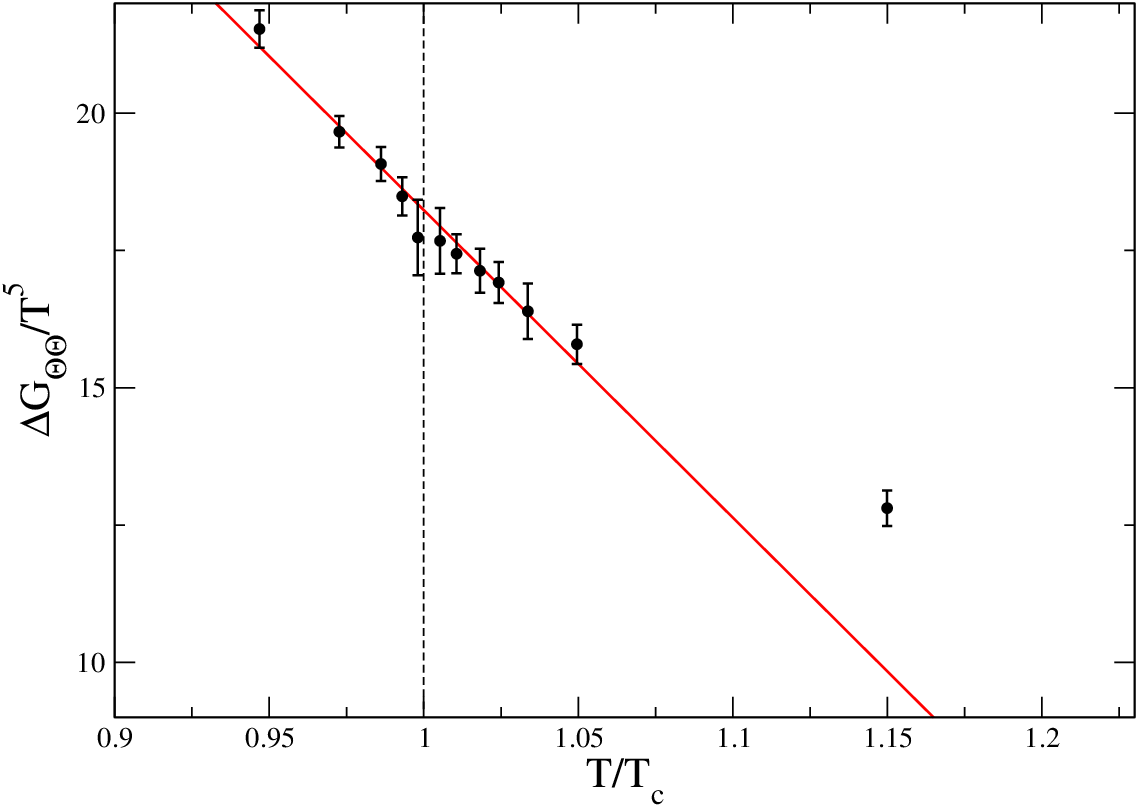
In Fig. 5 (left) we show infinite volume extrapolated results for at two distances, and . Here we left out the data at . At both distances increases rapidly when approaches ; above the correlation function changes by a factor 2 in the temperature interval .
In the vicinity of we expect that the data are well described by the scaling ansatz,
| (22) |
where , , , are free parameters, which again all may depend on Euclidean time; and , and are the known Ising exponents given in Table 2. We again have performed fits for the two data sets at and separately as well as simultaneously. The ansatz given in Eq. 22 gives good fits in the interval . As expected the parameters extracted for and , are consistent with the constant terms obtained from the finite size scaling analysis at .
Again we find that within errors the fit parameters and are independent of ; a combined fit of and with common amplitudes and also gives a . The resulting fit parameters are also given in Table 3.
We thus conclude that in the vicinity of the critical point of the SU(2) gauge theory the temperature dependence of the correlation function of the energy-momentum tensor reflects the singular behavior of the specific heat of 3-dimensional Ising model. More striking may be the fact that the amplitudes for the singular terms are to a good approximation independent of . However, as discussed above this is consistent with the expected -independence of the energy-energy correlation function [10].
In order to eliminate the leading singular behavior from it thus suffices to consider differences of the correlation function evaluated for different Euclidean time separations, e.g.
| (23) |
Fig. 5(right) shows that this difference indeed stays finite at . However, as shown in Fig. 2, at non-zero value of the lattice spacing does not yet coincide with as it will in the continuum limit.
We finally show in Fig. 6 the temperature dependence of the different correlation functions, , contributing to . As can be seen the entire strong temperature dependence of in the vicinity of indeed arises from . All other correlators show only a weak temperature dependence in the vicinity of . In particular, we find that the pressure-pressure correlation function stays finite at and varies little in its vicinity. As will be discussed in the next section this has immediate consequences for the determination of the bulk viscosity from correlation functions of the energy-momentum tensor.

V Bulk viscosity and relaxation time scale
Correlation functions of the energy-momentum tensor are widely used to gain information on transport coefficients. The spectral representation of these Euclidean-time correlation functions and their relation to real-time Kubo formulas allow, in principle, to extract transport coefficients from the zero frequency limit of spectral functions [4]. We want to discuss here some consequences for the calculation of transport coefficients, in particular the bulk viscosity, that can be drawn from the analysis of correlation functions presented in the previous sections.
The bulk viscosity can be extracted from the spectral representation of pressure-pressure correlation functions [4],
| (24) |
where
| (25) |
and is the spectral density at vanishing momentum. Making use of the definition of transport coefficients via the Kubo-formulas it is readily seen that the bulk viscosity is related to the low frequency limit of this spectral function [28],
| (26) |
From Eq. 18 it is obvious that this can also be obtained from a spectral analysis of the correlator of the trace of the energy-momentum tensor. However, as we have verified explicitly in the previous sections this correlation function receives a constant contribution from correlation functions containing the energy operator. This constant term is reflected in zero frequency contribution to , i.e. a -function at vanishing frequencies,
| (27) |
with
| (28) |
As the bulk viscosity is obtained from the spectral function in the limit of vanishing frequency one should eliminate the contribution arising from . This can, of course, easily be done by analyzing the subtracted correlation function introduced in Eq. 23. From Fig. 5(right) we know that this correlation function will stay finite at . Its spectral representation is given by
| (29) |
The low frequency part of the spectral function, , is expected to be linear, the slope being proportional to the bulk viscosity. The rise of the spectral functions ends at a characteristic frequency , which is identified as a characteristic relaxation time scale, , for density fluctuations. Of course, will be temperature dependent and, in fact, is expected to vanish at a second order phase transition point where fluctuations grow and relaxation times will diverge.
We may split the spectral function into a low frequency part and a large frequency part, . The low frequency behavior of the spectral function may be modeled by a Breit-Wigner ansatz,
| (30) |
With this we can write the low frequency contribution to the pressure correlator, , as
| (31) | |||||
Here we have assumed in the second equality that becomes small in the vicinity of and an expansion in thus is appropriate. Similarly we can obtain the low frequency contribution to . Both correlation functions have the same functional dependence on Euclidean time for . It is this region, where one can hope that the low frequency part of the spectral function dominates the -dependence of the correlation functions and thus will allow a determination of transport properties.
From Eq. 31 we find that the low frequency part of the spectral function, which is proportional to bulk viscosity, contributes a term proportional to to the value of the correlation function at the midpoint, . As discussed in the introduction, universality arguments given for the scaling of the bulk viscosity in the vicinity of a critical point in the Ising universality class suggest, however, that the ratio of bulk viscosity and relaxation time, , vanishes as the inverse of the specific heat, i.e. it is expected to be proportional to the velocity of sound. In the vicinity of the correlation function thus is dominated by contributions from the large frequency, regular part of the spectral function. The sensitivity to bulk viscosity also is small away from the midpoint where contributions from the low frequency part of the spectral function are proportional to . To separate this contribution from the large frequency contributions it would be necessary to become sensitive to the characteristic logarithmic dependence on Euclidean time that arises from the low frequency part of the spectral function.
VI Conclusions
We have shown that the correlation function of the trace of the energy-momentum tensor, , diverges at the critical point of the finite temperature SU(2) gauge theory in (3+1)-dimensions. The divergence is controlled by the critical exponent of the 3-dimensional Ising model that also controls the divergence of the specific heat. Furthermore, we have shown that becomes independent of Euclidean time at the critical point, which indicates that its spectral representation receives a contribution from a -function at zero frequency. This confirms the observations made in Ref. [10].
To get direct access to the bulk viscosity and the characteristic frequency that controls the relaxation time for density fluctuations will require much more detailed studies of the dependence of correlation functions on Euclidean time. In fact, we conclude that a determination of bulk viscosity from correlation functions of the energy-momentum tensor is not possible without a simultaneous determination of the relevant relaxation time scale.
Acknowledgments
We thank Harvey Meyer, Dimitri Kharzeev and Kirill Tuchin for helpful discussions. This work has been supported by the contract DE-AC02-98CH10886 with the U.S. Department of Energy. Numerical simulations have been performed on the BlueGene/L at the New York Center for Computational Science (NYCCS).
References
- [1]
I. Arsene et al. [BRAHMS Collaboration], Nucl. Phys. A 757, 1
(2005);
B.B. Back et al. [PHOBOS Collaboration], Nucl. Phys. A 757, 28 (2005);
J. Adams et al. [STAR Collaboration], Nucl. Phys. A 757, 102 (2005);
K. Adcox et al. [PHENIX Collaboration], Nucl. Phys. A 757, 184 (2005). - [2] D. Teaney, Phys. Rev. C 69, 034913 (2003).
- [3] P. Kovtun, D. T. Son and A. O. Starinets, Phys. Rev. Lett. 94, 111601 (2005).
- [4] F. Karsch and H. W. Wyld, Phys. Rev. D 35, 2518 (1987).
- [5] A. Nakamura and S. Sakai, Phys. Rev. Lett. 94, 072305 (2005).
- [6] H. B. Meyer, Phys. Rev. D 76, 101701 (2007).
- [7] H. B. Meyer, Phys. Rev. Lett. 100, 162001 (2008).
- [8] D. Kharzeev and K. Tuchin, arXiv:0705.4280 [hep-ph].
- [9] F. Karsch, D. Kharzeev and K. Tuchin, Phys. Lett. B 663, 217 (2008).
- [10] H. B. Meyer, arXiv:0805.4567 [hep-lat].
- [11] G. D. Moore and O. Saremi, arXiv:0805.4201 [hep-ph].
- [12] M. Fixman, J. Chem. Phys. 36, 310 (1961).
- [13] K. Kawasaki, Phys. Rev. 150, 291 (1966).
- [14] P.C. Hohenberg and B.I. Halperin, Rev. Mod. Phys. 49, 435 (1977).
- [15] L.P. Kadanoff and J. Swift, Phys. Rev. bf 166, 89 (1968).
- [16] A. Onuki, J. Phys. Soc. Jap. 66, 511 (1997) and Phys. Rev. E 55, 403 (1997).
- [17] K. Okano, L. Schulke and B. Zheng, Phys. Rev. D 57, 1411 (1998).
- [18] M. A. Stephanov, K. Rajagopal and E. V. Shuryak, Phys. Rev. Lett. 81, 4816 (1998).
- [19] J. Engels, F. Karsch and K. Redlich, Nucl. Phys. B 435, 295 (1995).
- [20] M. Luscher and P. Weisz, JHEP 0109, 010 (2001)
- [21] J. Engels, F. Karsch, H. Satz and I. Montvay, Nucl. Phys. B 205, 545 (1982).
- [22] J. Engels, J. Fingberg, F. Karsch, D. Miller and M. Weber, Phys. Lett. B 252, 625 (1990).
- [23] F. Karsch, Nucl. Phys. B 205 (1982) 285.
- [24] F. Karsch, Lect. Notes Phys. 583, 209 (2002).
- [25] J. Engels and T. Scheideler, Nucl. Phys. B 539, 557 (1999).
- [26] J. Engels, J. Fingberg and D. E. Miller, Nucl. Phys. B 387, 501 (1992).
- [27] J. Fingberg, U. Heller and F. Karsch, Nucl. Phys. B 392, 493 (1993).
- [28] S. Jeon and L. G. Yaffe, Phys. Rev. D 53, 5799 (1996).
- [29] A. Pelissetto and E. Vicari, Phys. Rept. 368, 549 (2002).
- [30] A.J. Liu and M.E. Fisher, J. Stat. Phys. 58, 431 (1990).