Symplectic approach to quantum constraints

Practical implementations of quantum algorithms in quantum information technology can be hampered by constraints. The formulation of a tractable theory of the properties of constrained unitary motions is therefore of interest and importance. This paper provides a framework for dealing with certain classes of constrained quantum motion, for which differential equations governing the constrained dynamics can be obtained explicitly. The results are applied to constrain unitary motions to algebraic subspaces of quantum state spaces.

The structure and the findings of the paper can be summarised as follows. We begin by reviewing the Hamiltonian formulation of standard quantum mechanics. This highly effective way of looking at quantum mechanics has been investigated by a number of authors (see [1, 2, 3, 4, 5, 6, 7, 8, 9] and references cited therein). We demonstrate the existence of a particularly simple choice of canonically conjugate coordinates $(\{q_{i}\},\{p_{i}\})$ for the space of pure quantum states with the property that the Schrödinger equation can be written in Hamiltonian form:

$\displaystyle\dot{q}_{i}=\frac{\partial H(q,p)}{\partial p_{i}}\quad{\rm and}\quad\dot{p}_{i}=-\frac{\partial H(q,p)}{\partial q_{i}}.$

(1)

The coordinates $(\{q_{i}\},\{p_{i}\})$ appearing here are defined by the expansion coefficients of the normalised state vector $|\psi\rangle$ of a non-degenerate $n$-level system in terms of the energy eigenstates $\{|E_{i}\rangle\}_{i=1,2,\ldots,n}$ according to the scheme

$\displaystyle|\psi\rangle=\sum_{i=1}^{n-1}\surd{p_{i}}\mbox{$\rm e$}^{-{\rm i}q_{i}}|E_{i}\rangle+\left(1-\sum_{i=1}^{n-1}p_{i}\right)^{\frac{1}{2}}|E_{n}\rangle,$

(2)

where the function

$\displaystyle H(q,p)=\frac{\langle\psi|{\hat{H}}|\psi\rangle}{\langle\psi|\psi\rangle}$

(3)

is given by the expectation of the Hamiltonian operator in the state defined by (2). We choose the overall phase such that the coefficient of the $n$th energy eigenstate $|E_{n}\rangle$ is real. Since in the energy basis we have

$${\hat{H}}=\sum_{i=1}^{n}E_{i}|E_{i}\rangle\langle E_{i}|,$$

(4)

it follows that the Hamiltonian function is given by

$\displaystyle H(q,p)=E_{n}+\sum_{i=1}^{n-1}\omega_{i}p_{i},$

(5)

where $\omega_{i}=E_{i}-E_{n}$. Note that $H(q,p)$ is independent of $\{q_{i}\}$ and is linear in $\{p_{i}\}$. Substitution of (5) in (1) shows that the solution to the Schrödinger equation

$$\mbox{$\rm i$}\frac{\partial}{\partial t}|\psi_{t}\rangle={\hat{H}}|\psi_{t}\rangle$$

(6)

is given in terms of the canonical coordinates by

$\displaystyle q_{i}(t)=q_{i}(0)+\omega_{i}t\quad{\rm and}\quad p_{i}(t)=p_{i}(0),$

(7)

which should also be evident from (2). For simplicity we shall consider Hamiltonians having nondegenerate eigenvalues, although the formalism can be applied to degenerate systems by use of the Lüders projection postulate [10]. Specifically, the state $|\psi\rangle$ is still expressible in the form (2), but we make the replacement $n\to d$, where $d<n$ is the number of distinct energy eigenvalues, and $|E_{i}\rangle=\hat{\Pi}_{i}|\psi\rangle$, where $\hat{\Pi}_{i}$ is the projection operator onto the eigenspace associated with the eigenvalue $E_{i}$, given by

$\displaystyle\hat{\Pi}_{i}=\sum_{j=1}^{d_{i}}|E_{i},j\rangle\langle E_{i},j|.$

(8)

Here $d_{i}$ is the dimension of the Hilbert subspace associated with the eigenvalue $E_{i}$, and $|E_{i},j\rangle$ $(j=1,\ldots,d_{i})$ constitute an orthonormal basis for that subspace. The Hamiltonian for a general system is hence given by

$\displaystyle\hat{H}=\sum_{i=1}^{d}E_{i}\hat{\Pi}_{i},$

(9)

and one sees that the form of (5) remains unchanged, except that $n$ is replaced by $d$, and $H(q,p)$ is independent of the remaining phase space degrees of freedom.

The objective of this paper is to introduce a framework for treating certain classes of constrained unitary motion. Our approach is aligned closely with that of Dirac’s theory of constraints in classical mechanics [11, 12]. The idea that Dirac’s methodology might be applied to investigate constrained quantum motion was proposed recently by Burić [13] to determine the dynamics of a pair of spin-$\textstyle\frac{1}{2}$ particles constrained to a special surface of product states containing all of the energy eigenstates. An alternative approach to quantum constraints is considered in [14].

An elementary way of enforcing the constraints is to introduce Lagrange multipliers. In some circumstances the Lagrange multipliers can be determined explicitly and eliminated from the equations of motion. In this paper we shall be considering such cases. Several examples are investigated, including one for which the motion of a pair of spin-$\textstyle\frac{1}{2}$ particles is constrained to the hypersurface of disentangled states.

Constrained unitary motions are in general nonunitary, and correspond to nonlinear evolutions. However, unlike the general nonlinear dynamics of the Mielnik-Kibble-Weinberg (MKW) framework [3, 4, 15], the nonlinearities resulting from the class of constraints considered in the present investigation are of a milder form. That is, while in the MKW theory one considers a general Hamiltonian $H(q,p)$ that is distinct from (5), in the present context the ‘linear’ Hamiltonian (5) remains unchanged, and the nonlinearity arises from a modification of the symplectic structure, or equivalently on account of the nonlinearity of the constraint surface.

In the first example we consider a system of two spin-$\frac{1}{2}$ particles. The constraint surface is defined by the product space of a pair of two-dimensional Hilbert spaces, and we assume that the product space contains the energy eigenstates. An initial state that lies on the constraint surface is thus obliged to remain on this surface. We shall obtain the trajectories of the unitary evolutions subject to this constraint. The analysis can be extended and applied to $n$ spin-$\textstyle\frac{1}{2}$ particles constrained to a special product space containing the energy eigenstates. We find that this constraint is satisfied under unitary evolution without constraint if the spectrum of the trace-free part of the Hamiltonian takes the form $\{E_{i}\}=\{e_{1},e_{2},\cdots,e_{n/2},-e_{n/2},-e_{n/2-1},\cdots,-e_{1}\}$, where $n$ is the number of eigenstates of the system. For a generic Hamiltonian we derive and solve the constrained equations of motion explicitly in the case of two and three spin-$\frac{1}{2}$ particle systems. Surprisingly, the resulting dynamics turn out to be quasi-unitary in the sense that the amplitudes $\{p_{i}\}$ remain constant while the relative phases $\{q_{i}\}$ evolve linearly. This property appears to be generic even for systems with more particles. We then consider the motion of two spin-$\frac{1}{2}$ particles constrained to remain on the quadric corresponding to the subspace of disentangled states.

Let us now begin with a summary of the Hamiltonian formulation of quantum mechanics. We consider a complex Hilbert space ${\mathcal{H}}^{n}$ of dimension $n$, a typical element of which is denoted $|\psi\rangle$. If ${\hat{F}}$ represents an observable, its expectation with respect to $|\psi\rangle$ is $F=\langle\psi|{\hat{F}}|\psi\rangle/\langle\psi|\psi\rangle$, which is invariant under the transformation $|\psi\rangle\to\lambda|\psi\rangle$, $\lambda\in{\mathds{C}}-\{0\}$. The vector $|\psi\rangle$ thus carries a redundant complex degree of freedom. We therefore construct the space of rays through the origin of ${\mathcal{H}}^{n}$ by the identification $|\psi\rangle\sim\lambda|\psi\rangle$. The result is the projective Hilbert space ${\mathcal{P}}^{n-1}$ of dimension $n-1$. We can view ${\mathcal{P}}^{n-1}$ as a real even-dimensional manifold $\Gamma$, and let $\{x^{a}\}_{a=1,2,\ldots,2n-2}$ denote a typical point of $\Gamma$. One distinguishing feature of $\Gamma$ is that it is equipped with a symplectic structure $\Omega^{ab}(=-\Omega^{ba})$ such that the Schrödinger equation (6) can be expressed in the Hamiltonian form

$\displaystyle\dot{x}^{a}=\Omega^{ab}\nabla_{b}H.$

(10)

Here the function $H(x)=\langle\psi(x)|{\hat{H}}|\psi(x)\rangle/\langle\psi(x)|\psi(x)\rangle$ denotes the expectation of the operator ${\hat{H}}$ in the pure state $|\psi(x)\rangle$ corresponding to the point $x\in\Gamma$. One can regard $\Gamma$ as a bona fide quantum analogue of the phase space in classical mechanics.

Now suppose that we have a family of constraints on the motion of the system in $\Gamma$ expressed in the form

$\displaystyle\Phi^{\alpha}(x)=0,$

(11)

where $\alpha=1,2,\ldots,N$. There are two different types of constraints that arise naturally in the quantum context, corresponding to what one might call ‘algebraic’ and ‘real’ constraints. In the algebraic case the motion is confined to an algebraic submanifold (or possibly a complex algebraic subvariety) of the original quantum state space ${\mathcal{P}}^{n-1}$. As a consequence, the constraint submanifold is of even real dimension—for which it follows that the number of constraints $N$ is even in this case. This paper is primarily concerned with the algebraic case. Typical examples would include the situations where the constraint manifold ${\mathfrak{M}}$ was an algebraic curve in ${\mathcal{P}}^{2}$ (such as a conic or a elliptic cubic curve), or an algebraic curve in ${\mathcal{P}}^{3}$ (such as a twisted cubic curve or an elliptic quartic curve), or an algebraic surface in ${\mathcal{P}}^{3}$ (such as a quadric surface, or a cubic surface). The equations given by (11) then define ${\mathfrak{M}}$ locally.

The other situation that is natural to consider in quantum theory is the case where the constraints are of the form

$\displaystyle\Phi^{\alpha}(x)=\frac{\langle\psi(x)|{\hat{F}}^{\alpha}|\psi(x)\rangle}{\langle\psi(x)|\psi(x)\rangle}-f^{\alpha},$

(12)

where $\{{\hat{F}}^{\alpha}\}_{\alpha=1,\ldots,N}$ denotes a collection of observables, $\{f^{\alpha}\}_{\alpha=1,\ldots,N}$ is a set of real numbers, and $N$ need not be even. We shall consider the ‘real’ case elsewhere.

In the algebraic case, the constraints can be enforced by the introduction of Lagrange multipliers $\{\lambda_{\alpha}\}_{\alpha=1,2,\ldots,N}$. Using the usual summation convention, the constrained equations of motion are

$$\dot{x}^{a}=\Omega^{ab}\nabla_{b}H+\lambda_{\alpha}\Omega^{ab}\nabla_{b}\Phi^{\alpha}.$$

(13)

To determine the Lagrange multipliers we analyse the relation $\dot{\Phi}^{\alpha}(x)=0$. From the chain rule we have $\dot{\Phi}^{\alpha}=\dot{x}^{a}\nabla_{a}\Phi^{\alpha}=0$. Substituting (13) in here, we find

$$\Omega^{ab}\nabla_{a}\Phi^{\alpha}\nabla_{b}H+\lambda_{\beta}\Omega^{ab}\nabla_{a}\Phi^{\alpha}\nabla_{b}\Phi^{\beta}=0.$$

(14)

To solve (14) for $\lambda_{\alpha}$ let us define

$$\omega^{\alpha\beta}=\Omega^{ab}\nabla_{a}\Phi^{\alpha}\nabla_{b}\Phi^{\beta}.$$

(15)

In the case of real constraints, for which $\{\Phi^{\alpha}\}$ corresponds to a family of observables, $\omega^{\alpha\beta}$ is the commutator of the observables $\Phi^{\alpha}$ and $\Phi^{\beta}$. We note that since $\Omega^{ab}=-\Omega^{ba}$ we have $\omega^{\alpha\beta}=-\omega^{\beta\alpha}$.

If the matrix $\omega^{\alpha\beta}$ is nonsingular, then we can invert it. In that case, writing $\omega_{\alpha\beta}$ for the inverse of $\omega^{\alpha\beta}$ so $\omega^{\alpha\beta}\omega_{\beta\gamma}=\delta^{\alpha}_{\phantom{\alpha}\gamma}$, we can solve (14) for $\{\lambda_{\alpha}\}$ to obtain

$$\lambda_{\alpha}=\omega_{\beta\alpha}\Omega^{ab}\nabla_{a}\Phi^{\beta}\nabla_{b}H.$$

(16)

Substituting this in the right side of (13) yields

$$\dot{x}^{a}=\Omega^{ab}\nabla_{b}H+\omega_{\beta\alpha}\Omega^{cd}\nabla_{c}\Phi^{\beta}\nabla_{d}H\Omega^{ab}\nabla_{b}\Phi^{\alpha}.$$

(17)

This can be simplified further by rearrangement of indices, after which we deduce that

$$\dot{x}^{a}={\tilde{\Omega}}^{ab}\nabla_{b}H,$$

(18)

where ${\tilde{\Omega}}^{ab}=\Omega^{ab}+\Lambda^{ab}$ and

$$\Lambda^{ab}=\Omega^{ac}\Omega^{bd}\omega_{\gamma\delta}\nabla_{c}\Phi^{\gamma}\nabla_{d}\Phi^{\delta}.$$

(19)

An important point to note is that $\Lambda^{ab}$ is by construction antisymmetric. Therefore, ${\tilde{\Omega}}^{ab}$ defines a modified symplectic structure. The constrained equation of motion (18) thus takes on a form identical to (10), with the same Hamiltonian, but with the modified symplectic structure.

The modified symplectic structure can be interpreted as playing the role of an induced symplectic structure on the constraint surface $\Phi=0$. To see this we transvect $\tilde{\Omega}^{ab}$ with the vector $\nabla_{a}\Phi^{\alpha}$ normal to the constraint surface to obtain

$\displaystyle\tilde{\Omega}^{ab}\nabla_{b}\Phi^{\alpha}=\Omega^{ab}\nabla_{b}\Phi^{\alpha}+\Omega^{ac}\Omega^{bd}\omega_{\gamma\delta}\nabla_{c}\Phi^{\gamma}\nabla_{d}\Phi^{\delta}\nabla_{b}\Phi^{\alpha}.$

(20)

Using the antisymmetry of $\Omega^{ab}$ and the definition (15) we find

$\displaystyle\Omega^{bd}\nabla_{d}\Phi^{\delta}\nabla_{b}\Phi^{\alpha}=-\omega^{\delta\alpha}.$

(21)

Hence from $\omega_{\gamma\delta}\omega^{\delta\alpha}=\delta_{\gamma}^{\alpha}$ we deduce that

$\displaystyle\tilde{\Omega}^{ab}\nabla_{b}\Phi^{\alpha}=0$

(22)

for all $\alpha$. Therefore, $\tilde{\Omega}^{ab}$ annihilates all vectors normal to the constraint surface, and hence induces a symplectic structure on the constraint surface.

Our procedure for dealing with a constrained unitary motion can be summarised as follows: (i) find a suitable choice of $2n-2$ real coordinates for representing the generic pure state $|\psi\rangle$; (ii) calculate the symplectic structure $\Omega^{ab}$ in that coordinate system so that the unitary evolution is represented in the Hamiltonian form (10); (iii) express the constraints (11) in terms of the given choice of coordinates; (iv) assuming that the constraints are such that the matrix $\omega^{\alpha\beta}$ of (15) is invertible, calculate $\Lambda^{ab}$ according to (19) and substitute the result into (18). In this way, dynamical equations for constrained unitary motion can be obtained, and one is left with the problem of solving a system of coupled differential equations.

As we have indicated, there is a particular choice of coordinates on the space of pure states for which the analysis can be simplified in the form defined in (2), which might appropriately be called an ‘action-angle’ parametrisation (cf. [16]). In terms of these coordinates $\Omega^{ab}$ is given by

$\displaystyle\Omega^{ab}=\left(\begin{array}[]{cc}{\mathds{O}}&{\mathds{1}}\\ -{\mathds{1}}&{\mathds{O}}\end{array}\right),$

where ${\mathds{O}}$ and ${\mathds{1}}$ denote the $(n-1)\times(n-1)$ null matrix and identity matrix. As a consequence, the dynamical equations (10) take the form (1).

It is worth noting that while in classical mechanics phase space coordinates correspond to observables, in quantum mechanics only half of the phase space coordinates correspond to observables. Specifically, if we write ${\hat{\Pi}}_{i}=|E_{i}\rangle\langle E_{i}|$ for the observable corresponding to the projection operator onto the $i$th normalised energy eigenstate, then $p_{i}=\langle\psi|{\hat{\Pi}}_{i}|\psi\rangle$. Therefore the coordinates $\{p_{i}\}_{i=1,2,\ldots,n-1}$ constitute a commuting family of observables. The conjugate variables $\{q_{i}\}_{i=1,2,\ldots,n-1}$, correspond to the relative phases, and do not represent observables in the conventional sense.

Example 1. We now apply the formalism to specific examples. The first example is a system consisting of a pair of spin-$\frac{1}{2}$ particles. For a generic Hamiltonian, we shall impose the constraint that under the dynamics the initial state of the system remains on a quadratic surface ${\mathcal{Q}}={\mathcal{P}}^{1}\times{\mathcal{P}}^{1}\subset\Gamma$ that contains the energy eigenstates. Such a constraint implies that the quantum state can be represented as a product state with respect to some choice of basis elements. The Hilbert space is four dimensional and a generic state can be expressed in the form

$\displaystyle|\psi\rangle=\surd{p_{1}}\mbox{$\rm e$}^{-{\rm i}q_{1}}|E_{1}\rangle+\surd{p_{2}}\mbox{$\rm e$}^{-{\rm i}q_{2}}|E_{2}\rangle+\surd{p_{3}}\mbox{$\rm e$}^{-{\rm i}q_{3}}|E_{3}\rangle+(1-p_{1}-p_{2}-p_{3})^{1/2}|E_{4}\rangle.$

(26)

The space of pure states is the three-dimensional space ${\mathcal{P}}^{3}$, in which sits the two-dimensional product space ${\mathcal{Q}}$. The constraint for the state to remain on ${\mathcal{Q}}$ is therefore of an algebraic type—that is, $|\psi\rangle$ must lie on the algebraic subspace ${\mathcal{Q}}$. If we write $\{\psi_{i}\}_{i=1,\ldots,4}$ for the coordinates of the Hilbert space vector $|\psi\rangle=(\psi_{1},\psi_{2},\psi_{3},\psi_{4})$, then a necessary and sufficient condition for $|\psi\rangle$ to lie on ${\mathcal{Q}}$ is $\psi_{1}\psi_{4}=\psi_{2}\psi_{3}$ [9]. Expressing the real and the imaginary parts of this condition in terms of the coordinates chosen in (26) we find that the constraint equations are given by

$\displaystyle\begin{array}[]{l}\sqrt{p_{1}p_{4}}\,\cos q_{1}-\sqrt{p_{2}p_{3}}\,\cos(q_{2}+q_{3})=0\\ \sqrt{p_{1}p_{4}}\,\sin q_{1}-\sqrt{p_{2}p_{3}}\,\sin(q_{2}+q_{3})=0,\end{array}$

where for brevity we have written $p_{4}=1-p_{1}-p_{2}-p_{3}$. If we divide the first equation in (Symplectic approach to quantum constraints) by $\sqrt{p_{2}p_{3}}\,\cos q_{1}$ and the second by $\sqrt{p_{2}p_{3}}\,\sin q_{1}$, and compare the results, we find that the constraint equations can be made separable:

$\displaystyle\begin{array}[]{l}\Phi^{1}=q_{1}-q_{2}-q_{3}\\ \Phi^{2}=p_{1}(1-p_{1}-p_{2}-p_{3})-p_{2}p_{3}.\end{array}$

Before we proceed to derive the constrained dynamical equations, we address the following question: What is the condition on ${\hat{H}}$ that will ensure that under unitary evolution an initial state that lies on ${\mathcal{Q}}$ remains on ${\mathcal{Q}}$? The answer is obtained by substituting the solution (7) of the unitary motion into the constraints (Symplectic approach to quantum constraints). We thus obtain the condition that $\omega_{1}=\omega_{2}+\omega_{3}$. Translated into the eigenvalues of ${\hat{H}}$ this condition is $E_{1}-E_{2}=E_{3}-E_{4}$. It follows that the trace-free part of the Hamiltonian must have the eigenvalue structure $\{e_{1},e_{2},-e_{2},-e_{1}\}$.

We now turn to the general case for which $E_{1}-E_{2}\neq E_{3}-E_{4}$. As a consequence of the separable decomposition (Symplectic approach to quantum constraints), the matrix $\omega^{\alpha\beta}$ and its inverse $\omega_{\alpha\beta}$ are remarkably simple in this example:

$\displaystyle\omega^{\alpha\beta}=\left(\begin{array}[]{cc}{\mathds{O}}&{\mathds{1}}\\ -{\mathds{1}}&{\mathds{O}}\end{array}\right)\quad{\rm and}\quad\omega_{\alpha\beta}=\left(\begin{array}[]{cc}{\mathds{O}}&-{\mathds{1}}\\ {\mathds{1}}&{\mathds{O}}\end{array}\right).$

It follows that

$\displaystyle\Lambda^{ab}=\left(\begin{array}[]{cc}{\mathds{O}}&{\mathds{A}}\\ -{\mathds{A}}&{\mathds{O}}\end{array}\right),$

where, writing $p_{4}=1-p_{1}-p_{2}-p_{3}$ as before, we have

$\displaystyle{\mathds{A}}=\left(\begin{array}[]{ccc}p_{1}-p_{4}&p_{4}-p_{1}&p_{4}-p_{1}\\ p_{1}+p_{3}&-p_{1}-p_{3}&-p_{1}-p_{3}\\ p_{1}+p_{2}&-p_{1}-p_{2}&-p_{1}-p_{2}\end{array}\right).$

Substituting these results into (18) we obtain the following equations of motion:

$\displaystyle\begin{array}[]{l}\dot{q}_{1}=(\omega_{1}-\omega_{2}-\omega_{3})(2p_{1}+p_{2}+p_{3})+(\omega_{2}+\omega_{3})\\ \dot{q}_{2}=(\omega_{1}-\omega_{2}-\omega_{3})(p_{1}+p_{3})+\omega_{2}\\ \dot{q}_{3}=(\omega_{1}-\omega_{2}-\omega_{3})(p_{1}+p_{2})+\omega_{3}\\ \dot{p}_{1}=0\\ \dot{p}_{2}=0\\ \dot{p}_{3}=0.\end{array}$

It should be evident that if the condition $\omega_{1}=\omega_{2}+\omega_{3}$ holds, then (Symplectic approach to quantum constraints) reduces to the unitary case. It is interesting to observe that in spite of the fact that the evolution is no longer unitary we nevertheless have ${\dot{p}}_{i}=0$ and hence ${\dot{q}}_{i}={\rm constant}$ for $i=1,2,3$. In other words, the evolution is ‘quasi-unitary’.

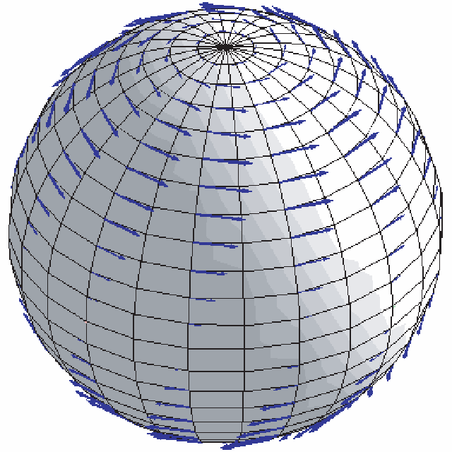
To gain further insight into the dynamics generated by (Symplectic approach to quantum constraints) we note that ${\mathcal{Q}}$ is the product of two Bloch spheres. Any motion on ${\mathcal{Q}}$ thus corresponds to a pair of coupled trajectories on these spheres. In terms of the usual spherical coordinates $(\{\theta_{i}\},\{\phi_{i}\})_{i=1,2}$ a point on ${\mathcal{Q}}$ can be written in the form $|\psi_{1}\rangle|\psi_{2}\rangle$, where

$\displaystyle|\psi_{i}\rangle=\cos\mbox{$\textstyle\frac{1}{2}$}\theta_{i}|\!\!\uparrow\rangle+\sin\mbox{$\textstyle\frac{1}{2}$}\theta_{i}\,\mbox{$\rm e$}^{{\rm i}\phi_{i}}|\!\!\downarrow\rangle.$

(52)

The idea of visualising the motions on the spheres is to express the phase-space coordinates $(\{q_{i}\},\{p_{i}\})$ in terms of the spherical coordinates $(\{\theta_{i}\},\{\phi_{i}\})$. For this, we must specify a Hamiltonian so that we can establish the relation between the energy eigenstates and the four chosen basis states $|\!\!\uparrow\uparrow\rangle,|\!\!\uparrow\downarrow\rangle,|\!\!\downarrow\uparrow\rangle,|\!\!\downarrow\downarrow\rangle$ on ${\mathcal{Q}}$. For example, suppose that the Hamiltonian takes the form

$\displaystyle{\hat{H}}=-J{\hat{\boldsymbol{\sigma}}}_{1}\otimes{\hat{\boldsymbol{\sigma}}}_{2}-B(\hat{\sigma}^{z}_{1}\otimes{\mathds{1}}_{2}+{\mathds{1}}_{1}\otimes\hat{\sigma}^{z}_{2}),$

(53)

which is a Heisenberg-type spin-spin interaction with strength $J$ and an external $z$-field with strength $B$. The eigenstates of this Hamiltonian are given by the spin-$0$ singlet state and the spin-$1$ triplet states. By comparing the coefficients of $|\psi_{1}\rangle|\psi_{2}\rangle$ with (26) one can express $(\{q_{i}\},\{p_{i}\})$ in terms of $(\{\theta_{i}\},\{\phi_{i}\})$. We invert the resulting relations to obtain

$\displaystyle\begin{array}[]{ccl}\theta_{1,2}&=&\sin^{-1}\sqrt{p_{2}+p_{3}-2\sqrt{p_{1}p_{4}}}\pm\cos^{-1}\sqrt{p_{1}+p_{4}-\sqrt{p_{1}p_{4}}}\\ \phi_{1,2}&=&-\frac{1}{2}\left(q_{1}\pm\cos^{-1}\left(\mbox{$\textstyle\frac{1}{2}$}(p_{3}-p_{2})/\sqrt{p_{1}p_{4}}\right)\right),\end{array}$

where $(\theta_{1},\phi_{1})$ corresponds to the ‘$+$’ sign and $(\theta_{2},\phi_{2})$ corresponds to the ‘$-$’ sign in the right side of (Symplectic approach to quantum constraints). From (Symplectic approach to quantum constraints) and (Symplectic approach to quantum constraints) we deduce the equations of motion in terms of the spherical variables, with the results:

$\displaystyle\begin{array}[]{l}\dot{\theta}_{1}=\dot{\theta}_{2}=0\\ \dot{\phi}_{1}=\dot{\phi}_{2}=-\mbox{$\textstyle\frac{1}{2}$}(\omega_{1}-\omega_{2}-\omega_{3})(\sin^{2}\mbox{$\textstyle\frac{1}{2}$}\theta_{1}+\sin^{2}\mbox{$\textstyle\frac{1}{2}$}\theta_{2})-\mbox{$\textstyle\frac{1}{2}$}(\omega_{2}+\omega_{3}).\end{array}$

We thus find that for a given initial state the dynamical trajectories are given by a pair of latitudinal circles on the respective Bloch spheres. An example of a field plot for one of the Bloch spheres is shown in Figure 1.

Example 2. We consider a system of three spin-$\frac{1}{2}$ particles, and impose the restriction that the unitary evolution is constrained to lie on a product space $\mathcal{R}=\mathcal{P}^{1}\times\mathcal{P}^{1}\times\mathcal{P}^{1}$ that contains the energy eigenstates. In this case, a necessary and sufficient condition for the state $|\psi\rangle$ to lie on $\mathcal{R}$ is that the components of the state vector simultaneously satisfy two quadratic equations [18]. Expressed in terms of the homogeneous coordinates $\{\psi_{i}\}_{i=1,2,\ldots,8}$ of $|\psi\rangle$ we find that the relevant constraints are given by four complex equations: $\psi_{1}\psi_{7}=\psi_{3}\psi_{4}$, $\psi_{2}\psi_{8}=\psi_{5}\psi_{6}$, $\psi_{1}\psi_{8}=\psi_{2}\psi_{7}$, and $\psi_{3}\psi_{6}=\psi_{4}\psi_{5}$. Taking the real and the imaginary parts of these equations and expressing the results in terms of $(\{q_{i}\},\{p_{i}\})$ we obtain the following eight constraints:

$\displaystyle\begin{array}[]{l}\Phi^{1}=q_{2}-q_{5}-q_{6}\\ \Phi^{2}=q_{1}+q_{7}-q_{3}-q_{4}\\ \Phi^{3}=q_{1}-q_{2}-q_{7}\\ \Phi^{4}=q_{3}+q_{6}-q_{4}-q_{5}\\ \Phi^{5}=p_{2}p_{8}-p_{5}p_{6}\\ \Phi^{6}=p_{1}p_{7}-p_{3}p_{4}\\ \Phi^{7}=p_{1}p_{8}-p_{2}p_{7}\\ \Phi^{8}=p_{3}p_{6}-p_{4}p_{5},\end{array}$

where we have written $p_{8}=1-\sum_{i=1}^{7}p_{i}$. Remarkably, the constraint equations for the variables $\{q_{i}\}$ and $\{p_{i}\}$ decouple. We can also read off from (Symplectic approach to quantum constraints) the condition for the unitary motion to lie on $\mathcal{R}$:

$\displaystyle\begin{array}[]{l}\omega_{1}=\omega_{2}+\omega_{7}\\ \omega_{2}=\omega_{5}+\omega_{6}\\ \omega_{1}+\omega_{7}=\omega_{3}+\omega_{4}\\ \omega_{3}+\omega_{6}=\omega_{4}+\omega_{5}.\end{array}$

It follows that the eigenvalues of the trace-free part of the Hamiltonian must take the form $\{e_{1},e_{2},e_{3},e_{4},-e_{4},-e_{3},-e_{2},-e_{1}\}$.

If ${\hat{H}}$ does not have this property, then the constraints (Symplectic approach to quantum constraints) become nontrivial. Nevertheless, owing to the fact that they decouple it is straightforward to verify that the equations of motion are given by $\dot{q}_{i}=f_{i}(\{p_{i}\})$ and $\dot{p}_{i}=0$ for $i=1,\ldots,7$, where $f_{i}(\{p_{i}\})$ are elementary functions of the variables $\{p_{i}\}$. It follows that the dynamical evolution is quasi-unitary in that the amplitudes $\{p_{i}\}$ remain constant and the relative phases $\{p_{i}\}$ evolve linearly in time.

Example 3. Let us turn to a different example. We consider again a pair of spin-$\frac{1}{2}$ particles and impose the condition that an initially disentangled quantum state remains disentangled under the dynamics. This constraint can be expressed algebraically by requiring that the motion is confined to the special quadric $\mathcal{Q^{\prime}}$ that corresponds to disentangled spin states. A generic state is still given by (26) but it is now no longer the case that all the energy eigenstates $|E_{i}\rangle$ lie on $\mathcal{Q}^{\prime}$. In other words, the constraint surface is no longer given by $\psi_{1}\psi_{4}=\psi_{2}\psi_{3}$ in the energy basis.

For the specification of the constraint equation associated with disentangled states, we must specify the Hamiltonian. We consider the Heisenberg-type spin-spin interaction system given by (53). The corresponding energy eigenstates include the total spin-$0$ singlet state and the total spin-$1$ triplet states. We then change basis by substituting the energy eigenstates in (26) with the singlet and triplet spin states such that we can express our general state in terms of the four disentangled basis states $|\!\!\uparrow\uparrow\rangle,|\!\!\uparrow\downarrow\rangle,|\!\!\downarrow\uparrow\rangle,|\!\!\downarrow\downarrow\rangle$ of $\mathcal{Q}^{\prime}$. We find

	$\displaystyle|\psi\rangle$	$\displaystyle=$	$\displaystyle{\surd p_{4}}|\!\!\uparrow\uparrow\rangle+\frac{1}{{\surd 2}}({\surd p_{2}}\mbox{$\rm e$}^{-{\rm i}q_{2}}-{\surd p_{3}}\mbox{$\rm e$}^{-{\rm i}q_{3}})|\!\!\uparrow\downarrow\rangle$		(74)
			$\displaystyle+\frac{1}{{\surd 2}}({\surd p_{2}}\mbox{$\rm e$}^{-{\rm i}q_{2}}+{\surd p_{3}}\mbox{$\rm e$}^{-{\rm i}q_{3}})|\!\!\downarrow\uparrow\rangle+{\surd p_{1}}\mbox{$\rm e$}^{-{\rm i}q_{1}}|\!\!\downarrow\downarrow\rangle.$

Since all the basis states used in (74) lie on $\mathcal{Q}^{\prime}$, now we are able to use the condition $\psi_{1}\psi_{4}=\psi_{2}\psi_{3}$ to constrain the motion on $\mathcal{Q}^{\prime}$:

$\displaystyle\sqrt{p_{1}p_{4}}\mbox{$\rm e$}^{-{\rm i}q_{1}}=\mbox{$\textstyle\frac{1}{2}$}(p_{2}\mbox{$\rm e$}^{-2{\rm i}q_{2}}-p_{3}\mbox{$\rm e$}^{-2{\rm i}q_{3}}).$

(75)

Taking the real and imaginary part of (75) we find that the two constraints required for the motion to remain on $Q^{\prime}$ are

$\displaystyle\begin{array}[]{l}\Phi_{1}=2\sqrt{p_{1}p_{4}}-p_{2}\cos(2q_{2}-q_{1})+p_{3}\cos(2q_{3}-q_{1})=0\\ \Phi_{2}=p_{2}\sin(2q_{2}-q_{1})-p_{3}\sin(2q_{3}-q_{1})=0.\end{array}$

Unlike the previous examples, these constraints are not separable, hence we can no longer expect to find the quasi-unitary motion seen in the previous cases. Substituting the constraints (Symplectic approach to quantum constraints) into (15) and following the procedures, we find that the resulting equations of motion are given by

$\displaystyle\begin{array}[]{l}\dot{p}_{1}=2p_{2}p_{3}(\omega_{1}-\omega_{3})\sin(2(q_{2}-q_{3}))\\ \dot{p}_{2}=-2p_{2}p_{3}(\omega_{1}-2\omega_{3})\sin(2(q_{2}-q_{3}))\\ \dot{p}_{3}=2p_{2}p_{3}(\omega_{1}-2\omega_{2})\sin(2(q_{2}-q_{3}))\\ \dot{q}_{1}=2p_{3}(1-2p_{1}-p_{2}-p_{3})(\omega_{2}-\omega_{3})\cos(2q_{3}-q_{1})/\sqrt{p_{1}p_{4}}\\ \qquad+(\omega_{1}-2\omega_{2})(2p_{1}+p_{2}+p_{3})+2\omega_{2}\\ \dot{q}_{2}=2p_{1}p_{3}(\omega_{3}-\omega_{2})\cos(2q_{3}-q_{1})/\sqrt{p_{1}p_{4}}+(\omega_{1}-2\omega_{2})(2p_{1}+p_{2})-p_{3}(\omega_{1}-2\omega_{3})+2\omega_{2}\\ \dot{q}_{3}=2p_{1}p_{3}(\omega_{3}-\omega_{2})\cos(2q_{3}-q_{1})/\sqrt{p_{1}p_{4}}\\ \qquad+(\omega_{1}-2\omega_{2})(2p_{1}-p_{2}\cos(2(q_{2}-q_{3})))+p_{3}(\omega_{1}-2\omega_{3})+2\omega_{3}.\\ \end{array}$

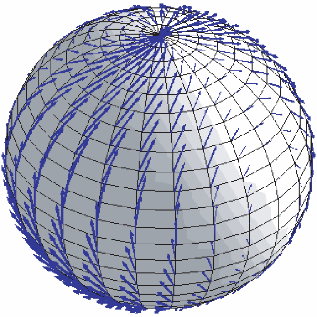
It is no longer the case that $\dot{p}_{i}=0$. Therefore, we have six coupled nonlinear differential equations describing the motion. We can visualise the motion on the product of two Bloch spheres by converting (Symplectic approach to quantum constraints) into spherical coordinates:

$\displaystyle\begin{array}[]{l}\dot{\theta}_{1}=\sin(\phi_{1}-\phi_{2})\sin\theta_{2}[(\omega_{1}-\omega_{2})\cos\theta_{1}+\omega_{2}-\omega_{3}]\\ \dot{\theta}_{2}=\sin(\phi_{1}-\phi_{2})\sin\theta_{1}[(\omega_{2}-\omega_{1})\cos\theta_{2}-\omega_{2}+\omega_{3}]\\ \dot{\phi}_{1}=\frac{1}{2}[-\omega_{1}+(\omega_{2}-\frac{\omega_{1}}{2})\cos\theta_{2}+(\frac{3}{2}\omega_{1}-\omega_{2}-2\omega_{3})\cos\theta_{1}+[\cos(\phi_{1}-\phi_{2})/(\sin\theta_{1}\sin\theta_{2})]\\ \qquad\quad\times\left.\left(2(\omega_{3}-\omega_{2})\sin^{2}\theta_{1}\cos\theta_{2}+(\omega_{1}-\omega_{2})(\cos^{2}\theta_{1}-\cos^{2}\theta_{2})\right)\right]\\ \dot{\phi}_{2}=\frac{1}{2}[-\omega_{1}+(\omega_{2}-\frac{\omega_{1}}{2})\cos\theta_{1}+(\frac{3}{2}\omega_{1}-\omega_{2}-2\omega_{3})\cos\theta_{2}+[\cos(\phi_{1}-\phi_{2})/(\sin\theta_{1}\sin\theta_{2})]\\ \qquad\quad\times\left.\left(2(\omega_{3}-\omega_{2})\cos\theta_{1}\sin^{2}\theta_{2}-(\omega_{1}-\omega_{2})(\cos^{2}\theta_{1}-\cos^{2}\theta_{2})\right)\right].\end{array}$

An example of the resulting field plot arising from these equations is shown in Figure 2, indicating the nontrivial nature of the dynamics.

In summary, we see that constrained quantum motions of the Dirac type can be treated straightforwardly by means of the prescription described above. The resulting dynamical equations are in general quite intricate, and typically require numerical analysis.

The authors thank D. Holm and M. Parry for stimulating discussions. This work was carried out in part while DCB and LPH were visitors at the Perimeter Institute for Theoretical Physics, Waterloo, Ontario.

References

- [1] Strocchi, F. 1966 Complex coordinates and quantum mechanics. Rev. Mod. Phys. 38, 36–40.
- [2] Cantoni, V. 1977 The Riemannian structure on the states of quantum-like systems. Comm. Math. Phys. 56, 189–193.
- [3] Kibble, T. W. B. 1979 Geometrisation of quantum mechanics. Commun. Math. Phys. 65, 189–201.
- [4] Weinberg, S. 1989 Testing quantum mechanics. Ann. Phys. 194, 336–386.
- [5] Cirelli, R, Mania, A, Pizzocchero, L. 1990 Quantum mechanics as an infinite-dimensional Hamiltonian system with uncertainty structure. I, II. J. Math. Phys. 31, 2891–2903.
- [6] Gibbons, G. W. 1992 Typical states and density matrices. J. Geom. Phys. 8, 147–162.
- [7] Hughston, L. P. 1995 Geometric aspects of quantum mechanics. In Twistor Theory ed S Huggett (New York: Marcel Dekker, Inc.).
- [8] Ashtekar, A. & Schilling, T. A. 1995 Geometry of quantum mechanics. CAM-94 Physics Meeting, in AIP Conf. Proc. 342, 471–478, ed. Zapeda, A. (AIP Press, Woodbury, New York).
- [9] Brody, D. C. & Hughston, L. P. 2001 Geometric quantum mechanics. J. Geom. Phys. 38, 19–53.
- [10] Lüders G 1951 “Über die Zustandsänderung durch den Messprozess” Ann. Physik 8 322-328.
- [11] Dirac, P. A. M. 1950 Generalized Hamiltonian dynamics. Canadian J. Math. 2, 129–148.
- [12] Dirac, P. A. M. 1958, Generalised Hamiltonian dynamics. Proc. R. Soc. London A246, 326–332.
- [13] Burić, N. 2007 Hamiltonian quantum dynamics with separability constraints. Preprint (arXiv:0704.1359).
- [14] Corichi, A. 2008 On the geometry of quantum constrained systems. Preprint (arXiv:0801.1119).
- [15] Mielnik, B. 1974 Generalized quantum mechanics. Commun. Math. Phys. 37, 221–256.
- [16] Oh, P. & Kim, M. 1994 Action angle variables for complex projective space and semiclassical exacness. Mod. Phys. Lett. A9, 3339–3346.
- [17] Mielnik, B. 1980 Mobility of nonlinear systems. J. Math. Phys. 21, 44–54.
- [18] Brody, D. C., Gustavsson, A. C. T. & Hughston, L. P. 2007 Entanglement of 3-qubit geometry. J. Phys. Conf. Ser. 67, 012044-16.