Exclusive decay to double at next-to-leading order in
Abstract
Within the nonrelativistic QCD (NRQCD) factorization framework, we calculate the exclusive decay process to next-to-leading order in the strong coupling constant, while at leading order in the charm quark relative velocity. It is found that this new contribution to the amplitude is comparable in magnitude with the previously calculated relativistic correction piece, but differs by a phase about . Including this new contribution will increase the previous prediction to substantially, thus brightening the discovery potential of this clean hadronic decay channel of in the forthcoming LHC experiment.
The quest for the meson, the lowest-lying pseudoscalar bottomonium state, started shortly after the discovery of in 1977. A thorough understanding of its properties, such as its mass and decay pattern, will be great benefit to strengthening our knowledge towards heavy quarkonium physics [1].
Tremendous efforts have been invested in various high energy collision experiments during the past thirty years to seek this elusive particle, but convincing evidence about its existence has not emerged until very recently. After many futile searches, there finally comes out an exciting news from Babar collaboration last month [2], which reported the first unambiguous sighting of with a significance, through the hindered magnetic dipole transition process . It is interesting to note the rather precisely measured hyperfine - mass splitting, MeV, can play a decisive role in discriminating different quarkonium models [1].
Aside from its mass, almost nothing is known about the dynamical properties of the , e.g., its decay pattern. Owning to the weaker QCD coupling at bottom mass scale, together with the copious phase space opened up for innumerable decay channels, one in general expects that each exclusive decay mode may only be allotted a rather small branching ratio. Indeed, a rough estimate of some 2-body and 3-body hadronic decay channels of supports this expectation, and probably disintegrates primarily into final states of high multiplicities [3].
Some “golden” modes have been proposed for hunting , such as [4] and [5, 6]. Despite very clean signature thanks to the presence of , these decay modes unfortunately have rather suppressed branching ratios. Obviously, the collision experiments like factory are not well suited to pin down these decay modes due to the relatively low yield. By contrast, high energy hadron collision experiments in general possess a much larger production rate, which in turn allows for triggering these rare but very clean decay modes. For the decay , the original hope is that it should be discoverable in Tevatron Run 2 [4]. Subsequent investigation reveals the situation may not be so optimistic [7, 3] 11 1 Note there recently appeared an estimate for this process based on a final-state interaction model, in which first annihilates into , and the charm meson pair subsequently scatter into double [8]. The corresponding prediction critically hinges on the branching ratio of , which is poorly known at present. However, there is reasonable argument that suggests this ratio may be rather suppressed [3].. In particular, an explicit NRQCD calculation predicts , which implies that notwithstanding the pessimistic prospect of observing this decay channel in Tevatron Run 2, the chance may still be bright in the forthcoming LHC program [3].
The exclusive decay , apart from its phenomenological interest, is worthy of theoretical exploration in its own right. Since this hard exclusive process comprises entirely heavy quarkonium, it can serve as an ideal laboratory to test the applicability of NRQCD and perturbative QCD [9]. Note this process is quite similar to the double charmonium production processes at factory, e.g. , which have stirred quite a few attention since the first Belle measurements were released in 2002 [10] (for an incomplete list about NRQCD-based investigation, see [11, 12, 13, 14, 15, 16, 17, 18, 19, 20]). No doubt a systematic study of this hadronic decay process will offer complementary insight towards understanding the decay and production mechanisms of quarkonium.
A peculiar feature of the decay is that 22 2 This decay can also proceed through . Since this QED contribution is much less important than its QCD counterpart, it will be neglected in this work., at the lowest order in and charm quark relative velocity in , , the amplitude vanishes. Therefore, to obtain a non-vanishing result, one must proceed to the higher orders either in or . In Ref. [3], the leading relativistic correction to the tree-level process was explored. In this work, we make progress along the alternative route, i.e., we compute the correction but stay at the zeroth order in . Since , the latter contribution is expected to be as important as the former one, so it will be definitely desirable to work out this missing piece.
Before presenting our main result, it is instructive to recall some dynamical properties about this process. Let and stand for the helicities of two mesons in the rest frame. According to the helicity selection rule and angular momentum conservation, the decay configuration (, )=(0, 0) exhibits the slowest asymptotic decrease with , [21]. However, it is impossible for to decay into two longitudinally polarized because of conflict between parity and Lorentz invariance. The hadron helicity conservation, , can be violated either by the nonzero charm mass or by the transverse momentum of inside , . For every unit of deviation of this rule, there is a further suppression factor of or . For the only physically allowed helicity configurations (, )=(, ), the selection rule is violated by two units, so one expects no matter the cause of violation is due to nonzero or nonzero .
A noteworthy finding is that, at the lowest order in , the violation of the rule should be ascribable to the nonzero transverse momentum of in , instead of the nonzero [3]. The corresponding branching ratio exhibits the following asymptotic scaling
| (1) |
where the subscript emphasizes the corresponding contribution comes from the relativistic correction. The factor affiliated with the would-be “leading-power” scaling, stems from the squares of the wave functions at the origin of two , since . In the last equation has been assumed.

One may naturally wonder how the situation becomes when one goes to the next-to-leading order (NLO) in . Some typical NLO Feynman diagrams contributing to are shown in Fig. 1. Should it also be obligatory to retain finite relative momentum of in order to obtain a non-vanishing result? To answer this question, it is helpful to draw some clue from an analogous hadronic decay process, , which also violates the helicity selection rule. In this decay process, the lowest-order diagrams start already at one-loop, i.e., at , which in fact share the same topology as those represented by Fig. 1e). There it is found that keeping a nonzero but neglecting the relative momentum of is sufficient to give rise to a non-vanishing result [22]. This may be reckoned as a persuasive hint that a similar pattern may occur in our case. A more direct evidence comes from inspecting the cut structure of Fig. 1. It is easy to observe that all the diagrams in Fig. 1 [except Fig. 1e)] permit a specific cut that has a clear physical meaning, i.e., a cut through two intermediate gluon lines that divides the full process into and . Since both sub-processes are finite at the zeroth order in , so does the corresponding portion of the imaginary part of the amplitude which is obtained by stitching both on-shell sub-amplitudes together in accordance with the recipe of Cutkosky rule. Since a fraction of the imaginary part of the total amplitude is nonzero, there is no reason to expect the full imaginary part should vanish, thus we are reassured that at this order, the nonzero can adequately play the role of violating the helicity selection rule, and it suffices to set the relative velocity to zero in the calculation. As a result, we expect the NLO perturbative contribution scales as follows
| (2) |
where the subscript stresses the corresponding contribution comes from the perturbative correction. As will be confirmed by the explicit calculation, this power-law scaling indeed holds besides logarithmical scaling violation effect.
Having said this much, let us now proceed to the actual calculation. We first set up some notations. Let signify the momentum and polarization vector of each . Owning to parity and Lorentz invariance, the decay amplitude is constrained of the following structure:
| (3) |
Apparently, the only allowed helicity configurations indeed are . All the nontrivial dynamics is encoded in the reduced amplitude , and our task is then to unravel its explicit form.
In total 80 diagrams can be drawn for this process at . A full treatment of these diagrams, at first sight, may seem to be a daunting task. Luckily, the calculation turns out to be much simpler than one would imagine, thanks to some gratifying traits of this process. First, renormalization is not needed in this work. This originates from the fact that the amplitude at leading order in and vanishes. Since the contribution of the counterterm diagrams are proportional to the LO diagram, they simply vanish too. As a consequence, all the diagrams which contain primitive ultraviolet (UV) divergent subgraph must instead be free of the UV divergences, otherwise these unremoved divergences would signal the failure of the renormalization theory. A remarkable property of this process is that, these superficially UV-divergent diagrams are not only finite, in fact all of them vanish. Similarly, among the remaining manifestly UV-finite diagrams, a simplification further occurs, namely many diagrams with a symmetric topology also vanish, e.g., diagrams involving one 4-gluon vertex, diagrams involving two 3-gluon vertices, and diagrams containing a gluon ladder between the and lines. This can be mainly attributed to the specific Lorentz structure as indicated in (3), that is, in these diagrams, the Levi-Civita tensor that arises from the annihilation amplitude, is either contracted with some symmetric Lorentz indices, or there are no sufficient number of independent 4-vectors to contract with it.
There finally survive 40 diagrams with non-vanishing contribution, some of which are shown in Fig. 1a)-e). In fact, because of the interchanging symmetry between two , diagrams of a given topology usually give rise to an identical answer, and practically only much fewer diagrams need to be calculated. We employ the automated Feynman Diagram Calculation package (FDC) to fulfill the analytic evaluation of the required one-loop diagrams. FDC is a powerful program based on the symbolic language Reduce, which is designed to automate the perturbative quantum field theory calculation in computer. FDC was initially developed by one of us long ago [23], and the function of automatic one-loop calculation has recently been realized by two of us [24]. Recently, FDC has been successfully applied to several important quarkonium production processes to compute the NLO perturbative corrections [19, 20].
In passing, we would like to comment on some specific issues in the calculation. One technical complication is the occurrences of six-point one-loop integrals in Fig. 1a) and b). FDC has implemented some systematic recursive algorithm to reduce higher-point integrals down to lower-point ones. In this work, it turns out that all the encountered 6-point integrals can be reduced to the 4-point integrals and lower ones. In addition, Passarino-Veltman algorithm [25] has also been built into FDC to expedite the reduction of tensor integrals to the scalar ones.
It turns out that each individual diagram is infrared finite, at least in the Feynman gauge as we worked with. At a glance, one may feel that some care needs to be paid in handling Fig. 1b), since the Coulomb divergences may potentially arise there. Hearteningly, a close examination shows that this diagram is in fact free of any singular poles. The absence of Coulomb singularity can be most transparently understood in the NRQCD factorization ansatz [9]. What we can calculate within perturbation theory is the so-called hard (short-distance) coefficient. All the long-distance singularities encountered in computing the one-loop QCD diagrams, must be exactly reproduced in the respective one-loop NRQCD diagrams with a potential gluon attached between the outgoing - lines that forms a , so they ultimately cancel out in the intended hard coefficient via the matching procedure. However, the corresponding diagrams in the NRQCD sector trivially vanish in our case, again because the process vanishes at LO in and , therefore no any net long-distance divergence, such as Coulomb divergence, should be expected to appear in the diagrams in the QCD sector.
Finally it may be worthwhile to compare our process with . As stated earlier, the latter process is described by a small subset of Fig. 1, the class of diagrams exemplified by Fig. 1e), in which three “Abelian” gluons connect between quark line and the charm quark lines. Since has negative parity, charge conjugation invariance demands that three gluons must form a totally symmetric color-singlet state, therefore only the fully symmetric part of the color factor can contribute in this decay process [22]. On the contrary, due to the positive parity of , in our case the three gluons must instead be totally antisymmetric in color space, so the piece finally survive in the color factor. We have explicitly checked this is indeed the case.
After analytic manipulation of all the diagrams by FDC, together with some simplifying by hand, we can express the reduced amplitude as following:
| (4) |
where the relativistic normalization is used for the quarkonium states, and is the magnitude of momentum. The complex-valued function, which has encompassed the loop contribution, is deliberately chosen as dimensionless, therefore it can depend on and only through their dimensionless ratio . Furthermore, the function is normalized such that it varies with only logarithmically, which is slower than any power law scaling. After some quick algebra, one can verify that Eq. (4) is in conformity to up to logarithmical modification.
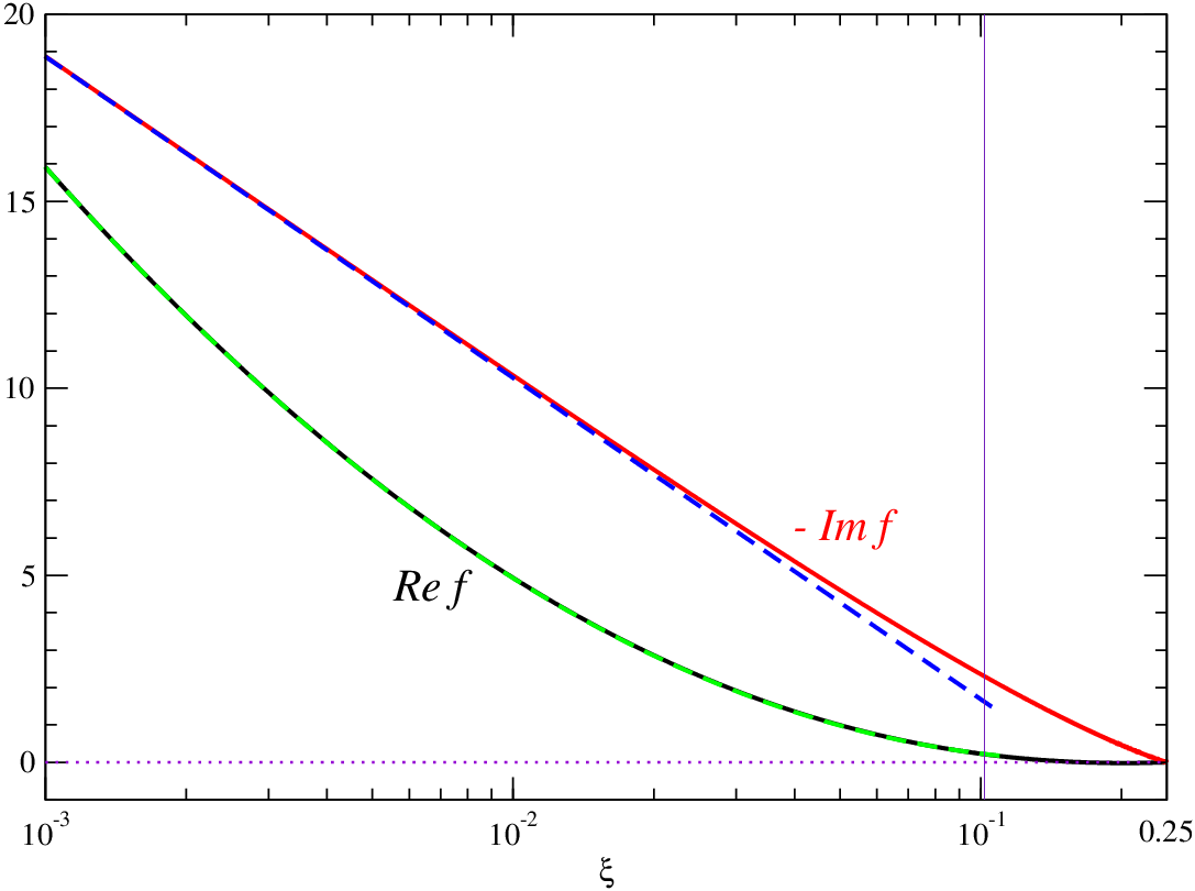
We display the shape of the function in Figure 2. The analytic expression for the real part of the function is too lengthy to be reproduced here. However, the analytical result for the imaginary part is quite compact,
| (5) | |||||
where .
It is instructive to deduce the asymptotic behavior of in the small limit. After some efforts, we obtain
| (6) | |||||
| (7) |
As can be clearly visualized in Fig. 2, as , the real and imaginary parts of the function exhibit and dependence, respectively. This seems to be a generic trait of exclusive bottomonium decays to double charmonium, which is also seen in the analogous function in the process [22]. It is interesting to note that, up to the physically relevant point , which is obtained by substituting GeV and GeV, the asymptotic expressions in (6) and (7) still constitute decent approximations to the true expressions, where the agreement for the real part is especially satisfactory, and the agreement for the imaginary part is at 70% level. This may suggest that, if one is willing to carry out this calculation by hand yet without loss of accuracy, the most efficient way is to first expand the integrand in prior to performing the loop integrals.
It is interesting to note that, provided that is not overly small, say, , then is always bigger than . In particular, at the phenomenologically relevant point , we find the corresponding , and the real part seems to be practically negligible.
Since the NLO perturbative amplitude is dominated by its imaginary part, one may like to speculate which type of cuts might constitute the most important contribution. It might sound attractive to inquire whether that specific cut as mentioned earlier, the one acting upon two intermediate gluon lines that partitions the full process into and , would dominate over all other possible cuts. If this were the case, we would be happy because this process then could be endowed with a “plausible” physical picture – that it proceeds first through annihilation into two gluons, and these two gluons subsequently rescatter into double . Let us examine this conjecture concretely. With the aid of the Cutkosky rule, it is straightforward to deduce this particular fraction of the imaginary part of the function, which we call :
| (8) |
Note the occurrence of the term, which can be traced to the cut contribution from Fig. 1a), renders this function scale with quark masses as , so that the true scaling is violated. This is unacceptable and clearly indicates approximating the full imaginary part by this specific fraction is unjustified. Numerically for , we obtain , which is far off the true value . A careful investigation reveals that each diagram in Fig. 1 [except Fig. 1e)] possesses a rich cut structure, for example, Fig. 1a), b), d) allow for 6, 5, and 4 different kind of cuts, respectively. Among all the possible cuts, those which pass through one gluon line and another nonadjacent quark line generally lead to more involved expressions in (5). For a given diagram, it seems not profitable to single out one specific cut to mimic its full imaginary part. For example, only after the remaining cuts are included, the imaginary part of Fig. 1a) then has a sensible answer, free of the dangerous singularity.
We are now very close to the intended formula. For completeness, we still need the expression of the reduced amplitude that arises from the tree-level relativistic correction [3]
| (9) |
Roughly speaking, is a quantity related to the second derivative of the wave function at the origin for , which governs the size of relativistic corrections. In fact, this factor admits a rigorous definition as a ratio of NRQCD matrix elements [9, 11]:
| (10) |
where denotes the polarization vector of at its rest frame, and represent Pauli spinor fields in NRQCD, is the spatial covariant derivative. The matrix elements appearing in the above ratio are understood to be the renormalized ones. It is worth stressing that the sign of needs not necessarily to be positive.
Plugging equations (4) and (9) in the formula
| (11) |
we then obtain the desired partial width. Note the cubic power of momentum reflects that two are in relative -wave state. This formula has already taken into account the sum over transverse polarizations of two as well as their indistinguishability. It may be more convenient to present an explicit expression for the branching ratio, where the wave function at the origin of drops out,
| (12) | |||||
In deriving this, we have approximated the total width of by its hadronic width:
| (13) |
where the factor encodes the magnitude of NLO perturbative correction to [26]
denotes the number of active light flavors. One usually takes , by treating charm quark also as a massless parton. For , we get .
Equation (12) constitutes the key formula of this work. From this equation one can readily confirm the asymptotic behaviors anticipated in (1) and (2).

Let us now explore the numerical outcome of (12). The input parameters are , , , and , respectively. We take GeV and GeV. Obviously, our predictions are quite sensitive to the value assigned for the strong coupling constant. To account for the affiliated ambiguity, we slide the renormalization scale from to , corresponding to varying between 0.18 and 0.26. The wave function at the origin of can be extracted from its electric width:
| (14) |
where the first-order perturbative correction has been included. Using the measured electric width 5.55 keV [27], we obtain .
Among various input parameters, the least known about is . Nevertheless, there is a useful relation, first derived by Gremm and Kapustin by employing the equation of motion of NRQCD [28], which expresses this quantity in terms of the charm quark pole mass and the mass. To our purpose this relation reads [11]
| (15) |
Owing to the intrinsic ambiguity associated with the charm quark pole mass, a wide spectrum of estimates for is scattered in literature. Ref. [11] takes GeV in the analysis of double charmonium production at factory, which leads to from (15). Note this value is compatible with , which is obtained from a recent Cornell potential-model based analysis [29, 30]. A positive is helpful to alleviate the discrepancy between the LO NRQCD prediction and the measured production rate at Belle. Notwithstanding the phenomenological inclination, however, one may be alert that a rather different value might not be excluded on theoretical ground. For example, if GeV is assumed, which stems from a recent QCD moment sum rule analysis [31], one would instead obtain , whose sign has even changed. Because of the impossibility to nail down to an accuracy better than , it seems safe to take a conservative attitude, by assigning a rather large uncertainty to . In this work, we will assume , including the possibility that it may even vanish.
In Figure 3 we illustrate how the branching ratio of varies with and . In the left panel of Fig. 3, one can clearly see that inclusion of the QCD perturbative correction will significantly enhance the previous prediction that only implements relativistic correction, especially when is small. The approximately parabolic dependence of on , reflects the fact that the NLO perturbative amplitude, , is dominated by its imaginary part, therefore it is nearly orthogonal to the relativistic correction amplitude , so their contributions can be added almost incoherently. To see the interference pattern lucidly, we make a numerical presentation to the terms inside the absolute value sign in (12),
It is interesting to note, besides the approximate phase difference, the (imaginary part of) NLO perturbative contribution is comparable in magnitude with the relativistic correction piece. The residual interference between the real part of the perturbative correction amplitude and the relativistic correction piece has modest effect, which can be either constructive or destructive depending on the sign of . In the right panel of Fig. 3, one can further observe that, despite the acute sensitivity to the choice of the renormalization scale, the complete result is considerably larger than each individual contribution in the considered range of .
As can be inferred from Figure 3, our final estimate of the branching ratio is
| (16) |
Not surprisingly, the uncertainty is rather large. It is enlightening to compare our result with the previous prediction that includes only the relativistic correction contribution [3]:
| (17) |
Though the strategies of estimating the error differ in both work, it is nevertheless unambiguous to see the substantial effects of the NLO perturbative correction. It is worth mentioning that the lowest bound of our prediction is already as large as , which can be entirely attributed to the NLO perturbative contribution. In contrast, the prediction including only the relativistic correction simply vanishes as approaches zero.
Finally we present an updated estimate about the discovery potential of this decay mode in the LHC experiments. In the hadron collision experiment can be cleanly reconstructed via its muonic decay mode. Multiplying (16) by the branching ratios of 6% for each of the decay , we obtain . Assuming the production cross section at LHC to be about 15 [3], one then finds the cross section for the 4 events to be about 1-10 fb. For a 300 data, which is expected to be gleaned in one year run at LHC design luminosity, the number of produced events may reach 300-3000. The product of acceptance and efficiency for detecting decay to is estimated to be [4], which is perhaps a conservative estimate for LHC. Multiplying the number of the produced events by , we expect between 3 and 30 observed events per year. From this rough estimate, we are tempted to conclude that, the prospect of observing at LHC through the 4 mode looks promising. However, we should be fully aware that it will be a highly challenging task for experimentalists to single out the relatively few signal events from the presumedly abundant continuum background.
To summarize, in this work we have studied the exclusive decay process to NLO in while at LO in . We found that this new contribution to the amplitude is comparable in magnitude with the previously calculated tree-level relativistic correction piece, but differs by a phase about . Including this new piece of contribution will substantially enhance the previous estimate of , thus the observation prospect of this clean hadronic decay mode in the forthcoming LHC experiment becomes brighter.
Acknowledgements.
This work is supported in part by National Natural Science Foundation of China under Grants No. 10605031, 10475083, and by the Chinese Academy of Sciences under Project No. KJCX3-SYW-N2.References
- [1] N. Brambilla et al, CERN-2005-005 [arXiv:hep-ph/0412158], and references therein.
- [2] B. Aubert et al. [BABAR Collaboration], Phys. Rev. Lett. 101, 071801 (2008) [arXiv:0807.1086 [hep-ex]].
- [3] Y. Jia, Phys. Rev. D 78, 054003 (2008) [arXiv:hep-ph/0611130].
- [4] E. Braaten, S. Fleming and A. K. Leibovich, Phys. Rev. D 63, 094006 (2001) [arXiv:hep-ph/0008091].
- [5] G. Hao, Y. Jia, C. F. Qiao and P. Sun, JHEP 0702, 057 (2007) [arXiv:hep-ph/0612173].
- [6] Y. J. Gao, Y. J. Zhang and K. T. Chao, arXiv:hep-ph/0701009.
- [7] F. Maltoni and A. D. Polosa, Phys. Rev. D 70, 054014 (2004) [arXiv:hep-ph/0405082].
- [8] P. Santorelli, Phys. Rev. D 77, 074012 (2008) [arXiv:hep-ph/0703232].
- [9] G. T. Bodwin, E. Braaten and G. P. Lepage, Phys. Rev. D 51, 1125 (1995) [Erratum-ibid. D 55, 5853 (1997)] [arXiv:hep-ph/9407339].
- [10] K. Abe et al. [Belle Collaboration], Phys. Rev. Lett. 89, 142001 (2002) [arXiv:hep-ex/0205104].
- [11] E. Braaten and J. Lee, Phys. Rev. D 67, 054007 (2003) [Erratum-ibid. D 72, 099901 (2005)] [arXiv:hep-ph/0211085].
- [12] K. Y. Liu, Z. G. He and K. T. Chao, Phys. Lett. B 557, 45 (2003) [arXiv:hep-ph/0211181].
- [13] G. T. Bodwin, J. Lee and E. Braaten, Phys. Rev. Lett. 90, 162001 (2003) [arXiv:hep-ph/0212181].
- [14] G. T. Bodwin, J. Lee and E. Braaten, Phys. Rev. D 67, 054023 (2003) [Erratum-ibid. D 72, 099904 (2005)] [arXiv:hep-ph/0212352].
- [15] K. Hagiwara, E. Kou and C. F. Qiao, Phys. Lett. B 570, 39 (2003) [arXiv:hep-ph/0305102].
- [16] Y. J. Zhang, Y. j. Gao and K. T. Chao, Phys. Rev. Lett. 96, 092001 (2006) [arXiv:hep-ph/0506076].
- [17] Z. G. He, Y. Fan and K. T. Chao, Phys. Rev. D 75, 074011 (2007) [arXiv:hep-ph/0702239].
- [18] G. T. Bodwin, J. Lee and C. Yu, Phys. Rev. D 77, 094018 (2008) [arXiv:0710.0995 [hep-ph]].
- [19] B. Gong and J. X. Wang, Phys. Rev. D 77, 054028 (2008) [arXiv:0712.4220 [hep-ph]].
- [20] B. Gong and J. X. Wang, Phys. Rev. Lett. 100, 181803 (2008) [arXiv:0801.0648 [hep-ph]].
- [21]
S. J. Brodsky and G. P. Lepage,
Phys. Rev. D 24, 2848 (1981);
V. L. Chernyak and A. R. Zhitnitsky, Phys. Rept. 112, 173 (1984). - [22] Y. Jia, Phys. Rev. D 76, 074007 (2007) [arXiv:0706.3685 [hep-ph]].
- [23]
J. X. Wang and Y. Shimizu,
Prepared for 3rd International Workshop on Software
Engineering, Artificial Intelligence and Expert systems for
High-energy and Nuclear Physics, Oberammergau, Germany, 4-8 Oct
1993;
J. X. Wang, Nucl. Instrum. Meth. A 534, 241 (2004) [arXiv:hep-ph/0407058]. - [24]
B. Gong and J. X. Wang, in preparation;
B. Gong, PhD thesis, Development of automatic one-loop correction calculation in FDC and its applications, (IHEP, Beijing, 2008). - [25] G. Passarino and M. J. G. Veltman, Nucl. Phys. B 160, 151 (1979).
- [26] A. Petrelli, M. Cacciari, M. Greco, F. Maltoni and M. L. Mangano, Nucl. Phys. B 514, 245 (1998) [arXiv:hep-ph/9707223].
- [27] W. M. Yao et al. [Particle Data Group], J. Phys. G 33, 1 (2006).
- [28] M. Gremm and A. Kapustin, Phys. Lett. B 407, 323 (1997) [arXiv:hep-ph/9701353].
- [29] G. T. Bodwin, D. Kang and J. Lee, Phys. Rev. D 74, 014014 (2006) [arXiv:hep-ph/0603186].
- [30] G. T. Bodwin, H. S. Chung, D. Kang, J. Lee and C. Yu, Phys. Rev. D 77, 094017 (2008) [arXiv:0710.0994 [hep-ph]].
- [31] M. Eidemuller, Phys. Rev. D 67, 113002 (2003) [arXiv:hep-ph/0207237].