跳到论文正文
W Papers独立论文阅读器 arXiv:0808.0923 论文正文 计算阅读时间 · 0%
引用这篇论文根据当前论文元数据生成,正式投稿前建议核对。


License: arXiv.org perpetual non-exclusive license
arXiv:0808.0923v2 [hep-th] 04 Jun 2009

Center for the Fundamental Laws of Nature
Jefferson Physical Laboratory, Harvard University,
Cambridge, MA 02138 USA

agiombi@physics.harvard.edu, bxiyin@fas.harvard.edu

In this paper we show that Liouville gravity on the strip with Zamolodchikov-Zamolodchikov (ZZ) boundary conditions has a semi-classical interpretation in terms of fragmented A​d​S2AdS_{2} spacetime geometries. Further, we study the three-point functions of the ZZ boundary primaries, and show that they are dominated by multi-A​d​S2AdS_{2} instantons in the classical limit.

1 Introduction

Two-dimensional gravity has been extensively explored in the past 30 years, both as the worldsheet description of string theories and as a toy model for higher dimensional quantum gravity (for a review see [1] and references therein). Quantum gravity in A​d​S2AdS_{2}, which is expected to be related to extremal black holes, remains mysterious [2, 3, 4, 5, 6, 7]. In this paper, we shall take the viewpoint that “pure” quantum gravity in A​d​S2AdS_{2} is described by Liouville gravity, with Zamolodchikov-Zamolodchikov (ZZ) boundary conditions [8].11 1 For reviews of Liouville theory see for example [10] [11]. The states of quantum gravity in global A​d​S2AdS_{2} will be the boundary primaries of ZZ. This proposal will be validated by finding the semi-classical interpretation of these states and their correlation functions. We will see that in the semi-classical limit, the ZZ boundary primaries describe “fragmented” A​d​S2AdS_{2}’s, i.e. several global A​d​S2AdS_{2}’s “attached” along their boundaries. The correlation functions of the ZZ boundary primaries will be dominated by the contribution from classical instantons, which are several Poincaré discs suitably “glued” together along parts of their boundaries.

We analyze the quantum corrections to the two-fragmented A​d​S2AdS_{2} using the exact bulk-boundary three point functions on the disc. The radius of the A​d​S2AdS_{2} solution is large in the semi-classical (weak coupling) limit of Liouville gravity. In this limit, the Liouville theory has either large positive central charge cLc_{L} (with real background charge QQ), or large negative cLc_{L} (with imaginary QQ). In the cL>0c_{L}>0 case, we find that quantum corrections erase one of the two A​d​S2AdS_{2}’s. In the cL<0c_{L}<0 case, the two-fragmented A​d​S2AdS_{2} survive in the quantum theory.

From the point of view of A​d​S2/C​F​T1AdS_{2}/CFT_{1} correspondence, our results suggest that the “C​F​T1CFT_{1}” dual to pure Liouville gravity in A​d​S2AdS_{2} comprises a single copy of Virasoro alegbra and a finite set of primary states – those of Liouville theory on a strip with ZZ boundary conditions. The correlation functions of these primaries can in principle be computed exactly using bootstrap methods, which then completely characterizes the theory.

The paper is organized as follows. In section 2 we first review the ZZ boundary conditions and boundary primaries. We will then probe the “geometry” of the semi-classical limit of the ZZ boundary primary using a bulk primary operator, and show that the boundary primaries can be identified as fragmented A​d​S2AdS_{2}’s. In section 3 we study the three-point functions of the boundary primaries. Once again using the bulk primary probe, we will find that in the semi-classical limit the bulk-boundary four-point function is dominated by an instanton solution interpolating fragmented A​d​S2AdS_{2}’s.

2 ZZ boundary primaries as fragmented A​d​S2AdS_{2}

2.1 ZZ boundary conditions and boundary primaries in Liouville theory

We work in the convention of [8], and write the Liouville Lagrangian density (in a flat background metric) as

ℒ=14​π​(∂aϕ)2+μ​e2​b​ϕ.{\cal L}=\frac{1}{4\pi}(\partial_{a}\phi)^{2}+\mu e^{2b\phi}. (2.1)

The background charge is Q=b+1/bQ=b+1/b, and the central charge of the Liouville CFT is given by c=1+6​Q2c=1+6Q^{2}. Depending on whether bb is real or purely imaginary, the central charge cc is greater or less than 1. If bb is imaginary, we may retain a real Lagrangian density by Wick rotating ϕ→i​ϕ~\phi\to i\tilde{\phi}, and ϕ~\tilde{\phi} will have a wrong sign kinetic term. The Liouville field ϕ\phi can be thought of as the conformal mode of gravity in two dimensions, with metric

d​s2=e2​b​ϕ​δa​b​d​σa​d​σb.ds^{2}=e^{2b\phi}\delta_{ab}d\sigma^{a}d\sigma^{b}. (2.2)

The Liouville action is generated when a two-dimensional “matter” conformal field theory of nonzero central charge −c-c is coupled to gravity [12]. For the purpose of this paper, we can ignore the matter CFT, although we shall keep in mind that the full theory of quantum gravity should have total central charge zero.

The ZZ boundary condition is such that the expectation value of e2​b​ϕe^{2b\phi} goes to +∞+\infty at the boundary. Such consistent quantum boundary conditions are labeled by a pair of positive integers (m,n)(m,n). There is a symmetry which exchanges mm with nn while sending b→1/bb\to 1/b. Global A​d​S2AdS_{2} can be described as a classical solution of Liouville theory on a strip σ∈(0,π)\sigma\in(0,\pi), τ∈𝐑\tau\in{\bf R}, with e2​b​ϕ→+∞e^{2b\phi}\to+\infty on the two boundaries. In the quantum theory, we can choose independently (m,n)(m,n) boundary condition on the left side of the strip, and (m′,n′)(m^{\prime},n^{\prime}) on the right side of the strip. The Hilbert space of states on the strip will be denoted by ℋ(m,n,m′,n′){\cal H}_{(m,n;m^{\prime},n^{\prime})}. It consists of boundary primary states ψk,l\psi_{k,l} and their Virasoro descendants. The boundary primary ψk,l\psi_{k,l} is characterized by its conformal dimension

Δk,l=Q24−(k​b+l/b)24,\Delta_{k,l}=\frac{Q^{2}}{4}-\frac{(kb+l/b)^{2}}{4}, (2.3)

and is subject to the selection rule

k=|m−m′|+1,|m−m′|+3,⋯,m+m′−1;\displaystyle k=|m-m^{\prime}|+1,~|m-m^{\prime}|+3,~\cdots~,m+m^{\prime}-1; (2.4)
l=|n−n′|+1,|n−n′|+3,⋯,n+n′−1.\displaystyle l=|n-n^{\prime}|+1,~|n-n^{\prime}|+3,~\cdots~,n+n^{\prime}-1.

The bulk one-point function ⟨Vα​(z,z¯)⟩\langle V_{\alpha}(z,\bar{z})\rangle on the disc with boundary condition (m,n)(m,n), as well as the bulk-boundary two-point function (for special boundary operators), have been solved in [8]. We will need more: the bulk-boundary three-point function, boundary three-point function, and the bulk-to-boundary four-point function. These will be solved in the next few subsections by conformal bootstrap method.

2.2 Fragmented A​d​S2AdS_{2} as classical solutions

It is well known that the Liouville equation of motion on the strip (for simplicity we set henceforth μ=1\mu=1 in the action (2.1))

(∂σ2−∂t2)ϕ=4πbe2​b​ϕ(\partial^{2}_{\sigma}-\partial^{2}_{t})\phi=4\pi be^{2b\phi} (2.5)

admits the basic static solution

ϕ=−12​b​ln⁡(4​π​b2​sin2⁡σ).\phi=-\frac{1}{2b}\ln(4\pi b^{2}\sin^{2}\sigma)\,. (2.6)

Of course, the corresponding physical metric d​s2=e2​b​ϕ​(−d​t2+d​σ2)ds^{2}=e^{2b\phi}(-dt^{2}+d\sigma^{2}) is nothing but the A​d​S2AdS_{2} space-time. This is the S​L​(2,ℝ)SL(2,\mathbb{R}) invariant vacuum of Liouville theory first pointed out in [13],[14] (see also [2]).

It is easy to see that the A​d​S2AdS_{2} solution is part of a more general family of static solutions

ϕ=−12​b​ln⁡(4​π​b2​sin2⁡(l​σ)l2)\phi=-\frac{1}{2b}\ln\left(4\pi b^{2}\frac{\sin^{2}(l\sigma)}{l^{2}}\right) (2.7)

parameterized by an integer l≥1l\geq 1. These solutions behave like A​d​S2AdS_{2} at the σ=0,π\sigma=0,\pi boundaries, but the metric also blows up in the “interior” at σ=plπ,p=1,⋯,l−1\sigma=\frac{p}{l}\pi\,,p=1,\cdots,l-1. In other words, the corresponding space-time looks like ll disconnected copies of the A​d​S2AdS_{2} solution. An example with l=2l=2 is plotted in Fig. 1. We will refer to these solutions as “fragmented A​d​S2AdS_{2} spaces”.

A first hint to the relation between fragmented A​d​S2AdS_{2}’s and ZZ boundary primaries comes from looking at the classical Liouville stress tensor evaluated on the solutions (2.7). The T00T_{00} component of the stress tensor for a static solution reads

T00=14​π​(∂σϕ)2+e2​b​ϕ−12​π​b​∂σ2ϕ,T_{00}=\frac{1}{4\pi}(\partial_{\sigma}\phi)^{2}+e^{2b\phi}-\frac{1}{2\pi b}\partial^{2}_{\sigma}\phi\,, (2.8)

where the last term comes from the “linear dilaton” coupling to the 2d scalar curvature. Evaluated on (2.7), this just gives the constant T00=−l24​π​b2T_{00}=-\frac{l^{2}}{4\pi b^{2}}. Then one would obtain an energy relative to the A​d​S2AdS_{2} vacuum

E=−l2−14​b2.E=-\frac{l^{2}-1}{4b^{2}}\,. (2.9)

Note that this result precisely matches the classical limit b→0b\rightarrow 0 of the conformal dimension Δk,l\Delta_{k,l} of the ZZ boundary primaries, eq. (2.3) (kk drops out of the classical limit, as long as it is much smaller than 1b2\frac{1}{b^{2}}).

2.3 The classical limit of bulk-boundary three point functions

A given ZZ boundary primary |ψ⟩|\psi\rangle should correspond to a deformation of the Liouville profile (i.e. the space-time metric) in the bulk. Specifically, we would like to argue that the relevant bulk metrics in the classical limit b→0b\rightarrow 0 correspond to the “fragmented” A​d​S2AdS_{2} spaces (2.7). To test this idea, we shall study the expectation value ⟨ϕ⟩\langle\phi\rangle of the Liouville field on the strip, in a boundary primary state |ψ⟩|\psi\rangle. This can be done by using as a “probe” the bulk primary operator Vα=e2​α​ϕV_{\alpha}=e^{2\alpha\phi}. More precisely, we need to compute the disc bulk-boundary three point function

⟨ψ⁡(y1)​ψ​(y2)​Vα​(z,z¯)⟩=|z−z¯|−2​Δα​(y1−y2)−2​h​ℱ​(η)\langle\psi(y_{1})\psi(y_{2})V_{\alpha}(z,\bar{z})\rangle=|z-\bar{z}|^{-2\Delta_{\alpha}}(y_{1}-y_{2})^{-2h}{\cal F}(\eta) (2.10)

where Δα=α⁡(Q−α)\Delta_{\alpha}=\alpha(Q-\alpha) is the dimension of VαV_{\alpha}, hh is the dimension of ψ\psi, and η\eta is the S​L​(2,ℝ)SL(2,{\mathbb{R}}) invariant cross ratio

η=(z−z¯)​(y1−y2)(z−y2)​(y1−z¯)=1−e2​i​σ,\eta=\frac{(z-\bar{z})(y_{1}-y_{2})}{(z-y_{2})(y_{1}-\bar{z})}=1-e^{2i\sigma}\,, (2.11)

where σ\sigma is the spatial coordinate on the strip (to obtain this relation, one can use S​L​(2,ℝ)SL(2,\mathbb{R}) to set y1=0,y2=∞y_{1}=0\,,y_{2}=\infty). The three point function (2.10) is interpreted as the expectation value ⟨ψ|Vα​(σ)|ψ⟩\langle\psi|V_{\alpha}(\sigma)|\psi\!\rangle in the ZZ boundary primary |ψ⟩|\psi\rangle. When ψ\psi is the identity operator, this is just the bulk one-point function computed by ZZ [8]

⟨Vα​(z,z¯)⟩=U⁡(α)|z−z¯|2​Δα.\langle V_{\alpha}(z,\bar{z})\rangle=\frac{U(\alpha)}{|z-\bar{z}|^{2\Delta_{\alpha}}}\,. (2.12)

Transforming back to strip coordinates z=ei​σ+τz=e^{i\sigma+\tau}, one can see that in fact this is just the A​d​S2AdS_{2} metric (2.6).

The correlation function (2.10) depends of course on the explicit choice of (m,n)(m,n) boundary conditions. For now we keep the analysis general and do not specify the type of boundary conditions. Let us consider the simplest nontrivial example, ψ=ψ1,2\psi=\psi_{1,2}. According to (2.3)(\ref{conf-dim}), it has conformal dimension

h1,2=−12−34​b2.h_{1,2}=-\frac{1}{2}-\frac{3}{4b^{2}}. (2.13)

All ZZ boundary primaries are degenerate, i.e. their conformal families contains null states. In particular, the conformal family of ψ1,2\psi_{1,2} has a null state at level two, namely (L−12+b−2​L−2)​|ψ1,2⟩=0(L_{-1}^{2}+b^{-2}L_{-2})|\psi_{1,2}\rangle=0. It follows that the bulk-boundary three point function satisfies the differential equation

{∂y12+b−2[h1,2(y2−y1)2+Δα(z−y1)2+Δα(z¯−y1)2\displaystyle\left\{{\partial_{y_{1}}^{2}}+b^{-2}\left[{h_{1,2}\over(y_{2}-y_{1})^{2}}+{\Delta_{\alpha}\over(z-y_{1})^{2}}+{\Delta_{\alpha}\over(\bar{z}-y_{1})^{2}}\right.\right. (2.14)
−∂y2y2−y1−∂zz−y1−∂z¯z¯−y1]}⟨ψ1,2(y1)ψ1,2(y2)Vα(z)⟩=0.\displaystyle\left.\left.-{\partial_{y_{2}}\over y_{2}-y_{1}}-{\partial_{z}\over z-y_{1}}-{\partial_{\bar{z}}\over\bar{z}-y_{1}}\right]\right\}\langle\psi_{1,2}(y_{1})\psi_{1,2}(y_{2})V_{\alpha}(z)\rangle=0\,.

In terms of ℱ⁡(η){\cal F}(\eta), the equation is

η⁡(η−1)​ℱ′′​(η)+[(2+b−2)​η−2​(1+b−2)]​ℱ′​(η)+b−2​Δα​ηη−1​ℱ​(η)=0.\eta(\eta-1){\cal F}^{\prime\prime}(\eta)+\left[(2+b^{-2})\eta-2(1+b^{-2})\right]{\cal F}^{\prime}(\eta)+b^{-2}\Delta_{\alpha}{\eta\over\eta-1}{\cal F}(\eta)=0\,. (2.15)

In the next subsection we will explicitly solve this equation at finite bb and discuss in detail the results. Here we first present an easy way to arrive at the classical limit of the bulk-boundary three point function, hence the classical interpretation of the boundary primary ψk,l\psi_{k,l}. The idea is that the equation (2.15) has a naive classical limit (b→0b\to 0),

(η−2)​ℱc​l′​(η)+Δα​ηη−1​ℱc​l​(η)=0.(\eta-2){\cal F}_{cl}^{\prime}(\eta)+\Delta_{\alpha}{\eta\over\eta-1}{\cal F}_{cl}(\eta)=0\,. (2.16)

The solution is readily obtained

ℱc​l​(η=1−e2​i​σ)=(cos⁡σ)−2​Δα,{\cal F}_{cl}(\eta=1-e^{2i\sigma})=(\cos\sigma)^{-2\Delta_{\alpha}}\,, (2.17)

where Δα≃α/b\Delta_{\alpha}\simeq\alpha/b. Combining with the prefactor |z−z¯|2​Δα|z-\bar{z}|^{2\Delta_{\alpha}} and transforming to the strip, one obtains as expected the two-fragmented A​d​S2AdS_{2} (see Fig. 1), i.e. ⟨ψ1,2|Vα(σ)|ψ1,2⟩∼(sin2σ)−2α/b\langle\psi_{1,2}|V_{\alpha}(\sigma)|\psi_{1,2}\!\rangle\sim\left(\sin 2\sigma\right)^{-2\alpha/b}. Note also that since the differential equation reduces to first order, the choice of boundary condition will not matter in this limit.

Refer to caption
Figure 1: The “two-fragmented” A​d​S2AdS_{2} space.

Let us now examine the bulk-boundary three point function involving ψ1,3\psi_{1,3}

⟨ψ1,3​(y1)​ψ1,3​(y2)​Vα​(z)⟩=|z−z¯|−2​Δα​(y1−y2)−2​h1,3​ℱ1,3​(η)\langle\psi_{1,3}(y_{1})\psi_{1,3}(y_{2})V_{\alpha}(z)\rangle=|z-\bar{z}|^{-2\Delta_{\alpha}}(y_{1}-y_{2})^{-2h_{1,3}}{\cal F}_{1,3}(\eta) (2.18)

with h1,3=−1−2​b−2h_{1,3}=-1-2b^{-2}. The conformal family of ψ1,3\psi_{1,3} has a null state at level 3,

(L−13+4​b−2​L−2​L−1+(2​b−2+4​b−4)​L−3)​|ψ1,3⟩=0\left(L_{-1}^{3}+4b^{-2}L_{-2}L_{-1}+(2b^{-2}+4b^{-4})L_{-3}\right)|\psi_{1,3}\rangle=0 (2.19)

The differential equation on the disc three point function is

{∂y13+4b−2[h1,3(y2−y1)2+Δα(z−y1)2+Δα(z¯−y1)2−∂y2y2−y1−∂zz−y1−∂z¯z¯−y1]∂y1\displaystyle\left\{{\partial_{y_{1}}^{3}}+4b^{-2}\left[{h_{1,3}\over(y_{2}-y_{1})^{2}}+{\Delta_{\alpha}\over(z-y_{1})^{2}}+{\Delta_{\alpha}\over(\bar{z}-y_{1})^{2}}-{\partial_{y_{2}}\over y_{2}-y_{1}}-{\partial_{z}\over z-y_{1}}-{\partial_{\bar{z}}\over\bar{z}-y_{1}}\right]\partial_{y_{1}}\right. (2.20)
+(2b−2+4b−4)[2​h1,3(y2−y1)3+2​Δα(z−y1)3+2​Δα(z¯−y1)3−∂y2(y2−y1)2−∂z(z−y1)2\displaystyle\left.+(2b^{-2}+4b^{-4})\left[{2h_{1,3}\over(y_{2}-y_{1})^{3}}+{2\Delta_{\alpha}\over(z-y_{1})^{3}}+{2\Delta_{\alpha}\over(\bar{z}-y_{1})^{3}}-{\partial_{y_{2}}\over(y_{2}-y_{1})^{2}}-{\partial_{z}\over(z-y_{1})^{2}}\right.\right.
−∂z¯(z¯−y1)2]}⟨ψ1,3(y1)ψ1,3(y2)Vα(z)⟩=0.\displaystyle\left.\left.-{\partial_{\bar{z}}\over(\bar{z}-y_{1})^{2}}\right]\right\}\langle\psi_{1,3}(y_{1})\psi_{1,3}(y_{2})V_{\alpha}(z)\rangle=0\,.

In the b→0b\to 0 limit (with Δα\Delta_{\alpha} held fixed), the equation reduces to

(η−1)​(η2−3​η+3)​ℱ1,3c​l′​(η)+2​Δα​η​(η−2)​ℱ1,3c​l​(η)=0.(\eta-1)(\eta^{2}-3\eta+3){{\cal F}_{1,3}^{cl}}^{\prime}(\eta)+2\Delta_{\alpha}\eta(\eta-2){\cal F}_{1,3}^{cl}(\eta)=0\,. (2.21)

The solution is

ℱ1,3c​l​(η=1−e2​i​σ)=(1+2​cos⁡(2​σ))−2​Δα.{\cal F}_{1,3}^{cl}(\eta=1-e^{2i\sigma})=(1+2\cos(2\sigma))^{-2\Delta_{\alpha}}\,. (2.22)

which precisely gives rise to the 3-fragmented A​d​S2AdS_{2} after the zz-dependent prefactor is included. In fact, we observe more generally that the conformal family of ψ1,l\psi_{1,l} has a null state at level ll, of the form (see page 245 of [16])

det[−J−+∑m=0l−1b−2​m​J+m​L−m−1]​|ψ1,l⟩=0,\det\left[-J_{-}+\sum_{m=0}^{l-1}b^{-2m}J_{+}^{m}L_{-m-1}\right]|\psi_{1,l}\rangle=0, (2.23)

where the determinant is taken over an l×ll\times l matrix, with J±J_{\pm} defined by

J−=(00⋯0010⋯0001⋯00⋯00⋯10)l×l,J+=(0l−100⋯00002​(l−2)0⋯000003​(l−3)⋯00⋯0000⋯0l−10000⋯00)l×l,J_{-}=\left.\begin{pmatrix}0&0&\cdots&0&0\\ 1&0&\cdots&0&0\\ 0&1&\cdots&0&0\\ &&\cdots&&\\ 0&0&\cdots&1&0\end{pmatrix}\right._{l\times l},~~~~~J_{+}=\left.\begin{pmatrix}0&l-1&0&0&\cdots&0&0\\ 0&0&2(l-2)&0&\cdots&0&0\\ 0&0&0&3(l-3)&\cdots&0&0\\ &&&\cdots&&\\ 0&0&0&0&\cdots&0&l-1\\ 0&0&0&0&\cdots&0&0\end{pmatrix}\right._{l\times l}, (2.24)

In particular, the classical limit of the null state equation for ψ1,l\psi_{1,l} is given by L−l​|ψ1,l⟩=𝒪⁡(b2)L_{-l}|\psi_{1,l}\rangle={\cal O}(b^{2}). Writing

⟨ψ1,l​(y1)​ψ1,l​(y2)​Vα​(z)⟩=|z−z¯|−2​Δα​(y1−y2)−2​h1,l​ℱ1,l​(η)\langle\psi_{1,l}(y_{1})\psi_{1,l}(y_{2})V_{\alpha}(z)\rangle=|z-\bar{z}|^{-2\Delta_{\alpha}}(y_{1}-y_{2})^{-2h_{1,l}}{\cal F}_{1,l}(\eta) (2.25)

Analogously to (2.21), the classical constraining equation can be obtained as the first order differential equation

η⁡(η−1)​ℱ1,lc​l′​(η)+Δα​[2−η+l​η​(1−η)l+1(1−η)l−1]​ℱ1,lc​l​(η)=0.\eta(\eta-1){{\cal F}_{1,l}^{cl}}^{\prime}(\eta)+\Delta_{\alpha}\left[2-\eta+l\eta{(1-\eta)^{l}+1\over(1-\eta)^{l}-1}\right]{\cal F}_{1,l}^{cl}(\eta)=0\,. (2.26)

The solution is

ℱ1,lc​l​(η=1−e2​i​σ)=(sin⁡l​σsin⁡σ)−2​Δα{\cal F}_{1,l}^{cl}(\eta=1-e^{2i\sigma})=\left({\sin l\sigma\over\sin\sigma}\right)^{-2\Delta_{\alpha}} (2.27)

Consequently,

⟨ψ1,l|e2​α​ϕ​(σ)|ψ1,l⟩∼(sinlσ)−2α/b,\langle\psi_{1,l}|e^{2\alpha\phi(\sigma)}|\psi_{1,l}\rangle\sim(\sin l\sigma)^{-2\alpha/b}, (2.28)

corresponding to the ll-fragmented A​d​S2AdS_{2}, in accordance with our general proposal.

2.4 Quantum bulk-boundary three-point functions

2.4.1 General boundary condition

We shall now study the quantum bulk-boundary three point function (2.10) at finite coupling. We will specialize to the simplest non-trivial example ψ=ψ1,2\psi=\psi_{1,2} (in section 2.5 we will propose a method to obtain the bulk-boundary three point function for general ψk,l\psi_{k,l}). To this purpose, we need to solve the second order differential equation (2.15) exactly at finite bb. The equation can be put in the standard hypergeometric form, and the general solution is

ℱ⁡(η)\displaystyle{\cal F}(\eta) =c1​(1−η)α/b​F12​(2​αb,1+b−2,2+2​b−2,η)\displaystyle=c_{1}(1-\eta)^{\alpha/b}{}_{2}F_{1}({2\alpha\over b},1+b^{-2};2+2b^{-2};\eta) (2.29)
+c2​(1−η)α/b​η−1−2​b−2​F12​(−1−2​b−2+2​αb,−b−2,−2​b−2,η),\displaystyle+c_{2}(1-\eta)^{\alpha/b}\eta^{-1-2b^{-2}}{}_{2}F_{1}(-1-2b^{-2}+{2\alpha\over b},-b^{-2};-2b^{-2};\eta)\,,

where F12​(A,B,C,z){}_{2}F_{1}(A,B;C;z) is the Gauss hypergeometric function. The constants c1c_{1} and c2c_{2} are related to the factorization of the disc three point function along the boundary operator channels corresponding to the boundary primaries 𝟏\mathbf{1} (the identity operator) and ψ1,3\psi_{1,3} (if it is allowed by the specific choice of boundary condition, according to the selection rules (2.4)). In particular,

c1=U⁡(α),\displaystyle c_{1}=U(\alpha), (2.30)
c2=⟨ψ1,2​ψ1,2​ψ1,3⟩​R1,3​(α),\displaystyle c_{2}=\langle\psi_{1,2}\psi_{1,2}\psi_{1,3}\rangle R_{1,3}(\alpha),

where U⁡(α)U(\alpha) is the coefficient of the disc one point function of VαV_{\alpha}, and R1,3​(α)R_{1,3}(\alpha) is the coefficient of the bulk-to-boundary two point function of VαV_{\alpha} with ψ1,3\psi_{1,3}. By ⟨ψ1,2​ψ1,2​ψ1,3⟩\langle\psi_{1,2}\psi_{1,2}\psi_{1,3}\rangle we mean the coefficient of the corresponding boundary three point function, with the appropriate boundary conditions along the three segments of the boundary of the disc in between the operator insertions. Note that ψ1,3\psi_{1,3} has conformal dimension h1,3=−1−2​b2h_{1,3}=-1-2b^{2}, R1,3​(0)=0R_{1,3}(0)=0, and that both R1,3​(α)R_{1,3}(\alpha) and ⟨ψ1,2​ψ1,2​ψ1,3⟩\langle\psi_{1,2}\psi_{1,2}\psi_{1,3}\rangle depend on the boundary conditions. The explicit expressions for U⁡(α)U(\alpha) and R1,3(α)R1,3(−b/2)R_{1,3}(\alpha)R_{1,3}(-b/2) were derived by ZZ [8]. The boundary three point function ⟨ψ1,2​ψ1,2​ψ1,3⟩\langle\psi_{1,2}\psi_{1,2}\psi_{1,3}\rangle, however, was not previously derived and will be obtained below.

Let us consider the classical/weak coupling limit of (2.29), i.e. small bb. The asymptotics of the Gauss hypergeometric functions can be extracted using the quadratic transformation

F12(A,B;2B;z)=(1−z)−A/2F12(A2,B−A2;B+12;z24​(z−1)){}_{2}F_{1}(A,B;2B;z)=(1-z)^{-A/2}{}_{2}F_{1}({A\over 2},B-{A\over 2};B+{1\over 2};{z^{2}\over 4(z-1)}) (2.31)

and the asymptotic expansion [15]

F12​(A,B+λ,C+λ,z)=(1−z)−A​(1+𝒪⁡(λ−1)),λ→∞.{}_{2}F_{1}(A,B+\lambda;C+\lambda;z)=(1-z)^{-A}(1+{\cal O}(\lambda^{-1})),~~~~\lambda\to\infty. (2.32)

We then find in the small bb limit

ℱ⁡(η)\displaystyle\!\!\!\!\!\!\!\!{\cal F}(\eta) ∼U(α)(1−η24​(η−1))−α/b+⟨ψ1,2ψ1,2ψ1,3⟩R1,3(α)(1−η)12+b−2η−1−2​b−2(1−η24​(η−1))α/b−12\displaystyle\sim U(\alpha)(1-{\eta^{2}\over 4(\eta-1)})^{-\alpha/b}+\langle\psi_{1,2}\psi_{1,2}\psi_{1,3}\rangle R_{1,3}(\alpha)(1-\eta)^{{1\over 2}+b^{-2}}\eta^{-1-2b^{-2}}(1-{\eta^{2}\over 4(\eta-1)})^{\alpha/b-{1\over 2}} (2.33)
=U(α)(cosσ)−2α/b+⟨ψ1,2ψ1,2ψ1,3⟩R1,3(α)(−2isinσ)−1−2​b−2(cosσ)2​α/b−1.\displaystyle=U(\alpha)(\cos\sigma)^{-2\alpha/b}+\langle\psi_{1,2}\psi_{1,2}\psi_{1,3}\rangle R_{1,3}(\alpha)(-2i\sin\sigma)^{-1-2b^{-2}}(\cos\sigma)^{2\alpha/b-1}\,.

In particular, in the α→0\alpha\to 0 limit, ℱ⁡(η)→1{\cal F}(\eta)\to 1 as expected. After a conformal transformation back to the strip, we conclude that

⟨ψ1,2|e2​α​ϕ​(σ)|ψ1,2⟩\displaystyle\langle\psi_{1,2}|e^{2\alpha\phi(\sigma)}|\psi_{1,2}\rangle ∼U(α)(sin2σ)−2α/b\displaystyle\sim U(\alpha)(\sin 2\sigma)^{-2\alpha/b} (2.34)
+⟨ψ1,2​ψ1,2​ψ1,3⟩​R1,3​(α)​(−i)−1−2​b−2​(2​sin⁡σ)−1−2​b−2−2​α/b​(cos⁡σ)2​α/b−1\displaystyle+\langle\psi_{1,2}\psi_{1,2}\psi_{1,3}\rangle R_{1,3}(\alpha)(-i)^{-1-2b^{-2}}(2\sin\sigma)^{-1-2b^{-2}-{2\alpha/b}}(\cos\sigma)^{2\alpha/b-1}

as b→0b\to 0 with α/b\alpha/b fixed. This can be compared to the vacuum expectation value of VαV_{\alpha}, which as discussed in the previous section corresponds to the regular A​d​S2AdS_{2} profile

⟨1|e2​α​ϕ​(σ)|1⟩∼U(α)(2sinσ)−2α/b.\langle 1|e^{2\alpha\phi(\sigma)}|1\rangle\sim U(\alpha)(2\sin\sigma)^{-2\alpha/b}\,. (2.35)

If the second term in (2.34) is absent, i.e. ignoring the contribution from the ψ1,3\psi_{1,3} channel, then the contribution from the identity operator channel suggests indeed that the boundary primary ψ1,2\psi_{1,2} creates a state that would correspond classically to two copies of global A​d​S2AdS_{2} glued together, as predicted by the “naive” classical limit of the differential equation discussed in the previous section. The ψ1,3\psi_{1,3} contribution is sensitive to the boundary conditions, and will be analyzed in the next subsection for a specific choice of boundary type.

2.4.2 (1,1,1,2)(1,1;1,2) boundary condition

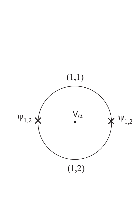
Let us now specialize to the strip with (1,1)(1,1) boundary condition on the left and (1,2)(1,2) boundary condition on the right. The only allowed boundary primary operator/state is ψ1,2\psi_{1,2}. To compute the expectation value of the Liouville field in this state, we need to compute the bulk-boundary three point function ⟨ψ1,2​(y1)​ψ1,2​(y2)​Vα​(z)⟩\langle\psi_{1,2}(y_{1})\psi_{1,2}(y_{2})V_{\alpha}(z)\rangle, with (1,1)(1,1) boundary condition on one segment of the boundary circle and (1,2)(1,2) boundary on the other segment of the circle, between y1y_{1} and y2y_{2}, as shown in Fig. 2.

Refer to caption
Figure 2: Depiction of the bulk-boundary three point function ⟨ψ1,2​(y1)​ψ1,2​(y2)​Vα​(z)⟩\langle\psi_{1,2}(y_{1})\psi_{1,2}(y_{2})V_{\alpha}(z)\rangle with a specific choice of boundary condition.

There are two different ways to factorize ⟨ψ1,2​(y1)​ψ1,2​(y2)​Vα​(z)⟩\langle\psi_{1,2}(y_{1})\psi_{1,2}(y_{2})V_{\alpha}(z)\rangle into the product of a boundary three point function and a bulk-boundary two point function, along channels of (1,1,1,1)(1,1;1,1) boundary type or (1,2,1,2)(1,2;1,2) boundary type. In the first factorization, as shown in Fig. 3, the only boundary primary operator in the channel is the identity operator. We have then

⟨ψ⁡(y1)​ψ​(y2)​Vα​(z)⟩=|z−z¯|−2​Δα​(y1−y2)−2​h​U1,1​(α)​(1−η)α/b​F12​(2​αb,1+b−2,2+2​b−2,η).\langle\psi(y_{1})\psi(y_{2})V_{\alpha}(z)\rangle=|z-\bar{z}|^{-2\Delta_{\alpha}}(y_{1}-y_{2})^{-2h}U_{1,1}(\alpha)(1-\eta)^{\alpha/b}{}_{2}F_{1}({2\alpha\over b},1+b^{-2};2+2b^{-2};\eta)\,. (2.36)
Refer to caption
Figure 3: Factorization of the bulk-boundary three point function along the (1,1,1,1)(1,1;1,1) channel.

In the second factorization, we have the identity operator as well as ψ1,3\psi_{1,3} propagating through the channel, as depicted in Fig. 3, giving

⟨ψ(y1)ψ(y2)Vα(z)⟩=|z−z¯|−2​Δα(y1−y2)−2​h[U1,2(α)(1−η¯)α/b2F1(2​αb,1+b−2;2+2b−2;η¯)\displaystyle\langle\psi(y_{1})\psi(y_{2})V_{\alpha}(z)\rangle=|z-\bar{z}|^{-2\Delta_{\alpha}}(y_{1}-y_{2})^{-2h}\left[U_{1,2}(\alpha)(1-\bar{\eta})^{\alpha/b}{}_{2}F_{1}({2\alpha\over b},1+b^{-2};2+2b^{-2};\bar{\eta})\right. (2.37)
−ie−iπ/b2⟨ψ1,2ψ1,2ψ1,3⟩R1,3(α)(1−η¯)α/bη¯−1−2​b−22F1(−1−2b−2+2​αb,−b−2;−2b−2;η¯)],\displaystyle\left.-ie^{-i\pi/b^{2}}\langle\psi_{1,2}\psi_{1,2}\psi_{1,3}\rangle R_{1,3}(\alpha)(1-\bar{\eta})^{\alpha/b}\bar{\eta}^{-1-2b^{-2}}{}_{2}F_{1}(-1-2b^{-2}+{2\alpha\over b},-b^{-2};-2b^{-2};\bar{\eta})\right],

where η¯\bar{\eta} is the complex conjugate of η\eta. One may also replace η¯\bar{\eta} by η/(η−1)\eta/(\eta-1), and use the property of Gauss hypergeometric functions to rewrite (2.37) in terms of the same functions with argument η\eta. The phase factor −ie−iπ/b2-ie^{-i\pi/b^{2}} in the second term on the RHS is such that in the factorization limit η→i​ϵ\eta\to i\epsilon (σ→π−ϵ\sigma\to\pi-\epsilon), the conformal block corresponding to the ψ1,3\psi_{1,3} is real and positive.

Refer to caption
Figure 4: Factorization of the bulk-boundary three point function along the (1,2,1,2)(1,2;1,2) channel.

One may seem to run into a puzzle here, since the two ways of factorizing the bulk-boundary three point function should give the same result. The resolution is that in fact (2.36) and (2.37) are related by analytic continuation across the branch cut of the hypergeometric function from η=1\eta=1 to infinity. This can be shown using the monodromy of the hypergeometric function around η=1\eta=1, or equivalently

F12​(a,b,c,x+i​ϵ)=e2​π​i​(a+b−c)​F12​(a,b,c,x)\displaystyle{}_{2}F_{1}(a,b;c;x+i\epsilon)=e^{2\pi i(a+b-c)}{}_{2}F_{1}(a,b;c;x) (2.38)
+2​π​i​eπ​i​(a+b−c)​Γ⁡(c)Γ⁡(a+b+1−c)​Γ​(c−a)​Γ​(c−b)​F12​(a,b,a+b+1−c,1−x)\displaystyle+2\pi ie^{\pi i(a+b-c)}{\Gamma(c)\over\Gamma(a+b+1-c)\Gamma(c-a)\Gamma(c-b)}\;{}_{2}F_{1}(a,b;a+b+1-c;1-x)

for real x>1x>1, together with the boundary three point function ⟨ψ1,2​ψ1,2​ψ1,3⟩\langle\psi_{1,2}\psi_{1,2}\psi_{1,3}\rangle which will be explicitly computed below.

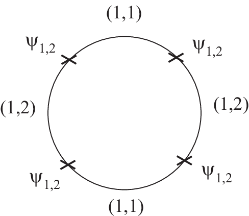
To compute ⟨ψ1,2​ψ1,2​ψ1,3⟩\langle\psi_{1,2}\psi_{1,2}\psi_{1,3}\rangle, we make use of the boundary four point function ⟨ψ1,2​(y1)​ψ1,2​(y2)​ψ1,2​(y3)​ψ1,2​(y4)⟩\langle\psi_{1,2}(y_{1})\psi_{1,2}(y_{2})\psi_{1,2}(y_{3})\psi_{1,2}(y_{4})\rangle, with alternating (1,1)(1,1) and (1,2)(1,2) boundary conditions along the four segments of the boundary circle separated by the boundary operators, see Fig. 5.
Refer to caption
Figure 5: Boundary four point function with alternating boundary conditions.

It is determined by a function 𝒢⁡(ζ){\cal G}(\zeta),

⟨ψ1,2​(y1)​ψ1,2​(y2)​ψ1,2​(y3)​ψ1,2​(y4)⟩\displaystyle\langle\psi_{1,2}(y_{1})\psi_{1,2}(y_{2})\psi_{1,2}(y_{3})\psi_{1,2}(y_{4})\rangle =(y1−y2)−2​h1,2​(y3−y4)−2​h1,2​𝒢​(ζ),\displaystyle=(y_{1}-y_{2})^{-2h_{1,2}}(y_{3}-y_{4})^{-2h_{1,2}}{\cal G}(\zeta), (2.39)
ζ\displaystyle\zeta =(y1−y2)​(y3−y4)(y3−y2)​(y1−y4).\displaystyle={(y_{1}-y_{2})(y_{3}-y_{4})\over(y_{3}-y_{2})(y_{1}-y_{4})}\,.

𝒢⁡(ζ){\cal G}(\zeta) satisfies the same differential equation as that of ℱ⁡(η){\cal F}(\eta), with Δα\Delta_{\alpha} replaced by hh (α→−12​b\alpha\to-{1\over 2b}), η\eta replaced by ζ\zeta. The solutions takes the form

𝒢⁡(ζ)\displaystyle{\cal G}(\zeta) =c1​(1−ζ)−12​b−2​F12​(−b−2,1+b−2,2+2​b−2,ζ)\displaystyle=c_{1}(1-\zeta)^{-{1\over 2}b^{-2}}{}_{2}F_{1}(-b^{-2},1+b^{-2};2+2b^{-2};\zeta) (2.40)
+c2​(1−ζ)−12​b−2​ζ−1−2​b−2​F12​(−1−3​b−2,−b−2,−2​b−2,ζ).\displaystyle+c_{2}(1-\zeta)^{-{1\over 2}b^{-2}}\zeta^{-1-2b^{-2}}{}_{2}F_{1}(-1-3b^{-2},-b^{-2};-2b^{-2};\zeta)\,.

Again, we can factorize it into two boundary three point functions, along either (1,1,1,1)(1,1;1,1) channel (with the only primary being the identity operator) or (1,2,1,2)(1,2;1,2) channel (with primaries 𝟏{\bf 1} and ψ1,3\psi_{1,3}). The two factorizations are shown in Fig. 6.

Refer to caption
Figure 6: The two possible factorizations of the boundary four point function.

The first factorization gives

⟨ψ1,2​(y1)​ψ1,2​(y2)​ψ1,2​(y3)​ψ1,2​(y4)⟩\displaystyle\langle\psi_{1,2}(y_{1})\psi_{1,2}(y_{2})\psi_{1,2}(y_{3})\psi_{1,2}(y_{4})\rangle =(y1−y2)−2​h1,2​(y3−y4)−2​h1,2\displaystyle=(y_{1}-y_{2})^{-2h_{1,2}}(y_{3}-y_{4})^{-2h_{1,2}} (2.41)
×\displaystyle\times (1−ζ)−12​b−2​F12​(−b−2,1+b−2,2+2​b−2,ζ),\displaystyle(1-\zeta)^{-{1\over 2}b^{-2}}{}_{2}F_{1}(-b^{-2},1+b^{-2};2+2b^{-2};\zeta)\,,

while the second factorization gives

⟨ψ1,2​(y1)​ψ1,2​(y2)​ψ1,2​(y3)​ψ1,2​(y4)⟩=C⁡(b)​(y1−y2)−2​h1,2​(y3−y4)−2​h1,2​(1−ζζ)−2​h1,2\displaystyle\langle\psi_{1,2}(y_{1})\psi_{1,2}(y_{2})\psi_{1,2}(y_{3})\psi_{1,2}(y_{4})\rangle=C(b)(y_{1}-y_{2})^{-2h_{1,2}}(y_{3}-y_{4})^{-2h_{1,2}}\left(\frac{1-\zeta}{\zeta}\right)^{-2h_{1,2}} (2.42)
×[ζ−12​b−22F1(−b−2,1+b−2;2+2b−2;1−ζ)\displaystyle\times\left[\zeta^{-{1\over 2}b^{-2}}{}_{2}F_{1}(-b^{-2},1+b^{-2};2+2b^{-2};1-\zeta)\right.
+⟨ψ1,2ψ1,2ψ1,3⟩2ζ−12​b−2(1−ζ)−1−2​b−22F1(−1−3b−2,−b−2;−2b−2;1−ζ)]\displaystyle\left.~~~+\langle\psi_{1,2}\psi_{1,2}\psi_{1,3}\rangle^{2}\,\zeta^{-{1\over 2}b^{-2}}(1-\zeta)^{-1-2b^{-2}}{}_{2}F_{1}(-1-3b^{-2},-b^{-2};-2b^{-2};1-\zeta)\right]

where C⁡(b)=−(2​cos⁡(π​b−2))−1C(b)=-(2\cos(\pi b^{-2}))^{-1} is a normalization factor (which can be determined by matching the two channels as explained below). This nontrivial normalization factor is due to the different boundary conditions on the channels of the two factorizations. In fact, we can identify

C⁡(b)=C1,1​(b)C1,2​(b)C(b)={C_{1,1}(b)\over C_{1,2}(b)} (2.43)

where Cm,n​(b)C_{m,n}(b) stands for the disc amplitude with no insertions and (m,n)(m,n) boundary condition. The forms of (2.41) and (2.42) agree by the identity

F12​(A,B,C,z)\displaystyle{}_{2}F_{1}(A,B;C;z) =Γ⁡(C)​Γ​(C−A−B)Γ⁡(C−A)​Γ​(C−B)​F12​(A,B,A+B+1−C,1−z)\displaystyle={\Gamma(C)\Gamma(C-A-B)\over\Gamma(C-A)\Gamma(C-B)}{}_{2}F_{1}(A,B;A+B+1-C;1-z) (2.44)
+Γ⁡(C)​Γ​(A+B−C)Γ⁡(A)​Γ​(B)​(1−z)C−A−B​F12​(C−A,C−B,1+C−A−B,1−z)\displaystyle+{\Gamma(C)\Gamma(A+B-C)\over\Gamma(A)\Gamma(B)}(1-z)^{C-A-B}{}_{2}F_{1}(C-A,C-B;1+C-A-B;1-z)
=(1−z)C−A−B​F12​(C−A,C−B,C,z).\displaystyle=(1-z)^{C-A-B}{}_{2}F_{1}(C-A,C-B;C;z).

Using this, we then derive the boundary three point function

⟨ψ1,2​ψ1,2​ψ1,3⟩=±[−2​cos⁡(πb2)​Γ⁡(1+2b2)​Γ​(2+2b2)Γ⁡(1+1b2)​Γ​(2+3b2)]12.\langle\psi_{1,2}\psi_{1,2}\psi_{1,3}\rangle=\pm\left[-2\cos({\pi\over b^{2}}){\Gamma(1+{2\over b^{2}})\Gamma(2+{2\over b^{2}})\over\Gamma(1+{1\over b^{2}})\Gamma(2+{3\over b^{2}})}\right]^{1\over 2}. (2.45)

In order to match (2.36) and (2.37) through analytic continuation, as explained above, we need to choose the negative sign in (2.45). Using the results of [8], it follows that

⟨ψ1,2​ψ1,2​ψ1,3⟩​R1,3​(α)U1,1​(α)=−8π​(1+2b2)​sin⁡(2​π​αb)​sin⁡(2​π​α−b−1b)​Γ​(2b2)2​Γ​(1−2​αb)​Γ​(−1−2b2+2​αb)Γ​(1b2)2.{\langle\psi_{1,2}\psi_{1,2}\psi_{1,3}\rangle R_{1,3}(\alpha)\over U_{1,1}(\alpha)}=-{8\over\pi}\left(1+{2\over b^{2}}\right)\sin(2\pi{\alpha\over b})\sin(2\pi{\alpha-b^{-1}\over b}){\Gamma({2\over b^{2}})^{2}\Gamma(1-{2\alpha\over b})\Gamma(-1-{2\over b^{2}}+{2\alpha\over b})\over\Gamma({1\over b^{2}})^{2}}\,. (2.46)

It is also useful to note the identity

U1,2​(α)U1,1​(α)=cos⁡(π⁡(2​αb−1b2))cos⁡(π/b2).{U_{1,2}(\alpha)\over U_{1,1}(\alpha)}={\cos(\pi({2\alpha\over b}-{1\over b^{2}}))\over\cos(\pi/b^{2})}\,. (2.47)

Using (2.46) and (2.47), remarkably, one can check that (2.37) is indeed related to (2.36) by analytic continuation to a different sheet across its branch cut. This also provides a check of the result of [8] for Um,n​(α)U_{m,n}(\alpha) and R1,3​(α)R_{1,3}(\alpha).

The quantum bulk-boundary three-point function can therefore be determined by analytically continuing (2.36) from σ=0\sigma=0 to σ=π\sigma=\pi. In practice, such analytic continuation may be defined by “patching” (2.36) to (2.37) at σ=π/2\sigma=\pi/2, while using the standard definition of the hypergeometric functions with their conventional branch cuts. On the two halves of the strip, we find in the b→0b\to 0 limit, with α/b\alpha/b finite,

⟨ψ1,2|e2​α​ϕ​(σ)|ψ1,2⟩∼U1,1(α)(sin2σ)−2α/b,σ∈(0,π2),\displaystyle\langle\psi_{1,2}|e^{2\alpha\phi(\sigma)}|\psi_{1,2}\rangle\sim U_{1,1}(\alpha)(\sin 2\sigma)^{-2\alpha/b},~~~~\sigma\in(0,{\pi\over 2}), (2.48)
⟨ψ1,2|e2​α​ϕ​(σ)|ψ1,2⟩∼U1,2(α)(sin2σ)−2α/b\displaystyle\langle\psi_{1,2}|e^{2\alpha\phi(\sigma)}|\psi_{1,2}\rangle\sim U_{1,2}(\alpha)(\sin 2\sigma)^{-2\alpha/b}
+⟨ψ1,2​ψ1,2​ψ1,3⟩​R1,3​(α)​(2​sin⁡σ)−1−2​b−2−2​α/b​(cos⁡σ)2​α/b−1,σ∈(π2,π).\displaystyle+\langle\psi_{1,2}\psi_{1,2}\psi_{1,3}\rangle R_{1,3}(\alpha)(2\sin\sigma)^{-1-2b^{-2}-2\alpha/b}(\cos\sigma)^{2\alpha/b-1},~~~~\sigma\in({\pi\over 2},\pi).

We see that for real bb and generic values of α\alpha, in the classical limit the ψ1,3\psi_{1,3} channel dominates for σ>π/2\sigma>\pi/2, and appears to “erase” the right A​d​S2AdS_{2}. The exceptional cases are when the probe bulk operator has α=−nb/2\alpha=-nb/2 for a positive integer nn, and R1,3​(α)R_{1,3}(\alpha) vanishes. In this case the hypergeometric function reduces to elementary functions. For instance, when α=−b/2\alpha=-b/2, we have

⟨ψ1,2|e−b​ϕ​(σ)|ψ1,2⟩=sin⁡2​σ2​(sin⁡σ)32​b2\langle\psi_{1,2}|e^{-b\phi(\sigma)}|\psi_{1,2}\rangle={\sin 2\sigma\over 2}(\sin\sigma)^{{3\over 2}b^{2}} (2.49)

agreeing with the “naive” classical limit of two-fragmented A​d​S2AdS_{2}.

Refer to caption
Figure 7: Plots of the bulk-boundary 3-point function ⟨ψ1,2|Vα​(σ)|ψ1,2⟩\langle\psi_{1,2}|V_{\alpha}(\sigma)|\psi_{1,2}\!\rangle (with α=b\alpha=b) at finite coupling, for bb real (left) and bb imaginary (right), with |b|=0.3|b|=0.3. The dashed line represents the A​d​S2AdS_{2} metric, while the dotted one corresponds to the two-fragmented A​d​S2AdS_{2}. With real bb (left) the asymptotic A​d​S2AdS_{2} boundary condition is respected only at the σ=0\sigma=0 boundary, and the classical limit b→0b\rightarrow 0 produces a single A​d​S2AdS_{2} fragment (the solid line extends to σ=π\sigma=\pi and erases the second A​d​S2AdS_{2}). On the other hand, with imaginary bb (right) the profile is asymptotically A​d​S2AdS_{2} at both boundaries and the limit b→0b\rightarrow 0 gives the two-fragmented A​d​S2AdS_{2} metric.

On the other hand, we can consider b=i​βb=i\beta purely imaginary, and take α\alpha to be purely imaginary as well (or equivalently, Wick rotating the Liouville field ϕ\phi). In the classical limit β→0\beta\to 0 (α/b\alpha/b taken to be real and finite), the identity channel dominates the ψ1,3\psi_{1,3} channel, and we have

⟨ψ1,2|e2​α​ϕ​(σ)|ψ1,2⟩∼U1,1(α)(sin2σ)−2α/b,σ∈(0,π2),\displaystyle\langle\psi_{1,2}|e^{2\alpha\phi(\sigma)}|\psi_{1,2}\rangle\sim U_{1,1}(\alpha)(\sin 2\sigma)^{-2\alpha/b},~~~~\sigma\in(0,{\pi\over 2}), (2.50)
⟨ψ1,2|e2​α​ϕ​(σ)|ψ1,2⟩∼U1,2(α)(sin2σ)−2α/b,σ∈(π2,π),\displaystyle\langle\psi_{1,2}|e^{2\alpha\phi(\sigma)}|\psi_{1,2}\rangle\sim U_{1,2}(\alpha)(\sin 2\sigma)^{-2\alpha/b},~~~~\sigma\in({\pi\over 2},\pi),

i.e. the expectation value of e2​α​ϕ​(σ)e^{2\alpha\phi(\sigma)} scales like (sin2σ)−2α/b(\sin 2\sigma)^{-2\alpha/b} on both halves of the strip, leading to two-fragmented A​d​S2AdS_{2}. Plots of the analytically continued bulk-boundary three point function for real and purely imaginary bb are given in Fig. 7.

We see that near the mid point σ=π/2\sigma=\pi/2 where the two fragmented A​d​S2AdS_{2}’s meet, quantum correction is large despite that the conformal dimension of the probe operator Δα∼α/b≪|c|\Delta_{\alpha}\sim\alpha/b\ll|c|. In particular, the expectation value of Vα​(σ=π/2)V_{\alpha}(\sigma=\pi/2) in the state |ψ1,2⟩|\psi_{1,2}\rangle is given by (using the quadratic transform of F12{}_{2}F_{1})

⟨ψ1,2|e2​α​ϕ​(π/2)|ψ1,2⟩\displaystyle\langle\psi_{1,2}|e^{2\alpha\phi(\pi/2)}|\psi_{1,2}\rangle =F12​(αb,1+b−2−αb,32+b−2,1)\displaystyle={}_{2}F_{1}({\alpha\over b},1+b^{-2}-{\alpha\over b};{3\over 2}+b^{-2};1) (2.51)
=π​Γ​(32+b−2)Γ⁡(12+αb)​Γ​(32+b−2−αb)\displaystyle={\sqrt{\pi}\,\Gamma({3\over 2}+b^{-2})\over\Gamma({1\over 2}+{\alpha\over b})\Gamma({3\over 2}+b^{-2}-{\alpha\over b})}
→{b−2α/bπΓ⁡(12+αb),b→+0,(−b2)−α/bcos⁡(π⁡(αb−b−2))cos⁡(π​b−2)πΓ⁡(12+αb),b→i​0.\displaystyle\to\left\{\begin{array}[]{ll}b^{-2\alpha/b}{\sqrt{\pi}\over\Gamma({1\over 2}+{\alpha\over b})},&b\to+0,\\ (-b^{2})^{-\alpha/b}{\cos(\pi({\alpha\over b}-b^{-2}))\over\cos(\pi b^{-2})}{\sqrt{\pi}\over\Gamma({1\over 2}+{\alpha\over b})},&b\to i0.\end{array}\right.

For instance, for imaginary bb, ⟨ψ1,2|e2​b​ϕ​(σ)|ψ1,2⟩\langle\psi_{1,2}|e^{2b\phi(\sigma)}|\psi_{1,2}\rangle is negative at σ=π/2\sigma=\pi/2, as in figure 7.

Refer to caption
Figure 8: Plots of the expectation value of ϕ⁡(σ)\phi(\sigma) in the ZZ boundary primary |ψ1,2⟩|\psi_{1,2}\rangle, for bb real (left) and bb imaginary (right), with a generic non-integer value of |b−2||b^{-2}|. The dashed line represents the Liouville profile of the A​d​S2AdS_{2} vacuum, while the dotted one corresponds to the two-fragmented A​d​S2AdS_{2}. In the case of imaginary bb, the profile of the Liouville field on the right A​d​S2AdS_{2} is shifted by the constant 2​πb​tan⁡(π/b2){2\pi\over b}\tan(\pi/b^{2}).

It is natural to consider VαV_{\alpha} in the Δα∼α/b→0\Delta_{\alpha}\sim\alpha/b\to 0 limit. We find for bb purely imaginary, in the b→i​0b\to i0 limit,

⟨ψ1,2|ϕ⁡(σ)|ψ1,2⟩\displaystyle\langle\psi_{1,2}|\phi(\sigma)|\psi_{1,2}\rangle =12​∂∂α​⟨ψ1,2|​Vα​(σ)​|ψ1,2⟩|α=0\displaystyle={1\over 2}\left.{\partial\over\partial{\alpha}}\langle\psi_{1,2}|V_{\alpha}(\sigma)|\psi_{1,2}\rangle\right|_{\alpha=0} (2.52)
→{−1b​ln⁡|sin⁡2​σ|+c​o​n​s​t,σ∈(0,π2),−1b​ln⁡|sin⁡2​σ|+2​πb​tan⁡(π/b2)+c​o​n​s​t,σ∈(π2,π),\displaystyle\to\left\{\begin{array}[]{ll}-{1\over b}\ln|\sin 2\sigma|+const,&\sigma\in(0,{\pi\over 2}),\\ -{1\over b}\ln|\sin 2\sigma|+{2\pi\over b}\tan(\pi/b^{2})+const,&\sigma\in({\pi\over 2},\pi),\end{array}\right.

where the overall constant shift can be absorbed into the Liouville cosmological constant. Curiously, the profile of the Liouville field in the two A​d​S2AdS_{2}’s differ by a constant shift 2​πb​tan⁡(π/b2){2\pi\over b}\tan(\pi/b^{2}), coming from the derivative of U1,2​(α)/U1,1​(α)U_{1,2}(\alpha)/U_{1,1}(\alpha) at α=0\alpha=0, which is oscillatory as b→0b\to 0. At the special values b=i/nb={i/\sqrt{n}}, for positive integer nn, this shift is absent and we have a regular semi-classical limit as n→∞n\to\infty. This suggests a quantization of the central charge in Liouville A​d​S2AdS_{2} gravity, c=1+6​Q2=13−6​(n+1n)c=1+6Q^{2}=13-6(n+{1\over n}).

Refer to caption
Figure 9: Plots of the expectation value of ϕ⁡(σ)\phi(\sigma) in the ZZ boundary primary |ψ1,2⟩|\psi_{1,2}\rangle, for bb real (left) and bb imaginary (right), with the integer value of |b−2|=16|b^{-2}|=16. The dashed line represents the Liouville profile of the A​d​S2AdS_{2} vacuum, while the dotted one corresponds to the two-fragmented A​d​S2AdS_{2}.

To summarize the results of this section, we found that:

(1) For real values of bb, in the b→0b\to 0 limit, only one of the two A​d​S2AdS_{2} fragments survives in the quantum theory, and the geometry of the ZZ boundary primary ψ1,2\psi_{1,2} is asymptotically A​d​S2AdS_{2} only near the (1,1)(1,1) boundary, while destroying the A​d​S2AdS_{2} boundary condition on the (1,2)(1,2) boundary. However, the bulk operators V−nb/2V_{-nb/2} for positive integer nn still see the two-fragmented A​d​S2AdS_{2}.

(2) For purely imaginary values of bb, the ZZ boundary primary ψ1,2\psi_{1,2} creates two-fragmented A​d​S2AdS_{2} in the semi-classical limit, which survives in the quantum theory. A regular semi-classical limit also suggests the quantization of the Liouville central charge, b=i/nb=i/\sqrt{n} and c=1+6​Q2=13−6​(n+1n)c=1+6Q^{2}=13-6(n+{1\over n}), where nn is a positive integer.

Perhaps it is worth recalling here that purely imaginary bb is the required choice if one wishes to consistently couple the Liouville sector to a unitary matter CFT, in the semi-classical limit.

2.5 Probing |ψm,n⟩|\psi_{m,n}\rangle with degenerate bulk primaries

In this subsection, we consider the bulk-boundary three point function involving the first degenerate bulk primary V−b/2V_{-b/2} and general ZZ boundary primary ψm,n\psi_{m,n} with (1,1)(1,1) boundary condition on one side of the disc and (m,n)(m,n) boundary condition on the other side,

⟨ψm,n(y1)ψm,n(y2)V−b/2(z,z¯)⟩=|z−z¯|1+32​b2y12−2​hm,nℱ(η).\langle\psi_{m,n}(y_{1})\psi_{m,n}(y_{2})V_{-b/2}(z,\bar{z})\rangle=|z-\bar{z}|^{1+{3\over 2}b^{2}}y_{12}^{-2h_{m,n}}{\cal F}(\eta)\,. (2.53)

The null state at level 2 in the conformal family of V−b/2V_{-b/2} gives rise to a second order differential equation on ℱ⁡(η){\cal F}(\eta). The two independent solutions to the differential equation are conformal blocks corresponding to the factorization on the identity operator and ψ1,3\psi_{1,3}. Since we have chosen the (1,1)(1,1) boundary condition at σ=0\sigma=0, then the factorization through ψ1,3\psi_{1,3} channel is absent as V−b/2V_{-b/2} approaches the left boundary. This fixes the solution to

ℱ⁡(η)=(1−η)n+1+(m+1)​b22​F12​(n+1+(m+1)​b2,1+b2,2+2​b2,η){\cal F}(\eta)=(1-\eta)^{n+1+(m+1)b^{2}\over 2}{}_{2}F_{1}(n+1+(m+1)b^{2},1+b^{2};2+2b^{2};\eta) (2.54)

or in terms of the expectation value of V−b/2V_{-b/2} on the strip,

⟨ψm,n|e−b​ϕ​(σ)|ψm,n⟩\displaystyle\langle\psi_{m,n}|e^{-b\phi(\sigma)}|\psi_{m,n}\rangle =(sin⁡σ)1+32​b2​ei⁡(n+1+(m+1)​b2)​σ​F12​(n+1+(m+1)​b2,1+b2,2+2​b2,1−e2​i​σ)\displaystyle=(\sin\sigma)^{1+{3\over 2}b^{2}}e^{i(n+1+(m+1)b^{2})\sigma}{}_{2}F_{1}(n+1+(m+1)b^{2},1+b^{2};2+2b^{2};1-e^{2i\sigma}) (2.55)
→sin⁡(n​σ)n(b→0),\displaystyle\to{\sin(n\sigma)\over n}~~~~(b\to 0)\,,

confirming the interpretation of ψm,n\psi_{m,n} as nn-fragmented A​d​S2AdS_{2} in the semi-classical limit. Although, we should note that we expect the same subtlety in the case of real bb discussed in the previous section, where generic VαV_{\alpha} will only see one of the nn A​d​S2AdS_{2}’s, the other fragments being “erased” by quantum effects. For purely imaginary bb, however, we expect the nn-fragmented A​d​S2AdS_{2} to survive in the full quantum theory.

3 Interactions of fragmented A​d​S2AdS_{2}

3.1 Boundary three-point functions

Let us denote by ⟨m,n,k⟩\langle m,n,k\rangle the boundary three-point function ⟨ψ1,m​ψ1,n​ψ1,k⟩\langle\psi_{1,m}\psi_{1,n}\psi_{1,k}\rangle with boundary condition of (1,2)(1,2) type between ψ1,m\psi_{1,m} and ψ1,n\psi_{1,n} insertions, (1,n−1)(1,n-1) between ψ1,n\psi_{1,n} and ψ1,k\psi_{1,k}, and (1,m−1)(1,m-1) between ψ1,m\psi_{1,m} and ψ1,k\psi_{1,k}. Note that ⟨m,n,k⟩\langle m,n,k\rangle is not symmetric in n,k,mn,k,m. In the classical limit, however, we have seen that the profile of ψ1,m\psi_{1,m} is not sensitive to the boundary types, provided that the primary ψ1,m\psi_{1,m} is contained in the Hilbert space of the given boundary types. So we expect that the classical limit of ⟨m,n,k⟩\langle m,n,k\rangle to be symmetric in m,n,km,n,k. We will find that this is indeed the case, apart from an oscillating factor. Also note that ⟨m,n,k⟩\langle m,n,k\rangle is nonzero only when |m−n|+1≤k≤m+n−3|m-n|+1\leq k\leq m+n-3 and m+n+k+1∈2​ℤm+n+k+1\in 2{\mathbb{Z}}, due to the selection rule (2.4).

We shall consider the boundary four-point function ⟨2,m,k,n⟩\langle 2,m,k,n\rangle, with boundary condition (1,1,1,m,1,n−1,1,2)(1,1;1,m;1,n-1;1,2) around the boundary circle. It can factorize as

⟨ψ1,2​ψ1,m​ψ1,k​ψ1,n⟩→⟨ψ1,2​ψ1,n​ψ1,n−1⟩​⟨ψ1,n−1​ψ1,2​ψ1,m⟩\langle\psi_{1,2}\psi_{1,m}\psi_{1,k}\psi_{1,n}\rangle\to\langle\psi_{1,2}\psi_{1,n}\psi_{1,n-1}\rangle\langle\psi_{1,n-1}\psi_{1,2}\psi_{1,m}\rangle (3.1)

or as (schematically)

⟨ψ1,2​ψ1,m​ψ1,k​ψ1,n⟩→⟨ψ1,2​ψ1,m​ψ1,m−1⟩​⟨ψ1,m−1​ψ1,n​ψ1,k⟩+⟨ψ1,2​ψ1,m​ψ1,m+1⟩​⟨ψ1,m+1​ψ1,n​ψ1,k⟩.\langle\psi_{1,2}\psi_{1,m}\psi_{1,k}\psi_{1,n}\rangle\to\langle\psi_{1,2}\psi_{1,m}\psi_{1,m-1}\rangle\langle\psi_{1,m-1}\psi_{1,n}\psi_{1,k}\rangle+\langle\psi_{1,2}\psi_{1,m}\psi_{1,m+1}\rangle\langle\psi_{1,m+1}\psi_{1,n}\psi_{1,k}\rangle\,. (3.2)

Writing

⟨ψ1,2​(y1)​ψ1,m​(y2)​ψ1,k​(y4)​ψ1,n​(y3)⟩=(y12​y34)∑hi​(∏1≤i<j≤4yi​j−hi−hj)​ℱ​(η),\langle\psi_{1,2}(y_{1})\psi_{1,m}(y_{2})\psi_{1,k}(y_{4})\psi_{1,n}(y_{3})\rangle=(y_{12}y_{34})^{\sum h_{i}}\left(\prod_{1\leq i<j\leq 4}y_{ij}^{-h_{i}-h_{j}}\right){\cal F}(\eta), (3.3)

where η=y12​y34/y14​y32\eta=y_{12}y_{34}/y_{14}y_{32}, ℱ⁡(η){\cal F}(\eta) obeys the hypergeometric equation coming from the null state in the conformal family of ψ1,2\psi_{1,2}. The general solution is

ℱ(η)=(1−η)(1−n2)​(1+n2​b2)η−1+n+k2+n2+k2−2​m4​b2[C12F1(n−m−k2​b2,1+n+k−m2​b2;−mb2;η)\displaystyle{\cal F}(\eta)=(1-\eta)^{(1-{n\over 2})(1+{n\over 2b^{2}})}\eta^{-1+{n+k\over 2}+{n^{2}+k^{2}-2m\over 4b^{2}}}\left[C_{1}\;{}_{2}F_{1}({n-m-k\over 2b^{2}},1+{n+k-m\over 2b^{2}};-{m\over b^{2}};\eta)\right. (3.4)
+C2η1+mb22F1(1+n+m−k2​b2,2+n+m+k2​b2;2+mb2;η)].\displaystyle\left.+C_{2}\eta^{1+{m\over b^{2}}}\;{}_{2}F_{1}(1+{n+m-k\over 2b^{2}},2+{n+m+k\over 2b^{2}};2+{m\over b^{2}};\eta)\right].

The limit η→0\eta\to 0 corresponds to the factorization through ψm±1\psi_{m\pm 1}, whereas η→1\eta\to 1 corresponds to the factorization though ψn−1\psi_{n-1}. Imposing that there is no factorization through ψn+1\psi_{n+1} (as required by our choice of boundary condition), we find

⟨m+1,2,m⟩​⟨m+1,n,k⟩⟨m−1,2,m⟩​⟨m−1,n,k⟩=C1C2=Γ⁡(2+mb2)​Γ​(k−m−n2​b2)​Γ​(−1−k+m+n2​b2)Γ⁡(−mb2)​Γ​(1+k+m−n2​b2)​Γ​(m−n−k2​b2)\displaystyle{\displaystyle\langle m+1,2,m\rangle\langle m+1,n,k\rangle\over\langle m-1,2,m\rangle\langle m-1,n,k\rangle}={C_{1}\over C_{2}}={\Gamma(2+{m\over b^{2}})\Gamma({k-m-n\over 2b^{2}})\Gamma(-1-{k+m+n\over 2b^{2}})\over\Gamma(-{m\over b^{2}})\Gamma(1+{k+m-n\over 2b^{2}})\Gamma({m-n-k\over 2b^{2}})} (3.5)
=cos⁡((n+k−3​m)​π2​b2)−cos⁡((n+k+m)​π2​b2)cos⁡(k​πb2)−cos⁡((m+n)​πb2)​Γ⁡(1+mb2)​Γ​(2+mb2)​Γ​(1+n+k−m2​b2)Γ⁡(1+k+m−n2​b2)​Γ​(1+m+n−k2​b2)​Γ​(2+k+m+n2​b2).\displaystyle={\cos((n+k-3m){\pi\over 2b^{2}})-\cos((n+k+m){\pi\over 2b^{2}})\over\cos({k\pi\over b^{2}})-\cos({(m+n)\pi\over b^{2}})}{\Gamma(1+{m\over b^{2}})\Gamma(2+{m\over b^{2}})\Gamma(1+{n+k-m\over 2b^{2}})\over\Gamma(1+{k+m-n\over 2b^{2}})\Gamma(1+{m+n-k\over 2b^{2}})\Gamma(2+{k+m+n\over 2b^{2}})}.

Choosing n=2,k=mn=2,k=m, we obtain ⟨m+1,2,m⟩/⟨m−1,2,m⟩\langle m+1,2,m\rangle/\langle m-1,2,m\rangle; then we can further derive ⟨m+1,n,k⟩/⟨m−1,n,k⟩\langle m+1,n,k\rangle/\langle m-1,n,k\rangle. We shall not write the general formula, but focus on the classical limit (b→0b\to 0),

⟨m+1,n,k⟩⟨m−1,n,k⟩∼(oscillatingfactor)×exp[1b2(mlog(4m)+12(m−1)log(m−1)\displaystyle{\displaystyle\langle m+1,n,k\rangle\over\langle m-1,n,k\rangle}\sim(oscillating~factor)\times\exp\left[{1\over b^{2}}(m\log(4m)+{1\over 2}(m-1)\log(m-1)\right. (3.6)
+12​(m+1)​log⁡(m+1)−12​(m+k−n)​log⁡(m+k−n)−12​(m−k+n)​log⁡(m−k+n)\displaystyle\left.+{1\over 2}(m+1)\log(m+1)-{1\over 2}(m+k-n)\log(m+k-n)-{1\over 2}(m-k+n)\log(m-k+n)\right.
+12(−m+k+n)log(−m+k+n)−12(m+k+n)log(m+k+n))+𝒪(1)].\displaystyle\left.+{1\over 2}(-m+k+n)\log(-m+k+n)-{1\over 2}(m+k+n)\log(m+k+n))+{\cal O}(1)\right].

Iterating this relation, we find

⟨1+x,1+y,1+z⟩⟨−1+x,−1+y,−1+z⟩∼(oscillatingfactor)×exp[1b2(xlog(4x)+12(x−1)log(x−1)\displaystyle{\displaystyle\langle 1+x,1+y,1+z\rangle\over\langle-1+x,-1+y,-1+z\rangle}\sim(oscillating~factor)\times\exp\left[{1\over b^{2}}(x\log(4x)+{1\over 2}(x-1)\log(x-1)\right. (3.7)
+12​(x+1)​log⁡(x+1)+y​log⁡(4​y)+12​(y−1)​log⁡(y−1)+12​(y+1)​log⁡(y+1)\displaystyle\left.+{1\over 2}(x+1)\log(x+1)+y\log(4y)+{1\over 2}(y-1)\log(y-1)+{1\over 2}(y+1)\log(y+1)\right.
+z​log⁡(4​z)+12​(z−1)​log⁡(z−1)+12​(z+1)​log⁡(z+1)\displaystyle\left.+z\log(4z)+{1\over 2}(z-1)\log(z-1)+{1\over 2}(z+1)\log(z+1)\right.
−12​(x+y−z)​log⁡(x+y−z)−12​(x−y+z)​log⁡(x−y+z)\displaystyle\left.-{1\over 2}(x+y-z)\log(x+y-z)-{1\over 2}(x-y+z)\log(x-y+z)\right.
−12​(−x+y+z)​log⁡(−x+y+z)−12​(x+y+z)​log⁡(x+y+z)\displaystyle\left.-{1\over 2}(-x+y+z)\log(-x+y+z)-{1\over 2}(x+y+z)\log(x+y+z)\right.
−12(x+y+z−2)log(x+y+z−2)−12(x+y+z+2)log(x+y+z+2))+𝒪(1)].\displaystyle\left.-{1\over 2}(x+y+z-2)\log(x+y+z-2)-{1\over 2}(x+y+z+2)\log(x+y+z+2))+{\cal O}(1)\right].

This expression is particularly interesting because, as we will show in section 3.4 below, an analytic continuation to non-integer x,y,zx,y,z can be matched against the geodesic approximation of three point particles in A​d​S2AdS_{2}.

We can also give a closed form expression in the limit x,y,z≫1x,y,z\gg 1, corresponding to the scattering of A​d​S2AdS_{2}’s with many fragments. In this case, we get

⟨x,y,z⟩∼exp[1b2(x2logx+y2logy+z2logz−(x+y−z)24log(x+y−z)\displaystyle\langle x,y,z\rangle\sim\exp\left[{1\over b^{2}}(x^{2}\log x+y^{2}\log y+z^{2}\log z-{(x+y-z)^{2}\over 4}\log(x+y-z)\right. (3.8)
−(x−y+z)24log(x−y+z)−(−x+y+z)24log(−x+y+z)−(x+y+z)24log(x+y+z))].\displaystyle\left.-{(x-y+z)^{2}\over 4}\log(x-y+z)-{(-x+y+z)^{2}\over 4}\log(-x+y+z)-{(x+y+z)^{2}\over 4}\log(x+y+z))\right].

3.2 Bulk-boundary four-point functions

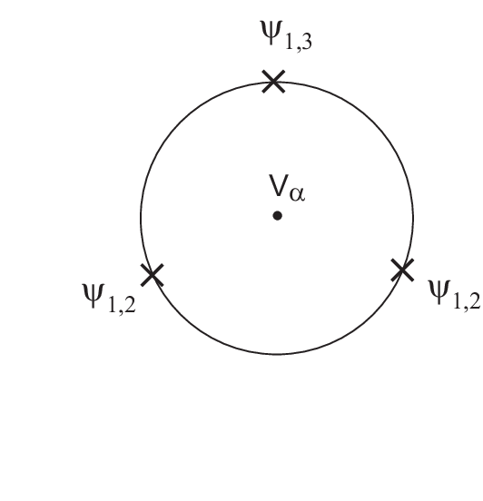
In this section we study the disc bulk-boundary four-point function ⟨ψ1,2​(y1)​ψ1,2​(y2)​ψ1,3​(y3)​Vα​(z,z¯)⟩\langle\psi_{1,2}(y_{1})\psi_{1,2}(y_{2})\psi_{1,3}(y_{3})V_{\alpha}(z,\bar{z})\rangle, see Fig. 10. The choice of boundary type is not important for now, since we will be interested in the classical limit of this correlation function.
Refer to caption
Figure 10: The bulk-boundary four point function.

By conformal invariance, this four-point function takes the form

⟨ψ1,2​(y1)​ψ1,2​(y2)​ψ1,3​(y3)​Vα​(z,z¯)⟩=|z−z¯|−2​Δα​y12−2​h1,2+h1,3​(y13​y23)−h1,3​ℱ​(η,η¯)\langle\psi_{1,2}(y_{1})\psi_{1,2}(y_{2})\psi_{1,3}(y_{3})V_{\alpha}(z,\bar{z})\rangle=|z-\bar{z}|^{-2\Delta_{\alpha}}y_{12}^{-2h_{1,2}+h_{1,3}}(y_{13}y_{23})^{-h_{1,3}}{\cal F}(\eta,\bar{\eta}) (3.9)

where

η=(z−y1)​y23(z−y3)​y21,η¯=(z¯−y1)​y23(z¯−y3)​y21.\eta={(z-y_{1})y_{23}\over(z-y_{3})y_{21}},~~~~\bar{\eta}={(\bar{z}-y_{1})y_{23}\over(\bar{z}-y_{3})y_{21}}. (3.10)

We can use the S​L​(2,ℝ)SL(2,\mathbb{R}) symmetry to fix for example y1=0,y2=1y_{1}=0,y_{2}=1 and y3=∞y_{3}=\infty. Then η\eta and η¯\bar{\eta} simply coincide with the coordinates zz and z¯\bar{z} parameterizing the position of the “probe” bulk primary Vα​(z,z¯)V_{\alpha}(z,\bar{z}).

The constraining equation from the level 2 null state in the conformal family of ψ1,2​(y1)\psi_{1,2}(y_{1}) reduces to a second order differential equation on ℱ{\cal F},

Δα​(η−η¯)2​ℱ+η¯2​η​(η−1)​(2​(1+b2)​η+1)​∂ηℱ+η2​η¯​(η¯−1)​(2​(1+b2)​η¯+1)​∂η¯ℱ\displaystyle\Delta_{\alpha}(\eta-\bar{\eta})^{2}{\cal F}+\bar{\eta}^{2}\eta(\eta-1)(2(1+b^{2})\eta+1)\partial_{\eta}{\cal F}+\eta^{2}\bar{\eta}(\bar{\eta}-1)(2(1+b^{2})\bar{\eta}+1)\partial_{\bar{\eta}}{\cal F} (3.11)
+b2​η2​η¯2​[(η−1)2​∂η2ℱ+(η¯−1)2​∂η¯2ℱ+2​|η−1|2​∂η∂η¯ℱ]=0.\displaystyle+b^{2}\eta^{2}\bar{\eta}^{2}\left[(\eta-1)^{2}\partial_{\eta}^{2}{\cal F}+(\bar{\eta}-1)^{2}\partial_{\bar{\eta}}^{2}{\cal F}+2|\eta-1|^{2}\partial_{\eta}\partial_{\bar{\eta}}{\cal F}\right]=0\,.

In the classical limit b→0b\rightarrow 0 (with αb\alpha\over b fixed), this reduces to the first order equation

Δα​(η−η¯)2​ℱc​l+η¯2​η​(η−1)​(2​η+1)​∂ηℱc​l+η2​η¯​(η¯−1)​(2​η¯+1)​∂η¯ℱc​l=0.\Delta_{\alpha}(\eta-\bar{\eta})^{2}{\cal F}^{cl}+\bar{\eta}^{2}\eta(\eta-1)(2\eta+1)\partial_{\eta}{\cal F}^{cl}+\eta^{2}\bar{\eta}(\bar{\eta}-1)(2\bar{\eta}+1)\partial_{\bar{\eta}}{\cal F}^{cl}=0\,. (3.12)

Similarly, there is another equation coming from ψ1,2​(y2)\psi_{1,2}(y_{2}), which is identical to the above equation with ℱ⁡(η,η¯){\cal F}(\eta,\bar{\eta}) replaced by ℱ⁡(1−η,1−η¯){\cal F}(1-\eta,1-\bar{\eta}). The solution to this pair of equations is (up to a normalization constant)

ℱc​l​(η,η¯)=[|η|2​|1−η|2​(2​η2+2​η¯2+2​|η|2−3​η−3​η¯)−2]Δα.{\cal F}^{cl}(\eta,\bar{\eta})=\left[|\eta|^{2}|1-\eta|^{2}(2\eta^{2}+2\bar{\eta}^{2}+2|\eta|^{2}-3\eta-3\bar{\eta})^{-2}\right]^{\Delta_{\alpha}}. (3.13)

This means that if the classical limit of the three-point function ⟨ψ1,2​(y1)​ψ1,2​(y2)​ψ1,3​(y3)⟩\langle\psi_{1,2}(y_{1})\psi_{1,2}(y_{2})\psi_{1,3}(y_{3})\rangle is dominated by an instanton solution, the solution has Liouville profile

⟨e2​α​ϕ⟩i​n​s​t=|z−z¯|−2α/b[|z|2|1−z|2(2z2+2z¯2+2|z|2−3z−3z¯)−2]α/b.\langle e^{2\alpha\phi}\rangle_{inst}=|z-\bar{z}|^{-2\alpha/b}\left[|z|^{2}|1-z|^{2}(2z^{2}+2\bar{z}^{2}+2|z|^{2}-3z-3\bar{z})^{-2}\right]^{\alpha/b}\,. (3.14)

The instanton solution has “physical” metric (we fix the overall normalization to agree with the conventions of ZZ)

e2​b​ϕ​d​z​d​z¯=36​|z|2​|1−z|2​d​z​d​z¯π​b2​|z−z¯|2​(2​z2+2​z¯2+2​|z|2−3​z−3​z¯)2.e^{2b\phi}dzd\bar{z}={36|z|^{2}|1-z|^{2}dzd\bar{z}\over\pi b^{2}|z-\bar{z}|^{2}(2z^{2}+2\bar{z}^{2}+2|z|^{2}-3z-3\bar{z})^{2}}. (3.15)

This is indeed a solution to Liouville equation, and corresponds to three Poincaré discs patched together, depicted schematically in Fig. 11.

Refer to caption
Figure 11: Schematic depiction of the classical solution (3.15), corresponding to three Poincaré discs patched together along the dashed lines.

In the upper half plane coordinate z=x+i​yz=x+iy, the three disconnected A​d​S2AdS_{2}’s are glued along the two curves

y=3​x​(x−1),x<0​or​x>1.y=\sqrt{3x(x-1)},~~~~x<0~{\rm or}~x>1. (3.16)

A contour plot of the classical solution (3.15) in the upper half plane coordinates, showing the curves (3.16) is shown in Fig. 12.

Refer to caption
Figure 12: Contour plot of the solution (3.15) in the upper half plane coordinates. The points x=0x=0 and x=1x=1 on the real axis correspond to the insertions of the two ψ1,2\psi_{1,2} operators. The “fragmentation lines” are described by eq. (3.16).

It is also interesting to visualize the solution in the strip coordinates defined by z=ei​σ+τz=e^{i\sigma+\tau}. The corresponding plot is shown in Fig. 13.

It is actually not difficult to obtain the classical instanton profile for more general boundary three point functions. Consider for example the four point function ⟨ψ1,3​(y1)​ψ1,3​(y2)​ψ1,3​(y3)​Vα​(z,z¯)⟩\langle\psi_{1,3}(y_{1})\psi_{1,3}(y_{2})\psi_{1,3}(y_{3})V_{\alpha}(z,\bar{z})\rangle. Again, by conformal invariance we can write

⟨ψ1,3​(y1)​ψ1,3​(y2)​ψ1,3​(y3)​Vα​(z,z¯)⟩=|z−z¯|−2​Δα​(y12​y13​y23)−h1,3​ℱ333​(η,η¯)\langle\psi_{1,3}(y_{1})\psi_{1,3}(y_{2})\psi_{1,3}(y_{3})V_{\alpha}(z,\bar{z})\rangle=|z-\bar{z}|^{-2\Delta_{\alpha}}(y_{12}y_{13}y_{23})^{-h_{1,3}}{\cal F}_{333}(\eta,\bar{\eta}) (3.17)

where η\eta and η¯\bar{\eta} are defined as above. The constraining equation from the null state in the conformal family of ψ1,3​(y1)\psi_{1,3}(y_{1}), see eq. (2.19), reduces in the classical limit to the first order differential equation

2​Δα​(η−η¯)2​(|η|2−η−η¯)​ℱ333c​l+η​η¯3​(η2−1)​(2​η−1)​∂ηℱ333c​l+η¯​η3​(η¯2−1)​(2​η¯−1)​∂η¯ℱ333c​l=0,2\Delta_{\alpha}(\eta-\bar{\eta})^{2}(|\eta|^{2}-\eta-\bar{\eta}){\cal F}^{cl}_{333}+\eta\bar{\eta}^{3}(\eta^{2}-1)(2\eta-1)\partial_{\eta}{\cal F}^{cl}_{333}+\bar{\eta}\eta^{3}(\bar{\eta}^{2}-1)(2\bar{\eta}-1)\partial_{\bar{\eta}}{\cal F}^{cl}_{333}=0\,, (3.18)

and as before there is a similar equation coming from ψ1,3​(y2)\psi_{1,3}(y_{2}). The solution to this couple of first order differential equations (up to an overall constant) turns out to be

ℱ333c​l​(η,η¯)=[|η|2​|1−η|2(η3+η¯3−2​(η2+η¯2)​(|η|2+1)+|η|2​(5​η+5​η¯−2​|η|2−2))2]Δα,{\cal F}^{cl}_{333}(\eta,\bar{\eta})=\left[\frac{|\eta|^{2}|1-\eta|^{2}}{\left(\eta^{3}+\bar{\eta}^{3}-2(\eta^{2}+\bar{\eta}^{2})(|\eta|^{2}+1)+|\eta|^{2}(5\eta+5\bar{\eta}-2|\eta|^{2}-2)\right)^{2}}\right]^{\Delta_{\alpha}}\,, (3.19)

and the physical instanton metric (Δα=1\Delta_{\alpha}=1) corresponding to the three point function ⟨ψ1,3​ψ1,3​ψ1,3⟩\langle\psi_{1,3}\psi_{1,3}\psi_{1,3}\rangle is therefore

e2​b​ϕ​d​z​d​z¯=36​|z|2​|1−z|2​d​z​d​z¯π​b2​|z−z¯|2​(z3+z¯3−2​(z2+z¯2)​(|z|2+1)+|z|2​(5​z+5​z¯−2​|z|2−2))2.e^{2b\phi}dzd\bar{z}={36|z|^{2}|1-z|^{2}dzd\bar{z}\over\pi b^{2}|z-\bar{z}|^{2}\left(z^{3}+\bar{z}^{3}-2(z^{2}+\bar{z}^{2})(|z|^{2}+1)+|z|^{2}(5z+5\bar{z}-2|z|^{2}-2)\right)^{2}}. (3.20)

One can verify that this is a solution to Liouville equation, and as expected corresponds to four copies of the Poincaré disc patched together.

Refer to caption
Figure 13: Strip coordinates plot of the classical Liouville profile corresponding to the boundary three point function <ψ1,2​ψ1,2​ψ1,3><\psi_{1,2}\psi_{1,2}\psi_{1,3}>. The strip τ∈ℝ\tau\in\mathbb{R}, 0≤σ≤π\,0\leq\sigma\leq\pi fragments into three disconnected pieces.

3.3 Instantons interpolating fragmented A​d​S2AdS_{2}’s

It is instructive to write the above solutions in the general form

e2​b​ϕ=1π​b2​∂A⁡(z)​∂¯​B​(z¯)(1−A⁡(z)​B​(z¯))2,e^{2b\phi}=\frac{1}{\pi b^{2}}\frac{\partial A(z)\bar{\partial}B(\bar{z})}{(1-A(z)B(\bar{z}))^{2}}\,, (3.21)

which is in fact the most general solution of Liouville equation

∂∂¯​ϕ−π​b​e2​b​ϕ=0.\partial\bar{\partial}\phi-\pi be^{2b\phi}=0\,. (3.22)

For example, the regular A​d​S2AdS_{2} solution corresponds to B⁡(z¯)=1/A⁡(z¯)B(\bar{z})=1/A(\bar{z}) and A⁡(z)=zA(z)=z, while the nn-fragmented solution has A⁡(z)=znA(z)=z^{n}. In fact, this is perhaps the fastest way to see that the stress tensor for the nn-fragmented A​d​S2AdS_{2} agrees with the conformal dimension of the operator ψ1,n\psi_{1,n} (one simply looks at the Schwartzian derivative of the conformal transformation w=znw=z^{n}).

Going back to the “instanton” solutions (3.15),(3.20) found above, one can see that they take indeed the form (3.21) (still with B⁡(z¯)=1/A⁡(z¯)B(\bar{z})=1/A(\bar{z}), which ensures that the metric is real). By direct calculation one finds that ∂A⁡(z)=z⁡(z−1)\partial A(z)=z(z-1) for the ⟨ψ1,2​ψ1,2​ψ1,3⟩\langle\psi_{1,2}\psi_{1,2}\psi_{1,3}\rangle and ∂A⁡(z)=z2​(z−1)2(z−12)2\partial A(z)=\frac{z^{2}(z-1)^{2}}{(z-\frac{1}{2})^{2}} for the ⟨ψ1,3​ψ1,3​ψ1,3⟩\langle\psi_{1,3}\psi_{1,3}\psi_{1,3}\rangle case. Motivated by this, we conjecture that the general instanton solution corresponding to the three point function ⟨ψ1,n​(0)​ψ1,m​(1)​ψ1,k​(∞)⟩\langle\psi_{1,n}(0)\psi_{1,m}(1)\psi_{1,k}(\infty)\rangle is given by 22 2 The metric (3.21) with B=1/A¯B=1/\bar{A} is invariant under the S​L​(2,ℝ)SL(2,\mathbb{R}) transformation A→(a​A+b)/(c​A+d)A\rightarrow(aA+b)/(cA+d), ∂A→∂A/(c​A+d)2\partial A\rightarrow\partial A/(cA+d)^{2}. One can reach the standard form (3.23) by applying such S​L​(2,ℝ)SL(2,\mathbb{R}) transformation.

∂A⁡(z)=zn−1​(z−1)m−1P​(z)2,\partial A(z)=\frac{z^{n-1}(z-1)^{m-1}}{P(z)^{2}}\,, (3.23)

where P⁡(z)P(z) is a (n+m−k−1)/2(n+m-k-1)/2-degree polynomial with distinct roots (to be determined below), namely P⁡(z)=∏i=1(n+m−k−1)/2(z−zi)P(z)=\prod_{i=1}^{(n+m-k-1)/2}(z-z_{i}). Note that (n+m−k−1)/2(n+m-k-1)/2 is an integer as implied by the three point function selection rules. The conjecture is motivated as follows. First, the degree of the zeroes at z=0z=0 and z=1z=1 and of the pole at z=∞z=\infty are fixed by demanding that near those points the metric looks respectively like the nn-fragmented, the mm-fragmented and the kk-fragemented A​d​S2AdS_{2}. Furthermore, the fact that P⁡(z)P(z) has distinct roots and the denominator of (3.23) is P​(z)2P(z)^{2} follows by requiring that near each of the ziz_{i} the metric looks like the regular A​d​S2AdS_{2}. To see this, consider for simplicity ∂A⁡(z)∼1(z−z0)s\partial A(z)\sim\frac{1}{(z-z_{0})^{s}} near z=z0z=z_{0}. Then writing z=z0+r​ei​θz=z_{0}+re^{i\theta}, the metric close to z0z_{0} takes the form

d​s2∼(d​r/r)2+d​θ2sin2⁡((s−1)​θ),ds^{2}\sim\frac{(dr/r)^{2}+d\theta^{2}}{\sin^{2}((s-1)\theta)}\,,

so that we have to choose s=2s=2 as claimed. Finally, whe have to specify the position of the roots ziz_{i} of P⁡(z)P(z). If we insist that A⁡(z)A(z) has to be a rational function, which seems to be a natural assumption, then the roots can be determined by requiring that the poles at z=ziz=z_{i} have vanishing residue, namely

dd​z​[(z−zi)2​∂A⁡(z)]|z=zi=0i=1,⋯,n+m−k−12.\frac{d}{dz}\left[(z-z_{i})^{2}\partial A(z)\right]|_{z=z_{i}}=0\,~~~~~~i=1,\cdots,\frac{n+m-k-1}{2}\,. (3.24)

It is easy to verify that the above solutions for ⟨ψ1,2​ψ1,2​ψ1,3⟩\langle\psi_{1,2}\psi_{1,2}\psi_{1,3}\rangle and ⟨ψ1,3​ψ1,3​ψ1,3⟩\langle\psi_{1,3}\psi_{1,3}\psi_{1,3}\rangle satisfy the conjecture (3.23). By directly solving for the classical limit of the bulk-boundary four point function as described above, we have also successfully checked the conjecture on a few other explicit examples such as ⟨ψ1,2​ψ1,3​ψ1,4⟩\langle\psi_{1,2}\psi_{1,3}\psi_{1,4}\rangle and ⟨ψ1,3​ψ1,3​ψ1,5⟩\langle\psi_{1,3}\psi_{1,3}\psi_{1,5}\rangle, which respectively have ∂A⁡(z)=z​(z−1)2\partial A(z)=z(z-1)^{2} and ∂A⁡(z)=z2​(z−1)2\partial A(z)=z^{2}(z-1)^{2}. Other tests of (3.23),(3.24) come from these known examples by applying an inversion z→1/zz\rightarrow 1/z to map the origin to infinity. For example, one finds that the solution for ⟨ψ1,3​(0)​ψ1,2​(1)​ψ1,2​(∞)⟩\langle\psi_{1,3}(0)\psi_{1,2}(1)\psi_{1,2}(\infty)\rangle has ∂A⁡(z)=z2​(z−1)(z−2/3)2\partial A(z)=\frac{z^{2}(z-1)}{(z-2/3)^{2}} in agreement with the conjecture. A further check comes from ⟨ψ1,5​(0)​ψ1,3​(1)​ψ1,3​(∞)⟩\langle\psi_{1,5}(0)\psi_{1,3}(1)\psi_{1,3}(\infty)\rangle, which turns out to be given by ∂A⁡(z)=z4​(z−1)2(z−z1)2​(z−z¯1)2\partial A(z)=\frac{z^{4}(z-1)^{2}}{(z-z_{1})^{2}(z-\bar{z}_{1})^{2}} with z1=120​(15+i​15)z_{1}=\frac{1}{20}(15+i\sqrt{15}), as predicted by (3.23),(3.24)(\ref{Aprime}),(\ref{roots}).

3.4 Comparison with the geodesic approximation

Consider the classical limit b→0b\rightarrow 0 of the boundary three point function, for example eq. (2.45). In this limit one gets

⟨ψ1,2ψ1,2ψ1,3⟩∼±2​2334(−cosπb2)12e−12​b2​ln⁡2716,realb→0,\displaystyle\langle\psi_{1,2}\psi_{1,2}\psi_{1,3}\rangle\sim\pm\frac{2\sqrt{2}}{3^{\frac{3}{4}}}\left(-\cos\frac{\pi}{b^{2}}\right)^{\frac{1}{2}}\,e^{-\frac{1}{2b^{2}}\ln\frac{27}{16}},~~~~{\rm real}~b\to 0, (3.25)
⟨ψ1,2ψ1,2ψ1,3⟩∼±2334(−1+2​cos⁡2​πb2cos⁡πb2)12e−12​b2​ln⁡2716,imaginaryb→0.\displaystyle\langle\psi_{1,2}\psi_{1,2}\psi_{1,3}\rangle\sim\pm\frac{\sqrt{2}}{3^{\frac{3}{4}}}\left(-{1+2\cos\frac{2\pi}{b^{2}}\over\cos\frac{\pi}{b^{2}}}\right)^{\frac{1}{2}}\,e^{-\frac{1}{2b^{2}}\ln\frac{27}{16}},~~~~{\rm imaginary}~b\to 0.

The exponential term suggests that it should be possible to obtain this result by a semiclassical gravity calculation.33 3 Curiously, for a special set of “quantized” values of bb, namely b−2=nb^{-2}=n being an odd integer, the oscillatory factor on the RHS of (3.25) is a constant independent nn. Namely one should evaluate the regularized action on the “instanton” solution, i.e. the classical Liouville profile (3.15), corresponding to the insertion of the three boundary primary operators, which was obtained in section 3.2. In this section we present a different calculation based on point particles moving along geodesics in A​d​S2AdS_{2}, which interestingly matches a particular analytic continuation of the boundary three point function discussed in Section 3.1.

Consider three point particles of masses m1,m2,m3m_{1},m_{2},m_{3} starting off at the boundary of the disk and moving along geodesics until they meet at one point in the interior. The geodesic approximation is expected to be valid when the mass of the particles are large compared to the A​d​SAdS scale, and the gravity coupling is weak, i.e. in the limit 1≪mi≪1/b21\ll m_{i}\ll 1/b^{2} (in A​d​SAdS units). Mapping the problem to the upper half plane, we can place the particles with masses m1m_{1} and m2m_{2} on the real line (separated say by a distance LL), and the particle with mass m3m_{3} at i​∞i\infty. The particles m1m_{1} and m2m_{2} move along circles and m3m_{3} along a straight line, until the geodesics meet at a certain height hh, as shown in Fig. 14.

Refer to caption
Figure 14: Three point particles of masses m1,m2,m3m_{1},m_{2},m_{3} moving along geodesics in the Poincarè half plane.

Using as variables the final angular position θ1\theta_{1} and θ2\theta_{2} of the circular geodesics, the total action for the system reads

S=m1​∫ϵR1θ1d​θsin⁡θ+m2​∫ϵR2θ2d​θsin⁡θ+m3​ln⁡Λh,S=m_{1}\int_{\frac{\epsilon}{R_{1}}}^{\theta_{1}}\frac{d\theta}{\sin\theta}+m_{2}\int_{\frac{\epsilon}{R_{2}}}^{\theta_{2}}\frac{d\theta}{\sin\theta}+m_{3}\ln\frac{\Lambda}{h}\,, (3.26)

where we have introduced cutoffs ϵ→0\epsilon\rightarrow 0 and Λ→∞\Lambda\rightarrow\infty. The geometry implies

h⁡(θ1,θ2)=Ltan⁡θ12+tan⁡θ22R1,2=hsin⁡θ1,2.h(\theta_{1},\theta_{2})=\frac{L}{\tan\frac{\theta_{1}}{2}+\tan\frac{\theta_{2}}{2}}\,~~~~~R_{1,2}=\frac{h}{\sin\theta_{1,2}}\,. (3.27)

Then one gets

S=\displaystyle S= (m1+m2−m3)​ln⁡h−m1​ln⁡cos2⁡θ12−m2​ln⁡cos2⁡θ22\displaystyle(m_{1}+m_{2}-m_{3})\ln h-m_{1}\ln\cos^{2}\frac{\theta_{1}}{2}-m_{2}\ln\cos^{2}\frac{\theta_{2}}{2} (3.28)
−(m1+m2)​ln⁡ϵ+m3​ln⁡Λ.\displaystyle-(m_{1}+m_{2})\ln\epsilon+m_{3}\ln\Lambda\,.

It is not difficult to extremize this action with respect to θ1\theta_{1} and θ2\theta_{2} for general m1,m2,m3m_{1},m_{2},m_{3}. The solution turns out to be

tan2⁡θ12=m22−(m1−m3)2(m1+m3)2−m22,tan2⁡θ22=m12−(m2−m3)2(m2+m3)2−m12.\tan^{2}\frac{\theta_{1}}{2}=\frac{m_{2}^{2}-(m_{1}-m_{3})^{2}}{(m_{1}+m_{3})^{2}-m_{2}^{2}}\,,~~~~~~~~~\tan^{2}\frac{\theta_{2}}{2}=\frac{m_{1}^{2}-(m_{2}-m_{3})^{2}}{(m_{2}+m_{3})^{2}-m_{1}^{2}}\,. (3.29)

Plugging back into (3.28) and removing the divergencies, one finds the following general formula for the regularized action

Sr​e​g=1b2[∑i=13milog(2mi)−12(m1+m2−m3)log(m1+m2−m3)\displaystyle S_{reg}={1\over b^{2}}\left[\sum_{i=1}^{3}m_{i}\log(2m_{i})-{1\over 2}(m_{1}+m_{2}-m_{3})\log(m_{1}+m_{2}-m_{3})\right. (3.30)
−12​(m1−m2+m3)​log⁡(m1−m2+m3)−12​(−m1+m2+m3)​log⁡(−m1+m2+m3)\displaystyle\left.-{1\over 2}(m_{1}-m_{2}+m_{3})\log(m_{1}-m_{2}+m_{3})-{1\over 2}(-m_{1}+m_{2}+m_{3})\log(-m_{1}+m_{2}+m_{3})\right.
−12(m1+m2+m3)log(m1+m2+m3)].\displaystyle\left.-{1\over 2}(m_{1}+m_{2}+m_{3})\log(m_{1}+m_{2}+m_{3})\right]\,.

This expression matches the classical limit of the boundary three point function (3.7) if we take the masses to be m1=−x/b2,m2=−y/b2,m3=−z/b2m_{1}=-x/b^{2},m_{2}=-y/b^{2},m_{3}=-z/b^{2}, with small real x,y,zx,y,z. Note that the conformal dimension corresponding to a scalar of mass mm is h=12+12​1+m2h=\frac{1}{2}+\frac{1}{2}\sqrt{1+m^{2}} (where mm is expressed in units of the A​d​SAdS radius) [2]. In our limit h∼m2h\sim\frac{m}{2}, consistently with the dimension Δ1,1+x∼−x2​b2\Delta_{1,1+x}\sim-\frac{x}{2b^{2}} of the “analytically continued” operator ψ1,1+x\psi_{1,1+x}.

Acknowledgments

We are grateful to D. Gaiotto, G. Moore, A. Pakman and D. Shih for useful discussions, and especially to A. Strominger for collaborations at the initial stage of this work and on related topics. X.Y. would like to thank Tata Insititute of Fundamental Research and the organizers of the Monsoon Workshop on String Theory for hospitality during the completion of this work. The work of S.G. is supported in part by the Center for the Fundamental Laws of Nature at Harvard University and by NSF grants PHY-024482 and DMS-0244464. The work of X.Y. is supported by a Junior Fellowship from the Harvard Society of Fellows.

References

  • [1] P. H. Ginsparg and G. W. Moore, “Lectures on 2-D gravity and 2-D string theory,” arXiv:hep-th/9304011.
  • [2] A. Strominger, “AdS(2) quantum gravity and string theory,” JHEP 9901, 007 (1999) [arXiv:hep-th/9809027].
  • [3] J. M. Maldacena, J. Michelson and A. Strominger, “Anti-de Sitter fragmentation,” JHEP 9902, 011 (1999) [arXiv:hep-th/9812073].
  • [4] A. Strominger, “A matrix model for AdS(2),” JHEP 0403, 066 (2004) [arXiv:hep-th/0312194].
  • [5] T. Hartman and A. Strominger, “Central Charge for A​d​S2AdS_{2} Quantum Gravity,” JHEP 0904, 026 (2009) [arXiv:0803.3621 [hep-th]].
  • [6] A. Sen, “Quantum Entropy Function from AdS(2)/CFT(1) Correspondence,” arXiv:0809.3304 [hep-th].
  • [7] A. Sen, “Entropy Function and AdS(2)/CFT(1) Correspondence,” JHEP 0811, 075 (2008) [arXiv:0805.0095 [hep-th]].
  • [8] A. B. Zamolodchikov and A. B. Zamolodchikov, “Liouville field theory on a pseudosphere,” arXiv:hep-th/0101152.
  • [9] V. Fateev, A. B. Zamolodchikov and A. B. Zamolodchikov, “Boundary Liouville field theory. I: Boundary state and boundary two-point function,” arXiv:hep-th/0001012.
  • [10] N. Seiberg, “Notes on quantum Liouville theory and quantum gravity,” Prog. Theor. Phys. Suppl. 102, 319 (1990).
  • [11] Y. Nakayama, “Liouville field theory: A decade after the revolution,” Int. J. Mod. Phys. A 19, 2771 (2004) [arXiv:hep-th/0402009].
  • [12] A. M. Polyakov, “Quantum geometry of bosonic strings,” Phys. Lett. B 103, 207 (1981).
  • [13] E. D’Hoker and R. Jackiw, “Liouville Field Theory,” Phys. Rev. D 26, 3517 (1982).
  • [14] E. D’Hoker, D. Z. Freedman and R. Jackiw, “SO(2,1) Invariant Quantization Of The Liouville Theory,” Phys. Rev. D 28, 2583 (1983).
  • [15] N. M. Temme, “Large parameter cases of the Gauss hypergeometric function,” Journal of Computational and Applied Mathematics 153 (2003), 441-462.
  • [16] P. Di Francesco, P. Mathieu and D. Senechal, “Conformal Field Theory,” New York, USA: Springer (1997) 890 p