LLE with low-dimensional neighborhood representation
Abstract
The local linear embedding algorithm (LLE) is a non-linear dimension-reducing technique, widely used due to its computational simplicity and intuitive approach. LLE first linearly reconstructs each input point from its nearest neighbors and then preserves these neighborhood relations in the low-dimensional embedding. We show that the reconstruction weights computed by LLE capture the high-dimensional structure of the neighborhoods, and not the low-dimensional manifold structure. Consequently, the weight vectors are highly sensitive to noise. Moreover, this causes LLE to converge to a linear projection of the input, as opposed to its non-linear embedding goal. To overcome both of these problems, we propose to compute the weight vectors using a low-dimensional neighborhood representation. We prove theoretically that this straightforward and computationally simple modification of LLE reduces LLE’s sensitivity to noise. This modification also removes the need for regularization when the number of neighbors is larger than the dimension of the input. We present numerical examples demonstrating both the perturbation and linear projection problems, and the improved outputs using the low-dimensional neighborhood representation.
keywords
Locally Linear Embedding (LLE), dimension reduction , manifold learning,1 Introduction
The local linear embedding algorithm (LLE) (Roweis and Saul, 2000) belongs to a class of recently developed, non-linear dimension-reducing algorithms that include Isomap (Tenenbaum et al., 2000), Laplacian Eigenmap (Belkin and Niyogi, 2003), Hessian Eigenmap (Donoho and Grimes, 2004), LTSA (Zhang and Zha, 2004), and MVU (Weinberger and Saul, 2006). This group of algorithms assumes that the data is sitting on, or next to, an embedded manifold of low dimension within the original high-dimensional space, and attempts to find an embedding that maps the input points to the lower-dimensional space. Here a manifold is defined as a topological space that is locally equivalent to an Euclidean space. LLE was found to be useful in data visualization (Roweis and Saul, 2000; Xu et al., 2008) and in image processing applications, such as image denoising (Shi et al., 2005) and human face detection (Chen et al., 2007). It is also applied in different fields of science such as chemistry (L’Heureux et al., 2004), biology (Wang et al., 2005), and astrophysics (Xu et al., 2006).
LLE attempts to recover the domain structure of the input data set in three steps. First, LLE assigns neighbors to each input point. Second, for each input point LLE computes weight vectors that best linearly reconstruct the input point from its neighbors. Finally, LLE finds a set of low-dimensional output points that minimize the sum of reconstruction errors, under some normalization constraints.
In this paper we focus on the computation of the weight vectors in the second step of LLE. We show that LLE’s neighborhood description captures the structure of the high-dimensional space, and not that of the low-dimensional domain. We show two main consequences of this observation. First, the weight vectors are highly sensitive to noise. This implies that a small perturbation of the input may yield an entirely different embedding. Second, we show that LLE converges to a linear projection of the high-dimensional input when the number of input points tends to infinity. Numerical results that demonstrate our claims are provided.
To overcome these problems, we suggest a simple modification to the second step of LLE, LLE with low-dimensional neighborhood representation. Our approach is based on finding the best low-dimensional representation for the neighborhood of each point, and then computing the weights with respect to these low-dimensional neighborhoods. This proposed modification preserves LLE’s principle of reconstructing each point from its neighbors. It is of the same computational complexity as LLE and it removes the need to use regularization when the number of neighbors is greater than the input dimension.
We prove that the weights computed by LLE with low-dimensional neighborhood representation are robust against noise. We also prove that when using the modified LLE on input points sampled from an isometrically embedded manifold, the pre-image of the input points achieves a low value of the objective function. Finally, we demonstrate an improvement in the output of LLE when using the low-dimensional neighborhood representation for several numerical examples.
There are other works that suggest improvements for LLE. The Efficient LLE (Hadid and Pietikäinen, 2003) and the Robust LLE (Chang and Yeung, 2006) algorithms both address the problem of outliers by preprocessing the input data. Other versions of LLE, including ISOLLE (Varini et al., 2006) and Improved LLE (Wang et al., 2006), suggest different ways to compute the neighbors of each input point in the first step of LLE. The Modified LLE algorithm (Zhang and Wang, 2007) proposes to improve LLE by using multiple local weight vectors in LLE’s second step, thus characterizing the high-dimensional neighborhood more accurately. All of these algorithms attempt to characterize the high-dimensional neighborhoods, and not the low-dimensional neighborhood structure.
Other algorithms can be considered variants of LLE. Laplacian Eigenmap essentially computes the weight vectors using regularization with a large regularization constant (see discussion on the relation between LLE and Laplacian Eigenmap in Belkin and Niyogi, 2003, Section 5). Hessian Eigenmap (Donoho and Grimes, 2004) characterizes the local input neighborhoods using the null space of the local Hessian operator, and minimizes the appropriate function for the embedding. Closely related is the LTSA algorithm (Zhang and Zha, 2004), which characterizes each local neighborhood using its local PCA. These last two algorithms attempt to describe the low-dimensional neighborhood. However, these algorithms, like Laplacian Eigenmap, do not use LLE’s intuitive approach of reconstructing each point from its neighbors. Our proposed modification provides a low-dimensional neighborhood description while preserving LLE’s intuitive approach.
The paper is organized as follows. The description of LLE is presented in Section 2. The discussion of the second step of LLE appears in Section 3. The suggested modification of LLE is presented in Section 4. Theoretical results regarding LLE with low-dimensional neighborhood representation appear in Section 5. In Section 6 we present numerical examples. The proofs are presented in the Appendix.
2 Description of LLE
The input data for LLE is assumed to be sitting on or next to a -dimensional manifold . We refer to as an matrix, where each row stands for an input point. The goal of LLE is to recover the underlying -dimensional structure of the input data . LLE attempts to do so in three steps.
First, LLE assigns neighbors to each input point . This can be done, for example, by choosing the input point’s -nearest neighbors based on the Euclidian distances in the high-dimensional space. Denote by the neighbors of . Let the neighborhood matrix of be denoted by , where is the matrix with rows .
Second, LLE computes weights that best linearly reconstruct from its neighbors. These weights minimize the reconstruction error function
| (1) |
where if is not a neighbor of , and . With some abuse of notation, we will also refer to as a vector, where we omit the entries of for non-neighbor points. Using this notation, we may write .
Finally, given the weights found above, LLE finds a set of low-dimensional output points that minimize the sum of reconstruction errors
| (2) |
under the normalization constraints and , where 1 is vector of ones. These constraints force a unique minimum of the function .
The function can be minimized by finding the -bottom non-zero eigenvectors of the sparse matrix , where is the matrix of weights. Note that the -th coordinate (), found simultaneously for all output points , is equal to the eigenvector with the -smallest non-zero eigenvalue. This means that the first coordinates of the LLE solution in dimensions, , are exactly the LLE solution in dimensions (Roweis and Saul, 2000; Saul and Roweis, 2003). Equivalently, if an LLE output of dimension exists, then a solution for dimension , , is merely a linear projection of the -dimensional solution on the first dimensions.
When the number of neighbors is greater than the dimension of the input , each data point can be reconstructed perfectly from its neighbors, and the local reconstruction weights are no longer uniquely defined. In this case, regularization is needed and one needs to minimize
| (3) |
where is a small constant. Saul and Roweis (2003) suggested with . Regularization can be problematic for the following reasons. When the regularization constant is not small enough, it was shown by Zhang and Wang (2007) that the correct weight vectors cannot be well approximated by the minimizer of . Moreover, when the regularization constant is relatively high, it produces weight vectors that tend towards the uniform vectors . Consequently, the solution for LLE with large regularization constant is close to that of Laplacian Eigenmap, and does not reflect a solution based on reconstruction weight vectors (see Belkin and Niyogi, 2003, Section 5). In addition, Lee and Verleysen (2007) demonstrated that the regularization parameter must be tuned carefully, since LLE can yield completely different embeddings for different values of this parameter. However, in real-world data the dimension of the input is typically greater than the number of neighbors. Hence, for real-world data, regularization is usually unnecessary.
3 Preservation of high-dimensional neighborhood structure by LLE
In this section we focus on the computation of the weight vectors, which is performed in the second step of LLE. We first show that LLE characterizes the high-dimensional structure of the neighborhood. We explain how this can lead to the failure of LLE in finding a meaningful embedding of the input. Two additional consequences of preservation of the high-dimensional neighborhood structure are discussed. First, LLE’s weight vectors are sensitive to noise. Second, LLE’s output tends toward a linear projection of the input data when the number of input points tends to infinity. These claims are demonstrated using numerical examples.
We begin by showing that LLE preserves the high-dimensional neighborhood structure. We use the example that appears in Fig 1. The input is a sample from an open ring which is a one-dimensional manifold embedded in . For each point on the ring, we define its neighborhood using its nearest neighbors. Note that its high-dimensional () neighborhood structure is curved, while the low-dimensional structure () is a straight line. The two-dimensional output of LLE (see Fig. 1) is essentially a reconstruction of the input. In other words, LLE’s weight vectors preserve the curved shape of each neighborhood.

The one-dimensional output of the open ring is presented in Fig 1C. Recall that the one-dimensional solution is a linear projection of the two-dimensional solution, as explained in section 2. In the open-ring example, LLE clearly fails to find an appropriate one-dimensional embedding, because it preserves the two-dimensional curved neighborhood structure. We now show that this is also true for additional examples.
The ‘S’ curve input data appears in Fig 2A. Fig 2B shows that the overall three-dimensional structure of the ‘S’ curve is preserved in the three-dimensional embedding. The two-dimensional output of LLE appears in Fig 2C. It can be seen that LLE does not succeed in finding a meaningful embedding in this case. Fig 3 presents the swissroll, with similar results.
We performed LLE, here and in all other examples, using the LLE Matlab code as it appears on the LLE website (Saul and Roweis, ).11 1 The changes in the Matlab function eigs were taken into account. The code that produced the input data for the ‘S’ curve and the swissroll was also taken from the LLE website. We used the default values of -point samples and -nearest-neighbors. For the regularization constant we used . It should be noted that using a large regularization constant improved the results. However, as discussed in Section 2, the weight vectors produced in this way do not reflect a solution that is based on reconstruction weight vectors. Instead, the vectors tend toward the uniform vector.


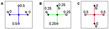
We now discuss the sensitivity of LLE’s weight vectors to noise. Figure 4 shows that an arbitrarily small change in the neighborhood can cause a large change in the weight vectors. This result can be understood by noting how the vector is obtained. It can be shown (Saul and Roweis, 2003) that equals , up to normalization. Sensitivity to noise is therefore expected when the condition number of is large (see Golub and Loan, 1983, Section 2). One way to solve this problem is to enforce regularization, with its associated problems (see section 2). In the next section we suggest a simple alternative solution to the sensitivity of LLE to noise.
One more implication of the fact that LLE preserves the high-dimensional neighborhood structure is that LLE’s output tends to a linear projection of the input data. Wu and Hu (2006) proved for a finite data set that when the reconstruction errors are exactly zero for each of the neighborhoods, and under some dimensionality constraint, the output of LLE must be a linear projection of the input data. Here, we present a simple argument that explains why LLE’s output tends to a linear projection when the number of input points tends to infinity, and show numerical examples that strengthen this claim. For simplicity, we assume that the input data is normalized.
Our argument is based on two claims. First, note that LLE’s output for dimension is a linear-projection of LLE’s output for dimension (see Section 2). Second, note that by definition, the LLE output is a set of points that minimizes the sum of reconstruction errors . For normalized input of dimension , when the number of input points tends to infinity, each point is well reconstructed by its neighboring points. Therefore the reconstruction error tends to zero for each point . This means that the input data tends to minimize the sum of reconstruction errors . Hence, the output points of LLE for output of dimension tend to the input points (up to a rotation). The result of these two claims is that any requested solution of dimension tends to a linear projection of the -dimensional solution, i.e., a linear projection of the input data.
The result that LLE tends to a linear projection is of asymptotical nature. However, numerical examples show that this phenomenon can occur even when the number of points is relatively small. This is indeed the case for the outputs of LLE shown in Figs. 1C, 2C, and 3C, for the open ring, the ‘S’ curve, and the swissroll, respectively.
4 Low-dimensional neighborhood representation for LLE
In this section we suggest a simple modification of LLE that computes the low-dimensional structure of the input points’ neighborhoods. Our approach is based on finding the best representation of rank (in the sense) for the neighborhood of each point, and then computing the weights with respect to these -dimensional neighborhoods. In Sections 5 and 6 we show theoretical results and numerical examples that justify our suggested modification.
We begin by finding a rank- representation for each local neighborhood. Recall that is the neighborhood matrix of , whose -th row is , where is the -th neighbor of . We assume that the number of neighbors is greater than , since otherwise cannot (in general) be reconstructed by its neighbors. We say that is the best rank- representation of , if minimizes over all the matrices of rank . Let be the SVD of , where and are orthogonal matrices of size and , respectively, and is a matrix, where are the singular values of for , ordered from the largest to the lowest, and for . We denote
| (4) |
where and are the first columns of and , respectively, and are the last and columns of and respectively, and and are of dimension and , respectively. Then by Corollary 2.3-3 of Golub and Loan (1983), can be written as .
We now compute the weight vectors for the -dimensional neighborhood . By (1), we need to find that minimize (see Section 2). The solution for this minimization problem is not unique, since by the construction all the vectors spanned by zero this function. Thus, our candidate for the weight vector is the vector in the span of that has the smallest norm. In other words, we are looking for
| (5) |
Note that we implicitly assume that . This is true whenever the neighborhood points are in general position, i.e., no of them lie in a -dimensional plane. To understand this, note that if then is of rank . Since is the projected neighborhood after centering, we obtained that the dimension of the centered projected neighborhood is of dimension , and not as assumed, and therefore the points are not in general position. See also Assumption (A2) in Section 5 and the discussion that follows.
The following Lemma shows how to compute the vector that minimizes (5).
Lemma 4.1.
Assume that the points of are in general position. Then the vector that minimizes (5) is given by
| (6) |
The proof is based on Lagrange multipliers and appears in Appendix A.1.
Following Lemma 4.1, we propose a simple modification for LLE based on computing the reconstruction vectors using -dimensional neighborhood representation.
Algorithm: LLE with low-dimensional neighborhood representation
Input: , an matrix.
Output: , an matrix.
Procedure:
1.
For each point find -nearest-neighbors and compute the neighborhood matrix .
2.
For each point compute the weight vector using the -dimensional neighborhood
representation:
•
Use the SVD decomposition to write .
•
Write .
•
Compute
3.
Compute the -dimension embedding by minimizing
(see (2)).
Note that the difference between this algorithm and LLE is in step (2). We compute the low-dimensional neighborhood representation of each neighborhood and obtain its weight vector, while LLE computes the weight vector for the original high-dimensional neighborhoods. One consequence of this approach is that the weight vectors are less sensitive to perturbation, as shown in Theorem 5.1. Another consequence is that the -dimensional output is no longer a projection of the embedding in dimension . This is because the weight vectors are computed differently for different values of output dimension . In particular, the input data no longer minimize , and therefore the linear projection problem does not occur.
From a computational point of view, the cost of this modification is small. For each point , the cost of computing the SVD of the matrix is . For neighborhoods we have which is of the same scale as LLE for this step. Since the overall computation of LLE is , the overhead of the modification has little influence on the running time of the algorithm (see Saul and Roweis, 2003, Section 4).
5 Theoretical results
In this section we prove two theoretical results regarding the computation of LLE using the low-dimensional neighborhood representation. We first show that a small perturbation of the neighborhood has a small effect on the weight vector. Then we show that the set of original points in the low-dimensional domain that are the pre-image of the input points achieve a low value of the objective function .
We start with some definitions. Let be a compact set and let be a smooth conformal mapping. This means that the inner products on the tangent bundle at each point are preserved up to a scalar that may change continuously from point to point. Note that the class of isometric embeddings is included in the class of conformal embeddings. Let be the -dimensional image of in . Assume that the input is a sample taken from . For each point , define the neighborhood and its low-dimensional representation as in Section 4. Let and be the SVDs of the -th neighborhood and its projection, respectively. Denote the singular values of by , where if . Denote the mean vector of the projected -th neighborhood by .
For the proofs of the theorems we require that the local high-dimensional neighborhoods satisfy the following two assumptions.
- (A1)
For each , .
More specifically, it is enough to demand . - (A2)
There is an such that for all , .
The first assumption states that for each , the neighborhood is essentially -dimensional. The second assumption was shown to be equivalent to the requirement that points in each projected neighborhood are in general position (see discussion in Section 3). We now show that this is equivalent to the requirement that the variance-covariance matrix of the projected neighborhood is not degenerate. Denote , then
Note that since is positive definite, so is . Since the only eigenvalues of are and , we obtain that .
Theorem 5.1.
See proof in Appendix A.3. Note that the assumption that can always be fulfilled by rescaling the matrix since rescaling the input matrix has no influence on the value of .
Fig 4 demonstrates why no bound similar to Theorem 5.1 exists for the weights computed by LLE. In the example we see a point on the grid with its -nearest neighbors, where some noise was added. While , and is arbitrary, the distance between each pair of vectors is at least . The bound of Theorem 5.1 states that for and the upper bounds on the distance when using the low-dimensional neighborhood representation are is and respectively. The empirical results shown in Fig 5 are even lower.

For the second theoretical result we require some additional definitions.
The minimum radius of curvature is defined as follows:
where varies over all unit-speed geodesics in and is in a domain of .
The minimum branch separation is defined as the largest positive number for which implies , where and is the geodesic distance between and (see Bernstein et al., 2000, for both definitions).
Define the radius of neighborhood to be
where is the -th neighbor of . Finally, define to be the maximum over .
We say that the sample is dense with respect to the chosen neighborhoods if . Note that this condition depends on the manifold structure, the given sample, and the choice of neighborhoods. However, for a given compact manifold, if the distribution that produces the sample is supported throughout the entire manifold, then this condition is valid with probability increasing towards as the size of the sample is increased and the radius of the neighborhoods is decreased.
Theorem 5.2.
See proof in Appendix A.3.
The theorem states that the original pre-image data has a small value of and thus is a reasonable embedding, although not necessarily the minimizer (Goldberg et al., 2008, see). This observation is not trivial from two reasons. First, it is not known a-priori that , the pre-image of the neighbors of , are also neighbors of . When short-circuits occur, this need not to be true (Balasubramanian et al., 2002, see). Second, the weight vectors characterized the projected neighborhood, which is only an approximation to the true neighborhood. Nevertheless, the theorem shows the has a low value.
6 Numerical results
In this section we present empirical results for LLE and LLE with low-dimensional neighborhood representation on some data sets. For LLE, we used the Matlab code as appears in LLE website (Saul and Roweis, ). The code for LLE with low-dimensional neighborhood representation is based on the LLE code and differs only in step (2) of the algorithm and is available in JRhomepage..
We ran LLE with low-dimensional neighborhood representation on the data sets of the open ring, the ‘S’-curve and the swissroll that appear in Figs 1-3. We used the same parameters for both LLE and LLE with low-dimensional neighborhood representation ( for the open ring and for the ‘S’-curve and the swissroll). The results appear in Fig 6.

We ran both LLE and LLE with low-dimensional neighborhood representation on by pixel images of a face, rendered with different poses and lighting directions. The images and their respective poses and lighting directions can be found at the Isomap webpage (Tenenbaum et al., ). The results of LLE, with , are given in Fig. 7. We also checked for ; in all cases LLE does not succeed in retrieving the pose and lighting directions. The results for LLE with low-dimensional neighborhood representation, also with , appear in Fig 8. The left-right pose and the lighting directions were discovered by LLE with low-dimensional neighborhood representation. We also checked for ; the results are roughly the same.


acknowledgments-disclosure-of-funding.
This research was supported in part by Israeli Science Foundation grant. Helpful discussions with Alon Zakai and Jacob Goldberger are gratefully acknowledged.Appendix A Proofs
A.1 Proof of Lemma 4.1
Proof.
Write . The Lagrangian of the problem can be written as
Taking derivatives with respect to both and , we obtain
Hence we obtain that . ∎
A.2 Proof of Theorem 5.1
Proof.
The proof of Theorem 5.1 consists of two steps. First, we find a representation of the vector , the weight vector of the perturbed neighborhood, see (12). Then we bound the distance between and , the weight vector of the original neighborhood.
We start with some notations. For every matrix , let be the -th singular value of . Note that . In this notation, we have . Denote by and . Using the decomposition of (4), we may write and . Note that . Define and to be the matrices of the left-singular vectors corresponding to the lowest singular values, as in (4).
Note that by assumption, , hence, . By Corollary 8.1-3 of Golub and Loan (1983),
| (8) |
Let . By Theorem 8.1-7 of Golub and Loan (1983), there is a matrix such that and such that the columns of are an orthogonal basis for an invariant subspace of . We want to show that and spans the same subspaces. To prove this, we bound the largest singular value of , and the result follows from (8).
First, note that
| (9) |
Hence,
| (10) | |||||
We now obtain some bounds on the size of . By assumption we have . Since assumption (A1) holds, we may assume that . Recall that and that . Isolating we obtain that . Similarly, we can show that . We also have , since by assumption , and similarly, . Summarizing, we have
| (11) |
We are now ready to bound the expression in (10). We have that since ; by assumption; since ; since and also ; since and ; since and . Combining all these bounds, we obtain
Hence, by (8) we have . Since spans a subspace of dimension, it must span the subspace with the vectors with lowest singular values of . In other words, spans the same subspace as or equivalently . Summarizing, we obtained that
| (12) |
We are now ready to bound the difference between and .
We use Assumption (A2) to obtain a bound on . Denote the projection of the normalized vector on the basis by . We have that
By assumption (A2), . Hence . Since , we have that
| (13) |
Similarly, we obtain a bound on .
where we used . Since by assumption , and using the facts that and , we obtain that . Hence, .
Finally, we obtain a bound on .
where the last inequality follows from (9), the fact that for any eigenvector of with eigenvalue , is also eigenvector of with eigenvalue , and the fact that for every matrix with orthonormal columns (Golub and Loan, 1983, see). Consequently,
where we used .
Combining these results, we have
where we used .
∎
A.3 Proof of Theorem 5.2
Proof.
Since , we bound each summand separately in order to obtain a global bound.
Let the induced neighbors of be defined by . Note that a-priori, it is not clear that are neighbors of . Let be the Jacobian of the function at . Since is a conformal mapping, , for some positive . Using first order approximation we have that . Hence, for we have,
Thus we have
| (14) |
We bound for the vector that minimizes (5). Note that by (4), . However, by construction . Hence
where we used the facts that for a any matrix , and that for a matrix with orthonormal columns (see Section 2 of Golub and Loan, 1983, for both). Substituting in (14), we obtain
As is an conformal mapping, we have , where is the geodesic metric and is the minimum of the scale function that measures the scaling change of at . The minimum is attained as is compact. The last inequality holds true since the geodesic distance is equal to the integral over for some path between and .
The sample is assumed to be dense, hence , where is the minimum branch separation (see Section 5). Using Bernstein et al. (2000), Lemma 3, we conclude that
References
- Balasubramanian et al. (2002) M. Balasubramanian, E. L. Schwartz, J. B. Tenenbaum, V. de Silva, and J. C. Langford. The isomap algorithm and topological stability. Science, 295(5552):7, 2002.
- Belkin and Niyogi (2003) M. Belkin and P. Niyogi. Laplacian Eigenmaps for Dimensionality Reduction and Data Representation. Neural Comp., 15(6):1373–1396, 2003.
- Bernstein et al. (2000) M. Bernstein, V. de Silva, J. C. Langford, and J. B. Tenenbaum. Graph approximations to geodesics on embedded manifolds. Technical report, Stanford University, Stanford, Available at http://isomap.stanford.edu, 2000.
- Chang and Yeung (2006) H. Chang and D. Y. Yeung. Robust locally linear embedding. Pattern Recognition, 39(6):1053–1065, 2006.
- Chen et al. (2007) J. Chen, R. Wang, S. Yan, S. Shan, X. Chen, and W. Gao. Enhancing human face detection by resampling examples through manifolds. Systems, Man and Cybernetics, Part A, IEEE Transactions on, 37(6):1017–1028, 2007.
- Donoho and Grimes (2004) D.L. Donoho and C. Grimes. Hessian eigenmaps: Locally linear embedding techniques for high-dimensional data. Proc. Natl. Acad. Sci. U.S.A., 100(10):5591–5596, 2004.
- Goldberg et al. (2008) Y. Goldberg, A. Zakai, D. Kushnir, and Y. Ritov. Manifold learning: The price of normalization. To appear in JMLR, 2008.
- Golub and Loan (1983) G. H. Golub and C. F. Van Loan. Matrix Computations. Johns Hopkins University Press, Baltimore, Maryland, 1983.
- Hadid and Pietikäinen (2003) A. Hadid and M. Pietikäinen. Efficient locally linear embeddings of imperfect manifolds. pages 188–201. 2003.
- Lee and Verleysen (2007) J. A. Lee and M. Verleysen. Nonlinear Dimensionality Reduction. Springer, 2007.
- L’Heureux et al. (2004) P. J. L’Heureux, J. Carreau, Y. Bengio, O. Delalleau, and S. Y. Yue. Locally linear embedding for dimensionality reduction in qsar. J. Comput. Aided Mol. Des., 18:475–482, 2004.
- Roweis and Saul (2000) S. T. Roweis and L. K. Saul. Nonlinear dimensionality reduction by locally linear embedding. Science, 290(5500):2323–2326, 2000.
- (13) L. K. Saul and S. T. Roweis. Locally Linear Embedding (LLE) homepage. http://www.cs.toronto.edu/~roweis/lle/.
- Saul and Roweis (2003) L. K. Saul and S. T. Roweis. Think globally, fit locally: unsupervised learning of low dimensional manifolds. J. Mach. Learn. Res., 4:119–155, 2003. ISSN 1533-7928.
- Shi et al. (2005) R. Shi, I. F. Shen, and W. Chen. Image denoising through locally linear embedding. In CGIV ’05: Proceedings of the International Conference on Computer Graphics, Imaging and Visualization, pages 147–152. IEEE Computer Society, 2005.
- (16) J. B. Tenenbaum, V. de Silva, and J. C. Langford. Isomap homepage. http://isomap.stanford.edu/.
- Tenenbaum et al. (2000) J. B. Tenenbaum, V. de Silva, and J. C. Langford. A global geometric framework for nonlinear dimensionality reduction. Science, 290(5500):2319–2323, 2000.
- Varini et al. (2006) C. Varini, A. Degenhard, and T. W. Nattkemper. Isolle: Lle with geodesic distance. Neurocomputing, 69(13-15):1768–1771, 2006.
- Wang et al. (2006) H. Wang, J. Zheng, Z. Yao, and L. Li. Improved locally linear embedding through new distance computing. pages 1326–1333. 2006.
- Wang et al. (2005) M. Wang, H. Yang, Z. H. Xu, and K. C. Chou. Slle for predicting membrane protein types. J. Theor. Biol., 232(1):7–15, 2005.
- Weinberger and Saul (2006) K. Q. Weinberger and L. K. Saul. Unsupervised learning of image manifolds by semidefinite programming. International Journal of Computer Vision, 70(1):77–90, 2006.
- Wu and Hu (2006) F. C. Wu and Z. Y. Hu. The LLE and a linear mapping. Pattern Recognition, 39(9):1799–1804, 2006.
- Xu et al. (2008) W. Xu, X. Lifang, Y. Dan, and H. Zhiyan. Speech visualization based on locally linear embedding (lle) for the hearing impaired. In BMEI (2), pages 502–505, 2008.
- Xu et al. (2006) X. Xu, F. C. Wu, Z. Y. Hu, and A. L. Luo. A novel method for the determination of redshifts of normal galaxies by non-linear dimensionality reduction. Spectroscopy and Spectral Analysis, 26(1):182–186, 2006.
- Zhang and Wang (2007) Z. Zhang and J. Wang. Mlle: Modified locally linear embedding using multiple weights. In B. Schölkopf, J. Platt, and T. Hoffman, editors, Advances in Neural Information Processing Systems 19, pages 1593–1600. MIT Press, Cambridge, MA, 2007.
- Zhang and Zha (2004) Z. Y. Zhang and H. Y. Zha. Principal manifolds and nonlinear dimensionality reduction via tangent space alignment. SIAM J. Sci. Comp, 26(1):313–338, 2004.