From Kadanoff-Baym dynamics to off-shell parton transport
Abstract
The description of strongly interacting quantum fields is based on two-particle irreducible (2PI) approaches that allow for a consistent treatment of quantum systems out-of-equilibrium as well as in thermal equilibrium. As a theoretical test case the quantum time evolution of -field theory in 2+1 space-time dimensions is investigated numerically for out-of-equilibrium initial conditions on the basis of the Kadanoff-Baym-equations including the tadpole and sunset self energies. In particular we address the dynamics of the spectral (‘off-shell’) distributions of the excited quantum modes and the different phases in the approach to equilibrium described by Kubo-Martin-Schwinger relations for thermal equilibrium states. A detailed comparison of the full quantum dynamics to approximate schemes like that of a standard kinetic (on-shell) Boltzmann equation is performed. We find that far off-shell processes are responsible for chemical equilibration, which is not included in the Boltzmann limit. Furthermore, we derive generalized transport equations for the same theory in a first order gradient expansion in phase space thus explicitly retaining the off-shell dynamics as inherent in the time-dependent spectral functions. The solutions of these equations compare very well with the exact solutions of the full Kadanoff-Baym equations with respect to the occupation numbers of the individual modes, the spectral evolution as well as the chemical equilibration process. Furthermore, the proper equilibrium off-shell distribution is reached for large times contrary to the quasiparticle Boltzmann limit. We additionally present a direct comparison of the solution of the generalized transport equations in the Kadanoff-Baym (KB) and Botermans-Malfliet (BM) form; both solutions are found to agree very well with each other. The off-shell transport equation in the BM scheme allows for an explicit solution within an extended dynamical quasiparticle Ansatz. This leads to generalized equations of motion for dynamical quasiparticles that exceed the classical Hamilton equations and allow for the description of dynamical spectral functions. The dynamical quasiparticle model (DQPM) is used to extract partonic spectral functions from lattice QCD in the temperature range 0.8 10. By consideration of time-like and space-like sectors of ’observables’ such as number densities, energy densities etc. mean-field potentials as well as effective interactions are extracted at different temperature and quark chemical potentials . The latter determine the off-shell dynamics in the Parton-Hadron-String Dynamics (PHSD) transport approach. Illustrative examples for off-shell dynamics in the hadron and parton sector are presented for production from nucleus-nucleus collisions from SIS to RHIC energies. The generalized transport approach, furthermore, qualifies for the description of hadronization without leading to the problem of entropy reduction as in conventional coalescence models.
Introduction
Non-equilibrium many-body theory or quantum field theory has become a major topic of research for transport processes in nuclear physics, in cosmological particle physics as well as condensed matter physics. The multidisciplinary aspect arises due to a common interest to understand the various relaxation phenomena of quantum dissipative systems. Recent progress in cosmological observations has also intensified the research on quantum fields out of equilibrium. Important questions in high-energy nuclear or particle phyics at the highest energy densities are: i) how do nonequilibrium systems in extreme environments evolve, ii) how do they eventually thermalize, iii) how phase transitions do occur in real time with possibly nonequilibrium remnants, and iv) how do such systems evolve for unprecedented short and nonadiabatic timescales?
The very early history of the universe provides important scenarios, where non-equilibrium effects might have played an important role, like in the (post-) inflationary epoque (see e.g. [1, 2, 3, 4]), for the understanding of baryogenesis (see e.g. [1, 5]) and also for the general phenomena of cosmological decoherence [6]. Referring to modern nuclear physics the dynammics of heavy-ion collisions at various bombarding energies has always been a major motivation for research on nonequilbrium quantum many-body physics and relativistic quantum-field theories, since the initial state of a collision resembles an extreme nonequilibrium situation while the final state might even exhibit a certain degree of thermalization. Indeed, at the presently highest energy heavy-ion collider experiments at RHIC, where one expects to create experimentally a transient deconfined state of matter denoted as quark-gluon plasma (QGP) [7], there are experimental indications - like the build up of collective flow - for an early thermalization accompanied with the build up of a very large pressure. These examples demonstrate that one needs an ab-initio understanding of the dynamics of out-of-equilibrium quantum-field theory.
Especially the powerful method of the ‘Schwinger-Keldysh’ [8, 9, 10, 11, 12] or ‘closed time path’ (CTP) (non-equilibrium) real-time Greens functions has been shown to provide an appropriate basis for the formulation of the complex problems in the various areas of nonequilibrium quantum many-body physics. Within this framework one can derive valid approximations - depending, of course, on the problem under consideration - by preserving overall consistency relations. Originally, the resulting causal Dyson-Schwinger equation of motion for the one-particle Greens functions (or two-point functions), i.e. the Kadanoff-Baym (KB) equations [13], have served as the underlying scheme for deriving various transport phenomena and generalized transport equations. For review articles on the Kadanoff-Baym equations in the various areas of nonequilibrium quantum physics we refer the reader to Refs. [14, 15, 16, 17, 18, 19]. We note in passing, that also the ’influence functional formalism’ has been shown to be directly related to the KB equations [20]. Such a relation allows to address inherent stochastic aspects of the latter and also to provide a rather intuitive interpretation of the various self-energy parts that enter the KB equations.
Furthermore, kinetic transport theory is a convenient tool to study many-body nonequilibrium systems, nonrelativistic or relativistic. Kinetic equations, which do play the central role in more or less all practical simulations, can be derived by means of appropriate KB equations within suitable approximations. Hence, a major impetus in the past has been to derive semi-classical Boltzmann-like transport equations within the standard quasi-particle approximation. Additionally, off-shell extensions by means of a gradient expansion in the space-time inhomogenities - as already introduced by Kadanoff and Baym [13] - have been formulated: for an relativistic electron-photon plasma [21], for transport of electrons in a metal with external electrical field [22, 23], for transport of nucleons at intermediate heavy-ion reactions [24], for transport of particles in -theory [18, 25], for transport of electrons in semiconductors [19, 26], for transport of partons or fields in high-energy heavy-ion reactions [30, 31, 32, 33], or for a trapped Bose system described by effective Hartree-Fock-Bogolyubov kinetic equations [34]. We recall that on the formal level of the KB-equations the various forms assumed for the self-energy have to fulfill consistency relations in order to preserve symmetries of the fundamental Lagrangian [13, 35, 36]. This allows also for a unified treatment of stable and unstable (resonance) particles.
In non-equilibrium quantum-field theory typically the nonperturbative description of (second-order) phase transitions has been in the foreground of interest by means of mean-field (Hartree) descriptions [2, 8, 37, 38, 39], with applications for the evolution of disoriented chiral condensates or the decay of the (oscillating) inflaton in the early reheating era of the universe. ‘Effective’ mean-field dissipation (and decoherence) - solving the so called ‘backreaction’ problem - was incorporated by particle production through order parameters explicitly varying in time. However, it had been then realized that such a dissipation mechanism, i.e. transferring collective energy from the time-dependent order parameter to particle degrees of freedom, can not lead to true dissipation and thermalization. Such a conclusion has already been known for quite some time within the effective description of heavy-ion collisions at low energy. Full time-dependent Hartree or Hartree-Fock descriptions [40] were insufficient to describe the reactions with increasing collision energy; additional Boltzmann-like collision terms had to be incorporated in order to provide a more adequate description of the collision processes.
The incorporation of true collisions then has been formulated also for various quantum-field theories [41, 42, 43, 44, 45, 46]. Here, a systematic expansion of the ”2PI effective action” is conventionally invoked [18, 37, 46] serving as a nonperturbative expansion parameter. Of course, only for large this might be a controlled expansion. In any case, the understanding and the influence of dissipation with the chance for true thermalization - by incorporating collisions - has become a major focus of recent investigations. The resulting equations of motion always do resemble the KB equations; in their general form (beyond the mean field or Hartree(-Fock) approximation) they do break time invariance and thus lead to irreversibility. This macroscopic irreversibility arises from the truncations of the full theory to obtain the self-energy operators in a specific limit. As an example we mention the truncation of the (exact) Martin-Schwinger hierarchy in the derivation of the collisional operator in Ref. [24] or the truncation of the (exact) BBGKY hierarchy in terms of -point functions [24, 41, 42, 47].
In principle, the non-equilibrium quantum dynamics is nonperturbative in nature. Unphysical singularities only appear in a limited truncation scheme, e.g. ill-defined pinch singularities [48], which do arise at higher order in a perturbative expansion in out of equilibrium quantum-field theory, are regularized by a consistent nonperturbative description (of Schwinger-Dyson type) of the non-equilibrium evolution, since the resummed propagators obtain a finite width [49]. Such a regularization is also observed by other resummation schemes like the dynamical renormalization-group technique [45, 50].
Although the analogy of KB-type equations to a Boltzmann-like process is quite obvious, this analogy is far from being trivial. The full quantum formulation contains much more information than a semi-classical (generally) on-shell Boltzmann equation. The dynamics of the spectral (i.e. ‘off-shell’) information is fully incorporated in the quantum dynamics while it is missing in the Bolzmann limit. A full answer to the question of quantum equilibration can thus only be obtained by detailed numerical solutions of the quantum description itself.
We briefly address previous works that have investigated numerically approximate or full solutions of KB-type equations. A seminal work has been carried out by Danielewicz [51], who investigated for the first time the full KB equations for a spatially homogenous system with a deformed Fermi sphere in momentum space for the initial distribution of occupied momentum states in order to model the initial condition of a heavy-ion collision in the nonrelativistic domain. In comparison to a standard on-shell semi-classical Boltzmann equation the full quantum Boltzmann equation showed quantitative differences, i.e. a larger collective relaxation time for complete equilibration of the momentum distribution . This slowing down of the quantum dynamics was attributed to quantum interference and off-shell effects. Similar quantum modifications in the equilibration and momentum relaxation have been found for a relativistic situation in Ref. [52]. In the following, full and more detailed solutions of nonrelativistic KB equations have been performed by Köhler [53, 54] with special emphasis on the build up of initial many-body correlations on short time scales. The role of memory effects has been clearly shown experimentally by femtosecond laser spectroscopy in semiconductors [55] in the relaxation of excitons. Solutions of quantum transport equations for semiconductors [19, 56] - to explore relaxation phenomena on short time and distance scales - has become also a very active field of research [22, 57].
In the last decade the numerical treatment of general out-of-equilibrium quantum dynamics, as described within 2PI effective approaches at higher order, have become more frequent. The subsequent equations of motion are very similar to the KB equations, although more involved expressions for a non-local vertex function - as obtained by the 2PI scheme - are incorporated. The numerical solutions are also obtained only for homogenous systems, so far (cf. [58, 59, 60, 61, 62, 63]).
Apart from complete thermalization of all single-particle degrees of freedom the quantum dynamics of the spectral function is also a lively discussed issue in the microscopic modeling of hadronic resonances with a broad mass distribution. This is of particular relevance for simulations of heavy-ion reactions, where e.g. the -resonance or the -meson already show a large decay witdh in vacuum [64, 65, 66, 67, 68, 69]. Especially the vector meson represents the most promising hadronic particle for showing possible in-medium modifications in hot and compressed nuclear matter since the leptonic decay products are of only weakly interacting electromagnetic nature. Hence a consistent formulation for the transport of extremely short-lived particles beyond the standard quasi-particle approximation is needed. On the one side, there exist purely formal developments starting from a first-order gradient expansion of the underlying KB equations [67, 68, 69], while on the other side already practical realisations for various questions have emerged [64, 65, 66, 70]. The general idea is to obtain a description for the propagation of dynamical spectral functions, i.e. a propagation in the off-shell mass squared .
The aim of these lectures is to provide a short survey on (nonperturbative) nonequilibrium quantum field theory with actual applications (and numerical illustrations) for the model case of scalar -theory. This includes the derivation of off-shell as well as on-shell (Boltzmann) transport equations and their comparison to the exact solution for a variety of out-of-equilibrium initial conditions. Furthermore, a generalized testparticle Ansatz is introduced that allows for a convenient solution of off-shell transport equations which involve only the complex (retarded) selfenergies for the relevant degrees of freedom. In case of hadrons these selfenergies may be determined from effective Lagrangian models whereas in case of partons suitable selfenergies can be fixed by the dynamical quasiparticle model in comparison to lattice QCD at finite temperature . Applications for dilepton production in nucleus-nucleus collisions provide a practical case for the spectral off-shell dynamics and bridge the gap to current spectra taken by various experimenal collaborations [71]. On the partonic side we present an illustrative example for the build up of collective flow, strangeness equilibration as well as the dynamics of hadronization.
1 Quantum field dynamics and thermalization
1.1 Non-equilibrium dynamics
1.1.1 The Kadanoff-Baym equations
As mentioned in the Introduction, a natural starting point for non-equilibrium theory is provided by the closed-time-path (CTP) method. Here all quantities are given on a special real-time contour with the time argument running from to on the chronological branch and returning from to on the antichronological branch . In cases of systems prepared at a time this value is (instead of ) the start and end point of the real-time contour (cf. Fig. 1). In particular the path ordered Green functions (in case of real scalar fields ) are defined as
| (1) | |||||
where the operator orders the field operators according to the position of their arguments on the real-time path as accomplished by the path step-functions . The expectation value in (1) is taken with respect to some given density matrix , which is constant in time, while the operators in the Heisenberg picture contain the entire time dependence of the non-equilibrium system, i.e. .

Self-consistent equations of motion for these Green functions can be obtained with help of the two-particle irreducible (2PI) effective action . It is given by the Legendre transform of the generating functional of the connected Green functions as
| (2) |
in case of vanishing vacuum expectation value . In (2) depends only on free Green functions and is treated as a constant, while the symbols represent convolution integrals over the closed time path in Fig. 1. The functional is the sum of all closed diagrams built up by full propagators ; it determines the self-energies by functional variation as
| (3) |
From the effective action the equations of motion for the Green function are determined by the stationarity condition
| (4) |
1.1.2 -theory
The scalar -theory is an example for a fully relativistic field theory of interacting scalar particles that allows to test theoretical approximations [41, 42] without coming to the problems of gauge-invariant truncation schemes as encountered for gauge (vector) fields [41, 58, 59, 60]. Its Lagrangian density is given by
| (5) |
where denotes the ’bare’ mass and is the coupling constant determining the interaction strength of the scalar fields.
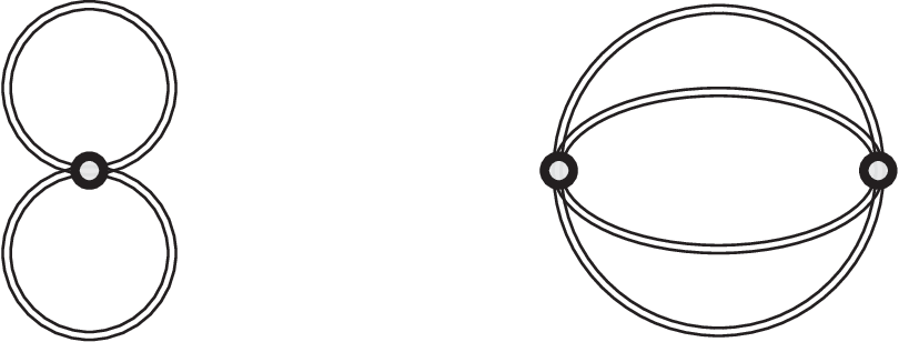
In the present calculation we take into account contributions up to the 3-loop order for the -functional (cf. Fig. 2) which reads explicitly
| (6) |
where denotes the spatial dimension of the problem.
This approximation corresponds to a weak coupling expansion such that we consider contributions up to the second superficial order in the coupling constant (cf. Fig. 3). For the superficial coupling constant order we count the explicit coupling factors associated with the visible vertices. The hidden dependence on the coupling strength - which is implicitly incorporated in the self-consistent Green-functions that built up the -functional and the self-energies - is ignored on that level. For our present purpose this approximation is sufficient since we include the leading mean-field effects as well as the leading order scattering processes that pave the way to thermalization.
For the actual calculation it is advantageous to change to a single-time representation for the Green functions and self-energies defined on the closed-time-path. In line with the position of the coordinates on the contour there exist four different two-point functions
| (7) | |||||
Here represent the (anti-)time-ordering operators in case of both arguments lying on the (anti-)chronological branch of the real-time contour. These four functions are not independent of each other. In particular the non-continuous functions and are built up by the Wightman functions and and the usual -functions in the time coordinates. Since for the real boson theory (5) the relation holds, the knowledge of the Green functions for all characterizes the system completely. Nevertheless, we will give the equations for and explicitly since this is the familiar representation for general field theories [25].
By using the stationarity condition for the action (4) and resolving the time structure of the path ordered quantities we obtain the Kadanoff-Baym equations for the time evolution of the Wightman functions [58, 72]:
| (8) | |||||
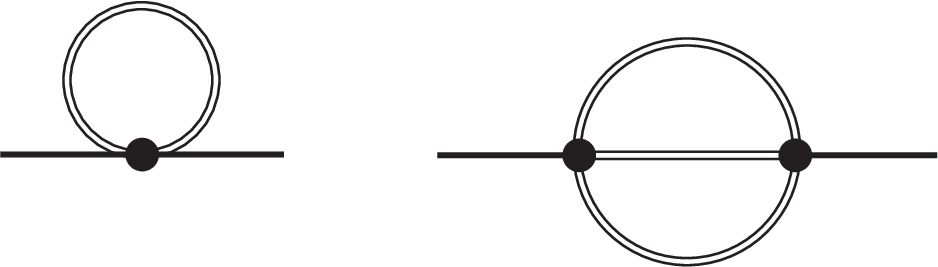
Within the 3-loop approximation for the 2PI effective action (i.e. the -functional (6)) we get two different self-energies: In leading order of the coupling constant only the tadpole diagram (l.h.s. of Fig. 3) contributes and leads to the generation of an effective mass for the field quanta. This self-energy (in coordinate space) is given by
| (9) |
and is local in space and time. In next order in the coupling constant (i.e. ) the non-local sunset self-energy (r.h.s. of Fig. 3) enters the time evolution as
| (10) | |||
| (11) |
Thus the Kadanoff-Baym equation (8) in our case includes the influence of a mean-field on the particle propagation – generated by the tadpole diagram – as well as scattering processes as inherent in the sunset diagram.
The Kadanoff-Baym equation describes the full quantum nonequilibrium time evolution on the two-point level for a system prepared at an initial time , i.e. when higher order correlations are discarded. The causal structure of this initial value problem is obvious since the time integrations are performed over the past up to the actual time (or , respectively) and do not extend to the future.
Furthermore, also linear combinations of the Green functions in single-time representation are of interest and will be exploited for the spectral properties of the system later on. The retarded Green function and the advanced Green function are given as
| (12) | |||||
| (13) | |||||
These Green functions contain exclusively spectral, but no statistical information of the system. Their time evolution is determined by Dyson-Schwinger equations and given by (cf. Ref. [72])
| (14) | |||
| (15) | |||
where the retarded and advanced self-energies , are defined via , similar to the Green functions. Thus the retarded (advanced) Green functions are determined by retarded (advanced) quantities, only.
1.1.3 Homogeneous systems in space
In the following we will consider homogeneous systems in space. To obtain a numerical solution the Kadanoff-Baym equation (8) is transformed to momentum space:
| (16) | |||||
where both memory integrals are summarized in the function . The equation of motion in the second time direction is given analogously. In two-time and momentum space () representation the self-energies read
| (17) | |||||
1.2 Numerical studies on equilibration
1.2.1 Numerical implementation
For the solution of the Kadanoff-Baym equations (16) a flexible and accurate algorithm has been developed: Instead of solving the second order differential equation (16) one can generate a set of first order differential equations for the Green functions in the Heisenberg picture,
| (18) | |||||
with the canonical field momentum . The first index or is always related to the first space-time argument. Exploiting the time-reflection symmetry of the Green functions some of the differential equations are redundant. The required equations of motion are given as
| (19) | |||||
where is the mean time variable. Thus one explicitly considers the propagation in the time diagonal (cf. Ref. [53]). In the equations of motion (19) the current (renormalized) effective energy including the time dependent tadpole contribution enters,
| (20) |
with and specified in the next Subsection. The evolution in the direction has not be taken into account for and since the Green functions beyond the time diagonal () are determined via the time reflection symmetry from the known values for the lower time triangle in both cases. Since there is no time reflection symmetry for the functions, they have to be calculated (and stored) in the whole , range. However, we can ignore the evolution of since it is obtained by the relation . The correlation integrals in (19) are given by
| (21) | |||||
| (22) | |||||
In (19) and (22) one can replace such that the set of equations is closed in the Green functions , and .
The disadvantage, to integrate more Green functions in time in this first-order scheme, is compensated by its good accuracy. As mentioned before, we especially take into account the propagation along the time diagonal which leads to an improved numerical precision. The set of differential equations (19) is solved by means of a 4th order Runge-Kutta algorithm. For the calculation of the self energies a Fourier method similar to Refs. [15, 53] is applied. The self energies (17), furthermore, are calculated in coordinate space where they are products of coordinate-space Green functions (that are available by Fourier transformation) and finally transformed to momentum space.
1.2.2 Renormalization of -theory in 2+1 dimensions
In 2+1 space-time dimensions both self-energies (9), (10) incorporated in the present case are ultraviolet divergent. Since the particles have a finite mass no problems arise from the infrared momentum regime. The ultraviolet regime, however, has to be treated explicitly.
For the renormalization of the divergences we only assume that the time-dependent nonequilibrium distribution functions are decreasing for large momenta comparable to the equilibrium distribution functions, i.e exponentially. Thus one can apply the conventional finite temperature renormalization scheme. By separating the real time (equilibrium) Green functions into vacuum () and thermal parts it becomes apparent, that only the pure vacuum contributions of the self-energies are divergent. For the linear divergent tadpole diagram a mass counter term (at the renormalized mass ) can be introduced as
| (23) |
which cancels the contribution from the momentum integration of the vacuum part of the Green function.
In case of the sunset diagram only the logarithmically divergent pure vacuum part requires a renormalization, while it remains finite as long as at least one temperature line is involved. Contrary to the case of 3+1 dimensions it is not necessary to employ the involved techniques developed for the renormalization of self-consistent theories (in equilibrium) in Refs. [73] because in 2+1 dimensions theory is superrenormalizable. Since the divergence only appears (in energy-momentum space) in the real part of the Feynman self-energy at (and equivalently in the real part of the retarded/advanced self-energies ), it can be absorbed by another mass counterterm
| (24) | |||||
at given four-momentum and renormalized mass .
.
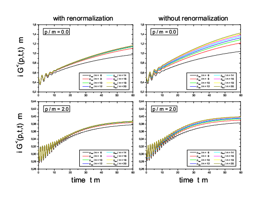
In Fig. 4 we demonstrate the applicability of the renormalization prescription. To this aim we display two momentum modes (upper plots) and = 2.0 (lower plots) of the equal-time Green function for various momentum cut-offs with (left plots) and without (right plots) renormalization of the sunset self-energy. For both cases the renormalization of the tadpole diagram has been used. We mention, that a non-renormalization of the tadpole self-energy has even more drastic consequences in accordance with the linear degree of divergence. For the non-renormalized calculations – with respect to the sunset diagram – we observe that both momentum modes do not converge with increasing momentum space cut-off. In fact, all lines tend to infinity when the maximum momentum is enlarged (since the gridsize of the momentum grid is kept constant). Although the divergence as a function of the momentum cut-off is rather weak - in accordance with the logarithmic divergence of the sunset self-energy in 2+1 space-time dimensions - a proper ultraviolet limit is not obtained.
This problem is cured by the sunset mass counter term (24) as seen on the left side of Figure 4. For the momentum mode the calculations converge to a limiting curve with increasing momentum cut-off. Even for the more selective case of the mode of the equal-time Green function the convergence is established. We point out that this limit is obtained for the unequal-time Green functions as well (not shown here explicitly). In fact, it turns out that the equal-time functions provide the most crucial test for the applicability of the renormalization prescription, since the divergent behaviour appears to be less pronounced for the propagation along a single time direction or . Thus we can conclude that the renormalization scheme introduced above, i.e. including mass counter terms for the divergent tadpole and sunset self-energies, leads to ultraviolet stable results.
In the following Subsections we will use the ’bare’ mass = 1, which implies that times are given in units of the inverse mass or is dimensionless. Accordingly, the bare coupling in (7) is given in units of the mass such that is dimensionless, too.
1.2.3 Initial conditions
In order to investigate equilibration phenomena on the basis of the Kadanoff-Baym equations for the 2+1 dimensional problem, one first has to specify the initial conditions for the time integration. To this aim we consider four different initial distributions that are all characterized by the same energy density. Consequently, for large times () all initial value problems should lead to the same equilibrium final state. The initial equal-time Green functions adopted are displayed in Fig. 5 (l.h.s.) as a function of the momentum . We first concentrate on polar symmetric configurations due to the large numerical expense for this first investigation11 1 In Section 1.4 we will present also calculations for non-symmetric systems.. Since the equal-time Green functions are purely imaginary we show only the real part of in Fig. 5.
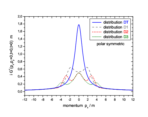
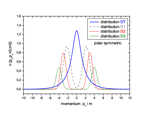
Furthermore, the corresponding initial distribution functions in the occupation density , related to via
| (25) |
are shown in Fig. 5 on the r.h.s. While the initial distributions D1, D2, D3 have the shape of (polar symmetric) ’tsunami’ waves with maxima at different momenta in , the initial distribution DT corresponds to a free Bose gas at a given initial temperature that is fixed by the initial energy density. According to (25) the difference between the Green functions and the distribution functions is basically given by the vacuum contribution, which has its maximum at small momenta. Thus even for the distributions D1, D2, D3 the corresponding Green functions are non-vanishing for 0.
Since we consider a finite volume we work in a basis of momentum modes characterized by the number of nodes in each direction. The number of momentum modes is typically in the order of 40 which is found to be sufficient for numerically stable results. For times we consider the systems to be noninteracting and switch on the interaction () for =0 to explore the quantum dynamics of the interacting system for .
1.2.4 Equilibration in momentum space
The time evolution of various (selected) momentum modes of the equal-time Green function for the different initial states D1, D2, D3 and DT is shown in Fig. 6, where the dimensionless time is displayed on a logarithmic scale. We observe that starting from very different initial conditions - as introduced above - the single momentum modes converge to the same respective occupation numbers for large times as characteristic for a system in equilibrium. As noted above, the initial energy density is the same for all distributions and energy conservation is fulfilled strictly in the time integration of the Kadanoff-Baym equations. The different momentum modes in Fig. 6 typically show a three-phase structure: For small times () one finds damped oscillations that can be identified with a typical switching-on effect at =0, where the system is excited by a sudden increase of the coupling constant to . The damping of the initial oscillations depends on the coupling strength and is more pronounced for strongly coupled systems. We mention that for very strong interactions the initial oscillations are even hard to recognize.
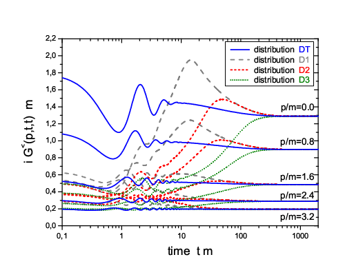
For ’intermediate’ time scales () one observes a strong change of all momentum modes in the direction of the final stationary state. We address this phase to ’kinetic’ equilibration and point out, that - depending on the initial conditions and the coupling strength - the momentum modes can temporarily even exceed their respective equilibrium value. This can be seen explicitly for the lowest momentum modes ( or ) of the distribution D1 in Fig. 6, which possesses initially maxima at small momentum. Especially the momentum mode of the equal-time Green function , which starts at around 0.52, is rising to a value of 1.95 before decreasing again to its equilibrium value of 1.29. Thus the time evolution towards the final equilibrium value is – after an initial phase with damped oscillations – not necessarily monotonic. For different initial conditions this behaviour may be weakened significantly as seen for example in case of the initial distribution D2 in Figure 6. Coincidently, both calculations D1 and D2 show approximately the same equal-time Green function values for times 80. Note, that for the initial distribution D3 the non-monotonic behaviour is not seen any more.
In general, one observes that only initial distributions (of the well type) show this feature during their time evolution, if the maximum is located at sufficiently small momenta. Initial configurations like the distribution DT - where the system at is given by a free gas of particles at a temperature - do not show this property. Although the DT distribution is not the equilibrium state of the interacting theory, the actual numbers are much closer to the equilibrium state of the interacting system than the initial distributions D1, D2 and D3. Therefore, the evolution for DT proceeds less violently. We point out, that in contrast to the calculations performed for -theory in 1+1 space-time dimensions [60] we find no power law behaviour for intermediate time scales.
The third phase, i.e. the late time evolution () is characterized by a smooth approach of the single momentum modes to their respective equilibrium values. As we will see in Section 1.4 this phase is adequately characterized by chemical equilibration processes.
1.3 The different phases of quantum equilibration
1.3.1 Build-up of initial correlations
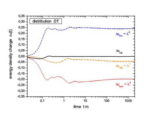
The time evolution of the interacting system within the Kadanoff-Baym equations is characterized by the build-up of early correlations. This can be seen from Fig. 7 where all contributions to the energy-density are displayed separately as a function of time and the total energy density is subtracted. The kinetic energy density is represented by all parts of that are independent of the coupling constant (). All terms proportional to are summarized by the tadpole energy density including the actual tadpole term as well as the corresponding tadpole mass counterterm (cf. Section 1.2.2). The contributions from the sunset diagram are represented by the sunset energy density .
| (26) | |||||
The calculation in Fig. 7 has been performed for the initial distribution DT (which represents a free gas of Bose particles at temperature ) with a coupling constant of . This state is stationary in the well-known Boltzmann limit (cf. Section 1.4), but it is not for the Kadanoff-Baym equation. In the full quantum calculations the system evolves from the uncorrelated initial state and the correlation energy density decreases rapidly with time. The decrease of the correlation energy which is – with exception of the sunset mass counterterm contribution – initially zero is approximately compensated by an increase of the kinetic energy density . Since the kinetic energy increases in the initial phase, the final temperature is slightly higher than the initial ’temperature’ . The remaining difference is compensated by the tadpole energy density such that the total energy density is conserved.
While the sunset energy density and the kinetic energy density always show a time evolution comparable to Fig. 7 the change of the tadpole energy density depends on the initial configuration and may be positive as well. Since the self energies are obtained within a -derivable scheme the fundamental conservation laws, as e.g. energy conservation, are respected to all orders in the coupling constant. When neglecting the sunset contributions and starting with a non-static initial state of identical energy density one observes the same compensating behaviour between the kinetic and the tadpole terms.
1.3.2 Time evolution of the spectral function
Within the Kadanoff-Baym calculations the full quantum information of the two-point functions is retained. Consequently, one has access to the spectral properties of the nonequilibrium system during its time evolution. The spectral function in our case is given by
| (27) |
From the dynamical calculations the spectral function in Wigner-space for each system time is obtained via Fourier transformation with respect to the relative time coordinate :
| (28) |
Note that a damping of the function in relative time corresponds to a finite width of the spectral function in Wigner-space. This width in turn can be interpreted as the inverse life time of the interacting scalar particle. We recall, that the spectral function – for all times and for all momenta – obeys the normalization
| (29) |
which is nothing but a reformulation of the equal-time commutation relation (or quantization) for the fields.
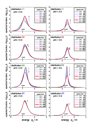
In Fig. 8 we display the time evolution of the spectral function for the initial distributions D1, D2 and DT for two different momentum modes and . Since the spectral functions are antisymmetric in energy for the momentum symmetric configurations considered, i.e. , we only show the positive energy part. For our initial value problem in two-times and space the Fourier transformation (28) is restricted for system times to an interval . Thus in the very early phase the spectral function assumes a finite width already due to the limited support of the Fourier transform in the interval and a Wigner representation is not very meaningful. We, therefore, present the spectral functions for various system times starting from up to .
For the free thermal initialization DT the evolution of the spectral function is very smooth and comparable to the smooth evolution of the equal-time Green function as discussed in Section 1.2.4. In this case the spectral function is already close to the equilibrium shape at small times being initially only slightly broader than for late times. The maximum of the spectral function (for all momenta) is higher than the (bare) on-shell value and nearly keeps its position during the whole time evolution. This results from a positive tadpole mass shift, which is only partly compensated by a downward shift originating from the sunset diagram.
The time evolution for the initial distributions D1, D2 and D3 has a richer structure. For the distribution D1 the spectral function is broad for small system times (see the line for ) and becomes a little sharper in the course of the time evolution (as presented for the momentum mode as well as for ). In line with the decrease in width the height of the spectral function is increasing (as demanded by the normalization property (29)). This is indicated by the small arrow close to the peak position. Furthermore, the maximum of the spectral function (which is approximately the on-shell energy) is shifted slightly upwards for the zero mode and downwards for the mode with higher momentum. Although the real part of the (retarded) sunset self-energy leads (in general) to a lowering of the effective mass, the on-shell energy of the momentum modes is still higher than the one for the initial mass (indicated by the ’on-shell’ arrow) due to the positive mass shift from the tadpole contribution.
For the initial distribution D3 we find the opposite behaviour. Here the spectral function is quite narrow for early times and increasing its width during the time evolution. Correspondingly, the height of the spectral function decreases with time. This behaviour is observed for the zero momentum mode as well as for the finite momentum mode . Especially in the latter case the width for early times is so small that the spectral function shows oscillations originating from the finite range of the Fourier-transformation from relative time to energy. Although we have already increased the system time for the first curve to (for the oscillations are much stronger) the spectral function is not fully resolved, i.e. it is not sufficiently damped in relative time in the interval available for the Fourier transform. For later times the oscillations vanish and the spectral function tends to the common equilibrium shape.
The time evolution of the spectral function for the initial distribution D2 is somehow in between the last two cases. Here the spectral function develops (at intermediate times) a slightly higher width than in the beginning before it is approaching the narrower static shape again. The corresponding evolution of the maximum is again indicated by the (bent) arrow. Finally, all spectral functions show the (same) equilibrium form represented by the solid gray line.
As already observed in Section 1.2.4 for the equal-time Green functions, we emphazise that there is no universal time evolution for the nonequilibrium systems. In fact, the evolution of the system during the equilibration process depends on the initial conditions. On the other hand, the time dependence of the spectral function is only moderate such that one might also work with some time-averaged or even the equilibrium spectral function. In order to investigate this issue in more quantitative detail we concentrate on the maxima and widths of the spectral functions in the following.
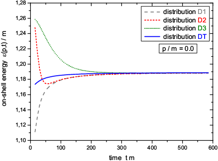
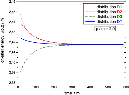
Since the solution of the Kadanoff-Baym equation provides the full spectral information for all system times the evolution of the on-shell energies can be studied as well as the spectral widths. In Fig. 9 we display the time dependence of the on-shell energies of the momentum modes (l.h.s.) and (r.h.s.) for the four initial distributions D1, D2, D3 and DT. We see that the on-shell energy for the zero momentum mode increases with time for the initial distribution D1 and to a certain extent for the free thermal distribution DT (as can be also extracted form Fig. 8). The on-shell energy of distribution D3 shows a monotonic decrease during the evolution while it passes through a minimum for distribution D2 before joining the line for the initialization D1. For momentum an opposite behaviour is observed. Here the on-shell energy for distribution D1 (and less pronounced for the distribution DT) are reduced in time whereas it is increased in the case of D3. The result for the initialization D2 is monotonous for this mode and matches the one for D1 already for moderate times. Thus we find, that the time evolution of the on-shell energies does not only depend on the initial conditions, but might also be different for various momentum modes. It turns out – for the initial distributions investigated – that the above described characteristics change around and are retained for larger momenta (not presented here).
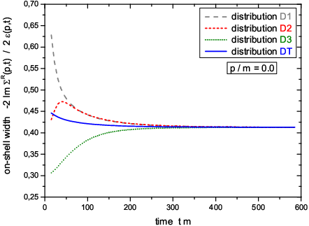
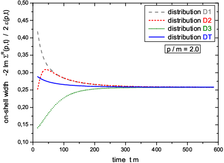
Furthermore, we present in Fig. 10 the time evolution of the on-shell width for the usual momentum modes for the different initial distributions. The on-shell width is given by the imaginary part of the retarded sunset self-energy at the on-shell energy of each respective momentum mode as
| (30) |
As already discussed in connection with Fig. 8 we observe for both momentum modes a strong decrease of the on-shell width for the initial distribution D1 associated with a narrowing of the spectral function. In contrast, the on-shell widths of distribution D3 increase with time such that the corresponding spectral functions broaden towards the common static shape. For the initialization D2 we observe an non-monotonic evolution of the on-shell widths connected with a broadening of the spectral function at intermediate times. Similar to the case of the on-shell energies we find, that the results for the on-shell widths of the distributions D1 and D2 coincide well above a certain system time. As expected from the lower plots of Fig. 8 the on-shell width for the free thermal distribution DT exhibits only a weak time dependence with a slight decrease in the initial phase of the time evolution.
In summarizing this Subsection we point out, that there is no universal time evolution of the spectral functions for the initial distributions considered. Peak positions and widths depend on the initial configuration and evolve differently in time. However, we find only effects in the order of 10% for the on-shell energies in the initial phase of the system evolution and initial variations of 50% for the widths of the dominant momentum modes. Thus, depending on the physics problem of interest, one might discard an explicit time-dependence of the spectral functions and adopt the equilibrium shape.
1.3.3 The equilibrium state
In Section 1.2 we have seen that arbitrary initial momentum configurations of the same energy density approach a stationary limit for , which is the same for all initial distributions. In this Subsection we will investigate whether this stationary state is the proper thermal state for interacting Bose particles.
As shown before, in the present calculations within the three-loop approximation of the 2PI effective action we describe kinetic equilibration via the sunset self-energies and also obtain a finite width for the particle spectral function, since the Green functions have a non-zero imaginary part (in energy space). It is not obvious, however, if the stationary state obtained for corresponds to the proper equilibrium state.
In order to clarify the nature of the asymptotic stationary state of our calculations we first change into Wigner space. The Green function and the spectral function in energy are obtained by Fourier-transformation with respect to the relative time at every system time ,
| (31) |
| (32) |
We recall, that the spectral function can also be obtained directly from the Green functions (cf. Section 1.1) by
| (33) |
Now we introduce the energy and momentum dependent distribution function at any system time by the definition
| (34) |
In equilibrium (at temperature ) the Green functions obey the Kubo-Martin-Schwinger relation (KMS) for all momenta [74, 75, 76]
| (35) |
If there exists a conserved quantum number in the theory we have, furthermore, a contribution of the corresponding chemical potential in the exponential function which leads to a shift of arguments: . In the present case, however, there is no conserved quantum number and thus the equilibrium state has .
From the KMS condition of the Green functions (35) we obtain the equilibrium form of the distribution function (34) at temperature as
| (36) |
which is the well-known Bose distribution. As is obvious from (36) the equilibrium distribution can only be a function of energy and not of the momentum variable in addition.
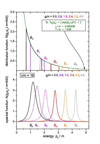
In Figure 11 (lower part) we present the spectral function for the initial distribution D2 at late times for various momentum modes as a function of the energy . – We note, that for all other initial distributions - with equal energy density - the spectral function looks very similar at this time since the systems proceed to the same stationary state (cf. Section 1.3). – We recognize that the spectral function is quite broad, especially for the low momentum modes, while for the higher momentum modes its width is slightly lower.
The distribution function as extracted from (34) is displayed in Fig. 11 (upper part) for the same momentum modes as a function of the energy . We find that for all momentum modes can be fitted by a single Bose-function with temperature . Thus the distribution function emerging from the Kadanoff-Baym time evolution for approaches a Bose function in the energy that is independent of the momentum as demanded by the equilibrium form (36).
Fig. 11 (upper part) demonstrates, furthermore, that the KMS-condition is fulfilled not only for on-shell energies, but for all . We, therefore, have obtained the full off-shell equilibrium state by integrating the Kadanoff-Baym equations in time. In addition, the limiting stationary state is the correct equilibrium state for all energies , i.e. also away from the quasi-particle energies.
We note in closing this Subsection, that the chemical potential – used as a second fit parameter – is already close to zero for these late times as expected for the correct equilibrium state of the neutral -theory that is characterized by a vanishing chemical potential in equilibrium which is actually achieved in the calculations for . This, at first sight, seems trivial but is a consequence of our ’exact’ treatment. In contrast, the Boltzmann equation (cf. Section 1.4) in general leads to a stationary state for with a finite chemical potential. We will attribute this failure of the Boltzmann approach to the absence of particle number nonconserving processes in the quasi-particle limit (see below).
1.4 Full versus approximate dynamics
The Kadanoff-Baym equations studied in the previous Sections represent the full quantum-field theoretical equations on the single-particle level. However, its numerical solution is quite involved and it is of strong interest to investigate, in how far approximate schemes deviate from the full calculation. Nowadays, transport models are widely used in the description of quantum systems out of equilibrium (cf. Introduction). Most of these models work in the ’quasi-particle’ picture, where all particles obey a fixed energy-momentum relation and the energy is no independent degree of freedom anymore; it is determined by the momentum and the (effective) mass of the particle. Accordingly, these particles are treated with their -function spectral shape as infinitely long living, i.e. stable objects. This assumption is very questionable e.g. for high-energy heavy ion reactions, where the particles achieve a large width due to the frequent collisions with other particles in the high-density and/or high-energy regime. Furthermore, this is doubtful for particles that are unstable even in the vacuum. The question, in how far the quasiparticle approximation influences the dynamics in comparison to the full Kadanoff-Baym calculation, is of widespread interest [53].
1.4.1 Derivation of the Boltzmann approximation
In the following we will give a short derivation of the Boltzmann equation starting directly from the Kadanoff-Baym dynamics in the two-time and momentum-space representation. This derivation is briefly reviewed since we want i) to emphasize the link of the full Kadanoff-Baym equation with its approximated version and ii) to clarify the assumptions that enter the Boltzmann equation.
Since the Boltzmann equation describes the time evolution of distribution functions for quasi-particles we first consider the quasi-particle Green-functions in two-time representation for homogeneous systems
| (37) | |||
where for each momentum the Green functions are freely oscillating in relative time with the on-shell energy . The time-dependent quasi-particle distribution functions are given with the energy variable fixed to the on-shell energy as , where the on-shell energies might depend on time as well. Such a time variation e.g. might be due to an effective mass as generated by the time-dependent tadpole self-energy. In this case the on-shell energy reads
| (40) |
Vice versa we can define the quasi-particle distribution function by means of the quasi-particle Green functions at equal times as
| (41) | |||||
Using the equations of motions for the Green functions in diagonal time direction (19) (exploiting the time evolution of the distribution function is given by
| (42) |
The time derivatives of the on-shell energies cancel out since the quasiparticle Green functions obey
| (43) |
as seen from (37). Furthermore, it is remarkable that contributions containing the energy - as present in the equation of motion for the Green functions (19) - no longer show up. The time evolution of the distribution function is entirely determined by (equal-time) collision integrals containing (time derivatives of the) Green functions and self-energies.
| (44) | |||||
Since we are dealing with a system of on-shell quasi-particles within the Boltzmann approximation, the Green functions in the collision integrals (44) are given by the respective quasi-particle quantities of (37). Moreover, the collisional self-energies (17) are obtained in accordance with the quasi-particle approximation as
| (45) | |||||
For a free theory the distribution functions are obviously constant in time which, of course, is no longer valid for an interacting system out of equilibrium. Thus one has to specify the above expressions for the quasi-particle Green functions (37) to account for the time dependence of the distribution functions.
The actual Boltzmann approximation is defined in the limit, that the distribution functions have to be taken always at the latest time argument of the two-time Green function [53]. Accordingly, for the general non-equilibrium case, we introduce the ansatz for the Green functions in the collision term
| (48) | |||||
with the maximum time . The same ansatz is employed for the time dependent on-shell energies which enter the representation of the quasi-particle two-time Green functions (48) with their value at , i.e. .
The collision term contains a time integration which extends from an initial time to the current time . All two-time Green functions and self-energies depend on the current time as well as on the integration time . Thus only distribution functions at the current time, i.e. the maximum time of all appearing two-time functions, enter the collision integrals and the evolution equation for the distribution function becomes local in time. Since the distribution functions are given at fixed time , they can be taken out of the time integral. When inserting the expressions for the self-energies and the Green functions in the collision integrals the evolution equation for the quasi-particle distribution function reads
| (49) | |||
where we have introduced the abbreviation for the distribution function at current time and for the according Bose factor. Furthermore, a possible time dependence of the on-shell energies is suppressed in the above notation.
The contributions in the collision term (49) for particles of momentum are ordered as they describe different types of scattering processes where, however, we always find the typical gain and loss structure. The first line in (49) corresponds to the production and annihilation of four on-shell particles (, ), where a particle of momentum is produced or destroyed simultaneous with three other particles with momenta . The second line and the forth line describe () and () processes where the quasi-particle with momentum is the single one or appears with two other particles. The relevant contribution in the Boltzmann limit is the third line which respresents () scattering processes; quasi-particles with momentum can be scattered out of their momentum cell by collisions with particles of momenta (second term) or can be produced within a reaction of on-shell particles with momenta , (first term).
The time evolution of the quasi-particle distribution is given as an initial value problem for the function prepared at initial time . For large system times (compared to the initial time) the time integration over the trigonometric function results in an energy conserving -function:
| (52) |
Here represents the energy sum which is conserved in the limit where the initial time is considered as fixed. In this limit the time evolution of the distribution function amounts to
| (53) | |||||
In the energy conserving long-time limit (52) only the scattering processes are non-vanishing, because all other terms do not contribute since the energy -functions can not be fulfilled for on-shell quasi-particles. Furthermore, the system evolution is explicitly local in time because it depends only on the current configuration; there are no memory effects from the integration over past times as present in the full Kadanoff-Baym equation.
In the following we will solve the energy conserving Boltzmann equation for on-shell particles:
| (54) | |||
The numerical algorithm employed for the solution of (54) is basically the same as for the solution of the Kadanoff-Baym equation (cf. Section 1.2). We explicitly calculate the time integral in (49). Energy conservation can be assured by a precalculation including a shift of the lower boundary to earlier times. We note, that in contrast to the Kadanoff-Baym equation no correlation energy is generated in the Boltzmann limit!
In addition to the procedure presented above we calculate the actual momentum-dependent on-shell energy for every momentum mode by a solution of the dispersion relation including contributions from the tadpole and the real part of the (retarded) sunset self energy. In this way one can guarantee that at every time the particles are treated as quasi-particles with the correct energy-momentum relation.
Before presenting the actual numerical results we comment on the derivation of the Boltzmann equation within the conventional scheme that is different from the one presented above. Here, at first the Kadanoff-Baym equation (in coordinate space) is transformed to the Wigner representation by Fourier transformation with respect to the relative coordinates in space and time. The problem then is formulated in terms of energy and momentum variables together with a single system time. For non-homogeneous systems a mean spatial coordinate is necessary as well. As a next step the ’semiclassical approximation’ is introduced, which consists of a gradient expansion of the convolution integrals in coordinate space within the Wigner transformation. For the time evolution only contributions up to first order in the gradients are kept. Finally, the quasi-particle assumption is introduced as follows: The Green functions appearing in the transport equation – explicitly or implicitly via the self-energies – are written in Wigner representation as a product of a distribution function and the spectral function . The quasi-particle assumption is then realized by employing a -like form for the spectral function which connects the energy variable to the momentum. By integrating the first order transport equation over all (positive) energies, furthermore, the Boltzmann equation for the time evolution of the on-shell distribution function (54) is obtained.
Inspite of the fact, that the Bolzmann equation (54) can be obtained in different subsequent approximation schemes, it is of basic interest, how its actual solutions compare to those from the full Kadanoff-Baym dynamics.
1.4.2 Boltzmann vs. Kadanoff-Baym dynamics
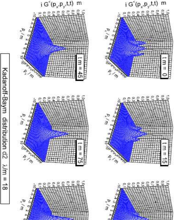
In the following we will compare the solutions of the Boltzmann equation with the solution of the Kadanoff-Baym theory. We start with a presentation of the non-equilibrium time evolution of two colliding particle accumulations (tsunamis) within the full Kadanoff-Baym calculation (see Figure 12).
During the time evolution the bumps at finite momenta (in direction) slowly disappear, while the one close to zero momentum – which initially stems from the vacuum contribution to the Green function – is decreased as seen for different snapshots at times 0, 15, 30, 45, 75, 150 in Fig. 12. The system with initially apparent collision axis slowly merges – as expected – into an isotropic final distribution in momentum space.
For the comparison between the full Kadanoff-Baym dynamics and the Boltzmann approximation we concentrate on equilibration times. To this aim we define a ’quadrupole’ moment for a given momentum distribution at time as
| (55) |
which vanishes for the equilibrium state. For the Kadanoff-Baym case we employ the actual distribution function by the relation
| (56) |
Note that when constructing the distribution function by means of equal-time Green functions the energy variable has been effectively integrated out. This has the advantage that the distribution function is given independently of the actual on-shell energies.
The relaxation of the quadrupole moment (56) has been studied for two different initial distributions: The evolution of distribution d2 is displayed in Fig. 12 while for distribution d1 the position and the width of the two particle bumps have been modified. The calculated quadrupole moment (56) shows a nearly exponential decrease with time (cf. Fig. 13) and one can extract a relaxation rate via the relation
| (57) |
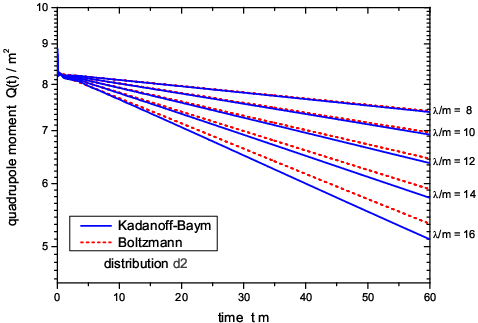
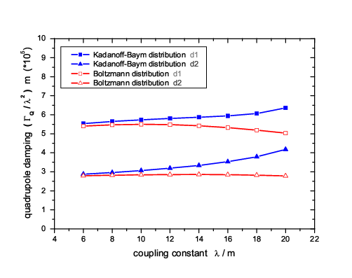
Fig. 14 shows for both initializations that the relaxation in the full quantum calculation occurs faster for large coupling constants than in the quasi-classical approximation, whereas for small couplings the equilibration times of the full and the approximate evolutions are comparable. We find that the scaled relaxation rate is nearly constant in the Boltzmann case, but increases with the coupling strength in the Kadanoff-Baym calculation (especially for initial distribution d2).
These findings are readily explained: Since the free Green function – as used in the Boltzmann calculation – has only support on the mass shell, only scattering processes are described in the Boltzmann limit. All other processes with a different number of incoming and outgoing particles vanish (as noted before). Within the full Kadanoff-Baym calculation this is different, since here the spectral function – determined from the self-consistent Green function – aquires a finite width. Thus the Green function has support at all energies although it drops fast far off the mass shell. Especially for large coupling constants, where the spectral function is sufficiently broad, the three particle production process gives a significant contribution to the collision integral. Since the width of the spectral function increases with the interaction strength, such processes become more important in the high coupling regime. As a consequence the difference between both approaches is larger for stronger interactions as observed in Fig. 14. For small couplings in both approaches basically the usual scattering contributes and the results for the thermalization rate are quite similar.
In summarizing this Subsection we point out that the full solution of the Kadanoff-Baym equations does include , and off-shell collision processes which – in comparison to the Bolzmann on-shell collision limit – become important when the spectral width of the particles reaches 1/3 of the particle mass. On the other hand, the simple Boltzmann limit works surprisingly well for smaller couplings and those cases, where the spectral function is sufficiently narrow.
2 Off-shell relativistic transport theory
Formal derivations of off-shell transport equations have been presented about 40 years ago by Kadanoff and Baym [13] but actual solutions have barely been addressed. This Section is devoted to a transparent derivation of generalized transport equations including numerical illustrations as well as detailed comparisons to the full theory.
2.1 Derivation of off-shell transport theory
The derivation of generalized transport equations starts by rewriting the Kadanoff-Baym equation for the Wightman functions in coordinate space () (8) as
| (58) |
The collision terms on the r.h.s. of (58) are given in space-time dimensions by convolution integrals over coordinate space self-energies and Green functions:
| (59) | |||||
In the general case of an arbitrary (scalar) quantum field theory is the local (non-dissipative) part of the path self-energy while resemble the non-local collisional self-energy contributions. In the representation (59) the integration boundaries are exclusively given for the time coordinates, while the integration over the spatial coordinates extends over the whole spatial volume from to in dimensions.
Since transport theories are formulated in phase-space one changes to the Wigner representation via Fourier transformation with respect to the rapidly varying (’intrinsic’) relative coordinate and treats the system evolution in terms of the (’macroscopic’) mean space-time coordinate and the four-momentum . The functions in Wigner space are obtained as
| (60) |
For the formulation of transport theory in the Wigner representation we have to focus not only on the transformation properties of ordinary two-point functions as given in (60), but also of convolution integrals as appearing in Eq. (59). A convolution integral in dimensions (for arbitrary functions ),
| (61) |
transforms as
| (62) | |||||
In accordance with the standard assumption of transport theory we assume that all functions only smoothly evolve in the mean space-time coordinates and thus restrict to first order derivatives. All terms proportional to second or higher order derivatives in the mean space-time coordinates (also mixed ones) will be dropped. Thus the Wigner transformed convolution integrals (61) are given in first order gradient approximation by,
| (63) |
using the relativistic generalization of the Poisson bracket
| (64) |
In order to obtain the dynamics for the spectral functions within
the approximate scheme we start with the Dyson-Schwinger equations
for the retarded and advanced Green functions in coordinate space
(14,15). – Note that the convolution
integrals in (14) and (15) extend over
the whole space and time range in contrast to the equations of
motion for the Wightman functions given in (58) and
(59)! – The further procedure consists in the
following steps: First we
i) transform the above equations into the Wigner representation
and apply the first order gradient approximation. In this limit
the convolution integrals yield the product terms and the general
Poisson bracket of the self-energies and the Green functions . We, furtheron, represent both
equations in terms of real quantities by the decomposition of the
retarded and advanced Green functions and self-energies as
We find that in Wigner space the real parts of the retarded and
advanced Green functions and self-energies are equal, while the
imaginary parts have opposite sign and are proportional to the
spectral function and the width ,
respectively. The next step consists in
ii) the separation
of the real part and the imaginary part of the two equations for
the retarded and advanced Green functions, that have to be
fulfilled independently. Thus we obtain four real-valued equations
for the self-consistent retarded and advanced Green functions. In
the last step
iii) we get simple relations by linear
combination of these equations, i.e. by adding/subtracting the
relevant equations.
This finally leads to two algebraic relations for the spectral function and the real part of the retarded Green function in terms of the width and the real part of the retarded self-energy as [64, 65]:
| (68) | |||||
| (69) |
Note that all terms with first order gradients have disappeared in (68) and (69). A first consequence of (69) is a direct relation between the real and the imaginary parts of the retarded/advanced Green function, which reads (for ):
| (70) |
Inserting (70) in (68) we end up with the following result for the spectral function and the real part of the retarded Green function
| (71) | |||||
| (72) |
where we have introduced the mass-function in Wigner space:
| (73) |
The spectral function (71) shows a typical Breit-Wigner shape with energy- and momentum-dependent self-energy terms. Although the above equations are purely algebraic solutions and contain no derivative terms, they are valid up to the first order in the gradients!
In addition, subtraction of the real parts and adding up the imaginary parts lead to the time evolution equations
| (74) | |||||
| (75) |
The Poisson bracket containing the mass-function leads to the well-known drift operator (for an arbitrary function ), i.e.
| (76) | |||||
| (77) |
such that the first order equations (74) and (75) can be written in a more comprehensive form as
| (78) | |||||
| (79) |
When inserting (71) and (72) we find that these first order time evolution equations are solved by the algebraic expressions. In this case the following relations hold:
| (80) | |||||
| (81) |
Thus we have derived the proper structure of the spectral function (71) within the first-order gradient (or semiclassical) approximation. Together with the explicit form for the real part of the retarded Green function (72) we now have fixed the dynamics of the spectral properties, which is consistent up to first order in the gradients.
2.1.1 Kadanoff-Baym transport
As a next step we rewrite the memory terms in the collision integrals (59) such that the time integrations extend from to . In this respect we consider the initial time whereas the upper time boundaries are taken into account by -functions, i.e.
| (82) |
We now perform the analogous steps as invoked before for the
retarded and advanced Dyson-Schwinger equations. We start with a
first order gradient expansion of the Wigner transformed
Kadanoff-Baym equation using (82) for the memory
integrals. Again we separate the real and the imaginary parts in
the resulting equation, which have to be satisfied independently.
At the end of this procedure we obtain a generalized transport
equation [13, 20, 24, 64, 65, 67, 69, 77]:
| (83) |
as well as a generalized mass-shell equation
| (84) |
with the mass-function specified in (73). Since the Green function consists of an antisymmetric real part and a symmetric imaginary part with respect to the relative coordinate , the Wigner transform of this function is purely imaginary. It is thus convenient to represent the Wightman functions in Wigner space by the real-valued quantities . Since the collisional self-energies obey the same symmetry relations in coordinate space and in phase-space, they will be kept also as furtheron.
In the transport equation (83) one recognizes on the l.h.s. the drift term , as well as the Vlasov term with the local self-energy and the real part of the retarded self-energy . On the other hand the r.h.s. represents the collision term with its typical ‘gain and loss’ structure. The loss term (proportional to the Green function itself) describes the scattering out of a respective phase-space cell whereas the gain term takes into account scatterings into the actual cell. The last term on the l.h.s. is very peculiar since it does not contain directly the distribution function . This second Poisson bracket vanishes in the quasiparticle approximation and thus does not appear in the on-shell Boltzmann limit. As demonstrated in detail in Refs. [13, 64, 65, 67, 69, 77] the second Poisson bracket governs the evolution of the off-shell dynamics for nonequilibrium systems.
Although the generalized transport equation (83) and the generalized mass-shell equation (84) have been derived from the same Kadanoff-Baym equation in a first order gradient expansion, both equations are not exactly equivalent [24, 64, 77]. Instead, they deviate from each other by contributions of second gradient order, which are hidden in the term (see below or Refs. [24, 77] for extended discussions). This raises the question: which one of these two equations has to be considered of higher priority? The question is answered in practical applications by the prescription of solving the generalized transport equation (83) for in order to study the dynamics of the nonequilibrium system in phase-space. Since the dynamical evolution of the spectral properties is taken into account by the equations derived in first order gradient expansion from the retarded and advanced Dyson-Schwinger equations, one can neglect the generalized mass-shell equation (84). Thus for our actual numerical studies in Section 2.2 we will use the generalized transport equation (83) supported by the algebraic relations (71) and (72).
2.1.2 Transport in the Botermans-Malfliet scheme
Furthermore, one recognizes by subtraction of the and mass-shell and transport equations, that the dynamics of the spectral function is determined in the same way as derived from the retarded and advanced Dyson-Schwinger equations (71) and (78). The inconsistency between the two equations (83) and (84) vanishes since the differences are contained in the collisional contributions on the r.h.s. of (83).
In order to evaluate the -term on the l.h.s. of (83) and to
explore the differences between the KB- and BM-form of the
transport equations (see below) it is useful to introduce
distribution functions for the Green functions and self-energies
as
| (85) | |||||
| (86) |
In equilibrium the distribution function with respect to the Green functions and the self-energies are given as Bose functions in the energy at given temperature; they thus are equal in equilibrium but in general might differ out-of-equilibrium. Following the argumentation of Botermans and Malfliet [24] the distribution functions and in (85) should be identical within the second term of the l.h.s. of (83) in order to obtain a consistent first order gradient expansion (without hidden higher order gradient terms). In order to demonstrate their argument we write
| (87) |
The ‘correction’ term
| (88) |
is proportional to the collision term of the generalized transport equation (83), which itself is already of first order in the gradients. Thus, whenever a distribution function appears within a Poisson bracket, the difference term ) becomes of second order in the gradients and should be omitted for consistency. As a consequence can be replaced by and thus the self-energy by in the Poisson bracket term . The generalized transport equation (83) then can be written in short-hand notation
| (89) |
with the mass-function (73). The transport equation (89) within the Botermans-Malfliet (BM) form resolves the discrepancy between the generalized mass-shell equation (84) and the generalized transport equation in its original Kadanoff-Baym (KB) form (83).
However, it is presently not clear in how far the generalized transport equations in KB-form (83) or in BM-form (89) reproduce the same dynamics as for the full Kadanoff-Baym theory (8). Moreover, the differences in the time evolution of nonequilibrium systems between the KB-form (83) and BM-form (89) are not known either. We will thus perform an explicit comparison between the different limits for -theory in 2+1 dimensions in the following Section.
2.2 Numerical studies on off-shell transport
In this Section we will perform numerical studies of the dynamics inherent in the generalized transport equations in comparison to solutions of the full Kadanoff-Baym equations (8) for the -theory in 2+1 space-time dimensions within the three-loop approximation for the effective action. This fixes the self-energies and in (83) and (84) to be the same as in the case of the full Kadanoff-Baym theory given by the tadpole (9) and the sunset (10) contributions, respectively.
For the first investigation we concentrate on the dynamics of the generalized transport equation (83). As in Section 1.2 we restrict ourselves to homogeneous systems in space. Consequently the derivatives with respect to the mean spatial coordinate vanish, such that the generalized transport equation (83) reduces to
| (90) |
with the simplified Poisson brackets (for arbitrary functions )
| (91) | |||
In order to obtain a numerical solution the Kadanoff-Baym equation (8) as well as the generalized transport equations (83) are transformed to momentum space. For the actual numerical integration of the generalized transport equation we will use the same grid in momentum space as employed for the full KB-theory in Section 1.2.
2.2.1 Phases of Equilibration
In order to specify the problem for the first order transport equation in time, the initial state has to be fixed, i.e., the initial Green function has to be specified for all momenta and all energies . According to (85) can be written as a product of a distribution function and a spectral function . In order to determine and we employ an iterative scheme: We first assume initial momentum-distribution functions equivalent to those used in the investigation of the full Kadanoff-Baym theory in Section 1.2 in order to allow for a comparison of the two schemes. These initial momentum distributions then fix on the time-diagonal axis by [72]
| (92) |
Next, the complete initial phase-space distribution function
in Wigner representation as well as
the spectral function is specified as a
function of the energy in an iterative way. As a starting
point we assume to be constant in the
energy variable . In order to determine the initial Green
function we employ the self-consistent iteration
procedure for the full spectral function as described in Appendix
D of Ref. [72] using the specified nonequilibrium
distribution function . The iteration process then yields
the fully self-consistent spectral function
for this initial distribution and
thus determines the initial Green function via
| (93) |
The advantage of the initialization prescription introduced above is that the actual spectral function – directly obtained by from the Green functions – complies with the one determined from the self-energies (71) in accordance with the first order gradient expansion scheme. During the nonequilibrium time evolution this correspondence is maintained since the analytic expression for the spectral function already is a solution of the generalized transport equation itself. Furthermore, the real part of the retarded Green function, that enters the peculiar second Poisson bracket on the l.h.s. in (83), can be taken in the first order scheme (72) which simplifies the calculations considerably.
Now we turn to the actual solutions of the generalized transport equation in the KB form (83). In Fig. 15 (left part) we show the time evolution of the equal-time Green function for the polar symmetric initial states D1, D2 and D3. Displayed are several momentum modes 0.0, 0.8, 1.6, 2.4, 3.2, 4.0 of the equal-time Green function on a logarithmic time scale. As in the full Kadanoff-Baym theory (right part) one finds that for all initializations the quantum system approaches a stationary state for , i.e. all momentum modes approach a constant.


However, the respective momentum modes of the different initializations do not achieve identical values for , as seen in particular for the low momenta 0.0, 0.8 in Fig. 15 (left part). This is not surprising since the various initializations – obtained within the self-consistent scheme described above – do not correspond to exactly the same energy. This is why the respective long-time limits differ slightly. The small difference in energy is, of course, most prominently seen in the low momentum (energy) modes. Moreover, the dynamics within the generalized transport equation (83) is in general very similar to the full Kadanoff-Baym theory (right part). For all three initial states we find (apart from the very initial phase 5) the same structures during the equilibration process. In particular for the initializations D1 and D2 the characteristic overshooting for the low momentum modes is seen as in the full quantum evolution, which does not show up in solutions of the corresponding on-shell Boltzmann limit. Since in the Boltzmann limit a strictly monotonous evolution of the momentum modes is seen (cf. Ref. [72]) this overshooting has to be attributed to an off-shell quantum effect. Even the positions of the maxima are in a comparable range: For the initialization D1 they are shifted to slightly larger times and are a little bit lower than in the full calculation; the same holds for the initial state D2. The initial distribution D3 yields a monotonous behaviour for all momentum modes within the generalized transport formulation which is again in a good agreement with the full dynamics.
Some comments are worthwhile with respect to the comparison performed above: The spectral function in the Kadanoff-Baym calculation is completely undetermined in the initial state; it develops during the very early phase to an approximate form (which in the following still evolves in time). In contrast to this, the spectral function in the generalized transport formulation (83) has a well-defined structure already from the beginning. This principle difference results from the fact, that in the Kadanoff-Baym case we deal with a true initial value problem in the two time directions (). Additionally, the relative time integral in () – to obtain the spectral function in energy by Wigner transformation – is very small. Consequently, the spectral shape in Wigner space is determined by the finite integration interval in time rather than by the interactions itself. On the other hand, we have used an infinite relative time range in deriving the generalized transport equation within the first order gradient expansion. Thus in this case we deal with a completely resolved spectral function already at the initial time! This demonstrates why both approaches can only be compared to a limited extent for the very early times!
Finally, concentrating on the very early time behaviour, we find a significant difference between the full and the approximate dynamics in the gradient scheme (83). For the generalized transport equation we observe a monotonous evolution of the equal-time Green function momentum modes whereas strong oscillations are seen in the initial phase for the solution of the full Kadanoff-Baym theory. Thus – with respect to the early time behaviour – the generalized transport equation behaves much more like the Boltzmann approximation, which is a first order differential equation in time as well. However, the Kadanoff-Baym evolution is given by an integro-differential equation of second order in time. In this case the phase correlations between the Green functions are kept and the instantaneous switching-on of the interaction results in an oscillatory behaviour of the single momentum modes.
2.2.2 Evolution of the Spectral Function

Since the Green functions develop in time also the spectral properties of the system change as well. In Fig. 16 the time evolution of the spectral functions for the initializations D1, D2 and D3 within the gradient scheme are displayed for two particular momentum modes 0.0 (l.h.s.) and 2.0 (r.h.s.) for various system times 5, 20, 60, 120, 240, 360, 480, 600 up to the long-time limit. This representation corresponds to Fig. 8, where the respective evolution of the spectral function is studied for the full Kadanoff-Baym theory. We find that the time evolution of the spectral functions obtained from the generalized transport equation (83) is very similar to the one from the full quantum calculation (see below). The zero-mode spectral function for the initial distribution D1 becomes sharper with time and is moving to slightly higher energies. The opposite characteristics is observed for the zero-mode spectral function for the initialization D3, which broadens with time (reducing the peak correspondingly) and slowly shifts to smaller energies. Together with the weak evolution for the distribution D2 (which only slightly broadens at intermediate times and returns to a narrower shape at smaller energies in the long-time limit) the evolution of all three initializations in the semiclassical approximation is well comparable to the full Kadanoff-Baym dynamics (cf. Fig. 8). Furthermore, the maxima of the zero-mode spectral functions are located above the bare mass (as indicated by the on-shell arrow) for all initial states during the time evolution.


The spectral functions for the momentum mode 2.0 are in a good agreement with the Kadanoff-Baym dynamics as well. Again we observe – for the initial distribution D1 – a narrowing of the spectral function, while for D3 the spectral function broadens with time. Moreover, the width of the spectral function starting from distribution D2 shows a non-monotonous behaviour with a maximum at intermediate times.
In order to study the dynamics of the spectral function in a more quantitative manner we display in Fig. 17 the time evolution of the on-shell energies (as derived from the maxima of the spectral function) for the momentum modes 0.0 (upper plot) and 2.0 (lower plot) for the initializations D1, D2 and D3 with 18 (l.h.s.). By comparison with the corresponding results from the Kadanoff-Baym theory (r.h.s.) we observe a close similarity of the evolutions within the full and the semiclassical KB scheme. The effective mass of the zero momentum mode decreases for initialization D3, passes a minimum for D2 and increases for the initial state D1.
As familiar from the Kadanoff-Baym calculations in Section 1.2 the behaviour of the on-shell energies is different for higher momentum modes. We find for the momentum mode 2.0 a monotonous decrease of the on-shell energy for the initializations D1 and D2 and an increase for distribution D3. Altogether, the evolution of the on-shell energies for the higher modes is rather moderate compared to the lower ones in accordance with the dominant momentum contribution and the weakening of the retarded self-energy for higher energy modes.
Finally, the on-shell energies approach a stationary state for all modes and all initializations. However, the long-time limit of the equal momentum modes is not exactly the same for all initial distributions D1, D2 and D3. As discussed above this small difference can be traced back to the specific initial state generation from the given momentum distribution.
Next we consider the time evolution of the on-shell width as determined by the imaginary part of the retarded self-energy at the maximum position of the spectral function. In Fig. 18 (l.h.s.) the on-shell width is displayed for the two momentum modes 0.0 and 2.0 for all three initial distributions D1, D2 and D3 with 18 as a function of time. For both momentum modes the on-shell width increases for the distribution D3, while it has a maximum at intermediate times ( 40) for the initialization D2. Thus the results – together with the reduction of the on-shell width for both momentum modes for the initialization D1 – is in good agreement with the results obtained for the full Kadanoff-Baym theory (r.h.s.). However, the stationary values for the on-shell widths deviate again slightly in accordance with the different preparation of the initial state in the gradient scheme.
In summarizing we find that the main characteristics of the full quantum evolution of the spectral function are maintained in the semiclassical transport equation (83) as well. This includes the evolution of the on-shell energies as well as the width of the spectral function. Since the generalized transport equation is formulated directly in Wigner space one has access to the spectral properties at all times, whereas the very early times in the Kadanoff-Baym case have to be excluded due to the very limited support in the relative time interval () for the Wigner transformation.
2.2.3 Stationary State of the Semiclassical Evolution


As we have observed in the previous Subsections the evolution within the generalized transport equation (83) leads to a stationary state for all three different initializations D1, D2 and D3. Thus we turn to the investigation of this long-time limit itself, here in particular for the initialization D2. In Fig. 19 (l.h.s.) we show the distribution function of various momentum modes 0.0, 0.8, 1.6, 2.4, 3.2, 4.0 for large times ( = 600) as derived from the Green function itself and the spectral function via the relation . The distribution function for a given momentum mode is calculated for all energies where the corresponding spectral function – as displayed in the lower part of Fig. 19 – exceeds a value of 0.5. Since the width of the late time spectral function decreases with increasing momentum, the energy range (for which the distribution function is shown), is smaller for larger momentum modes. We find, that all momentum modes of can be fitted at all energies by a single Bose function with a temperature 1.827 and a very small chemical potential 0.000817. Thus the generalized transport formulation (83) leads to a complete (off-shell) equilibration of the system very similar to the solution of the full Kadanoff-Baym equation (r.h.s. of Fig. 19). Furthermore, the long-time limit of the semiclassical time evolution exhibits a vanishing chemical potential in accordance with the properties of the neutral -theory. This might have been expected since in the generalized transport equation particle number non-conserving processes of the type – which lead to the decrease of the chemical potential – are included by means of the dynamical spectral function. Thus the semiclassical approximation (83) solves the problems within the Boltzmann limit, which does not yield a relaxation of the chemical potential, since only on-shell transitions of quasiparticles are taken into account as demonstrated in Section 1.4.
After observing, that the chemical potential decreases to zero in the long-time limit, it is interesting to study the relaxation process itself. The relaxation of the chemical potential for the three different initializations D1, D2 and D3 (with coupling constant 18) shows an approximately exponential decrease in time. The relaxation rates – as determined from the slope of the exponential decline – are also approximately the same for all distributions. They are given explicitely by for distribution D1, for distribution D2 and for distribution D3. Thus the relaxation rates are in the same range as those found within the full Kadanoff-Baym theory (Section 1.3).
We conclude that – although there is a small relative shift of the different time scales of kinetic and chemical equilibration as a function of the coupling strength with respect to the full KB solutions – the results of the generalized KB transport equations are very similar. The differences we attribute to higher-order multi-particle effects in off-shell transitions. While the kinetic equilibration proceeds approximately with the coupling constant squared (as indicated by the calculations for non-polar-symmetric systems), the chemical relaxation rate is a higher order process in the coupling constant .
2.2.4 Quadrupole Relaxation
In this Subsection we no longer restrict to polar symmetric systems and discuss the time evolution of more general initial distributions within the generalized transport approximation (83). We start with conditions similar to those employed in Section 1.4 but combined with the initialization scheme for the semiclassical limit. Again the decrease of the quadrupole moment of the distribution
| (94) |
is approximately exponential in time () and thus allows for the extraction of a quadrupole damping rate . The scaled quadrupole damping rates – as obtained for the two initial distributions D1 and D2 – are displayed in Fig. 20 as a function of the coupling strength .

The calculations show that the quadrupole relaxation rates within the semiclassical approximation (83) for both initial distributions D1 and D2 is well within in the range of the full Kadanoff-Baym and the on-shell Boltzmann case. Additionally, the quadrupole relaxation rate is rather flat in the coupling when divided by the coupling constant squared () as already observed for the other two evolution schemes in Section 1.4. Nevertheless, the relaxation in the full KB-theory (8) proceeds slightly faster than in the transport limits for large couplings. The latter effect is again attributed to higher order off-shell transition effects which are no longer incorporated in the generalized KB transport equation.
2.2.5 Kadanoff-Baym versus Botermans-Malfliet transport
In this Subection we will perform a comparison of the generalized transport equation in the original Kadanoff-Baym (KB) form (83) with the modified Botermans-Malfliet (BM) form (89). As discussed in detail in Section 2.1.2 the latter form results from the replacement of the collisional self-energy by
| (95) |
in the second Poisson bracket on the l.h.s. of the original kinetic equation (83). This replacement leads to a consistent first order equation in the gradients and achieves consistency of the resulting transport equation with the corresponding generalized mass-shell relation (84). As noted before, the replacement (95) might be questionable in the general case; thus explicit numerical investigations are needed.

In Fig. 21 we compare the time evolution within the generalized transport equation in the KB form to the consistent equation in BM form. In this respect several momentum modes of the equal-time Green function are displayed evolving in time from an initial distribution D2 for a coupling constant 16. We find that the deviations between both approximations (KB and BM) are rather moderate. Only for very small momentum modes 1.6 deviations between both modes are visible. For the very low momentum modes the range of difference starts at 10 and extends to 100 for the non-zero modes. For the zero momentum mode the deviation lasts even longer. In this region the semiclassical transport in the BM form is slightly ’slower’ than in the original KB choice. Nevertheless, also the BM form exhibits the typical overshooting behaviour of the low momentum modes beyond the stationary limit as observed for the KB form. However, the maxima are shifted slightly to later times. Finally, both gradient approximations converge in the long-time limit to very similar configurations.
In summarizing we point out that the approximation of the full Kadanoff-Baym dynamics by the generalized transport equations in Kadanoff-Baym (83) or Botermans-Malfliet form (89) holds very well for the different momentum modes of the Green function itself. Slight deviations are only visible for the zero momentum mode at early to intermediate times (Figs. 15 and 21) for a logarithmic representation of the time axis. Consequently, the characteristic features of quantum equilibration obtained for the full Kadanoff-Baym theory are retained in the generalized transport limits.
2.3 Testparticle representation
The generalized transport equation (89) allows to extend the traditional on-shell transport approaches for which efficient numerical recepies have been set up [29, 78, 79, 80, 81, 82, 83, 84, 85, 86, 87, 88, 89, 90, 91] (and Refs. therein). In order to obtain a practical solution to the transport equation (89) we use a testparticle ansatz for the Green function , more specifically for the real and positive semidefinite quantity
| (96) |
In the most general case (where the self energies depend on four-momentum , time and the spatial coordinates ) the equations of motion for the testparticles read [65]
| (97) | |||||
| (98) | |||||
| (99) |
where the notation implies that the function is taken at the coordinates of the testparticle, i.e. .
In (97-99) a common multiplication factor appears, which contains the energy derivatives of the retarded self energy
| (100) |
It yields a shift of the system time to the ’eigentime’ of particle defined by . As the reader immediately verifies, the derivatives with respect to the ’eigentime’, i.e. , and then emerge without this renormalization factor for each testparticle when neglecting higher order time derivatives in line with the semiclassical approximation scheme.
Some limiting cases should be mentioned explicitly: In case of a momentum-independent ’width’ we take as an independent variable instead of , which then fixes the energy (for given and ) to
| (101) |
Eq. (99) then turns to ()
| (102) |
for the time evolution of the test-particle in the invariant mass squared. In case of the familiar equations of motion for testparticles in on-shell transport approaches are regained.
2.3.1 Model simulations for the momentum-dependent transport equations in testparticle representation
To demonstrate the physical content of the equations of motion for testparticles (97-99) we perform an exploratory study with a momentum-dependent trial potential. The potential is chosen of the type:
| (103) |
with a constant (but finite) vacuum width . While the spatial extension of the potential is given by a Woods-Saxon shape (with parameters fm and fm) its momentum dependence for the real as well as for the imaginary part is introduced by
| (104) |
Here the constants () give the ’strength’ of the complex potential while () play the role of cutoff-parameters. Due to the structure in the denominator of (104) the momentum-dependent part of this potential is explicitly Lorentz-covariant but should be considered for .
In the simulations the testparticles are propagated with different initial mass parameters , which are shifted relative to each other by [GeV] around a mean mass of 1.0 GeV. To each testparticle a momentum in positive -direction is attributed so that all of them have initially the same energy = 2.0 GeV. All testparticles are initialized on the negative -axis with ( fm) and then evolved in time according to the equations of motion (97-99).


In our first simulation we consider a purely imaginary potential with a strength of GeV2 and a cutoff-parameter GeV. The evolution in energy , momentum and in the mass parameter for all testparticles is shown in Fig. 22 (l.h.s., upper part) as a function of . When the testparticles enter the potential region, their momenta and mass parameters are modified. The imaginary potential leads to a spreading of the trajectories in the mass parameter which in turn reflects a broadening of the spectral function. The relation between the imaginary self energy and the spreading in mass is fully determined by relation (102). Since we have chosen a potential with no explicit time dependence the energy of each testparticle is a constant of time. According to the explicit momentum dependence of our ’trial’ potential each single testparticle is affected with different strength. Since the imaginary potential is strongest for small momenta (which correspond to the highest lines in the lower graph of Fig. 22) (l.h.s.) the momentum and mass coordinates of those testparticles are changed predominantly that are initialized with the lowest momenta (i.e. with the largest masses). As a result one observes a rather asymmetric distribution in the mass parameters (and in the momenta) in the potential zone. For the mass and momentum coordinates of the testparticles regain the proper asymptotic value.
In the second example we allow for an addititonal real part of the self energy. The calculation is performed with the parameters GeV2, GeV2 and GeV. The momentum-dependent real part (r.h.s., lower part of Fig. 22) causes an additional shift of the testparticle momenta. Since the real part of the potential is larger for small initial momenta, these testparticle momenta are shifted up somewhat more than for particles with larger momenta. This gives rise to a reduction of the asymmetry which was introduced by the momentum-dependent imaginary part of the self energy (r.h.s., upper part of Fig. 22). The mass parameters of the testparticles are only weakly influenced by the real part of the potential.

We, furthermore, study the implications of the correction term using the same imaginary potential as in Fig. 22. The time evolution of the correction factor for each testparticle is displayed in the lower part of Fig 23. While it is for large initial mass parameters , it is for mass parameters . In the upper part of Fig. 23 the momenta of the testparticles are shown for two calculational limits: in the first one the correction term is taken into account (as in the previous calculations), while in the second one the corrections due to the energy dependence of the retarded self energy are neglected. However, the calculations with and without the correction factor exhibit no difference in the testparticle momenta as a function of . The same holds for the mass parameters which are not displayed here since they provide no new information due to energy conservation. We thus conclude that the particle trajectory (in phase space) is independent of these correction factors, since the correction term – when displayed as in phase-space – leads only to a rescaling of the ’eigentime’ of the testparticles as pointed out above.
2.3.2 Collision terms
The collision term of the Kadanoff-Baym equation can only be worked out in more detail by giving explicit approximations for and . A corresponding collision term can be formulated in full analogy to Refs. [79, 92], e.g. from Dirac-Brueckner theory (cf. also Section 1.2), following detailed balance as
| (105) |
with
| (106) |
and for bosons/fermions, respectively. The indices stand for the antisymmetric/symmetric matrix element of the in-medium scattering amplitude in case of fermions/bosons. In Eq. (105) the trace over particles 2,3,4 reads explicitly for fermions
| (107) |
where denote the spin and isospin of particle 2. In case of bosons we have
| (108) |
since here the spectral function is normalized as
| (109) |
whereas for fermions we have
| (110) |
We mention that the spectral function in case of fermions in (105) is obtained by considering only particles of positive energy and assuming the spectral function to be identical for spin ’up’ and ’down’ states. In general, the spectral function for fermions is a Dirac-tensor with denoting the Dirac indices. It is normalized as
| (111) |
which implies
| (112) |
Now expanding in terms of free spinors (=1,2) and as
| (113) |
one can separate particles and antiparticles. By neglection of the antiparticle contributions (i.e. ) and within the assumption that the spectral function for the particles is diagonal in spin-space (i.e. ) as well as spin symmetric, one can define as
| (114) |
Neglecting the ’gain-term’ in eq. (105) one recognizes that the collisional width of the particle in the rest frame is given by
| (115) |
where – as in eq. (105) – local on-shell scattering processes are assumed for the transitions . We note that the extension of eq. (105) to inelastic scattering processes (e.g. ) or ( etc.) is straightforward when exchanging the elastic transition amplitude by the corresponding inelastic one and taking care of Pauli-blocking or Bose-enhancement for the particles in the final state.
For particles of infinite life time in vacuum – such as protons – the collisional width (115) has to be identified with twice the imaginary part of the self energy. Thus the transport approach determines the particle spectral function dynamically via (115) for all hadrons if the in-medium transition amplitudes are known in their full off-shell dependence. Since this information is not available for configurations of hot and dense matter, which is the major subject of future development, a couple of assumptions and numerical approximation schemes have to be invoked in actual applications.
3 The dynamical quasiparticle approach to hot QCD
This Section addresses the question how to achieve a suitable approximation for the spectral functions of partons (quarks and gluons) in hot QCD, i.e. at temperatures above the deconfinement transition . Since the spectral functions are fully determined by complex selfenergies for the partons, it is sufficient to determine effective selfenergies, e.g., from lattice QCD.
3.1 Application to parton dynamics
The ’Big Bang’ scenario implies that in the first micro-seconds of the universe the entire system has emerged from a partonic system of quarks, antiquarks and gluons – a quark-gluon plasma (QGP) – to color neutral hadronic matter consisting of interacting hadronic states (and resonances) in which the partonic degrees of freedom are confined. The nature of confinement and the dynamics of this phase transition has motivated a large community for several decades (cf. [93, 94] and Refs. therein). Early concepts of the QGP were guided by the idea of a weakly interacting system of partons since the entropy density and energy density were found in lattice QCD to be close to the Stefan Boltzmann (SB) limit for a relativistic noninteracting system [95]. However, experimental observations at the Relativistic Heavy Ion Collider (RHIC) indicated that the new medium created in ultrarelativistic Au+Au collisions was interacting more strongly than hadronic matter and consequently this notion had to be given up. Moreover, in line with earlier theoretical studies in Refs. [96, 97, 98] the medium showed phenomena of an almost perfect liquid of partons [99, 100] as extracted from the strong radial expansion and elliptic flow of hadrons as well the scaling of the elliptic flow with parton number etc. All the latter collective observables have been severely underestimated in conventional string/hadron transport models [101, 102, 103] whereas hydrodynamical approaches did quite well in describing (at midrapidity) the collective properties of the medium generated during the early times for low and moderate transverse momenta [104, 105]. The question about the constituents and properties of this QGP liquid is discussed controversely in the literature (cf. Refs. [106, 107, 108]) and practically no dynamical concepts are available to describe the dynamical freezeout of partons to color neutral hadrons that are finally observed experimentally. Since the partonic system appears to interact more strongly than even hadronic systems the notation strong QGP (sQGP) has been introduced in order to distinguish from the dynamics known from perturbative QCD (pQCD).
Lattice QCD (lQCD) calculations provide some guidance to the thermodynamic properties of the partonic medium close to the transition at a critical temperature up to a few times , but lQCD calculations for transport coefficients presently are not accurate enough [109] to allow for firm conclusions. Furthermore, it is not clear whether the partonic system really reaches thermal and chemical equilibrium in ultrarelativistic nucleus-nucleus collisions [110] such that nonequilibrium models are needed to trace the entire collision history. The available string/hadron transport models [81, 82, 111] partly fail - as pointed out above - nor do partonic cascade simulations [112, 113, 114, 115] (propagating massless partons) sufficiently describe the reaction dynamics when employing cross sections from perturbative QCD. Some models, e.g. the Multiphase Transport Model AMPT [116], employ strong enhancement factors for the cross sections, however, use only on-shell massless partons in the partonic phase as in Ref. [113]. The same problem comes about in the parton cascade model of Ref. [117] where additional 2 3 processes like are incorporated but massless partons are involved.
On the other hand it is well known that strongly interacting quantum systems require descriptions in terms of propagators with sizeable selfenergies for the relevant degrees of freedom (cf. Sections 1 and 2). While the real part of the selfenergies can be related to mean-field potentials, the imaginary parts provide information about the lifetime and/or reaction rate of time-like ’particles’ [118]. The studies of Peshier [119, 120] indicate that the effective degrees of freedom in a partonic phase should have a width in the order of the pole mass already slightly above . This opens up the problem how to interpret/deal with the space-like part of the distribution functions and how to ’propagate’ effective degrees in space-time in equilibrium as well as out of equilibrium without violating ’microcausality’. These questions will now be addressed in the Dynamical QuasiParticle Model (DQPM) [121].
3.2 Off-shell elements in the DQPM
The dynamical quasiparticle model goes back to Peshier [119, 120] and starts with the entropy density in the quasiparticle limit [120, 122, 123, 124],
| (116) |
where and denote the Bose and Fermi distribution functions, respectively, while , and stand for the full (scalar) quasiparticle propagators of gluons , quarks and antiquarks . The degeneracy factor for gluons is = 16 while for quarks and antiquarks we get = 18 for three flavors . In Eq. (116) and denote the (retarded) quasiparticle selfenergies. In principle, as well as are Lorentz tensors and should be evaluated in a nonperturbative framework. The DQPM treats these degrees of freedom as independent scalar fields with scalar selfenergies. In case of the fermions and (for and ) have Lorentz scalar and vector contributions but only scalar terms are kept in (116) for simplicity which are assumed to be identical for quarks and antiquarks. Note that one has to treat quarks and antiquarks separately in (116) as their abundance differs at finite quark chemical potential .
Since the nonperturbative evaluation of the propagators and selfenergies in QCD is a formidable task (and addressed in Dyson-Schwinger (DS) Bethe-Salpeter (BS) approaches [125, 126, 127, 128, 129]) an alternative and practical procedure is to use physically motivated Ansätze with Lorentzian spectral functions for quarks22 2 In the following the abbreviation is used that ’quarks’ denote quarks and antiquarks if not specified explicitly. and gluons,
| (117) |
and to fit the few parameters to results from lQCD. With the convention , the parameters and are directly related to the real and imaginary parts of the corresponding (retarded) self-energy, e.g. in case of the ’scalar’ gluons.
Following [120] the quasiparticle mass (squared) for gluons is assumed to be given by the thermal mass in the asymptotic high-momentum regime, i.e.
| (118) |
and for quarks (assuming vanishing constituent masses here) as,
| (119) |
with a running coupling (squared),
| (120) |
which permits for an enhancement near [130, 131, 132]. Here stands for the number of colors while denotes the number of flavors and the quark chemical potentials. The parameters and have been fixed in Ref. [120]. As demonstrated in Fig. 24 this functional form for the strong coupling is in accordance with the lQCD calculations of Ref. [133] for the long range part of the potential.

The width for gluons and quarks (for ) is adopted in the form [134]
| (121) |
where (from Ref. [97]) is related to a magnetic cut-off.
The physical processes contributing to the width are both , scattering as well as splitting and fusion reactions , , or etc. On the fermion side elastic fermion-fermion scattering , where stands for a quark or antiquark , fermion-gluon scattering , gluon bremsstrahlung or quark-antiquark fusion etc. emerge. Note, however, that the explicit form of (121) is derived for hard two-body scatterings only. It is worth to point out that the ratio of the masses to their widths approaches zero only asymptotically for such that the width of the quasiparticles is comparable to the pole mass slightly above up to all terrestrial energy scales.
Within the DQPM the real and imaginary parts of the propagators and now are fixed and the entropy density (116) can be evaluated numerically once the free parameters in (120) are determined. In the following we will assume 3 light quark flavors . Since the presently available unquenched lQCD calculations (for three flavors) for the entropy density are still accompanied with rather large error bars the parameters of the DQPM are taken the same as in the pure Yang-Mills sector: , as determined in Refs. [97, 120]. This is legitimate since an approximate scaling of thermodynamic quantities from lQCD is observed when dividing by the number of degrees of freedom and scaling by the individual critical temperature which is a function of the different number of parton species [135]. However, these parameters will have to be refitted once more accurate ’lattice data’ become available.
The resulting values for the gluon and quark masses - multiplied by - are displayed in Fig. 25 (for ) by the solid lines while the gluon and quark width ( - multiplied by - are displayed in terms of the dashed lines as a function of . The actual numbers imply very ’broad’ quasiparticles already slightly above . For the ratio =4/9 is the same as for the ratio of the squared masses and reflects the ratio of the Casimir eigenvalues in color space. Consequently the ratio of the width to the pole mass is smaller for quarks (antiquarks) than for gluons in the whole temperature range.

In order to fix the scale , which is not specified so far, one may directly address unquenched lQCD calculations (for 3 light flavors). However, here the situation is presently controversal between different groups (cf. Refs. [136, 137] and the discussion therein). An alternative way is to calculate the pressure from the thermodynamical relation (at = 0),
| (122) |
by integration of the entropy density over , where one may tacitly identify the ’full’ entropy density with the quasiparticle entropy density (116). Since for the DQPM entropy density drops to zero (with decreasing ) due to the high quasiparticle masses and the width vanishes as well (cf. Fig. 25) the integration constant may be assumed to be zero in the DQPM which focusses on the quasiparticle properties above .

The energy density then follows from the thermodynamical relation [130, 138]
| (123) |
(for = 0) and thus is also fixed by the entropy as well as the interaction measure
| (124) |
that vanishes for massless and noninteracting degrees of freedom.
The actual results for are displayed in Fig. 26 (solid violet line), (blue dash-dotted line) as well as the interaction measure (124) (green dotted line) and show the typical pattern from lQCD calculations [135]. The scale may now be fixed (estimated) by requiring that the critical energy density is roughly the same for the pure Yang-Mills case as for the full theory with dynamical quarks in line with the approximate scaling of lQCD [135]. Since in the Yang Mills sector is about 1 GeV/fm3 (cf. [121]) the scaled energy density from Fig. 26 can be employed to fix the critical temperature 0.185 GeV. This leads to the ’thumb rule’ [GeV/fm3] for which is roughly fulfilled according to Fig. 26.

A first test of the DQPM in comparison to lQCD calculations is given for the sound velocity (squared),
| (125) |
which does not depend on the absolute (uncertain) scale of . This comparison is shown in Fig. 27 by the solid line where the lQCD results have been taken from Ref. [139] and correspond to with . The DQPM is seen to reproduce the drop in close to within errorbars and to reach the asymptotic value = 1/3 approximately for . This comparison, however, has to be taken with some care since the present DQPM assumes massless current quarks whereas the lQCD calculations employ finite quark masses.
3.2.1 Time-like and space-like quantities
For the further analysis of the DQPM it is useful to introduce the shorthand notations
| (126) |
with denoting the invariant mass squared. The quark and antiquark degrees of freedom, i.e. 2 = 36, are by roughly a factor of two more abundant than the gluonic degrees of freedom. The function in (126) separates time-like quantities from space-like quantities and can be inserted for any observable of interest. Note, however, that not all space-like quantities have a direct physical interpretation!
We note in passing that the entropy density (116) is dominated by the time-like contributions for quarks and gluons and shows only minor space-like parts (cf. Refs. [120, 121]). Furthermore, the entropy density from the DQPM is only 10 - 15 smaller than the Stefan Boltzmann entropy density for as in the case of lQCD [95].
Further quantities of interest are the ’quasiparticle densities’
| (127) |
that correspond to the time-like (+) and space-like (-) parts of the integrated distribution functions. Note that only the time-like integrals over space have a particle number interpretation. In QED this corresponds e.g. to time-like photons () which are virtual in intermediate processes but may also be seen asymptotically by dileptons (e.g. pairs) due to the decay [111, 140] (cf. Section 4).
Scalar densities for quarks and gluons - only defined in the time-like sector - are given by
| (128) |
and have the virtue of being Lorentz invariant.
Before coming to the actual results for the quantities (127) and (128) it is instructive to have a look at the integrand in the quark density (127) which reads as (in spherical momentum coordinates with angular degrees of freedom integrated out)
| (129) |
Here the integration is to be taken over and from to . The integrand is shown in Fig. 28 for (l.h.s.) and (r.h.s.) () in terms of contour lines spanning both one order of magnitude. For the lower temperature the quark mass is about 0.55 GeV and the width 0.034 GeV such that the quasiparticle properties are close to an on-shell particle. In this case the integrand is essentially located in the time-like sector and the integral over the space-like sector is almost negligible. This situation changes for where the mass is about 0.7 GeV while the width increases to 0.25 GeV. This situation is close to the systems studied in Sections 1 and 2 in case of -theory and a strong coupling ( 18). As one observes from the r.h.s. of Fig. 28 the maximum of the integrand is shifted towards the line and higher momentum due to the increase in temperature by about a factor of three; furthermore, the distribution reaches far out in the space-like sector due to the Fermi factor which favors small . Thus the relative importance of the time-like (+) part to the space-like (-) part is dominantly controlled by the width - relative to the pole mass - which determines the fraction of with negative invariant mass squared relative to the time-like part ().

The actual results for the different ’densities’ (multiplied by ) are displayed in Fig. 29 for gluons (l.h.s.) and quarks (r.h.s.) including the antiquarks. The lower (magenta) lines represent the scalar densities , the red solid lines the time-like densities , the green lines the quantities while the thick solid blue lines are the sum as a function of (assuming = 0.185 GeV). It is seen that is substantially smaller than in case of gluons in the temperature range 1.1 10. The quantity follows closely the Stefan Boltzmann limit for a massless noninteracting system of bosons which is given in Fig. 29 (l.h.s.) by the upper dash-dotted line. Though differs by less than 20% from the Stefan Boltzmann (SB) limit for the physical interpretation is essentially different! Whereas in the SB limit all gluons move on the light cone without interactions only a small fraction of gluons can be attributed to quasiparticles with density within the DQPM that propagate within the lightcone. The space-like part corresponds to ’gluons’ exchanged in -channel scattering processes and thus cannot be propagated explicitly in off-shell transport approaches without violating causality and/or Lorentz invariance. In case of quarks (or antiquarks) the results are qualitatively similar but now the time-like part comes closer to the space-like part since the ratio of the width to the pole mass () is smaller than the corresponding ratio for gluons as stated above. Furthermore, the quantity is closer to the respective SB limit (for massless fermions) due to the lower effective mass of the quarks. In this respect the quarks and antiquarks are closer to (but still far from) the massless on-shell quasiparticle limit.

The scalar densities (lower magenta lines) follow smoothly the time-like densities (for gluons as well as quarks+antiquarks) as a function of temperature and uniquely relate to the corresponding time-like densities or the temperature in thermal equilibrium.
The separation of and so far has no direct dynamical implications except for the fact that only the fraction can explicitly be propagated in transport models as argued above. Following Ref. [121] we, furthermore, consider the energy densities,
| (130) |
that specify time-like and space-like contributions to the quasiparticle energy densities ().

The result for the quasiparticle energy densities and are displayed in Fig. 30 for gluons (l.h.s.) and quarks+antiquarks (r.h.s.) as a function of . All quantities have been multiplied by the dimensionless factor in order to divide out the leading temperature dependence. The lower red solid lines show the time-like components while the dashed green lines display the space-like parts which dominate over the time-like parts except in the vicinity of . The general behaviour of the scaled energy densities is similar as for the ’densities’ given in Fig. 29 since the extra factor in the integrand does not change significantly the time-like and space-like parts. As in Ref. [121] the space-like parts are interpreted as potential energy densities while the time-like fractions are the gluon and quark quasiparticle contributions which propagate within the lightcone.
Summing up the time-like and space-like contributions for gluons, quarks and antiquarks we obtain the total energy density ,
| (131) |
which is displayed in Fig. 26 by the dashed red line (scaled by ). As in the case of the pure Yang-Mills system in Ref. [121] the quantity practically coincides with the energy density (123) obtained from the thermodynamical relations. Small differences of less than 5% show up which indicates that the DQPM in its present formulation is not fully consistent in the thermodynamical sense. Since these differences are small on an absolute scale and significantly smaller than differences between present independent lQCD calculations for 3 quark flavors one may consider and separate the kinetic energy densities from the potential energy densities as a function of the temperature or - in equilibrium - as a function of the scalar densities or time-like densities , respectively.
It is instructive to show the potential energies per degree of freedom and as a function of . The corresponding quantities are displayed in Fig. 31 (l.h.s.) multiplied by in terms of the solid red line and the dot-dashed blue line. It is seen that the potential energies per degree of freedom steeply rise in the vicinity of and then increase approximately linear with temperature . As expected from the larger width of the gluons the latter also show a potential energy per degree of freedom which is roughly a factor of two larger than the corresponding quantity for quarks (antiquarks). Consequently rapid changes in the temperature (or density) - as in the expansion of the fireball in ultrarelativistic nucleus-nucleus collisions - are accompanied by a dramatic change in the potential energy density and thus to a violent acceleration of the quasiparticles. It is speculated here that the large collective flow of practically all hadrons seen at RHIC [99] might be attributed to the early strong partonic forces expected from the DQPM.

Furthermore, the plasma parameter defined by the ratio of the average potential energy per particle to the average kinetic energy per particle,
| (132) |
is displayed in the r.h.s. of Fig. 31 for gluons (dot-dashed green line) and quarks (solid orange line) as a function of . Here the kinetic energy densities are evaluated as [97]
| (133) |
The present results clearly indicate that the plasma parameters are larger than unity for both quarks and gluons up to 10 (except for the vicinity of ) such that the system should be in a liquid phase provided that some attractive interaction between the constituents persists. Note that the present evaluation of the plasma parameter is entirely carried out within the DQPM and no longer based on estimates for the potential energy as in Refs. [96, 97]. The present results indicate that the sQGP should persist for a large range in temperature (or energy density) and thus also show up in nucleus-nucleus collisions at Large Hadron Collider (LHC) energies. Consequently, a partonic liquid is expected to be seen also at LHC energies and as a consequence the observed scaling of elliptic flow of practically all hadrons with the number of constituent quarks (as seen at RHIC) should persist also at LHC.
3.2.2 Selfenergies and effective interactions of time-like quasiparticles
Since in transport dynamical approaches there are no thermodynamical Lagrange parameters like the inverse temperature or the quark chemical potential , which have to be introduced in thermodynamics in order to specify the average values of conserved quantities (or currents in the relativistic sense), derivatives of physical quantities with respect to the scalar densities (or time-like densities ) () are considered in the following (cf. Refs. [121, 141]).

The independent potential energy densities now can be expressed as functions of the scalar densities (or ) instead of the temperature (and/or quark chemical potential ). For a determination of mean-field potentials for gluons and quarks (antiquarks) it is useful to consider the partonic potential energy density
| (134) |
and to separate a pure gluonic interaction density from a pure fermionic interaction density as well as a gluon-fermion interaction density . Correspondingly, a parton density and gluon fraction is defined via
| (135) |
In the present DQPM (for = 0.185 GeV) the parton density (135) turns out to be a simple function of temperature,
| (136) |
such that the average distance between the partons is given by [fm] [fm]. These relations allow to convert temperatures scales to geometrical scales in a simple fashion.
In Fig. 32 the parton potential energy density (134) - divided by the parton density - is shown as a function of (l.h.s.). The functional dependence of on can be well approximated by the expression (cf. l.h.s. of Fig. 32)
| (137) |
where the numbers in front carry a dimension in order to match the units in GeV/fm3. The gluon fraction (135) is shown on the r.h.s. of Fig. 32 and is well approximated by
| (138) |
Adding half of the interaction density to the gluon part and fermion part separately, we have and such that . The relative fraction of this quantity to the total potential energy density is evaluated as
| (139) |
Using the Ansatz:
| (140) |
then gives
| (141) |
with still unknown fraction for the interaction density .
In order to determine mean-field potentials for gluons or for quarks (in the rest frame of the system) one has to consider the derivatives
| (142) |
which by virtue of (140) can be computed as
| (143) |
The fraction of the interaction density - in principle a function of but here taken to be a constant - now can be fixed in comparison to the gluon mean-field from Ref. [121] where the pure Yang-Mills sector has be investigated in the same way. This leads to and separates the total potential energy density into for the gluon-gluon interaction part, 30% for the quark-gluon interaction part (including the antiquarks) and 44% for the fermionic interaction part.

The corresponding results for and are displayed in the l.h.s. of Fig. 33 in terms of the solid red line and dashed blue line, respectively, and show distinct minima at 2.2 fm-3 which corresponds to an average partonic distance of 0.77 fm. The actual numerical results for the mean-fields can be fitted by the expressions,
| (144) |
where is given in fm-3 and the actual numbers in front carry a dimension in order to match to the proper units of GeV for the mean-fields. The ratio as can be seen in the r.h.s. of Fig. 33 for a very wide range of parton densities within 10% accuracy.
Some comments on the Lorentz structure of the mean fields and appear appropriate. Note that by taking the derivatives with respect to the time-like densities one implicitly assumes that a 4-vector current is the physical source of the selfenergies and that are the 0’th components of vector fields and (). The spatial components are assumed to vanish in the rest frame of the system and can be evaluated by a proper Lorentz boost to the frame of interest. This implies that the dynamical forces (as space-time derivatives of a Lorentz vector) are Lorentz tensors as in case of QED (or vector selfenergies as in the nuclear physics context [142]). On the other hand one might consider the notion of purely scalar selfenergies where derivatives of the potential energy density with respect to the scalar density (e.g. ) define an effective mass [142]. In a selfconsistent framework then the quasiparticles masses (119) should be given by the derivatives with respect to the scalar densities. However, this relation is not fulfilled at all since a numerical evaluation of the scalar derivatives gives effective masses that are larger by more than an order of magnitude than the quasiparticle masses introduced in (119)! This result might have been anticipated since the effective forces for a gauge (vector) field theory should be dominated by Lorentz forces as in case of QED.
Some information on the properties of the effective gluon-gluon, quark-gluon and quark-quark interaction may be extracted from the second derivatives of the potential energy density , i.e.
| (145) |
The numerical results for the interactions (145) are displayed in Fig. 34 (l.h.s.) for the effective gluon-gluon (solid red line), gluon-quark (solid blue line) and quark-quark interaction (dashed green line). All interactions show up to become strongly attractive at low parton density 2.2 fm-3, change sign and become repulsive for all higher parton densities. Note that the change of quasiparticle momenta (apart from collisions) will be essentially driven by the (negative) space-derivatives which implies that the partonic quasiparticles (at low parton density) will bind with decreasing density, i.e. form ’glueballs’, mesons, baryons or antibaryons dynamically close to the phase boundary and repel each other for 2.2 fm-3. Note that color neutrality is imposed by color-current conservation and only acts as a boundary condition for the quantum numbers of the bound/resonant states in color space.

The r.h.s. of Fig. 34 displays the ratios (solid red line) and (solid blue line) as a function of the parton density and demonstrates that , which is the ratio of the Casimir eigenvalues.
A straight forward way to model the parton condensation or clustering to confined glueballs or hadrons dynamically (close to the phase transition) is to adopt screened Coulomb-like potentials with the strength fixed by the interactions from (145) and a screening length from lQCD studies. For the ’dilute parton regime’ ( 2.2 fm-3), where two-body interactions should dominate, one may solve a Schrödinger (Dirac or Klein-Gordon) equation for the bound and/or resonant states. This task is not addressed further since for the actual applications in the PHSD approach (cf. Section 4) the formation of glueballs is discarded and the formation of resonant hadronic states close to the phase boundary is described by density-dependent transition matrix elements () between partons of ’opposite’ color with fixed flavor content. In this way the energy-momentum conservation, the flavor current conservation as well as ’color neutrality’ are explicitly fulfilled in the (PHSD) transport calculations for interacting particles with spectral functions of finite width [143].
3.3 Finite quark chemical potential
The extension of the DQPM to finite quark chemical potential is more delicate since a guidance by lQCD is presently very limited. In the simple quasiparticle model one may use the stationarity of the thermodynamic potential with respect to self-energies and (by employing Maxwell relations) derive a partial differential equation for the coupling which may be solved with a suitable boundary condition for [130]. Once is known one can evaluate the changes in the quasiparticle masses with respect to and , i.e. and (for ) and calculate the change in the ’bag pressure’ (cf. Refs. [130, 144] for details). However, such a strategy cannot be taken over directly since additionally the quasiparticle widths have to be known in the plane in case of the DQPM.
In hard-thermal-loop (HTL) approaches [145, 146] the damping of a hard quark (or gluon) does not depend on the quark chemical potential explicitly [147] and one might employ (121) also at finite . This, however, has to be considered with care since HTL approaches assume small couplings and should be applied at sufficiently high temperature, only. Present lQCD calculations suggest that the ratio of pressure to energy density, , is approximately independent of as a function of the energy density [148]. Accordingly, the functional dependence of the quasiparticle width on and has to be modeled in line with ’lattice phenomenology’ (see below).
3.3.1 A scaling hypothesis
Assuming three light flavors ( and all chemical potentials to be equal () equations (118) and (119) demonstrate that the effective gluon and quark masses are a function of
| (146) |
Since the coupling (squared) (120) is a function of a straight forward extension of the DQPM to finite is to consider the coupling as a function of with a -dependent critical temperature,
| (147) |
The coefficient in front of the -dependent part can be compared to lQCD calculations at finite (but small) which gives [149] instead of 0.05 in (147). Consequently one has to expect an approximate scaling of the DQPM results if the partonic width is assumed to have the form (121),
| (148) |
where has been replaced by . In fact, as will be demonstrated below, this choice leads to an approximate independence of the potential energies per degree of freedom as a function of . Nevertheless, the conjecture (148) should be explicitly controlled by lQCD studies for =3 at finite quark chemical potential. Unfortunately, this task is presently out of reach and one has to live with the uncertainty in (148) which is assumed in the following investigations.
Within the scaling hypothesis (147), (148) the results for the masses and widths in Section 3.2 stay about the same as a function of when dividing by the temperature . This also holds approximately when displaying the masses and widths as a function of the parton density for different chemical potentials as demonstrated in Fig. 35. The latter quantities can well be fitted by the expressions
| (149) |
with given in units of fm-3. Note that according to the parametrization (149) the width might become negative for very small ; in actual transport applications it will be set to zero (cf. Section 4).

3.3.2 Time-like and space-like quantities
The more interesting question is how the energy density (123) and the pressure (from (122)) change with quark chemical potential in the DQPM. This information is provided in Fig. 36 where the upper l.h.s. shows the energy density (123) (scaled in terms of 0.185 GeV ) as a function of . Here a scaling of the ’temperature’ with (147) is used since the phase boundary changes with the quark chemical potential . The energy density is seen to scale well with as a function of temperature for , however, increases slightly with close to the phase boundary where the scaling is violated on the level of 20%. This violation in the scaling (seen in the upper left part of the figure) is essentially due to an increase of the pressure which is displayed in the lower left part of the figure as a function of for the same chemical potentials from to 0.21 GeV in steps of 0.03 GeV. Note that a quark chemical potential of 0.21 GeV corresponds to a baryon chemical potential of 0.63 GeV which is already substantial and the validity of (147) becomes questionable.
Since the pressure is obtained from an integration of the entropy density over temperature (122) the increase in with can directly be traced back to a corresponding increase in entropy density. The latter is dominated by the time-like quasiparticle contributions thus ’counting’ the effective degrees of freedom,
| (150) |

The upper r.h.s. of Fig. 36 shows versus (multiplied by ) for chemical potentials from to = 0.21 GeV in steps of 0.03 GeV. Indeed the scaled parton density increases with ; this increase is most pronounced for lower temperatures and becomes substantial for = 0.21 GeV. One should recall, however, that a tri-critical endpoint (in the plane) is expected for 0.4 GeV [150] which corresponds to 0.13 GeV. When restricting to the interval 0.13 GeV the explicit change in the parton density with stays very moderate. This also holds for the energy density and the pressure .
Quite remarkably the potential energy per time-like fermion changes very little with as can be seen from the lower right part of Fig. 36 where the latter quantity is displayed for the same chemical potentials as before (lower green lines) as a function of . This also holds for the potential energy per time-like gluon (upper magenta lines). Accordingly the potential energy per time-like degree of freedom is essentially a function of alone.

The time-like densities for the fermions (150) (upper l.h.s., dark blue lines) and the space-like quantities (upper r.h.s., light blue lines) are shown in Fig. 37 as a function of for chemical potentials from = 0 to 0.21 GeV in steps of 0.03 GeV (scaled by ). Both quantities increase with in a comparable fashion such that their ratio stays approximately constant for . The space-like quantity (lower l.h.s., dashed green lines) practically is independent from as well as the time-like gluon density (lower l.h.s., red lines). Accordingly the gluon fraction
| (151) |
which is displayed on the lower r.h.s. of Fig. 37 for the same set of quark chemical potentials as a function of , decreases with . It drops to zero below the phase boundary because the difference between the gluon effective mass and the fermion effective mass becomes large below .

We continue with the time-like and space-like energy densities for the fermions and gluons as a function of and which are displayed on the l.h.s. of Fig. 38. The upper part shows that the space-like and time-like energy densities for the fermions increase with roughly in a similar fashion as the fermion ’densities’ such that their ratio is approximately independent on . The lower part of Fig. 38 (l.h.s.) indicates that the space-like energy density for gluons (green lines) as well as the time-like energy density for gluons (red lines) are approximately independent from within line width. When separating the time-like fermion energy density into contributions from quarks and antiquarks (r.h.s. of Fig. 38) we find an increase of with which is not fully compensated by a decrease of with quark chemical potential. Similar dependences on and are found for the space-like sector (lower part, r.h.s.). Thus when summing up all space-like and time-like energy densities from the fermions and the gluons a small net increase in the total energy density with survives (see also upper left part of Fig. 36).
We note in passing that derivatives of the various energy densities w.r.t. the time-like gluon or fermion densities (as investigated in detail in Section 3.3) are approximately independent of such that the effective potentials , and (143) stay practically the same. Since this result may be inferred already from the -(in)-dependence of the potential energy per time-like degree of freedom (displayed in the lower r.h.s. of Fig. 36) an explicit representation is discarded. This implies that the mean-fields (143) or parametrizations (144) may be employed also at finite (moderate) net quark density which simplifies an implementation in parton transport models (as e.g. PHSD).
Whereas for vanishing quark chemical potential =0 the quark and antiquark densities are the same this no longer holds for finite where the differences
| (152) |
are of separate interest since is the zero’th component of a conserved flavor current (separately for each flavor ). In order to obtain some idea about space-like and time-like contributions of the net quark density in the DQPM we first plot the time-like component in the l.h.s. of Fig. 39 as a function of for different from 0 to 0.3 GeV (as before). In order to divide out the leading scaling with temperature the time-like densities have been multiplied here by on the r.h.s. of Fig. 39 (as known from Fermi systems in the nuclear physics context). The actual results show an approximately linear increase in (l.h.s.) which suggests to study the scaled quantities . However, a rather good scaling is obtained when multiplying by . The latter quantities are displayed in the r.h.s. of Fig. 39 for the same set of chemical potentials as before. This approximate scaling allows to estimate the net quark density as
| (153) |
with given in units of GeV in case of =3.

3.3.3 Comparison to lattice QCD
The approximate scaling depicted in Fig. 39 is a prediction of the DQPM in case of 3 quark flavors and should be controlled by lQCD calculations. For two light flavors () some comparison can be made in the low temperature (and low ) range. Unfortunately the simple scaling relations (153) do not hold at small such that an explicit comparison has to be presented between the DQPM for = 2 and the lQCD calculations from Ref. [151]. The latter calculations have been carried out on a 16 lattice with two continuum flavors (of p4-improved staggered fermions) with mass . Though the fermion masses are not really ’light’ in the lQCD calculations the actual lQCD results may serve a test of the present DQPM in the 2-flavor sector (for low and ). The explicit lQCD results for the net quark density (divided by ) are displayed in Fig. 40 as a function of in terms of the various symbols. The symbols of equal color correspond to = 1.0, 0.8, 0.6, 0.4, and 0.2 from top to bottom and by eye show an approximately linear dependence on . The explicit results from the DQPM for = 2 are presented in terms of the dark green lines and approximately follow the lQCD results (at least for smaller ). Since the systematic errors of the lQCD calculations are not known to the author an explicit refitting of the parameters and for =2 is discarded here. Nevertheless, the qualitative (and partly quantitative) agreement between the DQPM and lQCD provides a test for the basic concepts of the DQPM.

3.4 Dilepton radiation from the sQGP
The properties of the sQGP so far have been fixed in the DQPM by specifying the (vector) selfenergies/potentials as well as effective interactions for the time-like partons. As shown in Ref. [97] this leads to a strongly interacting partonic system with a shear viscosity to entropy density ratio close to 0.2. However, the predictions from the DQPM should be controlled by independent lQCD studies to get some idea about the reliability of the approach. As mentioned before transport coefficients like the shear viscosity are available from lQCD [109] but the present accuracy is not satisfactory. On the other hand some lQCD information is available from the Bielefeld group on the electromagnetic correlator which is initimately related to the dilepton emission rate [140, 152, 153].

In order to provide some further comparison to lQCD results we consider the dilepton production rate in thermal equilibrium (at temperature ) in a two-flavor QGP as in Ref. [153]. For massless quarks and antiquarks the emission rate of ’back-to-back’ leptons () is given by [153, 154]
| (154) |
where is the invariant mass of the lepton pair and denotes the Fermi distribution function. In (154) is the electromagnetic coupling constant. For massless partons, furthermore, the magnitude of the lepton momenta is given by while their direction is opposite in the dilepton rest frame. Neglecting the rest mass of leptons their energy is in the dilepton rest frame, too. The expression (154) changes in case of spectral functions with finite width to
| (155) |
with denoting the invariant mass of the annihilating partons . In (155) the factor gives a flux correction in case of massive quasiparticles with
| (156) |
Since the spectral functions in the DQPM are fixed the lepton emission rate (155) can be evaluated without introducing any further assumption (or parameter). The results for the differential emission rate for are shown in Fig. 41 for (solid red line) in comparison to the limit (154) (dashed blue line) and the lQCD results from [153] (full dots). The lQCD dilepton rate has been obtained from the temporal correlators in lQCD employing the ’maximum entropy method’ which has a systematic error in the order of 30 to 50 % [153] depending on the energy scale considered. The results from Fig. 41 demonstrate a drastic suppression of low mass lepton pairs due to the finite mass of the partons. On the other hand the spectra from the DQPM are in qualitative agreement with the lQCD results from Ref. [153] when including the systematic uncertainties of the latter approach. Thus the DQPM passes a further test in comparison to lQCD.
Some note of caution with respect to the present DQPM appears appropriate: the parameters in the effective coupling (120) and the width (121) have been fixed in the DQPM by the entropy (116) to lQCD results for =0 assuming the form (117) for the spectral function . Alternative assumptions for will lead to slightly different results for the time-like and space-like densities, energy densities etc. but not to a qualitatively different picture. Also it is presently unclear if the three parameters () employed in Section 3.2 are approximately the same in case of two and three dynamical flavors. More precise calculations from lQCD should allow to put further constraints on the form of the spectral function and to fix the basic model parameters in the effective coupling. Also the ’modified’ HTL expression (148) for the quasiparticle width has to be controlled by lQCD at finite as well as transport coefficients like the shear viscosity or related correlators.
4 Dilepton production, parton propagation and hadronization
The dynamics of strongly interacting systems are reflected in the spectral functions, i.e., in the imaginary part of the retarded/advanced Green functions. The question comes about how to measure spectral functions experimentally? A promising way to obtain information about the spectral properties of hadrons is to measure their electromagnetic decay to or pairs. This is particularly relevant for short lived particles in a hot and/or dense hadronic environment since this allows to look at ’in-medium’ properties of time-like quanta because the decay products suffer only from a very small (electromagnetic) final-state-interaction. In fact, a variety of experimental collaborations have been set up to investigate this particular question (cf. the lecture by J. Stroth in this volume [71]).
4.1 Dilepton production
The theory of quantum-chromo-dynamics (QCD) describes hadrons as many-body bound or resonant states of partonic constituents. While the properties of hadrons are rather well known in free space (embedded in a nonperturbative QCD vacuum) the masses and lifetimes of hadrons in a baryonic and/or mesonic environment are subject of current research in order to achieve a better understanding of the strong interaction and the nature of confinement. In this context the modification of hadron properties (or spectral functions) in nuclear matter is of fundamental interest. Related research has focussed in the past on properties in the medium [86, 155] as well as on vector mesons (, and ). QCD sum rules [156] as well as QCD inspired effective Lagrangian models [157] have predicted significant changes, e.g., of the , and with the nuclear density and/or temperture .
A direct evidence for the modification of the spectral properties of vector mesons has been obtained from the enhanced production of lepton pairs above known sources in nucleus-nucleus collisions at SPS energies [158, 159]. As proposed by Li, Ko, and Brown [160] and Ko et al. [161] the observed enhancement in the invariant mass range GeV might be due to a shift of the -meson mass following Brown/Rho scaling [157] or the Hatsuda and Lee sum rule prediction [156]. On the other hand also more conventional approaches that describe a melting of the -meson in the medium due to the strong hadronic coupling (along the lines of Refs. [162]) have been found to be compatible with the early CERES data [164]. This ambiguous situation has been clarified to some extent in 2005 by the NA60 Collaboration since the invariant mass spectra for pairs from In+In collisions at 158 AGeV clearly favored the ’melting ’ scenario [163]. Also the more recent data from the CERES Collaboration (with enhanced mass resolution) [165] show a preference for the ’melting ’ scenario.
Dileptons have also been measured in heavy-ion collisions at the BEVALAC by the DLS Collaboration [166, 167] at incident energies that are two orders-of-magnitude lower than that at the SPS. The first published spectra at 1 AGeV [166] (based on a limited data set) have been consistent with the results from transport model calculations [168] that include bremsstrahlung, , and Dalitz decay and pion-pion annihilation. However, in 1997 the DLS Collaboration released a new set of data [167] based on the full data sample and an improved analysis, which showed a considerable increase in the dilepton yield: more than a factor of five above the early DLS data [166] and the corresponding theoretical results [168]. With an in-medium spectral function, as that used in Ref. [164] for dilepton production from heavy-ion collisions at SPS energies, dileptons from the decay of both directly produced ’s and pion-pion annihilation have been considered, and a factor of about two enhancement has been obtained in the theoretical studies compared to the case of a free -spectral function. Furthermore, in Ref. [169] the alternative scenario of a dropping -meson mass and its influence on the properties of the resonance has been investigated. Indeed, an incorporation of such medium effects lead to an enhancement of the -meson yield, however, was not sufficient to explain the DLS data. Since independent transport calculations by HSD (BUU) and UrQMD underestimated the DLS data for C+C and Ca+Ca at 1 A GeV by roughly the same amount these findings have lead to the denotation ’DLS-puzzle’ in 1999 [169] which persisted by about a decade.
In order to address the in-medium modifications of vector-mesons from the experimental side the HADES spectrometer has been built [170, 71] which allows to study pair production in a much wider acceptance region for elementary , reactions as well as , or even collisions up to about 8 AGeV. Meanwhile the HADES Collaboration has presented first spectra [170, 171, 172] and the question is: what do these data tell us? The answer to the questions raised above is nontrivial due to the nonequilibrium nature of these reactions, and transport models have to be incorporated to disentangle the various sources that contribute to the final dilepton spectra seen experimentally. This task requires an off-equilibrium transport approach which includes the dynamical evolution of spectral functions. In the following we briefly present results from an up-to-date relativistic transport model (HSD) that incorporates the relevant off-shell dynamics of the vector mesons (in line with Section 2) [173].
In the off-shell HSD approach the dilepton production by a (baryonic or mesonic) resonance decay can be schematically presented in the following way:
| (157) | |||||
| (158) | |||||
| (159) | |||||
| (160) | |||||
| (161) |
i.e. in a first step a resonance might be produced in baryon-baryon () or meson-baryon () collisions (157), (158). Then this resonance can couple to dileptons directly (159) (e.g., Dalitz decay of the resonance: ) or decays to a meson (+ baryon) or in (160) produce dileptons via direct decays () or Dalitz decays (). The resonance might also decay into another resonance (161) which later produces dileptons via Dalitz decay. Note, that in the combined model the final particles – which couple to dileptons – can be produced also via non-resonant mechanisms, i.e. ’background’ channels at low and intermediate energies or string decay at high energies [87].
The electromagnetic part of all conventional dilepton sources – Dalitz decays, direct decay of vector mesons and – are treated as described in detail in Ref. [79]. Modifications – relative to Ref. [79] – are related to the Dalitz decay of baryonic resonances and especially the strength of the and bremsstrahlung since more recent calculations by Kaptari and Kämpfer [174] indicated that the latter channels might have been severely underestimated in previous studies on dilepton production at SIS energies. In detail: For the bremsstrahlung channels in and reactions we adjust the previous expressions in order to match the recent results from the OBE model calculations in Ref. [174].
4.1.1 Vector-meson spectral functions
In order to explore the influence of in-medium effects on the vector-meson spectral functions we incorporate the effect of collisional broadening, i.e. the vector meson width has been implemented as:
| (162) |
Here is the total width of the vector mesons () in the vacuum. For the meson we use
| (163) | |||||
In (163) is the vacuum pole mass of the vector meson spectral function, is a formfactor taken as
| (164) |
with a cut-off parameter GeV. For the meson a constant total vacuum width is used: , since the is a narrow resonance in vacuum. The collisional width in (162) is approximated as
| (165) |
Here are the velocity, 3-momentum and energy of the vector meson in the rest frame of the nucleon current, is the Lorentz factor for the boost from the nucleon rest frame to the center-mass-system of heavy-ions; denotes the nuclear density and is the meson-nucleon total cross section.
In order to simplify the actual calculations for dilepton production the coefficient has been extracted in the HSD transport calculations from the vector-meson collision rate in C+C and Ca+Ca reactions (at 1 and 2 A GeV) as a function of the density . The numerical results for then have been divided by to fix the coefficient in (165). We obtain MeV for the and MeV for mesons. In this way the average effects of collisional broadening are incorporated and allow for an explicit representation of the vector-meson spectral functions versus the nuclear density (see below).
In order to explore the observable consequences of vector-meson mass shifts at finite nuclear density – as indicated by the CBELSA-TAPS data [175] for the meson – the in-medium vector-meson pole masses are modeled (optionally) according to the Hatsuda and Lee [156] or Brown/Rho scaling [157] as
| (166) |
where is the nuclear density at the resonance decay position , is the normal nuclear density and for the and for the meson. The parametrization (166) may be employed also at much higher collision energies (e.g. FAIR and SPS) and one does not have to introduce a cut-off density in order to avoid negative pole masses. Note that (166) is uniquely fixed by the ’customary’ expression in the low density regime.

The spectral function of the vector meson with the mass at baryon density is taken in the Breit-Wigner form:
| (167) |
with the normalization condition for any :
| (168) |
where GeV is chosen as an upper limit for the numerical integration. The lower limit of the vacuum spectral function corresponds to the decay , whereas for the in-medium collisional broadening case with denoting the electron mass. is the pole mass of the vector meson spectral function which is in vacuum, however, shifted in the medium for the dropping mass scenario according to Eq. (166).
The resulting spectral functions for the and meson are displayed in Fig. 42 for the case of ’collisional broadening’ (upper part) as well as for the ’dropping mass + collisional broadening’ scenario (lower part) for densities of 0,1,2,3,5 . Note that in vacuum the hadronic widths vanish for the below the two-pion mass and for the below the three-pion mass. With increasing nuclear density elastic and inleastic interactions of the vector mesons shift strength to low invariant masses. In the ’collisional broadening’ scenario we find a dominant enhancement of strength below the pole mass for the -meson while the -meson spectral function is drastically enhanced in the low- and high-mass region with density (on expense of the pole-mass regime). In the ’dropping mass + collisional broadening’ scenario both vector mesons dominantly show a shift of strength to low invariant masses with increasing . Qualitatively similar pictures are obtained for the -meson but quantitatively smaller effects are seen due to the lower effect of mass shifts and a substantially reduced cross section which is a consequence of the substructure of the -meson.

In order to demonstrate the importance of off-shell transport dynamics for dilepton production we present in Fig. 43 the time evolution of the mass distribution of (upper part) and (lower part) mesons for central C+C collisions (b=1 fm) at 2 A GeV for the dropping mass + collisional broadening scenario (as an example). The l.h.s. of Fig. 43 corresponds to the calculations with on-shell propagation whereas the r.h.s. stand for the off-shell dynamics. As seen in Fig. 43 the initial and mass distributions are quite broad even for a small system such as C+C where, however, the baryon density at 2 A GeV can reach (in some local cells) . The number of vector mesons decreases with time due to their decays and the absorption by baryons ( or ). Most of the mesons decay/disappear already inside the ’fireball’ for density . Due to the expansion of the ’fireball’ the baryon density drops quite fast, so some amount of mesons reach the very low density zone or even the ’vacuum’. Since for the off-shell case (r.h.s. of Fig. 43) the spectral function changes dynamically by propagation in the dense medium, it regains the vacuum shape for . This does not happen for the on-shell treatment (l.h.s. of Fig. 43) - the spectral function does not change its shape by propagation but only by explicit collisions with other particles. Indeed, there is a number of ’s which survive the decay or absorption and leave the ’fireball’ with masses below . Thus, the on-shell treatment leads to the appearance of the mesons in the vacuum with , which can not decay to ; thus they live practically ’forever’ since the probability to decay to other channels is very small. Indeed, such ’s will continuously shine low mass dileptons which leads to an unphysical ’enhancement/divergence’ of the dilepton yield at low masses (note, that the dilepton yield is additionally enhanced by a factor ).
The same statements are valid for the mesons (cf. the lower part of Fig. 43): since the is a long living resonance, a larger amount of ’s survives with an in-medium spectral function shape in the vacuum (in case of on-shell dynamics). Such ’s with can decay only to or electromagnetically (if ). Since such unphysical phenomena appear in on-shell transport descriptions including an explicit vector-meson propagation an off-shell treatment is mandatory!
4.1.2 Dilepton production in C+C and Ca+Ca collisions at SIS energies
A major aim of the HADES Collaboration was to clarify the ’DLS-puzzle’, i.e. to verify/falsify the DLS data [167] from the experimental side [71]. Accordingly, the same systems have been reinvestigated at 1 AGeV with the HADES detector in order to clarify the issue. The situation, however, is not as easy since the DLS and HADES acceptances differ significantly [167, 170]. Recently the HADES Collaboration has performed a direct comparison with the DLS data for C+C at 1 A GeV [167] by filtering the HADES data with the DLS acceptance [172]. Both measurements were found to agree very well [71, 172]! Thus, the ’DLS puzzle’ has been solved from the experimental side; there is no obvious contradiction between the DLS and HADES data!
The major goal for the transport models now was to verify/explain the solution of the ’DLS-puzzle’ from the theoretical side. Note that transport calculations allow for a direct comparison between the DLS and HADES measurements by employing the different FILTER routines to the same set of calculated events.
Comparison to the DLS data
We start with a reinvestigation of the DLS data employing the additional (and enhanced) bremsstrahlung channels as mentioned above [173]. The results of the HSD transport calculation are displayed in Fig. 44 for 12C+12C (l.h.s.) at 1.04 AGeV in case of ’free’ vector-meson spectral functions (upper part) and in case of the ’dropping mass + collisional broadening’ scenario (lower part) employing the DLS acceptance filter and mass resolution.


In fact, the situation has substantially improved compared to the early studies, and the missing yield in the ’free’ scenario is now reduced to a factor of about 1.5 in the mass region from 0.25 to 0.5 GeV. This is due to slightly higher contributions from and Dalitz decays and a significantly larger yield from bremsstrahlung channels. As seen from Fig. 44, the bremsstrahlung yield now is similar in shape and magnitude as the -Dalitz decay contribution and enhanced by factor of up to 5 due to the novel bremsstrahlung cross section from Kaptari [174] and accounting for the contribution from bremsstrahlung additionally to . The contribution of the pion-nucleon bremsstrahlung is quite small in the C+C system due to the limited energy available in meson-baryon collisions and the moderate rescattering rate of pions.
Medium modifications for the vector mesons turn out to yield an enhancement in the region of 0.4 0.5 GeV but are very moderate due to the light system C+C. Though a slightly better description of the DLS data is achieved it would be premature to claim the presence of in-medium effects on the vector mesons from these data.


Additional information is provided by the 40Ca+ 40Ca system at 1.04 AGeV where the measured DLS spectra are reproduced in a qualitatively and quantitatively similar manner by the transport calculations (cf. r.h.s. Fig. 44) as in case of the lighter system. Again the combined bremsstrahlung channels provide a contribution in the same order as the Dalitz decay; the Dalitz decay remains subdominant but the bremsstrahlung increases compared to the system due to more frequent pion rescattering on nucleons. In-medium effects for the vector mesons can be indentified in the transport calculations but are hard to see in the total dilepton spectra.
Is the ’DLS puzzle’ solved? This question can only be answered in a convincing manner by comparison with the recent HADES data.
Comparison to HADES data
The same (HSD) multi-differential dilepton spectra - used for comparison with the DLS data - are now filtered by the HADES acceptance routines and smeared with the HADES mass resolution [170]. A comparison of the HSD calculations for the 12C + 12C system at 1.0 AGeV with the HADES data from [172] is presented in Fig. 45 and demonstrates that the agreement between data and transport calculations is reasonable for the HADES data, too. In this case the differential dilepton spectrum is divided by the average number of ’s which in experiment is determined by half of the average number of (). The spectra look slightly different in shape due to the much higher acceptance at low invariant mass where the Dalitz decay practically exhausts the dilepton spectrum. As in case of the DLS data the Dalitz decay turns out to be subdominant and the Dalitz decay to be of similar magnitude as the combined bremsstrahlung contribution. Again the effect of in-medium vector-meson spectral functions is hard to see in the total spectra.
In summary: The ’DLS puzzle’ appears to be solved from the theoretical side, too, if enhanced Bremsstrahlung channels are accounted for [173]. Note, however, that the problem of radiative corrections especially in inelastic collisions of charged hadrons is presently barely understood from the theoretical side!
4.1.3 Dilepton production at SPS energies
Let’s continue with the actual results from HSD for In+In collisions at 160 AGeV [176] which are displayed in Fig. 46 for peripheral, semi-peripheral, semi-central and central collisions following the centrality definition of the NA60 Collaboration [163]. The dashed (blue) lines give the dilepton mass spectra when incorporating only the vacuum - spectral function in all hadronic reaction processes. These reference spectra overestimate the data in the region of the -meson pole mass and underestimate the experimental spectra in the region below (and above) the pole mass such that in-medium modifications can clearly be identified. The solid red lines show the result from HSD in the ’collisional broadening’ scenario where no shift of the pole mass is incorporated but an increase of the -meson width due to hadronic collisions proportional to the baryon density (calculated as with denoting the baryon four-current). As can be seen from Fig. 46 the dilepton mass spectrum is rather well described up to invariant masses of 0.9 GeV. For higher invariant masses the data signal additional contributions. This result is practically identical to the calculations of van Hees and Rapp [177] in the expanding fireball model - when incorporating the spectral function from Ref. [178] - and demonstrates that the dominant in-medium effect seen in the spectra from NA60 is a broadening of the meson.


In Ref. [179] a very detailed analysis of the NA60 data has been performed and shown that this additional yield above 0.9 GeV partly is due to open charm decays, four pion collisions or ’quark-antiquark’ annihilation. We mention that our HSD calculations give only a small contribution from collisions in this invariant mass range but a preliminary study within the Parton-Hadron-String-Dynamics (PHSD) model [180] suggests that - apart from open charm decays - the extra yield seen experimentally by NA60 should be due to massive ’quark-antiquark’ annihilations. Since this question is presently open and discussed controversely we concentrate on low mass dilepton pairs in the following.
The next step in our study is related to an update of the HSD calculations in comparison to the recent data from the CERES Collaboration [181] (with enhanced mass resolution). In Fig. 47 we present the HSD results for the mass-differential dilepton spectra in 30% central Pb + Au collisions at 40 A GeV (upper part) and 7% central 158 A GeV (lower part) in comparison to the data from CERES [181]. The dashed lines show the results in case of vacuum spectral functions (for ) whereas the solid lines correspond to the ’collisional broadening’ scenario. Similar to the In+In case the experimental data agree better with the calculations employing the ’collisional broadening’ scenario. This is also in line with Ref. [179]. On the other hand, the HSD model underpredicts the yield between the and peaks which might again be attributed to possible contributions from ’quark-antiquark’ annihilations.

4.1.4 Dilepton production at RHIC energies
We step on to RHIC energies and first compare the HSD results [176] for the dilepton invariant-mass spectrum from collisions at = 200 GeV with the data from PHENIX (incorporating the acceptance cuts and mass resolution from PHENIX) [182] in Fig. 48. Actually the calculations well reproduce the experimental spectrum which can entirely be described by meson Dalitz and direct decays as well as some contribution from open charm decays (light blue solid line as calculated by PYTHIA). This comparison demonstrates that the hadron production channels in HSD for elementary collisions are well under control.
We recall that HSD also provides a reasonable description of hadron production in Au+Au collisions at = 200 GeV [183] such that we can directly continue with the results for pairs which are shown in Fig. 49 in case of inclusive Au + Au collisions in comparison to the data from PHENIX [184]. In the upper part of Fig. 49 the results are shown for vacuum spectral functions (for ) including the channel decompositions (see legend for the different color coding of individual channels). Whereas the total yield (upper blue line) is quite well described in the region of the pion Dalitz decay as well as the - and -mass regime we clearly underestimate the measured spectra in the regime from 0.2 to 0.6 GeV by an average factor of 3.

When including the ’collisional broadening’ scenario for the vector mesons we achieve the sum spectrum shown by the green line in the lower part of Fig. 49 which is only slightly enhanced compared to the ’free’ scenario (blue line). Thus the question emerges if the PHENIX data might signal dropping vector meson masses contrary to the NA60 data (in Fig. 46)? To answer this question we have performed additional calculations in the ’dropping mass + collisional broadening’ model where the and masses have been dropped with baryon density in accordance with Eq. (166). The respective HSD results are displayed in the lower part of Fig. 49 by the red line and indeed show a further enhancement of the dilepton yield which, however, is only small in the mass range 0.2 GeV 0.4 GeV such that also this possibility has to be excluded in comparison to the PHENIX data.
In summary the presently available dilepton data from In+In collisions at 158 AGeV (from the NA60 Collaboration) as well as the low mass dilepton spectra for Pb+Au collisions at 40 and 158 AGeV (from the CERES Collaboration) are well described in the ’collisional broadening scenario’. However, the low mass dilepton spectra from Au+Au collisions at RHIC (from the PHENIX Collaboration) are clearly underestimated in the invariant mass range from 0.2 to 0.6 GeV. This also holds for the ’dropping mass + collisional broadening’ scenario, i.e., when tentatively assuming a shift of the vector meson mass poles with the baryon density. We attribute this additional low mass enhancement seen by PHENIX to non-hadronic sources, possibly to virtual gluon-Compton scattering.
4.2 Off-shell parton dynamics
The Parton-Hadron-String Dynamics (PHSD) approach is an extension of the more familiar HSD model [79, 91] with respect to the off-shell dynamics of partons (gluons, quarks, antiquarks). This extension is demanded by experiment since the HSD approach - without explicit partonic degrees of freedom - failed in a couple of aspects to describe the rich phenomena observed experimentally at Relativistic-Heavy-Ion-Collider (RHIC) energies of = 200 GeV (cf. Refs. [101, 102, 103]).
The off-shell dynamics of the partons is entirely described by the generalized transport equations in BM form within the testparticle representation for (Section 2) incorporating the effective selfenergies from the DQPM (Section 3). In PHSD the following elastic and inelastic interactions are included , , , , etc. on the partonic side exploiting ’detailed-balance’ with cross sections extracted in Refs. [97, 121]. In this way the partonic evolution is fixed, however, the effective parton quasi-particles are ill defined as asymptotic states in vacuum since the ’masses’ diverge for (cf. equations (3.3) - (3.5)). Consequently the partons (in PHSD) live only at sufficiently high temperature (or energy density) and have to recombine to color neutral hadrons in the expansion of the system.
In PHSD the transition from partonic to hadronic degrees of freedom is described by local covariant transition rates e.g. for fusion to a meson of four-momentum at space time point [143]:
| (169) |
In (169) we have introduced the shorthand notation
| (170) |
where denotes a summation over discrete quantum numbers (spin, flavor, color); is the phase-space density of parton at space-time position and four-momentum . flavor, color) stands symbolically for the conservation of flavor quantum numbers as well as color neutrality of the formed hadron . Furthermore, is the effective quark-antiquark interaction as extracted from the DQPM in Section 3.3 as a function of the local parton () density (or energy density ) while is the phase-space distribution of the formed hadron. It is taken as a Gaussian in coordinate and momentum space with width = 0.66 fm for a meson and 1 fm for a baryon/antibaryon (in the rest frame). The width in momentum space then is fixed by the minimal uncertainty principle. We note that the final hadron formation rates are approximately independent on these parameters (within reasonable variations). Related transition rates are defined for the fusion of three off-shell quarks () to color neutral baryonic () resonances (or ) of finite width (or strings) with the help of Jacobi coordinates. The transition rates (169) fulfill energy and momentum conservation as well as flavor current conservation since the parton flavors fix the flavor content of the formed meson or baryon .
According to the DQPM the effective interaction turns to be strongly attractive below 2.2 fm-3 (cf. Section 3.3) which implies a dynamical binding of partons to composite (color neutral) hadrons once the parton density drops below . Thus the hadronization starts in PHSD when the local parton density falls below 2.2 fm-3, i.e., the transition rate (169) becomes nonzero. For comparison we note that the average parton density in a baryon is about 1.5 fm-3 while it is about 1.25 fm-3 in case of a meson. Gluons in PHSD decay to color octet pairs below ; their reformation rate is strongly suppressed at low parton densities due to the large gluon masses from the DQPM (cf. Fig. 25).
On the hadronic side PHSD includes explicitly the baryon octet and decouplet, the and meson nonets as well as selected higher resonances. Hadrons of higher masses ( 1.5 GeV in case of baryons and 1.3 GeV in case of mesons) are treated as ’strings’ that reflect the continuum excitation spectrum of mesons or baryons and decay to the known (low mass) hadrons within HSD [79] according to the JETSET algorithm [185].
4.2.1 The dynamics of an expanding partonic fireball
Due to the complexity of the PHSD approach it is illustrative to explore the parton and hadronization dynamics in a transparent model case [143] rather than directly step to relativistic nucleus-nucleus collisions at SPS or RHIC energies. Accordingly the following study addresses the expansion dynamics of a partonic fireball at initial temperature (= 0.185 GeV) with quasiparticle properties and four-momentum distributions determined by the DQPM at temperature = 1.7 for quark chemical potential =0. The initial distribution in coordinate space is taken as a Gaussian ellipsoid with a spatial eccentricity
| (171) |
in order to allow for the build-up of elliptic flow (as in semi-central nucleus-nucleus collisions at relativistic energies). In order to match the initial off-equilibrium strange-quark content in relativistic collisions the number of (and quarks) is assumed to be suppressed by a factor of 3 relative to the abundance of quarks and antiquarks. In this way we will be able to investigate additionally the question of strangeness equilibration. Recall that the dynamical evolution of the system now is entirely described by the transport dynamics in PHSD incorporating the off-shell propagation of the partonic quasiparticles according to Ref. [65] (cf. Section 2) as well as the transition to resonant hadronic states (or strings) in line with (169) which is solved by Monte Carlo sampling on a time-depending expanding grid with local cells of volume = 0.25 (1+0.7 fm3. This choice approximately corresponds to a comoving grid for the expanding system.
In Fig. 50 (upper part) the energy balance for the expanding system at initial temperature , = 0 and eccentricity =0 is shown. The total energy (upper line) is conserved within 3% throughout the partonic expansion and hadronization phase such that for 10 fm/c it is given essentially by the energy contribution from mesons and baryons (+antibaryons). The initial energy splits into the partonic interaction energy and the energy of the time-like partons
| (172) |
with fractions determined by the DQPM (Section 3). The hadronization mainly proceeds during the time interval 1 fm/c 7 fm/c as can be extracted also from the lower part of Fig. 50 where the time evolution of the quark (+antiquark), gluon, meson and baryon (+antibaryon) number is displayed.

The hadronic decomposition is dominantly determined via parton fusion to mesonic or baryonic resonances and strings and their hadronic decays. Since on average the number of hadrons from the resonance or string decays is larger than the initial number of fusing partons, the hadronization process leads to an increase of the total entropy and not to a decrease as in case of coalescence models [186, 187]. This is a direct consequence of the finite quark and antiquark masses which - by energy conservation - lead to hadron masses above 0.8 GeV (1.3 GeV) for meson and baryonic states, respectively; this solves the entropy problem in hadronization in a natural way!
| PHSD | 0.086 | 0.28 | 0.157 |
| SM MeV | 0.073 | 0.22 | 0.179 |
| SM MeV | 0.086 | 0.26 | 0.180 |
4.2.2 Hadronization
It is, furthermore, interesting to have a look at the final particle ratios , , etc. (after hadronic decays) which are shown in Table 1. The latter ratios may be compared to the grandcanonical statistical hadronization model (SM) at baryon chemical potential [188, 189, 190]. In this particular case the particle ratios only depend on temperature and one may fix a freeze-out temperature, e.g., by the proton to ratio. A respective comparison is given in Table 1 for = 160 MeV and 170 MeV for the SM which demonstrates that the results from PHSD are close to those from the SM for 170 MeV. This also holds roughly for the ratio. On the other hand the ratio only smoothly depends on the temperature and measures the amount of strangeness equilibration. Recall that the system has been initialized with a relative strangeness suppression factor of 1/3. The deviation from the SM ratio by about 13% indicates that strangeness equilibration is not fully achieved in the calculations. This is expected since the partons in the surface of the fireball hadronize before chemical equilibration may occur.
The agreement between the PHSD results for the baryon to meson ratio in the strangeness S=0 and S=1 sector may be explained as follows: Since the final hadron formation dominantly proceeds via resonance and string formation and decay - which is approximately a microcanonical statistical process [191] - the average over many hadronization events with different energy/mass and particle number (in the initial and final state) leads to a grandcanonical ensemble. The latter (for ) is only characterized by the average energy or an associated Lagrange parameter as well known from quantum statistical mechanics.

4.2.3 Elliptic flow
Of additional interest are the collective properties of the partonic system during the early time evolution. In order to demonstrate the build-up of elliptic flow we show in Fig. 51 the time evolution of
| (173) |
for partons (solid line), mesons (long dashed line) and baryons (dot-dashed line) for an initial eccentricity . As seen from Fig. 51 the partonic flow develops within 2 fm/c and the hadrons produced in time essentially pick up the collective flow from the accelerated partons. In total the hadron is smaller than the maximal parton since by parton fusion the average reduces and a fraction of hadrons is formed early at the surface of the fireball without a strong acceleration before hadronization. Is is worth to point out that in PHSD the elliptic flow of partons predominantly stems from the gradients of the repulsive parton mean-fields at high parton (energy) density. This is quite analoguous to collisions at SIS energies where the collective flow is dominated by the nucleon mean-field potentials [192]. To demonstrate this statement we display in Fig. 51 the result for a simulation without elastic partonic rescattering processes by the short dashed line.

Fig. 52 shows the final hadron versus the initial eccentricity and indicates that the ratio is practically constant () as in ideal hydrodynamics (cf. Fig. 3 in Ref. [193]). Accordingly the parton dynamics in PHSD are close to ideal hydrodynamics. This result is expected since the ratio of the shear viscosity to the entropy density in the DQPM is on the level of 0.2 [97] and thus rather close to the suggested lower bound of [194].
In summarizing this section we like to point out that the expansion dynamics of an anisotropic partonic fireball within the PHSD approach - including dynamical local transition rates from partons to hadrons (and vice versa) - shows collective features as expected from ideal hydrodynamics in case of strongly interacting systems. The hadronization process conserves four-momentum and all flavor currents and slightly increases the total entropy (by about 15% in the model case investigated here) since the ’fusion’ of massive partons dominantly leads to the formation of color neutral strings or resonanaces that decay microcanonically to lower mass hadrons. This solves the entropy problem associated with the simple coalescence model in case of massless partons!
Furthermore, the hadron abundancies and baryon to meson ratios are
found to be compatible with those from the statistical
hadronization model [188, 189] - which describes well
particle ratios from AGS to RHIC energies - at a freeze-out
temperature of about 170 MeV. Strangeness equilibration is
approximately achieved in the dynamical expansion and driven by
the processes , which is a resonant process in the DQPM. Nevertheless,
some note of caution has to be added here: Although the final
hadron ratios are compatible with a fixed freeze-out temperature
( 170 MeV) we find that the actual hadronization occurs at
very different energy densities (or temperatures) (cf. also Ref.
[195]) such that the microscopic studies do not support
the sudden freeze-out picture.
In closing these lectures the author likes to point out that the field of quantum physics out-of-equilibrium and especially for strongly interacting systems is far from being closed. Though substantial progress has been achieved in the last decade many fundamental questions still lack a satisfactory answer. This subject is challenging but also exciting!
Acknowlegements
The author likes to thank E. L. Bratkovskaya, C. Greiner, S.
Juchem, O. Linnyk and A. Peshier for the many substantial
contributions reported in these lectures. Numerous discussions
with further collegues have contributed as well but cannot be
listed in detail. He is also indebted to H. van Hees for a
careful reading of the manuscript and valuable comments.
The author finally likes to thank the organizers of the Schladming
Winter-School 2008 on ’Non-equilibrium Aspects of Quantum Field
Theory’, i.e. R. Alkhofer, H. Gies and B.-J. Schäfer, for the
exiting week, the well set up program and the very friendly
atmosphere.
References
- (1) D. H. Lyth and A. Riotto, Phys. Rep. 314 (1999) 1; A. Riotto and M. Trodden, Ann. Rev. Nucl. Part. Sci. 49 (1999) 35; M. Trodden, Rev. Mod. Phys. 71 (1999) 1463.
- (2) D. Boyanovsky, H. J. de Vega, R. Holman and J. F. J. Salgado, Phys. Rev. D54 (1996) 7570.
- (3) L. Kofman, A. Linde and A. A. Starobinsky, Phys. Rev. D56 (1997) 3258.
- (4) M. Pietroni, lectures, this volume.
- (5) H.-T. Janka, lectures, this volume.
- (6) M. Gell-Mann and J. B. Hartle, Phys. Rev. D47 (1993) 3345.
- (7) B. Müller, ‘The Physics of the Quark-Gluon Plasma’, Lecture Notes in Physics 225 (1985), Springer, Berlin; ‘Quark-Gluon Plasma’, ed. R. Hwa, Advanced Series on Directions in High Energy Physics, World Scientific, (1990); ‘Quark-Gluon Plasma II’, ed. R. Hwa, Advanced Series on Directions in High Energy Physics, World Scientific, (1995).
- (8) D. Boyanovsky, H.J. de Vega and R. Holman, Phys. Rev. D 51 (1995) 734; F. Cooper, Y. Kluger, E. Mottola and J.P. Paz, Phys. Rev. D 51 (1995) 2377.
- (9) J. Schwinger, J. Math. Phys. 2 (1961) 407.
- (10) P.M. Bakshi and K.T. Mahanthappa, J. Math. Phys. 4 (1963) 12.
- (11) L.V. Keldysh, Zh. Eks. Teor. Fiz. 47 (1964) 1515; Sov. Phys. JETP 20 (1965) 1018.
- (12) R. A. Craig, J. Math. Phys. 9 (1968) 605.
- (13) L. P. Kadanoff and G. Baym, Quantum statistical mechanics, Benjamin, New York, 1962.
- (14) D. F. DuBois in Lectures in Theoretical Physics, edited by W. E. Brittin (Gordon and Breach, NY 1967) pp 469-619.
- (15) P. Danielewicz, Ann. Phys. (N.Y.) 152 (1984) 305.
- (16) K. Chou, Z. Su, B. Hao and L. Yu, Phys. Rep. 118 (1985) 1.
- (17) J. Rammer and H. Smith, Rev. Mod. Phys. 58 (1986) 323.
- (18) E. Calzetta, B.L. Hu, Phys. Rev. D 37 (1988) 2878.
- (19) H. Haug and A. P. Jauho, Quantum Kinetics in Transport and Optics of Semiconductors, Springer, New York, 1999.
- (20) C. Greiner and S. Leupold, Ann. Phys. 270 (1998) 328.
- (21) B. Bezzerides and D. F. DuBois, Ann. Phys. 70 (1972) 10.
- (22) H. Schoeller, lectures, this volume.
- (23) P. Lipavsky, V. Spicka and B. Velicky, Phys. Rev. B34 (1986) 6933.
- (24) W. Botermans and R. Malfliet, Phys. Rep. 198 (1990) 115.
- (25) S. Mrowczynski and P. Danielewicz, Nucl. Phys. B 342 (1990) 345.
- (26) V. Spicka and P. Lipavsky, Phys. Rev. Lett. 73 (1994) 3439; Phys. Rev. B52 (1995) 14615.
- (27) S. Mrowczynski, Phys. Rev. D56 (1997) 2265.
- (28) W. Cassing, K. Niita, and S.J. Wang, Z. Physik A331 (1988) 439
- (29) W. Cassing, V. Metag, U. Mosel, and K. Niita, Phys. Rep. 188 (1990) 363
- (30) A. Makhlin, Phys. Rev. C 52 (1995) 995; A. Makhlin and E. Surdutovich, Phys. Rev. C 58 (1998) 389.
- (31) K. Geiger, Phys. Rev. D 54 (1996) 949; Phys. Rev. D 56 (1997) 2665.
- (32) D. A. Brown and P. Danielewicz, Phys. Rev. D 58 (1998) 094003.
- (33) J. P. Blaizot and E. Iancu, Nucl. Phys. B557 (1999) 183.
- (34) M. Imamovic-Tomasovic and A. Griffin, Phys. Rev. A 60 (1999) 494.
- (35) Y. B. Ivanov, J. Knoll, D. N. Voskresensky, Nucl. Phys. A 657 (1999) 413.
- (36) J. Knoll, Y. B. Ivanov, D. N. Voskresensky, Ann. Phys. 293 (2001) 126.
- (37) F. Cooper, S. Habib, Y. Kluger, E. Mottola, J. P. Paz and P. R. Anderson, Phys. Rev. D50 (1994) 2848.
- (38) D. Boyanovsky, H. J. de Vega, R. Holman, D.-S. Lee, A. Singh, Phys. Rev. D51 (1995) 4419.
- (39) D. Boyanovsky, M. D’Attanasio, H. J. de Vega, R. Holman, D.-S. Lee, Phys. Rev. D 52 (1995) 6805.
- (40) J. W. Negele, Rev. Mod. Phys. 54 (1982) 913.
- (41) A. Peter, W. Cassing, J. M. Häuser, and M. H. Thoma, Z. Phys. C71 (1996) 515
- (42) A. Peter, W. Cassing, J. M. Häuser, and M. H. Thoma, Z. Phys. A358 (1997) 91
- (43) D. Boyanovsky, I. D. Lawrie, D.-S.Lee, Phys. Rev. D 54 (1996) 4013.
- (44) D. Boyanovsky, H. J. de Vega, R. Holman, S. P. Kumar, R. D. Pisarski, J. Salgado, Phys. Rev. D58 (1998) 125009.
- (45) D. Boyanovsky, H. J. de Vega, R. Holman and M. Simionato, Phys. Rev. D60 (1999) 065003.
- (46) E. A. Calzetta and B. L. Hu, ‘Thermalization of an Interacting Quantum Field in the CTP-2PI Next-to-leading-order Large N Scheme’, arXiv:hep-ph/0205271.
- (47) S. Sengupta, F. C. Khanna and S. P. Kim, Phys. Rev. D 68 (2003) 105014.
- (48) T. Altherr and D. Seibert, Phys. Lett. B333 (1994) 149.
- (49) C. Greiner and S. Leupold, Eur. Phys. J C8 (1999) 517.
- (50) J. M. Pawlowski, Ann. Phys. 322 (2007) 2831.
- (51) P. Danielewicz, Ann. Phys. (N.Y.) 152 (1984) 305.
- (52) C. Greiner, K. Wagner, P.G. Reinhard, Phys. Rev. C 49 (1994) 1693.
- (53) H. S. Köhler, Phys. Rev. C 51 (1995) 3232.
- (54) H. S. Köhler, K. Morawetz, Eur. Phys. J. A4 (1999) 291; Phys. Rev. C 64 (2001) 024613.
- (55) L. Banyai, D. B. Tran Thoai, E. Reitsamer, H. Haug, D. Steinbach, M. U. Wehner, M. Wegener, T. Marschner, W. Stoltz, Phys. Rev. Lett. 75 (1995) 2188; L. Banyai, Q. T. Vu, B. Mieck and H. Haug, Phys. Rev. Lett. 81 (1998) 882; Q. T. Vu, H. Haug, W. A. Hügel, S. Chatterjee and M. Wegener, Phys. Rev. Lett. 81 (2000) 3508.
- (56) A. Wackert, A. Jauho, S. Rott, A. Markus, P. Binder and G. Döhler, Phys. Rev. Lett. 83 (1999) 836.
- (57) K. Morawetz, Nonequilibrium at short time scales – Formation of correlations, Springer, Berlin, 2003.
- (58) J. Berges and J. Cox, Phys. Lett. B 517 (2001) 369.
- (59) G. Aarts and J. Berges, Phys. Rev. D 64 (2001) 105010.
- (60) J. Berges, Nucl. Phys. A 699 (2002) 847.
- (61) F. Cooper, J. F. Dawson and B. Mihaila, ‘Quantum dynamics of phase transitions in broken field theory’, arXiv:hep-ph/0209051.
- (62) J. Berges, Phys. Rev. D 64 (2001) 105010; Phys. Rev. D 74 (2006) 045022.
- (63) M. Lindner, M. M. Müller, Phys. Rev. D 77 (2008) 025027.
- (64) W. Cassing, S. Juchem, Nucl. Phys. A 665 (2000) 377.
- (65) W. Cassing, S. Juchem, Nucl. Phys. A 672 (2000) 417.
- (66) W. Cassing, S. Juchem, Nucl. Phys. A 677 (2000) 445.
- (67) S. Leupold, Nucl. Phys. A672 (2000) 475; Nucl. Phys. A695 (2001) 377.
- (68) P. A. Henning, Phys. Rept. 253 (1995) 235; Nucl. Phys. A 582 (1995) 633.
- (69) Y. B. Ivanov, J. Knoll, and D. N. Voskresensky, Nucl. Phys. A 672 (2000) 313.
- (70) W. Cassing, L. Tolos, E. L. Bratkovskaya, and A. Ramos, Nucl. Phys. A 727 (2003) 59.
- (71) J. Stroth, lectures, this volume.
- (72) S. Juchem, W. Cassing, and C. Greiner, Phys. Rev. D 69 (2004) 025006.
- (73) H. van Hees and J. Knoll, Phys. Rev. D 65 (2002) 025010; ibid D 65 (2002) 105005; ibid D 66 (2002) 025028.
- (74) R. Kubo, J. Phys. Soc. Japan 12 (1957) 570; C. Martin and J. Schwinger, Phys. Rev. 115 (1959) 1342.
- (75) G. Baym and L. Kadanoff, Phys. Rev. 124 (1961) 287.
- (76) G. Baym, Phys. Rev. 127 (1962) 1391.
- (77) Y. B. Ivanov, J. Knoll, and D. N. Voskresensky, Phys. Atom. Nucl. 66 (2003) 1902.
- (78) W. Cassing and U. Mosel, Prog. Part. Nucl. Phys. 25 (1990) 235.
- (79) W. Cassing and E. L. Bratkovskaya, Phys. Rept. 308 (1999) 65.
- (80) W. Cassing, E. L. Bratkovskaya, and A. Sibirtsev, Nucl. Phys. A 691 (2001) 753.
- (81) S.A. Bass et al., Prog. Part. Nucl. Phys. 42 (1998) 279.
- (82) M. Bleicher et al., J. Phys. G 25 (1999) 1859.
- (83) H. Stöcker and W. Greiner, Phys. Rep. 137 (1986) 277.
- (84) G. F. Bertsch and S. Das Gupta, Phys. Rep. 160 (1988) 189.
- (85) A. Faessler, Prog. Part. Nucl. Phys. 30 (1993) 229.
- (86) W. Cassing, E. L. Bratkovskaya et al., Nucl. Phys. A 614 (1997) 415.
- (87) T. Falter et al., Phys. Lett. B 594 (2004) 61: Phys. Rev. C 70 (2004) 054609.
- (88) C. M. Ko and G. Q. Li, J. Phys. G: Nucl. Part. Phys. 22 (1996) 1673.
- (89) J. Aichelin, Phys. Rep. 202 (1991) 233.
- (90) B. A. Li and C. M. Ko, Phys. Rev. C 52 (1995) 2037.
- (91) W. Ehehalt and W. Cassing, Nucl. Phys. A 602 (1996) 449.
- (92) W. Cassing and S. J. Wang, Z. Phys. A 337 (1990) 1.
- (93) P. Jacobs, D. Kharzeev, B. Müller, J. Nagle, K. Rajagopal, and S. Vigdor, nucl-ex/07051930.
- (94) Quark Matter 2002, Nucl. Phys. A 715 (2003) 1; Quark Matter 2004, J. Phys. G 30 (2004) S633; Quark Matter 2005, Nucl. Phys. A 774 (2006) 1.
- (95) F. Karsch et al., Nucl. Phys. B 502 (2001) 321.
- (96) M. H. Thoma, J. Phys. G 31 (2005) L7; Nucl. Phys. A 774 (2006) 307.
- (97) A. Peshier and W. Cassing, Phys. Rev. Lett. 94 (2005) 172301.
- (98) E. Shuryak, Prog. Part. Nucl. Phys. 53 (2004) 273.
- (99) I. Arsene et al., Nucl. Phys. A 757 (2005) 1; B. B. Back et al., Nucl. Phys. A 757 (2005) 28; J. Adams et al., Nucl. Phys. A 757 (2005) 102; K. Adcox et al., Nucl. Phys. A 757 (2005) 184.
- (100) T. Hirano and M. Gyulassy, Nucl. Phys. A 769 (2006) 71.
- (101) W. Cassing, K. Gallmeister, and C. Greiner, Nucl. Phys. A 735 (2004) 277.
- (102) E. L. Bratkovskaya et al., Phys. Rev. C 67 (2003) 054905; Phys. Rev. C 69 (2004) 054907; Phys. Rev. C 71 (2005) 044901.
- (103) K. Gallmeister and W. Cassing, Nucl. Phys. A748 (2005) 241.
- (104) P. Kolb and U. Heinz, nucl-th/0305084, in ’Quark Gluon Plasma 3’, Eds. R. C. Hwa, X.-N. Wang, World Scientific, Singapore, 2004.
- (105) C. Nonaka and S. A. Bass, Phys. Rev. C 75 (2007) 014902; Nucl. Phys. A 774 (2006) 873.
- (106) G. E. Brown, C.-H. Lee, M. Rho, and E. Shuryak, Nucl. Phys. A740 (2004) 171.
- (107) G. E. Brown, C.-H. Lee, and M. Rho, Nucl. Phys. A 747 (2005) 530.
- (108) E. V. Shuryak and I. Zahed, Phys. Rev. D 70 (2004) 054507.
- (109) A. Nakamura and S. Sakai, Phys. Rev. Lett. 94 (2005) 072305; Nucl. Phys. A 774 (2006) 775.
- (110) B. Zhang, L.-W. Chen, and C. M. Ko, arXiv: 0705.3968 [nucl-th].
- (111) E. L. Bratkovskaya and W. Cassing, Nucl. Phys. A 619 (1997) 413.
- (112) K. Geiger, Phys. Rep. 258 (1995) 237.
- (113) B. Zhang, M. Gyulassy, and C. M. Ko, Phys. Lett. B 455 (1999) 45.
- (114) D. Molnar and M. Gyulassy, Phys. Rev. C 62 (2000) 054907; Nucl. Phys. A 698 (2002) 379.
- (115) S. A. Bass, B. Müller, D. K. Srivastava, Phys. Lett. B 551 (2003) 277; Acta Phys. Hung. A 24 (2005) 45.
- (116) Z.-W. Lin et al., Phys. Rev. C 72 (2005) 064901.
- (117) Z. Xu and C. Greiner, Phys. Rev. C 71 (2005) 064901; Nucl. Phys. A 774 (2006) 034909.
- (118) S. Juchem, W. Cassing, and C. Greiner, Nucl. Phys. A 743 (2004) 92.
- (119) A. Peshier, Phys. Rev. D 70 (2004) 034016.
- (120) A. Peshier, J. Phys. G 31 (2005) S371.
- (121) W. Cassing, Nucl. Phys. A 791 (2007) 365; ibid. 795 (2007) 70.
- (122) E. Riedel, Z. Phys. 210 (1968) 403.
- (123) B. Vanderheyden, G. Baym, J. Stat. Phys. 93 (1998) 843.
- (124) J.-P. Blaizot, E. Iancu, A. Rebhan, Phys. Rev. Lett. 83 (1999) 2906; Phys. Rev. D 63 (2001) 065003.
- (125) C. D. Roberts and S. M. Schmidt, Prog. Part. Nucl. Phys. 45 (2000) S1.
- (126) R. Alkhofer and L. Von Smekal, Phys. Rept. 353 (2001) 281.
- (127) P. Maris and C. D. Roberts, Int. J. Mod. Phys. E 12 (2003) 297.
- (128) C. S. Fischer and J. M. Pawlowski, Phys. Rev. D 75 (2007) 025012.
- (129) C. S. Fischer, J.Phys. G 32 (2006) R253.
- (130) A. Peshier, B. Kämpfer, O. P. Pavlenko, G. Soff, Phys. Rev. D 54 (1996) 2399; P. Levai, U. Heinz, Phys. Rev. C 57 (1998) 1879; A. Peshier, B. Kämpfer, G. Soff, Phys. Rev. C 61 (2000) 045203, Phys. Rev. D 66 (2002) 094003.
- (131) M. Bluhm, B. Kämpfer, R. Schulze, D. Seipt, U. Heinz, Phys. Rev. C 76 (2007) 034901.
- (132) J. Letessier, J. Rafelski, Phys. Rev. C 67 (2003) 031902.
- (133) O. Kaczmarek, F. Karsch, F. Zantow, P. Petreczky, Phys. Rev. D 70 (2004) 074505; erratum-ibid. D 72 (2005) 059903.
- (134) R. D. Pisarski, Phys. Rev. Lett. 63 (1989) 1129; V. V. Lebedev, A. V. Smilga, Ann. Phys. (N.Y.) 202 (1990) 229.
- (135) F. Karsch, Nucl. Phys. A 698 (2002) 199c; F. Karsch, E. Laermann, A. Peikert, Phys. Lett. B 478 (2000) 447.
- (136) M. Cheng et al., Phys. Rev. D74 (2006) 054507.
- (137) Y. Aoki, Z. Fodor, S. D. Katz, K. K. Szabo, Phys. Lett. B 643 (2006) 46.
- (138) A. Peshier, Phys. Rev. D63 (2001) 105004.
- (139) Y. Aoki, Z. Fodor, S. D. Katz, K. K. Szabo, arXiv:hep-lat/0510084, JHEP 0601 (2006) 089.
- (140) R. Rapp, J. Wambach, Adv. Nucl. Phys. 25 (2000) 1.
- (141) Yu.B. Ivanov, V.V. Skolov, V.D. Toneev, Phys. Rev. D 71 (2005) 014005.
- (142) B. D. Serot, J. D. Walecka, Adv. Nucl. Phys. 16 (1986) 1; B. D. Serot, Rep. Prog. Phys. 55 (1992) 1855; P. G. Reinhard, Rep. Prog. Phys. 52 (1989) 439.
- (143) W. Cassing, E. L. Bratkovskaya, arXiv: 0808.0022 [hep-ph].
- (144) A. Rebhan, P. Romatschke, Phys. Rev. D 68 (2003) 025022.
- (145) E. Braten, R. D. Pisarski, Phys. Rev. D 45 (1992) 1827.
- (146) J. P. Blaizot, E. Iancu, Nucl. Phys. B 417 (1994) 608.
- (147) H. Vija, M. H. Thoma, Phys. Lett. B 342 (1995) 212.
- (148) Z. Fodor, S. D. Katz, K. K. Szabo, Phys. Lett. B 568 (2003) 73.
- (149) C. R. Allton et al., Phys. Rev. D 66 (2002) 074507.
- (150) F. Csikor, G. I. Egri, Z. Fodor, S. D. Katz, K. K. Szabo, A. I. Toth, Prog. Theor. Phys. Suppl. 153 (2004) 93.
- (151) C. R. Allton et al., Phys. Rev. D 68 (2003) 014507.
- (152) F. Karsch, M. G. Mustafa, M. H. Thoma, Phys. Lett. B 497 (2001) 249.
- (153) F. Karsch, E. Laermann, P. Petreczky, S. Stickan, I. Wetzorke, Phys. Lett. B 530 (2002) 147.
- (154) E. Braten, R. D. Pisarski, T. C. Yuan, Phys. Rev. Lett. 64 (1990) 2242.
- (155) A. Sibirtsev et al., Z. Phys. A 358 (1997) 101.
- (156) T. Hatsuda, S. Lee, Phys. Rev. C 46 (1992) R34.
- (157) G.E. Brown, M. Rho, Phys. Rev. Lett. 66 (1991) 2720.
- (158) G. Agakichiev et al., Phys. Rev. Lett. 75 (1995) 1272; Th. Ullrich et al., Nucl. Phys. A 610 (1996) 317c; A. Drees, Nucl. Phys. A 610 (1996) 536c.
- (159) M. A. Mazzoni, Nucl. Phys. A 566 (1994) 95c; M. Masera, Nucl. Phys. A 590 (1995) 93c; T. Akesson et al., Z. Phys. C 68 (1995) 47.
- (160) G. Q. Li, C. M. Ko, G. E. Brown, Phys. Rev. Lett. 75 (1995) 4007.
- (161) C. M. Ko, G. Q. Li, G. E. Brown, H. Sorge, Nucl. Phys. A 610 (1996) 342c.
- (162) R. Rapp, G. Chanfray, J. Wambach, Phys. Rev. Lett. 76 (1996) 368.
- (163) R. Arnaldi et al., Phys. Rev. Lett. 96 (2006) 162302; J. Seixas et al., J. Phys. G 34 (2007) S1023.
- (164) W. Cassing, E. L. Bratkovskaya, R. Rapp, J. Wambach, Phys. Rev. C 57 (1998) 916.
- (165) G. Agakichiev et al., Eur. Phys. J. C 41 (2005) 475.
- (166) G. Roche et al., DLS Collaboration, Phys. Rev. Lett. 61 (1988) 1069; C. Naudet et al., Phys. Rev. Lett. 62 (1989) 2652; G. Roche et al., Phys. Lett. B 226 (1989) 228.
- (167) R.J. Porter et al., DLS Collaboration, Phys. Rev. Lett. 79 (1997) 1229.
- (168) Gy. Wolf et al., Nucl. Phys. A 517 (1990) 615; Gy. Wolf, W. Cassing, U. Mosel, Nucl. Phys. A 552 (1993) 549.
- (169) E. L. Bratkovskaya, C. M. Ko, Phys. Lett. B 445 (1999) 265.
- (170) G. Agakishiev et al., HADES Collaboration, Phys. Rev. Lett. 98 (2007) 052302.
- (171) T. Eberl et al., HADES Collaboration, Eur. Phys. J. C 49 (2007) 261.
- (172) G. Agakishiev et al., HADES Collaboration, Phys. Lett. B 663 (2008) 43.
- (173) E. L. Bratkovskaya and W. Cassing, Nucl. Phys. A 807 (2008) 214.
- (174) L.P. Kaptari, B. Kämpfer, Nucl. Phys. A 764 (2006) 338.
- (175) D. Trnka et al., Phys. Rev. Lett. 94 (2005) 192303.
- (176) E. L. Bratkovskaya, W. Cassing, O. Linnyk, arXiv: 0805.3177 [nucl-th].
- (177) H. van Hees, R. Rapp, Phys. Rev. Lett. 97 (2006) 102301.
- (178) R. Rapp, G. Chanfray, J. Wambach, Nucl. Phys. A 617 (1997) 472.
- (179) H. van Hees, R. Rapp, Nucl. Phys. A 806 (2008) 339.
- (180) W. Cassing, talk presented at the CERN TH Workshop on ’Electromagnetic Radiation in Nuclear Collisions’, http://ph-dep-th.web.cern.ch/ph-dep-th/site= content2/workshops/HIworkshopElmag/HIworkshopElmag.html
- (181) D. Adamova et al. CERES Collaboration, Nucl. Phys. A 715 (2003) 262; Phys. Rev. Lett. 91 (2003) 042301; G. Agakichiev et al., Eur. Phys. J. C 41 (2005) 475.
- (182) A. Adare et al., PHENIX Collaboration, arXiv:0802.0050 [nucl-ex].
- (183) E. L. Bratkovskaya, W. Cassing, H. Stöcker, Phys. Rev. C 67 (2003) 054905; E. L. Bratkovskaya et al. Phys. Rev. C 69 (2004) 054907.
- (184) A. Toia et al., PHENIX Collaboration, Nucl. Phys. A 774 (2006) 743; Eur. Phys. J 49 (2007) 243; S. Afanasiev et al., arXiv:0706.3034 [nucl-ex].
- (185) H.-U. Bengtsson and T. Sjöstrand, Comp. Phys. Commun. 46 (1987) 43.
- (186) R. C. Hwa and C. B. Yang, Phys. Rev. C 67 (2003) 034902; V. Greco, C. M. Ko and P. Levai, Phys. Rev. Lett. 90 (2003) 202302.
- (187) R. J. Fries, B. Müller, C. Nonaka and S. A. Bass, Phys. Rev. Lett. 90 (2003) 202303.
- (188) P. Braun-Munzinger et al., Phys. Lett. B 365 (1996) 1; ibid. B 465 (1999) 15; ibid. B 518 (2001) 41.
- (189) A. Andronic, P. Braun-Munzinger and J. Stachel, Nucl. Phys. A 772 (2006) 167.
- (190) A. Andronic, private communication.
- (191) F. Beccatini, Z. Phys. C 69 (1996) 485.
- (192) A. B. Larionov et al., Phys. Rev. C 62 (2000) 064611.
- (193) S. A. Voloshin et al., J. Phys. G 34 (2007) S883.
- (194) P. Kovtun, D. T. Son and A. O. Starinets, Phys. Rev. Lett. 94 (2005) 111601.
- (195) J. Knoll, arXiv:0803.2343 [nucl-th].