跳到论文正文
W Papers独立论文阅读器 arXiv:0808.0505 论文正文 计算阅读时间 · 0%
引用这篇论文根据当前论文元数据生成,正式投稿前建议核对。


License: arXiv.org perpetual non-exclusive license
arXiv:0808.0505v2 [math-ph] 13 Apr 2009

Derivation of the two-dimensional nonlinear Schrödinger equation from many body quantum dynamics

Kay Kirkpatrick ††thanks: Massachusetts Institute of Technology, 77 Mass. Ave., Cambridge, MA 02139, USA    Benjamin Schlein ††thanks: Institute for Mathematics, LMU Munich, Theresienstrasse 39, 80333 Munich, Germany    Gigliola Staffilani*
Abstract

We derive rigorously, for both ℝ2\mathbb{R}^{2} and [−L,L]×2[-L,L]^{\times 2}, the cubic nonlinear Schrödinger equation in a suitable scaling limit from the two-dimensional many-body Bose systems with short-scale repulsive pair interactions. We first prove convergence of the solution of the BBGKY hierarchy, corresponding to the many-body systems, to a solution of the infinite Gross-Pitaevskii hierarchy, corresponding to the cubic NLS; and then we prove uniqueness for the infinite hierarchy, which requires number-theoretical techniques in the periodic case.

1 Introduction

Bose-Einstein condensation is an usual state of matter near absolute zero, where the particles (bosons) are so supercooled that they all fall into the ground state and exhibit quantum mechanical behavior macroscopically–as described by the cubic nonlinear Schrödinger (or, Gross-Pitaevskii) equation [14, 25]. Experimental physicists have used Bose-Einstein condensates to make atom lasers and to convert light to matter and back, suggesting potential applications that include more accurate measurements via interferometry as well as quantum information processing. The fragility of this state of matter makes it all the more important to develop the rigorous theory.

We consider an NN-boson system described on the Hilbert space Ls2​(ΛN)L^{2}_{s}(\Lambda^{N}), the subspace of L2​(ΛN)L^{2}(\Lambda^{N}) consisting of permutation symmetric functions, by the Hamiltonian

HN=∑j=1N−Δxj+1N∑i<jNN2​βV(Nβ(xi−xj)).H_{N}=\sum_{j=1}^{N}-\Delta_{x_{j}}+\frac{1}{N}\sum_{i<j}^{N}N^{2\beta}V(N^{\beta}(x_{i}-x_{j}))\,. (1.1)

The goal of this paper is to investigate this system when Λ=[−L,L]×2\Lambda=[-L,L]^{\times 2}, that is the particles are confined in a finite square (LL is fixed), and in this case we impose periodic boundary conditions at the boundary of the square. A easier problem is to consider the situations Λ=ℝ2\Lambda={\mathbb{R}}^{2}, that is the particles can move on the full two-dimensional space and for completeness we will consider this case as well. In (1.1), we assume the interaction potential VV to be positive, and sufficiently regular, and we will consider 0<β<10<\beta<1.

We are interested in the dynamics governed by the NN-particle Schrödinger equation

i​∂tψN,t=HN​ψN,ti\partial_{t}\psi_{N,t}=H_{N}\psi_{N,t} (1.2)

with an asymptotically factorized initial data ψN,0=ψN∈Ls2​(ΛN)\psi_{N,0}=\psi_{N}\in L^{2}_{s}(\Lambda^{N}). Here asymptotic factorization means factorization of the marginal densities associated with the NN-particle wave function ψN\psi_{N} in the limit N→∞N\to\infty.

Recall that, for k=1,…,Nk=1,\dots,N, the kk-particle density matrix associated with an NN-particle wave function ψN\psi_{N} is defined as the non-negative trace class operator γN,t(k)\gamma^{(k)}_{N,t} on L2​(Λk)L^{2}(\Lambda^{k}) with kernel given by

γN(k)​(𝐱k,𝐱k′)=∫d​𝐱N−k​ψ¯N​(𝐱k,𝐱N−k)​ψN​(𝐱k′,𝐱N−k)\gamma^{(k)}_{N}({\bf x}_{k};{\bf x}^{\prime}_{k})=\int{\rm d}{\bf x}_{N-k}\,\overline{\psi}_{N}({\bf x}_{k},{\bf x}_{N-k})\psi_{N}({\bf x}^{\prime}_{k},{\bf x}_{N-k})

where we use the notation 𝐱k=(x1,…,xk),𝐱k′=(x1′,…,xk′)∈Λk{\bf x}_{k}=(x_{1},\dots,x_{k}),{\bf x}^{\prime}_{k}=(x^{\prime}_{1},\dots,x^{\prime}_{k})\in\Lambda^{k}, 𝐱N−k=(xk+1,…,xN)∈ΛN−k{\bf x}_{N-k}=(x_{k+1},\dots,x_{N})\in\Lambda^{N-k}. In other words, γN(k)\gamma^{(k)}_{N} is defined by taking the partial trace of the orthogonal projection γN=|ψN⟩​⟨ψN|\gamma_{N}=|\psi_{N}\rangle\langle\psi_{N}| over the last N−kN-k particles. Our main result is the following theorem.

Theorem 1.1.

Suppose that Λ=ℝ2\Lambda={\mathbb{R}}^{2} or Λ=[−L,L]×2\Lambda=[-L,L]^{\times 2}, for some L>0L>0. Assume moreover that V∈W2,∞​(Λ)V\in W^{2,\infty}(\Lambda), V≥0V\geq 0 and that 0<β<3/40<\beta<3/4. Consider a family {ψN}N∈ℕ\{\psi_{N}\}_{N\in{\mathbb{N}}} such that

  • ∙\bullet

    {ψN}N∈ℕ\{\psi_{N}\}_{N\in{\mathbb{N}}} has bounded energy per particle:

    supN∈ℕ1N​⟨ψN,HN​ψN⟩<∞,\sup_{N\in{\mathbb{N}}}\;\frac{1}{N}\langle\psi_{N},H_{N}\psi_{N}\rangle<\infty\,, (1.3)
  • ∙\bullet

    {ψN}N∈ℕ\{\psi_{N}\}_{N\in{\mathbb{N}}} exhibits asymptotic factorization: there exists φ∈L2​(Λ)\varphi\in L^{2}(\Lambda) such that

    Tr​|γN(1)−|φ⟩​⟨φ||→0as N→∞.\mbox{Tr}\,\left|\gamma^{(1)}_{N}-|\varphi\rangle\langle\varphi|\right|\to 0\qquad\text{as }\quad N\to\infty\,. (1.4)

    Here γN(1)\gamma^{(1)}_{N} is the one-particle density associated with ψN\psi_{N}.

Denote by ψN,t=e−i​HN​t​ψN\psi_{N,t}=e^{-iH_{N}t}\psi_{N} the solution to the NN-particle Schrödinger equation (1.2) with initial data ψN\psi_{N} and let γN,t(k)\gamma^{(k)}_{N,t} be the kk-particle marginal associated with ψN,t\psi_{N,t}. Then we have, for every t∈ℝt\in{\mathbb{R}} and k≥1k\geq 1,

Tr​|γN,t(k)−|φt⟩​⟨φt|⊗k|→0as N→∞\mbox{Tr}\,\left|\gamma^{(k)}_{N,t}-|\varphi_{t}\rangle\langle\varphi_{t}|^{\otimes k}\right|\to 0\qquad\text{as }\quad N\to\infty (1.5)

where φt\varphi_{t} is the solution to the cubic nonlinear Schrödinger equation

i​∂tφt=−Δ​φt+b0​|φt|2​φti\partial_{t}\varphi_{t}=-\Delta\varphi_{t}+b_{0}|\varphi_{t}|^{2}\varphi_{t} (1.6)

with b0=∫Λd​x​V​(x)b_{0}=\int_{\Lambda}{\rm d}xV(x) and φt=0=φ\varphi_{t=0}=\varphi.

Remark. The condition 0<β<3/40<\beta<3/4, which is only used in the proof of Proposition 3.1 can be relaxed to 0<β<10<\beta<1; this follows from the observation that, for k=2k=2, (3.1) holds for all 0<β<10<\beta<1 (this is clear from the proof of Proposition 3.1). The inequality (3.1) for k>2k>2, on the other hand, is only needed to obtain the a-priori bounds (5.1) which, however, can also be proven using a modification of the energy estimate (3.1) with appropriate space-cutoffs (in the same spirit as in [12, Proposition 7.1, Theorem 7.3]); to keep our discussion as simple as possible, we will only discuss the case 0<β<3/40<\beta<3/4.

The main idea in the proof of this theorem is to study the time-evolution of the marginal densities {γN,t(k)}k=1N\{\gamma^{(k)}_{N,t}\}_{k=1}^{N} in the limit N→∞N\to\infty. Starting from the Schrödinger equation (1.2) it is simple to verify that the marginal densities satisfy a hierarchy of NN coupled equations, commonly known as the BBGKY hierarchy

i​∂tγN,t(k)=∑j=1k[−Δj,γN,t(k)]+1N​∑i<jk[N2​β​V​(Nβ​(xi−xj)),γN,t(k)]+N−kN∑j=1kTrk+1[N2​βV(Nβ(xj−xk+1)),γ(k+1)N,t]\begin{split}i\partial_{t}\gamma^{(k)}_{N,t}=\;&\sum_{j=1}^{k}\left[-\Delta_{j},\gamma^{(k)}_{N,t}\right]+\frac{1}{N}\sum_{i<j}^{k}\left[N^{2\beta}V(N^{\beta}(x_{i}-x_{j})),\gamma^{(k)}_{N,t}\right]\\ &+\frac{N-k}{N}\sum_{j=1}^{k}\mbox{Tr}_{k+1}\left[N^{2\beta}V(N^{\beta}(x_{j}-x_{k+1})),\gamma^{(k+1)}_{N,t}\right]\,\end{split} (1.7)

where Trk+1\mbox{Tr}_{k+1} denotes the partial trace over the (k+1)(k+1)-th particle. If we fix k≥1k\geq 1, and we let N→∞N\to\infty, we obtain, formally, the infinite hierarchy of equations

i​∂tγ∞,t(k)=∑j=1k[−Δj,γ∞,t(k)]+b0​∑j=1kTrk+1​[δ⁡(xj−xk+1),γ∞,t(k+1)].i\partial_{t}\gamma^{(k)}_{\infty,t}=\sum_{j=1}^{k}\left[-\Delta_{j},\gamma^{(k)}_{\infty,t}\right]+b_{0}\sum_{j=1}^{k}\mbox{Tr}_{k+1}\left[\delta(x_{j}-x_{k+1}),\gamma^{(k+1)}_{\infty,t}\right]\,. (1.8)

Here we used the fact that, at least formally, in the limit N→∞N\to\infty (for fixed k≥1k\geq 1) the second term on the r.h.s. of (1.7) vanishes (because of the prefactor 1/N1/N), and, in the third term on the r.h.s. of (1.7), (N−k)/N→1(N-k)/N\to 1 and N2​β​V​(Nβ​(xi−xj))→b0​δ​(xi−xj)N^{2\beta}V(N^{\beta}(x_{i}-x_{j}))\to b_{0}\delta(x_{i}-x_{j}) (with b0=∫ΛV⁡(x)​𝑑xb_{0}=\int_{\Lambda}V(x){\rm d}x). The infinite hierarchy (1.8) can be written in integral form as

γ∞,t(k)=𝒰(k)​(t)​γ∞,0(k)−i​b0​∑j=1k∫0td​s​𝒰(k)​(t−s)​Bj,k+1​γ∞,s(k+1)\gamma^{(k)}_{\infty,t}={\cal U}^{(k)}(t)\gamma^{(k)}_{\infty,0}-ib_{0}\sum_{j=1}^{k}\int_{0}^{t}{\rm d}s\,{\cal U}^{(k)}(t-s)B_{j,k+1}\gamma_{\infty,s}^{(k+1)} (1.9)

where we defined

𝒰(k)(t)γ(k)=ei​t​∑j=1kΔjγ(k)e−it∑j=1kΔj{\cal U}^{(k)}(t)\gamma^{(k)}=e^{it\sum_{j=1}^{k}\Delta_{j}}\gamma^{(k)}e^{-it\sum_{j=1}^{k}\Delta_{j}} (1.10)

and Bj,k+1B_{j,k+1} denotes the collision operator

Bj,k+1​γ(k+1)=Trk+1​[δ⁡(xj−xk+1),γ(k+1)].B_{j,k+1}\gamma^{(k+1)}=\mbox{Tr}_{k+1}\,\left[\delta(x_{j}-x_{k+1}),\gamma^{(k+1)}\right]\,. (1.11)

In terms of kernels, Bj,k+1B_{j,k+1} (which maps (k+1)(k+1)-particle operators into kk-particle operators) acts as follows:

(Bj,k+1​γ(k+1))​(𝐱k,𝐱k′)=∫d​xk+1​(δ⁡(xj−xk+1)−δ⁡(xj′−xk+1))​γ(k+1)​(𝐱k,xk+1,𝐱k′,xk+1).\left(B_{j,k+1}\gamma^{(k+1)}\right)({\bf x}_{k};{\bf x}^{\prime}_{k})=\int{\rm d}x_{k+1}\,\left(\delta(x_{j}-x_{k+1})-\delta(x^{\prime}_{j}-x_{k+1})\right)\gamma^{(k+1)}({\bf x}_{k},x_{k+1};{\bf x}^{\prime}_{k},x_{k+1})\,. (1.12)

It is simple to check that the factorized densities γ∞,t(k)=|φt⟩​⟨φt|⊗k\gamma^{(k)}_{\infty,t}=|\varphi_{t}\rangle\langle\varphi_{t}|^{\otimes k}, for k≥1k\geq 1, are a solution to the infinite hierarchy (1.9) if φt\varphi_{t} solves the nonlinear Schrödinger equation (1.6). Therefore, to prove Theorem 1.1, we need to identify the limit of ΓN,t={γN,t(k)}k=1N\Gamma_{N,t}=\{\gamma^{(k)}_{N,t}\}_{k=1}^{N} as the unique solution to (1.9); if we can prove, namely, that every limit point of ΓN,t\Gamma_{N,t} (with respect to an appropriate weak topology) solves (1.9) and that the solution to (1.9) is unique, the claim (1.5) follows by a compactness argument.

This strategy was introduced in this context by Spohn, who applied it in [29] to obtain a rigorous derivation of the nonlinear Hartree equation

i​∂tφt=−Δ​φt+(V∗|φt|2)​φti\partial_{t}\varphi_{t}=-\Delta\varphi_{t}+(V*|\varphi_{t}|^{2})\varphi_{t}

for the time evolution of an initially factorized NN-particle wave function ψN=φ⊗N\psi_{N}=\varphi^{\otimes N} with respect to the mean-field Hamiltonian

HNmf=∑j=1N−Δj+1N∑i<jNV(xi−xj)H_{N}^{\text{mf}}=\sum_{j=1}^{N}-\Delta_{j}+\frac{1}{N}\sum_{i<j}^{N}V(x_{i}-x_{j})

with bounded potential V∈L∞​(ℝd)V\in L^{\infty}({\mathbb{R}}^{d}). In [13], Erdös and Yau extended the result of Spohn to mean-field models with Coulomb interaction V(x)=±1/|x|V(x)=\pm 1/|x| (partial results for the Coulomb potential have also been obtained in [3]). In [9], this strategy was applied to the study of systems of gravitating particles with relativistic dispersions (modeling boson stars).

More recently, models with NN-dependent potentials VNV_{N} approaching a delta-function as N→∞N\to\infty have been studied. Consider the time evolution ψN,t=e−i​HN,β​t​ψN\psi_{N,t}=e^{-iH_{N,\beta}t}\psi_{N} of a factorized initial data ψN=φ⊗N∈L2​(ℝ3​N)\psi_{N}=\varphi^{\otimes N}\in L^{2}({\mathbb{R}}^{3N}) (only asymptotic factorization in the sense of (1.4) is actually needed) with respect to the Hamiltonian

HN,β=∑j=1N−Δj+1N∑i<jNN3​βV(Nβ(xi−xj))H_{N,\beta}=\sum_{j=1}^{N}-\Delta_{j}+\frac{1}{N}\sum_{i<j}^{N}N^{3\beta}V(N^{\beta}(x_{i}-x_{j}))

for 0<β≤10<\beta\leq 1. It follows from [8, 10, 11, 12] that, if γN,t(k)\gamma^{(k)}_{N,t} denotes the kk-particle marginal associated with ψN,t\psi_{N,t}, one has, for every t∈ℝt\in{\mathbb{R}} and k∈ℕk\in{\mathbb{N}},

γN,t(k)→|φt⟩​⟨φt|⊗k\gamma^{(k)}_{N,t}\to|\varphi_{t}\rangle\langle\varphi_{t}|^{\otimes k}

as N→∞N\to\infty, where φt\varphi_{t} solves the nonlinear Schrödinger equation

i​∂tφt=−Δ​φt+σ​|φt|2​φti\partial_{t}\varphi_{t}=-\Delta\varphi_{t}+\sigma|\varphi_{t}|^{2}\varphi_{t} (1.13)

with coupling constant σ=∫V⁡(x)​𝑑x\sigma=\int V(x){\rm d}x if 0<β<10<\beta<1, and σ=8​π​a0\sigma=8\pi a_{0} if β=1\beta=1. Here a0a_{0} denotes the scattering length of the potential VV; the emergence of the scattering length in the case β=1\beta=1 is a consequence of the singular correlation structure developed by the solution to the NN-particle Schrödinger equation. In [1, 2], one-dimensional models with Hamiltonian

HN,β=∑j=1−Δj+1N∑i<jNβV(Nβ(xi−xj))H_{N,\beta}=\sum_{j=1}-\Delta_{j}+\frac{1}{N}\sum_{i<j}N^{\beta}V(N^{\beta}(x_{i}-x_{j})) (1.14)

acting on Ls2​(ℝN)L^{2}_{s}({\mathbb{R}}^{N}) have been considered; for such models it was shown that the time evolution of factorized initial data can be described in terms of the one-dimensional cubic nonlinear Schrödinger equation with coupling constant in front of the nonlinearity given by ∫V⁡(x)​𝑑x\int V(x){\rm d}x; in this case, the correlations developed by the solution of the NN-particle Schrödinger equation do not play an important role.

Also in the-two dimensional problem discussed in the present paper, the correlations among the particles do not affect the macroscopic dynamics of the system (this explains why the coupling constant in front of the nonlinearity in (1.6) is just the integral of the potential). On the contrary, the correlation structure would be very important in the study of two-dimensional systems in the Gross-Pitaevskii scaling limit (where the scattering length of the interaction potential is exponentially small in the number of particles). In [23], Lieb, Seiringer, and Yngvason proved that, in this limit, the ground state energy per particle can be obtained by the minimization of the so called Gross-Pitaevskii energy functional. In [22], it was then shown by Lieb and Seiringer that the ground state vector, in the Gross-Pitaevskii limit, exhibits complete Bose Einstein condensation. In order to prove these two results, it was very important to identify the short scale correlation structure in the ground state wave function (the energy of factorized wave functions, with absolutely no correlations, is too large by a factor of NN). Unfortunately, we are not yet able to study the dynamics of Bose-Einstein condensates in the two-dimensional Gross-Pitaevskii scaling limit; nevertheless, since the infinite hierarchy which is expected to describe the time-evolution of the limiting densities {γ∞,t(k)}k≥1\{\gamma^{(k)}_{\infty,t}\}_{k\geq 1} is still given by (2.9) (with a different coupling constant), our proof of the uniqueness of the solution of the infinite hierarchy (see Theorem 7.1 and Theorem 7.4) can also be applied to the Gross-Pitaevskii scaling limit (but, of course, in order to use Theorems 7.1 and 7.4 to prove a statement similar to (1.5) in the Gross-Pitaevkii scaling, one would need to show strong bounds like (5.1) on the limiting densities {γ∞,t(k)}k≥1\{\gamma^{(k)}_{\infty,t}\}_{k\geq 1}).

As mentioned above, the main novelty of the present paper is that we can handle systems defined on a square with periodic boundary conditions. The major difficulty in extending the derivation of the cubic nonlinear Schrödinger equations (1.13) to systems defined on a periodic domain is proving the uniqueness of the infinite hierarchy. The proof of the uniqueness given in [10] is based on a diagrammatic expansion of the solution of the infinite hierarchy in terms of Feynman graphs; the value of every Feynman graph was then expressed in terms of a Fourier integral, and the main part of the analysis was devoted to the control of these integrals. For systems defined on a periodic domain, these integrals would be replaced by sums, and the analysis would be more involved; it is not yet clear if, in the case of systems defined on finite volumes, this approach can be used to prove the uniqueness of the infinite hierarchy.

Here we follow a different approach, first proposed in [21] by Klainerman and Machedon for three-dimensional systems on ℝ3\mathbb{R}^{3}. This approach still employs the expansion introduced in [10], but it then makes use of a space-time estimate for the free Schrödinger evolution of the densities, a simpler approach than the analysis of the contributions to the expansion in [10]. Moreover this approach is more suitable for certain multilinear periodic estimates first introduced by Bourgain in [5] for the study of well-posedness for the periodic Schrödinger equations.

With their argument Klainerman and Machedon obtain uniqueness of the infinite hierarchy in a class of densities satisfying certain space-time estimates. Unfortunately, in the three-dimensional setting, it is not clear if limit points Γ∞,t={γ∞,t(k)}k≥1\Gamma_{\infty,t}=\{\gamma^{(k)}_{\infty,t}\}_{k\geq 1} of the sequence of marginal densities ΓN,t={γN,t(k)}k=1N\Gamma_{N,t}=\{\gamma^{(k)}_{N,t}\}_{k=1}^{N} satisfy these space-time estimates; for this reason, the method of Klainerman and Machedon cannot be used, in three dimensions, for deriving the nonlinear Schrödinger equation (1.13). In two dimensions, however, we are able to prove (see Theorem 5.2) that the limiting densities do indeed satisfy the space-time estimates needed as input for the analysis of Klainerman and Machedon.

Thus, to conclude the proof of (1.5), we only have to extend their analysis to two-dimensional systems. This is not so difficult in the case Λ=ℝ2\Lambda={\mathbb{R}}^{2} (see Section 7.1), but it requires more care in the case Λ=[−L,L]×2\Lambda=[-L,L]^{\times 2} (see Section 7.2). In fact, as mentioned above, for systems defined on a square, we need to use techniques from analytic number theory as in the work of Bourgain [5]; a similar approach was used also in [7]. The necessary number theory techniques come from [4]; see also [19, §\lx@sectionsign 23.1] and [20].

We should immediately remark that if we consider irrational tori, or other general non-square boxes, the argument we present here is not enough to obtain uniqueness. This is because the number of lattice points on a sphere is precisely approximated by the Gauss lemma, but the number of lattice points on ellipsoids has no such precise approximation (see [4] and [19]). We also remark that if one considers a three-dimensional box Λ=[−L,L]×3\Lambda=[-L,L]^{\times 3}, then the fundamental estimates we prove in Section 7.2 seem not to be available since too much regularity is lost. Such a loss of regularity is in line with a conjecture made by Bourgain in [5] about certain periodic Strichartz-type estimates.

Finally we note that with our arguments we could prove Theorem 1.1 also in the one-dimensional case when Λ=ℝ\Lambda={\mathbb{R}}, a result already obtained by [3], and when Λ=[−L,L]\Lambda=[-L,L].

2 Proof of Theorem 1.1

The strategy for the proof of Theorem 1.1 is the same as the one used in [11]. For completeness, we repeat here the main steps.

We start by introducing an appropriate topology on density matrices. Let 𝒦k≡𝒦⁡(L2​(Λk)){\cal K}_{k}\equiv{\cal K}(L^{2}(\Lambda^{k})) be the space of compact operators on L2​(Λk)L^{2}(\Lambda^{k}), equipped with the operator norm topology, and let ℒk1≡ℒ1​(L2​(Λk)){\cal L}^{1}_{k}\equiv{\cal L}^{1}(L^{2}(\Lambda^{k})) be the space of trace class operators on L2​(Λk)L^{2}(\Lambda^{k}) equipped with the trace norm. It is well known that ℒk1=𝒦k∗{\cal L}^{1}_{k}={\cal K}_{k}^{*}. Since 𝒦k{\cal K}_{k} is separable, there exists a sequence {Ji(k)}i≥1∈𝒦k\{J^{(k)}_{i}\}_{i\geq 1}\in{\cal K}_{k}, with ‖Ji(k)‖≤1\|J^{(k)}_{i}\|\leq 1 for all i≥1i\geq 1, dense in the unit ball of 𝒦k{\cal K}_{k}. On ℒk1≡ℒ1​(L2​(Λk)){\cal L}^{1}_{k}\equiv{\cal L}^{1}(L^{2}(\Lambda^{k})), we define the metric ηk\eta_{k} by

ηk​(γ(k),γ¯(k)):=∑i=1∞2−i​|Tr​Ji(k)​(γ(k)−γ¯(k))|.\eta_{k}(\gamma^{(k)},\bar{\gamma}^{(k)}):=\sum_{i=1}^{\infty}2^{-i}\left|\mbox{Tr}\;J^{(k)}_{i}\left(\gamma^{(k)}-\bar{\gamma}^{(k)}\right)\right|\,. (2.1)

The topology induced by the metric ηk\eta_{k} and the weak* topology are equivalent on the unit ball of ℒk1{\cal L}^{1}_{k} (see [28], Theorem 3.16) and hence on any ball of finite radius as well. In other words, a uniformly bounded sequence γN(k)∈ℒk1\gamma_{N}^{(k)}\in{\cal L}^{1}_{k} converges to γ(k)∈ℒk1\gamma^{(k)}\in{\cal L}^{1}_{k} with respect to the weak* topology, if and only if ηk​(γN(k),γ(k))→0\eta_{k}(\gamma^{(k)}_{N},\gamma^{(k)})\to 0 as N→∞N\to\infty.

For fixed T>0T>0, let C⁡([0,T],ℒk1)C([0,T],{\cal L}^{1}_{k}) be the space of functions of t∈[0,T]t\in[0,T] with values in ℒk1{\cal L}^{1}_{k} which are continuous with respect to the metric ηk\eta_{k}. On C⁡([0,T],ℒk1)C([0,T],{\cal L}^{1}_{k}) we define the metric

η^k​(γ(k)​(⋅),γ¯(k)​(⋅)):=supt∈[0,T]ηk​(γ(k)​(t),γ¯(k)​(t)).\widehat{\eta}_{k}(\gamma^{(k)}(\cdot),\bar{\gamma}^{(k)}(\cdot)):=\sup_{t\in[0,T]}\eta_{k}(\gamma^{(k)}(t),\bar{\gamma}^{(k)}(t))\,. (2.2)

Finally, we denote by τprod\tau_{\text{prod}} the topology on the space ⨁k≥1C⁡([0,T],ℒk1)\bigoplus_{k\geq 1}C([0,T],{\cal L}^{1}_{k}) given by the product of the topologies generated by the metrics η^k\widehat{\eta}_{k} on C⁡([0,T],ℒk1)C([0,T],{\cal L}^{1}_{k}).

Proof of Theorem 1.1.

The proof is divided in five steps.

Step 1. Approximation of the initial wave function. Since the a-priori bounds that we are going to use are based on energy estimates, we need the expectation of HNkH_{N}^{k} at time t=0t=0 to be of the order NkN^{k}, for all k≥1k\geq 1. To this end, we approximate the initial NN-particle wave functions, by cutting off its high energy part. Let

ψ~N=χ⁡(κ​HN/N)​ψN‖χ⁡(κ​HN/N)​ψN‖.\widetilde{\psi}_{N}=\frac{\chi(\kappa H_{N}/N)\psi_{N}}{\|\chi(\kappa H_{N}/N)\psi_{N}\|}\,. (2.3)

Then, for all κ>0\kappa>0 small enough, there exists a constant C>0C>0 (of course, depending on κ\kappa) such that

⟨ψ~N,HNk​ψ~N⟩≤Ck​Nk\langle\widetilde{\psi}_{N},H_{N}^{k}\widetilde{\psi}_{N}\rangle\leq C^{k}\,N^{k} (2.4)

for all N∈ℕN\in{\mathbb{N}}, and k≥1k\geq 1. Moreover, using the assumption (1.3), it is simple to check that

‖ψN,t−ψ~N,t‖=‖ψN−ψ~N‖≤C​κ\|\psi_{N,t}-\widetilde{\psi}_{N,t}\|=\|\psi_{N}-\widetilde{\psi}_{N}\|\leq C\kappa (2.5)

uniformly in NN. Finally, one can prove that, for every fixed κ>0\kappa>0 small enough,

γ~N(k)→|φ⟩​⟨φ|⊗kas ​N→∞\widetilde{\gamma}_{N}^{(k)}\to|\varphi\rangle\langle\varphi|^{\otimes k}\qquad\text{as }N\to\infty (2.6)

in the trace norm-topology. The proof of (2.4), (2.5), and (2.6) can be found in [12, Proposition 9.1]. Next, in Steps 2-4, we will prove the statement of Theorem 1.1 for the initial data ψ~N\widetilde{\psi}_{N} with an arbitrary but fixed κ>0\kappa>0. Then, using (2.5), we will show in Step 5 how to obtain a proof of (1.5) letting κ→0\kappa\to 0.

Step 2. Compactness. We fix T>0T>0 and work in the time-interval t∈[0,T]t\in[0,T] (negative times can be handled similarly). In Theorem 4.1 we prove that, for any fixed κ>0\kappa>0, the sequence Γ~N,t={γ~N,t(k)}k=1N∈⨁k≥1C⁡([0,T],ℒk1)\widetilde{\Gamma}_{N,t}=\{\widetilde{\gamma}^{(k)}_{N,t}\}_{k=1}^{N}\in\bigoplus_{k\geq 1}C([0,T],{\cal L}_{k}^{1}) is compact with respect to the product topology τprod\tau_{\text{prod}} generated by the metrics η^k\widehat{\eta}_{k}. Moreover, we prove that for an arbitrary limit point Γ∞,t={γ∞,t(k)}k≥1\Gamma_{\infty,t}=\{\gamma_{\infty,t}^{(k)}\}_{k\geq 1} of the sequence Γ~N,t\widetilde{\Gamma}_{N,t}, γ∞,t(k)\gamma^{(k)}_{\infty,t} is symmetric w.r.t. permutations, γ∞,t(k)≥0\gamma^{(k)}_{\infty,t}\geq 0, and Tr​γ∞,t(k)≤1\mbox{Tr}\;\gamma^{(k)}_{\infty,t}\leq 1 for every k≥1k\geq 1.

In Theorem 5.2 we also prove that an arbitrary limit point Γ∞,t={γ∞,t(k)}k≥1\Gamma_{\infty,t}=\{\gamma_{\infty,t}^{(k)}\}_{k\geq 1} satisfies the a-priori estimates

‖S(k,α)​Bj,k+1​γ∞,t(k+1)‖L2​(Λk×Λk)≤Ck\left\|S^{(k,\alpha)}B_{j,k+1}\gamma^{(k+1)}_{\infty,t}\right\|_{L^{2}(\Lambda^{k}\times\Lambda^{k})}\leq C^{k} (2.7)

for all k≥1k\geq 1, j=1,…,kj=1,\dots,k, and for all t∈[0,T]t\in[0,T]. Here we used the notation

S(k,α)=∏j=1k(1−Δxj)α/2​(1−Δxj′)α/2S^{(k,\alpha)}=\prod_{j=1}^{k}(1-\Delta_{x_{j}})^{\alpha/2}(1-\Delta_{x^{\prime}_{j}})^{\alpha/2} (2.8)

and the collision operator Bj,k+1B_{j,k+1} is defined in (1.12). Note that, with a slight abuse of notation, we identify, in (2.7), the operator S(k,α)​Bj,k+1​γ∞,t(k+1)S^{(k,\alpha)}B_{j,k+1}\gamma^{(k+1)}_{\infty,t} with its kernel (S(k,α)​Bj,k+1​γ∞,t(k+1))​(𝐱k,𝐱k′)\left(S^{(k,\alpha)}B_{j,k+1}\gamma^{(k+1)}_{\infty,t}\right)({\bf x}_{k};{\bf x}^{\prime}_{k}).

Step 3. Convergence. In Theorem 6.1, we show that an arbitrary limit point Γ∞,t={γ∞,t(k)}k≥1∈⨁k≥1C⁡([0,T],ℒk1)\Gamma_{\infty,t}=\{\gamma^{(k)}_{\infty,t}\}_{k\geq 1}\in\bigoplus_{k\geq 1}C([0,T],{\cal L}^{1}_{k}) of the sequence Γ~N,t\widetilde{\Gamma}_{N,t} is a solution to the infinite hierarchy of equations

γ∞,t(k)=𝒰(k)​(t)​γ∞,0(k)−i​b0​∑j=1k∫0td​s​𝒰(k)​(t−s)​Bj,k+1​γ∞,s(k+1)\gamma^{(k)}_{\infty,t}={\cal U}^{(k)}(t)\gamma^{(k)}_{\infty,0}-ib_{0}\sum_{j=1}^{k}\int_{0}^{t}{\rm d}s\,{\cal U}^{(k)}(t-s)B_{j,k+1}\gamma^{(k+1)}_{\infty,s} (2.9)

with initial data γ∞,0(k)=|φ⟩​⟨φ|⊗k\gamma^{(k)}_{\infty,0}=|\varphi\rangle\langle\varphi|^{\otimes k}. Here the free evolution 𝒰(k)​(t){\cal U}^{(k)}(t) is defined in (1.10) and the map Bj,k+1B_{j,k+1} in (1.12).

Note that the infinite hierarchy (2.9) has a factorized solution. In fact, it is simple to check that the family {γt(k)}k≥1\{\gamma^{(k)}_{t}\}_{k\geq 1} with γt(k)=|φt⟩​⟨φt|⊗k\gamma^{(k)}_{t}=|\varphi_{t}\rangle\langle\varphi_{t}|^{\otimes k} for all k≥1k\geq 1 is a solution to (2.9) (with the correct initial data) provided that φt\varphi_{t} solves the nonlinear Schrödinger equation

i​∂φt=−Δ​φt+b0​|φt|2​φt.i\partial\varphi_{t}=-\Delta\varphi_{t}+b_{0}|\varphi_{t}|^{2}\varphi_{t}\,.

Step 4. Uniqueness. In Theorem 7.1 (for the case Λ=ℝ2\Lambda={\mathbb{R}}^{2}) and in Theorem 7.4 (for the case Λ=[−L,L]×2\Lambda=[-L,L]^{\times 2}), we prove that the solution to the infinite hierarchy (2.9) is unique in the space of densities satisfying the a-priori estimates (2.7). More precisely, we prove that, given a family Γ={γ(k)}k≥1∈⨁k≥1ℒk1\Gamma=\{\gamma^{(k)}\}_{k\geq 1}\in\bigoplus_{k\geq 1}{\cal L}^{1}_{k}, there exists at most one solution Γt={γt(k)}k≥1∈⨁k≥1C⁡([0,T],ℒk1)\Gamma_{t}=\{\gamma^{(k)}_{t}\}_{k\geq 1}\in\bigoplus_{k\geq 1}C([0,T],{\cal L}^{1}_{k}) of (2.9) such that

‖S(k,α)​Bj,k+1​γ∞,t(k+1)‖L2​(Λk×Λk)≤Ck\left\|S^{(k,\alpha)}B_{j,k+1}\gamma^{(k+1)}_{\infty,t}\right\|_{L^{2}(\Lambda^{k}\times\Lambda^{k})}\leq C^{k}

for all k≥1k\geq 1 and t∈[0,T]t\in[0,T].

Step 5. Conclusion of the proof. Combining the results of Step 2–Step 4, we immediately obtain that, for every fixed κ>0\kappa>0, η^​(γ~N,t(k),|φt⟩​⟨φt|⊗k)→0\widehat{\eta}(\widetilde{\gamma}^{(k)}_{N,t},|\varphi_{t}\rangle\langle\varphi_{t}|^{\otimes k})\to 0 as N→∞N\to\infty for every fixed k≥1k\geq 1. In particular this implies that, for every fixed κ>0\kappa>0, t∈[0,T]t\in[0,T] and k≥1k\geq 1,

γ~N,t(k)→|φt⟩​⟨φt|⊗k\widetilde{\gamma}^{(k)}_{N,t}\to|\varphi_{t}\rangle\langle\varphi_{t}|^{\otimes k} (2.10)

with respect to the weak* topology of ℒk1{\cal L}^{1}_{k}. To prove that also γN,t(k)\gamma_{N,t}^{(k)}, that is the kk-particle marginal density associated with the original initial wave functions ψN\psi_{N}, converges to the projection |φt⟩​⟨φt|⊗k|\varphi_{t}\rangle\langle\varphi_{t}|^{\otimes k} as N→∞N\to\infty, we observe that, for any fixed ε>0\varepsilon>0 and for every compact operator J(k)∈𝒦kJ^{(k)}\in{\cal K}_{k}, we can find, by (2.5), a sufficiently small κ>0\kappa>0 such that

|Tr​J(k)​(γN,t(k)−γ~N,t(k))|≤‖J(k)‖​‖ψN−ψ~N‖≤C​κ≤ε/2,\left|\mbox{Tr}\;J^{(k)}\left(\gamma_{N,t}^{(k)}-\widetilde{\gamma}_{N,t}^{(k)}\right)\right|\leq\|J^{(k)}\|\,\|\psi_{N}-\widetilde{\psi}_{N}\|\leq C\kappa\leq\varepsilon/2\,,

uniformly in N∈ℕN\in{\mathbb{N}}. For this fixed value of κ>0\kappa>0 we obtain, from (2.10), that

|Tr​J(k)​(γ~N,t(k)−|φt⟩​⟨φt|⊗k)|≤ε/2\left|\mbox{Tr}\;J^{(k)}\left(\widetilde{\gamma}_{N,t}^{(k)}-|\varphi_{t}\rangle\langle\varphi_{t}|^{\otimes k}\right)\right|\leq\varepsilon/2

for all NN large enough. This proves that, for arbitrary ε>0\varepsilon>0 and J(k)∈𝒦kJ^{(k)}\in{\cal K}_{k} there exists N0>0N_{0}>0 such that

|Tr​J(k)​(γN,t(k)−|φt⟩​⟨φt|⊗k)|≤ε\left|\mbox{Tr}\;J^{(k)}\left(\gamma_{N,t}^{(k)}-|\varphi_{t}\rangle\langle\varphi_{t}|^{\otimes k}\right)\right|\leq\varepsilon

for all N>N0N>N_{0}. This proves that, for every fixed t∈[0,T]t\in[0,T], and k≥1k\geq 1, γN,t(k)→|φt⟩​⟨φt|⊗k\gamma^{(k)}_{N,t}\to|\varphi_{t}\rangle\langle\varphi_{t}|^{\otimes k} as N→∞N\to\infty, with respect to the weak* topology of ℒk1{\cal L}^{1}_{k}. Since, however, the limiting density is an orthogonal projection, the convergence in the weak* topology is equivalent to the convergence in the trace norm topology. This concludes the proof of Theorem 1.1. ∎

3 Energy Estimates and A-Priori Bounds on Γ~N,t={γ~N,t(k)}k=1N\widetilde{\Gamma}_{N,t}=\{\widetilde{\gamma}^{(k)}_{N,t}\}_{k=1}^{N}

Proposition 3.1.

Suppose that the Hamiltonian HNH_{N} is defined as in (1.1), with 0<β<3/40<\beta<3/4. Then there exists a constant C>0C>0, and, for every k≥0k\geq 0, there exists N0=N0​(k)N_{0}=N_{0}(k) such that

⟨ψ,(HN+N)k​ψ⟩≥Ck​Nk​⟨ψ,(1−Δx1)​…​(1−Δxk)​ψ⟩\langle\psi,(H_{N}+N)^{k}\psi\rangle\geq C^{k}N^{k}\langle\psi,(1-\Delta_{x_{1}})\dots(1-\Delta_{x_{k}})\,\psi\rangle (3.1)

for all N≥N0N\geq N_{0}, and all ψ∈Ls2​(ΛN)\psi\in L^{2}_{s}(\Lambda^{N}).

Proof.

We proceed by a two-step induction over k≥0k\geq 0. For k=0k=0 the statement is trivial and for k=1k=1 it follows from the positivity of the potential. Suppose the claim holds for all k≤nk\leq n. We prove it holds for k=n+2k=n+2. In fact, from the induction assumption, and using the notation Si=(1−Δxi)1/2S_{i}=(1-\Delta_{x_{i}})^{1/2}, we find

⟨ψ,(HN+N)n+2​ψ⟩≥Cn​Nn​⟨ψ,(HN+N)​S12​…​Sn2​(HN+N)​ψ⟩.\langle\psi,(H_{N}+N)^{n+2}\psi\rangle\geq C^{n}N^{n}\langle\psi,(H_{N}+N)S_{1}^{2}\dots S_{n}^{2}(H_{N}+N)\psi\rangle\,. (3.2)

Now, writing HN+N=h1+h2H_{N}+N=h_{1}+h_{2}, with

h1=∑j=k+1NSj2and h2=∑j=1kSj2+∑i<jNN2​β−1​V​(Nβ​(xi−xj))h_{1}=\sum_{j=k+1}^{N}S_{j}^{2}\qquad\text{and }\qquad h_{2}=\sum_{j=1}^{k}S_{j}^{2}+\sum_{i<j}^{N}N^{2\beta-1}V(N^{\beta}(x_{i}-x_{j}))

it follows that

⟨ψ,(HN+N)n+2ψ⟩≥Cn​Nn​⟨ψ,h1​S12​…​Sn2​h1​ψ⟩+Cn​Nn​(⟨ψ,h1​S12​…​Sn2​h2​ψ⟩+⟨ψ,h2​S12​…​Sn2​h1​ψ⟩)≥Cn​Nn​(N−n)​(N−n−1)​⟨ψ,S12​…​Sn+22​ψ⟩+Cn​Nn​(N−n)​⟨ψ,S14​S22​…​Sn+12​ψ⟩+CnNn(N−n)NN2​β∑i<jN(⟨ψ,S12…Sn+12V(Nβ(xi−xj))ψ⟩+complex conjugate)\begin{split}\langle\psi,&(H_{N}+N)^{n+2}\psi\rangle\\ \geq\;&C^{n}N^{n}\langle\psi,h_{1}S_{1}^{2}\dots S_{n}^{2}h_{1}\psi\rangle\\ &+C^{n}N^{n}\left(\langle\psi,h_{1}S_{1}^{2}\dots S_{n}^{2}h_{2}\psi\rangle+\langle\psi,h_{2}S_{1}^{2}\dots S_{n}^{2}h_{1}\psi\rangle\right)\\ \geq\;&C^{n}N^{n}(N-n)(N-n-1)\langle\psi,S_{1}^{2}\dots S_{n+2}^{2}\psi\rangle+C^{n}N^{n}(N-n)\langle\psi,S_{1}^{4}S_{2}^{2}\dots S_{n+1}^{2}\psi\rangle\\ &+C^{n}N^{n}\frac{(N-n)}{N}N^{2\beta}\sum_{i<j}^{N}\left(\langle\psi,S_{1}^{2}\dots S_{n+1}^{2}V(N^{\beta}(x_{i}-x_{j}))\psi\rangle+\text{complex conjugate}\right)\end{split} (3.3)

Because of the permutation symmetry of ψ\psi, we obtain

⟨ψ,(HN+N)n+2ψ⟩≥Cn+2​Nn+2​⟨ψ,S12​…​Sn+22​ψ⟩+Cn+1​Nn+1​⟨ψ,S14​S22​…​Sn+12​ψ⟩+Cn​Nn−1​N2​β​(N−n)2​(N−n−1)​(⟨ψ,S12​…​Sn+12​V​(Nβ​(xn+2−xn+3))​ψ⟩+c.c.)+Cn​Nn−1​N2​β​(N−n)2​(n+1)​(⟨ψ,S12​…​Sn+12​V​(Nβ​(x1−xn+2))​ψ⟩+c.c.)+Cn​Nn−1​N2​β​(N−n)​(n+1)​n​(⟨ψ,S12​…​Sn+12​V​(Nβ​(x1−x2))​ψ⟩+c.c.)\begin{split}\langle\psi,&(H_{N}+N)^{n+2}\psi\rangle\\ \geq\;&C^{n+2}N^{n+2}\langle\psi,S_{1}^{2}\dots S_{n+2}^{2}\psi\rangle+C^{n+1}N^{n+1}\langle\psi,S_{1}^{4}S_{2}^{2}\dots S_{n+1}^{2}\psi\rangle\\ &+C^{n}N^{n-1}N^{2\beta}(N-n)^{2}(N-n-1)\left(\langle\psi,S_{1}^{2}\dots S_{n+1}^{2}V(N^{\beta}(x_{n+2}-x_{n+3}))\psi\rangle+\text{c.c.}\right)\\ &+C^{n}N^{n-1}N^{2\beta}(N-n)^{2}(n+1)\left(\langle\psi,S_{1}^{2}\dots S_{n+1}^{2}V(N^{\beta}(x_{1}-x_{n+2}))\psi\rangle+\text{c.c.}\right)\\ &+C^{n}N^{n-1}N^{2\beta}(N-n)(n+1)n\left(\langle\psi,S_{1}^{2}\dots S_{n+1}^{2}V(N^{\beta}(x_{1}-x_{2}))\psi\rangle+\text{c.c.}\right)\end{split} (3.4)

The last three terms are the errors we need to control. First of all, we remark that the first error term is positive, and thus can be neglected (because we assumed V≥0V\geq 0). In fact, since V⁡(Nβ​(xn+2−xn+3))V(N^{\beta}(x_{n+2}-x_{n+3})) commutes with all derivatives S1,…,SnS_{1},\dots,S_{n}, we have

⟨ψ,S12​…​Sn+12​V​(Nβ​(xn+2−xn+3))​ψ⟩=∫d​𝐱​V​(Nβ​(xn+2−xn+3)​|(S1​…​Sn+1​ψ)​(𝐱)|2≥0CLOSE.\langle\psi,S_{1}^{2}\dots S_{n+1}^{2}V(N^{\beta}(x_{n+2}-x_{n+3}))\psi\rangle=\int{\rm d}{\bf x}\;V(N^{\beta}(x_{n+2}-x_{n+3})|(S_{1}\dots S_{n+1}\psi)({\bf x})|^{2}\geq 0\,.

As for the second error term on the r.h.s. of (3.4), we bound it from below by

Cn​Nn−1​N2​β(N−n)2​(n+1)​(⟨ψ,S12​…​Sn+12​V​(Nβ​(x1−xn+2))​ψ⟩+c.c.)≥−C(n)Nn+1N2​β|⟨ψ,Sn+1…S2S1[S1,V(Nβ(x1−xn+2)]S2…Sn+1ψ⟩|≥−C(n)Nn+1N3​β|⟨ψ,Sn+1…S2S1(∇V)(Nβ(x1−xn+2)S2…Sn+1ψ⟩|≥−C⁡(n)​Nn+1​N3​β​(⟨ψ,Sn+1​…​S2​S1​|(∇V)​(Nβ​(x1−xn+2))|​S1​S2​…​Sn+1​ψ⟩CLOSEOPEN+⟨ψ,Sn+1​…​S2​|(∇V)​(Nβ​(x1−xn+2))|​S2​…​Sn+1​ψ⟩)\begin{split}C^{n}N^{n-1}N^{2\beta}&(N-n)^{2}(n+1)\left(\langle\psi,S_{1}^{2}\dots S_{n+1}^{2}V(N^{\beta}(x_{1}-x_{n+2}))\psi\rangle+\text{c.c.}\right)\\ \geq\;&-C(n)N^{n+1}N^{2\beta}\left|\langle\psi,S_{n+1}\dots S_{2}S_{1}\,[S_{1},V(N^{\beta}(x_{1}-x_{n+2})]\,S_{2}\dots S_{n+1}\psi\rangle\right|\\ \geq\;&-C(n)N^{n+1}N^{3\beta}\left|\langle\psi,S_{n+1}\dots S_{2}S_{1}\,(\nabla V)(N^{\beta}(x_{1}-x_{n+2})\,S_{2}\dots S_{n+1}\psi\rangle\right|\\ \geq\;&-C(n)N^{n+1}N^{3\beta}\left(\langle\psi,S_{n+1}\dots S_{2}S_{1}\,\left|(\nabla V)(N^{\beta}(x_{1}-x_{n+2}))\right|S_{1}S_{2}\dots S_{n+1}\psi\rangle\right.\\ &\hskip 113.81102pt\left.+\langle\psi,S_{n+1}\dots S_{2}\,\left|(\nabla V)(N^{\beta}(x_{1}-x_{n+2}))\right|S_{2}\dots S_{n+1}\psi\rangle\right)\end{split} (3.5)

for a constant C⁡(n)C(n) independent of NN. Using that

⟨ψ,V⁡(x)​ψ⟩≤C​‖V‖p​⟨ψ,(1−Δ)​ψ⟩\langle\psi,V(x)\psi\rangle\leq\;C\|V\|_{p}\,\langle\psi,(1-\Delta)\psi\rangle

for every p>1p>1 (see Lemma A.1) we find

Cn​Nn−1​N2​β(N−n)2​(n+1)​(⟨ψ,S12​…​Sn+12​V​(Nβ​(x1−xn+2))​ψ⟩+c.c.)≥−C⁡(n)​Nn+1​N3​β​N−2​β+ε​⟨ψ,S12​…​Sn+22​ψ⟩=−C⁡(n)​Nn+1+β+ε​⟨ψ,S12​…​Sn+22​ψ⟩\begin{split}C^{n}N^{n-1}N^{2\beta}&(N-n)^{2}(n+1)\left(\langle\psi,S_{1}^{2}\dots S_{n+1}^{2}V(N^{\beta}(x_{1}-x_{n+2}))\psi\rangle+\text{c.c.}\right)\\ \geq\;&-C(n)N^{n+1}N^{3\beta}N^{-2\beta+\varepsilon}\langle\psi,S_{1}^{2}\dots S_{n+2}^{2}\psi\rangle=-C(n)N^{n+1+\beta+\varepsilon}\langle\psi,S_{1}^{2}\dots S_{n+2}^{2}\psi\rangle\end{split} (3.6)

for arbitrary ε>0\varepsilon>0. The last term on the r.h.s. of (3.4), on the other hand, can be controlled by

Cn​Nn−1​N2​β(N−n)​(n+1)​n​(⟨ψ,S12​…​Sn+12​V​(Nβ​(x1−x2))​ψ⟩+c.c.)≥−C⁡(n)​Nn​N2​β​|⟨ψ,Sn+1​…​S2​S1​[S1​S2,V⁡(Nβ​(x1−xn+2))]​S2​…​Sn+1​ψ⟩|≥−C⁡(n)​Nn​N3​β​|⟨ψ,Sn+1​…​S2​S12​(∇V)​(Nβ​(x1−x2))​S3​…​Sn+1​ψ⟩|−C⁡(n)​Nn​N3​β​|⟨ψ,Sn+1​…​S2​S1​(∇V)​(Nβ​(x1−x2))​S2​…​Sn+1​ψ⟩|\begin{split}C^{n}N^{n-1}N^{2\beta}&(N-n)(n+1)n\left(\langle\psi,S_{1}^{2}\dots S_{n+1}^{2}V(N^{\beta}(x_{1}-x_{2}))\psi\rangle+\text{c.c.}\right)\\ \geq\;&-C(n)N^{n}N^{2\beta}\left|\langle\psi,S_{n+1}\dots S_{2}S_{1}\,[S_{1}S_{2},V(N^{\beta}(x_{1}-x_{n+2}))]\,S_{2}\dots S_{n+1}\psi\rangle\right|\\ \geq\;&-C(n)N^{n}N^{3\beta}\left|\langle\psi,S_{n+1}\dots S_{2}S^{2}_{1}\,(\nabla V)(N^{\beta}(x_{1}-x_{2}))\,S_{3}\dots S_{n+1}\psi\rangle\right|\\ &-C(n)N^{n}N^{3\beta}\left|\langle\psi,S_{n+1}\dots S_{2}S_{1}\,(\nabla V)(N^{\beta}(x_{1}-x_{2}))\,S_{2}\dots S_{n+1}\psi\rangle\right|\end{split} (3.7)

The second term is bounded by

−C⁡(n)Nn​N3​β​|⟨ψ,Sn+1​…​S2​S1​(∇V)​(Nβ​(x1−x2))​S2​…​Sn+1​ψ⟩|≥−C⁡(n)​Nn​N3​β​(α⁡⟨ψ,Sn+1​…​S1​|(∇V)​(Nβ​(x1−x2))|​S1​…​Sn+1​ψ⟩CLOSEOPEN+α−1​⟨ψ,Sn+1​…​S2​|(∇V)​(Nβ​(x1−x2))|​S2​…​Sn+1​ψ⟩)≥−C⁡(n)​Nn​N3​β​(α⁡⟨ψ,S12​…​Sn+12​ψ⟩+α−1​N−2​β+ε​⟨ψ,S12​…​Sn+12​ψ⟩)≥−C⁡(n)​Nn​N2​β+ε​⟨ψ,S12​…​Sn+12​ψ⟩\begin{split}-C(n)&N^{n}N^{3\beta}\left|\langle\psi,S_{n+1}\dots S_{2}S_{1}\,(\nabla V)(N^{\beta}(x_{1}-x_{2}))\,S_{2}\dots S_{n+1}\psi\rangle\right|\\ \geq\;&-C(n)N^{n}N^{3\beta}\left(\alpha\,\langle\psi,S_{n+1}\dots S_{1}\,\left|(\nabla V)(N^{\beta}(x_{1}-x_{2}))\right|\,S_{1}\dots S_{n+1}\psi\rangle\right.\\ &\hskip 85.35826pt\left.+\alpha^{-1}\langle\psi,S_{n+1}\dots S_{2}\,\left|(\nabla V)(N^{\beta}(x_{1}-x_{2}))\right|\,S_{2}\dots S_{n+1}\psi\rangle\right)\\ \geq\;&-C(n)N^{n}N^{3\beta}\left(\alpha\langle\psi,S^{2}_{1}\dots S^{2}_{n+1}\psi\rangle+\alpha^{-1}N^{-2\beta+\varepsilon}\langle\psi,S_{1}^{2}\dots S_{n+1}^{2}\psi\rangle\right)\\ \geq\;&-C(n)N^{n}N^{2\beta+\varepsilon}\langle\psi,S_{1}^{2}\dots S_{n+1}^{2}\psi\rangle\end{split} (3.8)

where, in the last inequality we optimized the choice of α\alpha, by putting α=N−β\alpha=N^{-\beta}. The first term on the r.h.s. of (3.7), on the other hand, is controlled by

−C⁡(n)Nn​N3​β​|⟨ψ,Sn+1​…​S2​S12​(∇V)​(Nβ​(x1−x2))​S3​…​Sn+1​ψ⟩|≥−C⁡(n)​Nn​N3​β​(α⁡⟨ψ,Sn+1​…​S2​S12​|(∇V)​(Nβ​(x1−x2))|​S12​S2​…​Sn+1​ψ⟩CLOSEOPEN+α−1​⟨ψ,Sn+1​…​S3​|(∇V)​(Nβ​(x1−x2))|​S3​…​Sn+1​ψ⟩)≥−C⁡(n)​Nn​N3​β​(α⁡⟨ψ,S14​S22​…​Sn+12​ψ⟩+α−1​N−2​β​⟨ψ,S12​…​Sn+12​ψ⟩)≥−C⁡(n)​Nn+4​β−2+ε​⟨ψ,S14​S22​…​Sn+12​ψ⟩−C⁡(n)​Nn+2−ε​⟨ψ,S12​…​Sn+12​ψ⟩\begin{split}-C(n)&N^{n}N^{3\beta}\left|\langle\psi,S_{n+1}\dots S_{2}S^{2}_{1}\,(\nabla V)(N^{\beta}(x_{1}-x_{2}))\,S_{3}\dots S_{n+1}\psi\rangle\right|\\ \geq\;&-C(n)N^{n}N^{3\beta}\left(\alpha\,\langle\psi,S_{n+1}\dots S_{2}S_{1}^{2}\left|(\nabla V)(N^{\beta}(x_{1}-x_{2}))\right|S_{1}^{2}S_{2}\dots S_{n+1}\psi\rangle\right.\\ &\hskip 85.35826pt\left.+\alpha^{-1}\langle\psi,S_{n+1}\dots S_{3}\left|(\nabla V)(N^{\beta}(x_{1}-x_{2}))\right|S_{3}\dots S_{n+1}\psi\rangle\right)\\ \geq\;&-C(n)N^{n}N^{3\beta}\left(\alpha\langle\psi,S_{1}^{4}S^{2}_{2}\dots S^{2}_{n+1}\psi\rangle+\alpha^{-1}N^{-2\beta}\langle\psi,S_{1}^{2}\dots S_{n+1}^{2}\psi\rangle\right)\\ \geq\;&-C(n)N^{n+4\beta-2+\varepsilon}\langle\psi,S_{1}^{4}S^{2}_{2}\dots S^{2}_{n+1}\psi\rangle-C(n)N^{n+2-\varepsilon}\langle\psi,S_{1}^{2}\dots S^{2}_{n+1}\psi\rangle\end{split} (3.9)

where we chose α=N−2+β+ε\alpha=N^{-2+\beta+\varepsilon}, for some ε>0\varepsilon>0. Inserting (3.8) and (3.9) on the r.h.s. of (3.7), we find

Cn​Nn−1​N2​β(N−n)​(n+1)​n​(⟨ψ,S12​…​Sn+12​V​(Nβ​(x1−x2))​ψ⟩+c.c.)≥−C⁡(n)​Nn​N2​β+ε​⟨ψ,S12​…​Sn+12​ψ⟩−C⁡(n)​Nn+4​β−2+ε​⟨ψ,S14​S22​…​Sn+12​ψ⟩−C⁡(n)​Nn+2−ε​⟨ψ,S12​…​Sn+12​ψ⟩\begin{split}C^{n}N^{n-1}N^{2\beta}&(N-n)(n+1)n\left(\langle\psi,S_{1}^{2}\dots S_{n+1}^{2}V(N^{\beta}(x_{1}-x_{2}))\psi\rangle+\text{c.c.}\right)\\ \geq\;&-C(n)N^{n}N^{2\beta+\varepsilon}\langle\psi,S_{1}^{2}\dots S_{n+1}^{2}\psi\rangle\\ &-C(n)N^{n+4\beta-2+\varepsilon}\langle\psi,S_{1}^{4}S^{2}_{2}\dots S^{2}_{n+1}\psi\rangle-C(n)N^{n+2-\varepsilon}\langle\psi,S_{1}^{2}\dots S^{2}_{n+1}\psi\rangle\end{split} (3.10)

Inserting (3.6) and (3.10) on the r.h.s. of (3.4), we see that, for β<3/4\beta<3/4 (choosing ε>0\varepsilon>0 small enough) all error terms can be controlled by the two positive contributions, and the proposition follows. ∎

From these energy estimates, we immediately obtain strong a-priori bounds on the marginal densities γ~N,t(k)\widetilde{\gamma}^{(k)}_{N,t}.

Corollary 3.2.

Let ψ~N,t=e−i​HN​t​ψ~N\widetilde{\psi}_{N,t}=e^{-iH_{N}t}\widetilde{\psi}_{N} be the solution of the NN-particle Schrödinger equation with initial wave function ψ~N\widetilde{\psi}_{N}, as defined in (2.3) (for a fixed κ>0\kappa>0), and let γ~N,t(k)\widetilde{\gamma}^{(k)}_{N,t} denote its kk-particle marginal. Then there exists a constant C>0C>0 (depending on κ\kappa) and, for every k≥1k\geq 1, an integer N0​(k)N_{0}(k) such that

Tr​(1−Δ1)​…​(1−Δk)​γ~N,t(k)≤Ck\mbox{Tr}\;(1-\Delta_{1})\dots(1-\Delta_{k})\;\widetilde{\gamma}^{(k)}_{N,t}\leq C^{k} (3.11)

for all N>N0​(k)N>N_{0}(k).

Proof.

We have

Tr​(1−Δ1)​…​(1−Δk)​γ~N,t(k)=⟨ψ~N,t,S12​…​Sk2​ψ~N,t⟩≤1Ck​Nk​⟨ψ~N,t,HNk​ψ~N,t⟩=1Ck​Nk​⟨ψ~N,HNk​ψ~N⟩≤Ck\begin{split}\mbox{Tr}\;(1-\Delta_{1})\dots(1-\Delta_{k})\widetilde{\gamma}^{(k)}_{N,t}=\;&\langle\widetilde{\psi}_{N,t},S_{1}^{2}\dots S_{k}^{2}\;\widetilde{\psi}_{N,t}\rangle\\ \leq\;&\frac{1}{C^{k}N^{k}}\langle\widetilde{\psi}_{N,t},H_{N}^{k}\widetilde{\psi}_{N,t}\rangle=\frac{1}{C^{k}N^{k}}\langle\widetilde{\psi}_{N},H_{N}^{k}\widetilde{\psi}_{N}\rangle\leq C^{k}\end{split} (3.12)

where in the first inequality we used Proposition 3.1, and in the last inequality we used (2.4). ∎

4 Compactness of the sequence Γ~N,t={γ~N,t(k)}k=1N\widetilde{\Gamma}_{N,t}=\{\widetilde{\gamma}_{N,t}^{(k)}\}_{k=1}^{N}

Theorem 4.1.

Suppose that ψ~N\widetilde{\psi}_{N} is defined as in (2.3), let ψ~N,t=e−i​HN​t​ψ~N\widetilde{\psi}_{N,t}=e^{-iH_{N}t}\widetilde{\psi}_{N} and denote by γ~N,t(k)\widetilde{\gamma}^{(k)}_{N,t} the kk-particle marginal density associated with ψ~N,t\widetilde{\psi}_{N,t}. Then the sequence of marginal densities Γ~N,t={γ~N,t(k)}k=1N∈⨁k≥1C⁡([0,T],ℒk1)\widetilde{\Gamma}_{N,t}=\{\widetilde{\gamma}^{(k)}_{N,t}\}_{k=1}^{N}\in\bigoplus_{k\geq 1}C([0,T],{\cal L}_{k}^{1}) is compact with respect to the product topology τprod\tau_{\text{prod}} generated by the metrics η^k\widehat{\eta}_{k} (defined in Section 2). For any limit point Γ∞,t={γ∞,t(k)}k≥1\Gamma_{\infty,t}=\{\gamma_{\infty,t}^{(k)}\}_{k\geq 1}, γ∞,t(k)\gamma^{(k)}_{\infty,t} is symmetric w.r.t. permutations, γ∞,t(k)≥0\gamma^{(k)}_{\infty,t}\geq 0, and

Tr​γ∞,t(k)≤1\mbox{Tr}\;\gamma^{(k)}_{\infty,t}\leq 1\, (4.1)

for every k≥1k\geq 1.

Proof.

By a Cantor diagonal argument it is enough to prove the compactness of γ~N,t(k)\widetilde{\gamma}_{N,t}^{(k)} for fixed k≥1k\geq 1 with respect to the metric η^k\widehat{\eta}_{k}. To this end, we show the equicontinuity of γN,t(k)\gamma_{N,t}^{(k)} with respect to the metric ηk\eta_{k}. It is enough to prove (see Lemma 6.2 in [11]) that, for every observable J(k)J^{(k)} from a dense subset of 𝒦k{\cal K}_{k} and for every ε>0\varepsilon>0, there exists a δ=δ⁡(J(k),ε)>0\delta=\delta(J^{(k)},\varepsilon)>0 such that

supN≥1|Tr​J(k)​(γ~N,t(k)−γ~N,s(k))|≤ε\sup_{N\geq 1}\Big|\mbox{Tr}\;J^{(k)}\left(\widetilde{\gamma}_{N,t}^{(k)}-\widetilde{\gamma}_{N,s}^{(k)}\right)\Big|\leq\varepsilon (4.2)

for all t,s∈[0,T]t,s\in[0,T] with |t−s|≤δ|t-s|\leq\delta. We are going to prove (4.2) for all J(k)∈𝒦kJ^{(k)}\in{\cal K}_{k} such that ‖|J(k)|‖<∞|\!|\!|J^{(k)}|\!|\!|<\infty, where we defined the norm

‖|J(k)|‖:=sup𝐩k′∫d​𝐩k​∏j=1k(1+pj2)1/2​(1+(pj′)2)1/2​(|J^(k)​(𝐩k,𝐩k′)|+|J^(k)​(𝐩k′,𝐩k)|).\begin{split}|\!|\!|J^{(k)}|\!|\!|:=\sup_{{\bf p}^{\prime}_{k}}\int{\rm d}{\bf p}_{k}\;\prod_{j=1}^{k}(1+p_{j}^{2})^{1/2}(1+(p^{\prime}_{j})^{2})^{1/2}\;\left(\left|\widehat{J}^{(k)}({\bf p}_{k};{\bf p}^{\prime}_{k})\right|+\left|\widehat{J}^{(k)}({\bf p}^{\prime}_{k};{\bf p}_{k})\right|\right).\end{split} (4.3)

Here J^(k)​(𝐩k,𝐩k′)\widehat{J}^{(k)}({\bf p}_{k};{\bf p}^{\prime}_{k}) denotes the kernel of the compact operator J(k)J^{(k)} in momentum space. It is simple to check that the subset of 𝒦k{\cal K}_{k} consisting of all J(k)J^{(k)} with ‖|J(k)|‖<∞|\!|\!|J^{(k)}|\!|\!|<\infty is dense.

Fix now ε>0\varepsilon>0 and J(k)∈𝒦kJ^{(k)}\in{\cal K}_{k} with ‖|J(k)|‖<∞|\!|\!|J^{(k)}|\!|\!|<\infty. Then, rewriting the BBGKY hierarchy (1.7) in integral form and multiplying it with J(k)J^{(k)} we obtain that, for any r≤tr\leq t,

|Tr​J(k)​(γ~N,t(k)−γ~N,r(k))|≤∑j=1k∫rtd​s​|Tr​J(k)​[−Δj,γ~N,s(k)]|+N2​β−1∑i<jk∫rtds|TrJ(k)[V(Nβ(xi−xj)),γ~(k)N,s]|+N2​β(1−kN)∑j=1k∫rtds|TrJ(k)[V(Nβ(xj−xk+1)),γ~(k+1)N,s]|.\begin{split}\Big|\mbox{Tr}\,J^{(k)}\left(\widetilde{\gamma}_{N,t}^{(k)}-\widetilde{\gamma}_{N,r}^{(k)}\right)\Big|\leq\;&\sum_{j=1}^{k}\int_{r}^{t}{\rm d}s\,\Big|\mbox{Tr}\;J^{(k)}[-\Delta_{j},\widetilde{\gamma}_{N,s}^{(k)}]\Big|\\ &+N^{2\beta-1}\sum_{i<j}^{k}\int_{r}^{t}{\rm d}s\,\Big|\mbox{Tr}\;J^{(k)}[V(N^{\beta}(x_{i}-x_{j})),\widetilde{\gamma}^{(k)}_{N,s}]\Big|\\ &+N^{2\beta}\left(1-\frac{k}{N}\right)\sum_{j=1}^{k}\int_{r}^{t}{\rm d}s\,\Big|\mbox{Tr}\;J^{(k)}\left[V(N^{\beta}(x_{j}-x_{k+1})),\widetilde{\gamma}^{(k+1)}_{N,s}\right]\Big|.\end{split} (4.4)

It is simple to prove that

|Tr​J(k)​[−Δj,γ~N,s(k)]|≤2​‖|J(k)|‖​Tr​γ~N,s(k)≤2​‖|J(k)|‖.\Big|\mbox{Tr}\;J^{(k)}[-\Delta_{j},\widetilde{\gamma}_{N,s}^{(k)}]\Big|\leq 2|\!|\!|J^{(k)}|\!|\!|\,\mbox{Tr}\,\widetilde{\gamma}_{N,s}^{(k)}\leq 2|\!|\!|J^{(k)}|\!|\!|\,.

To bound the last term on the r.h.s. of (4.4), we observe that, using the notation Sj=(1−Δj)1/2S_{j}=(1-\Delta_{j})^{1/2}, we have

N2​β|TrJ(k)[V(Nβ(xj−xk+1)),γ~(k+1)N,s]|=N2​β​|Tr​J(k)​V​(Nβ​(xj−xk+1))​γ~N,s(k+1)−Tr​J(k)​γ~N,s(k+1)​V​(Nβ​(xj−xk+1))|≤N2​β|Tr​Sj−1​Sk+1−1​J(k)​Sj​Sk+1​Sj−1​Sk+1−1​V​(Nβ​(xj−xk+1))​Sk+1−1​Sj−1​Sj​Sk+1​γ~N,s(k+1)​Sj​Sk+1−TrSjSk+1J(k)Sj−1Sk+1−1Sk+1Sjγ~(k+1)N,sSjSk+1Sk+1−1Sj−1V(Nβ(xj−xk+1))Sj−1Sk+1−1|≤N2​β​(‖Sj​Sk+1​J(k)​Sj−1​Sk+1−1‖+‖Sj−1​Sk+1−1​J(k)​Sj​Sk+1‖)×‖Sk+1−1​Sj−1​V​(Nβ​(xj−xk+1))​Sj−1​Sk+1−1‖​sups∈ℝTr​Sj2​Sk+12​γN,s(k+1)≤C​‖|J(k)|‖,\begin{split}N^{2\beta}\Big|&\mbox{Tr}\;J^{(k)}\left[V(N^{\beta}(x_{j}-x_{k+1})),\widetilde{\gamma}^{(k+1)}_{N,s}\right]\Big|\\ =\;&N^{2\beta}\Big|\mbox{Tr}\;J^{(k)}V(N^{\beta}(x_{j}-x_{k+1}))\widetilde{\gamma}^{(k+1)}_{N,s}-\mbox{Tr}\;J^{(k)}\widetilde{\gamma}^{(k+1)}_{N,s}V(N^{\beta}(x_{j}-x_{k+1}))\Big|\\ \leq\;&N^{2\beta}\Big|\mbox{Tr}\;S^{-1}_{j}S^{-1}_{k+1}J^{(k)}S_{j}S_{k+1}S_{j}^{-1}S_{k+1}^{-1}V(N^{\beta}(x_{j}-x_{k+1}))S_{k+1}^{-1}S_{j}^{-1}S_{j}S_{k+1}\widetilde{\gamma}^{(k+1)}_{N,s}S_{j}S_{k+1}\\ &\hskip 14.22636pt-\mbox{Tr}\;S_{j}S_{k+1}J^{(k)}S_{j}^{-1}S_{k+1}^{-1}S_{k+1}S_{j}\widetilde{\gamma}^{(k+1)}_{N,s}S_{j}S_{k+1}S_{k+1}^{-1}S_{j}^{-1}V(N^{\beta}(x_{j}-x_{k+1}))S_{j}^{-1}S_{k+1}^{-1}\Big|\\ \leq\;&N^{2\beta}\,\left(\left\|S_{j}S_{k+1}J^{(k)}S_{j}^{-1}S_{k+1}^{-1}\right\|+\left\|S^{-1}_{j}S^{-1}_{k+1}J^{(k)}S_{j}S_{k+1}\right\|\right)\\ &\hskip 14.22636pt\times\left\|S_{k+1}^{-1}S_{j}^{-1}V(N^{\beta}(x_{j}-x_{k+1}))S_{j}^{-1}S_{k+1}^{-1}\right\|\;\sup_{s\in{\mathbb{R}}}\mbox{Tr}\;S^{2}_{j}S^{2}_{k+1}\gamma_{N,s}^{(k+1)}\\ \leq\;&C|\!|\!|J^{(k)}|\!|\!|,\end{split} (4.5)

where, in the last inequality we used (2.7) and the fact that, by Lemma A.1,

‖S1−1​S2−2​V​(x1−x2)​S2−1​S1−1‖≤C​‖V‖1.\left\|S_{1}^{-1}S_{2}^{-2}V(x_{1}-x_{2})S_{2}^{-1}S_{1}^{-1}\right\|\leq C\,\|V\|_{1}\,.

The second term on the r.h.s. of (4.4) can be handled similarly. This implies (4.2). The proof of the fact that γ∞,t(k)\gamma_{\infty,t}^{(k)} is symmetric w.r.t. permutations, that it is non-negative and with Tr​γ∞,t(k)≤1\mbox{Tr}\,\gamma_{\infty,t}^{(k)}\leq 1 can be found in [11, Theorem 6.1]. ∎

5 A-Priori Estimate on the Limit Points Γ∞,t={γ∞,t(k)}k≥1\Gamma_{\infty,t}=\{\gamma^{(k)}_{\infty,t}\}_{k\geq 1}

Since the a-priori estimates (3.11) on γ~N,t(k)\widetilde{\gamma}_{N,t}^{(k)} hold uniformly in NN, we can extract estimates on the limit points {γ∞,t(k)}k≥1\{\gamma^{(k)}_{\infty,t}\}_{k\geq 1}.

Proposition 5.1.

Suppose that Γ∞,t={γ∞,t(k)}k≥1∈⨁k≥1C⁡([0,T],ℒk1)\Gamma_{\infty,t}=\{\gamma^{(k)}_{\infty,t}\}_{k\geq 1}\in\bigoplus_{k\geq 1}C([0,T],{\cal L}^{1}_{k}) is a limit point of the sequence Γ~N,t={γ~N,t(k)}k=1N\widetilde{\Gamma}_{N,t}=\{\widetilde{\gamma}^{(k)}_{N,t}\}_{k=1}^{N} with respect to the product topology τprod\tau_{\text{prod}}. Then there exists C>0C>0 (depending on κ\kappa) such that

Tr​(1−Δ1)​…​(1−Δk)​γ∞,t(k)≤Ck\mbox{Tr}(1-\Delta_{1})\dots(1-\Delta_{k})\gamma_{\infty,t}^{(k)}\leq C^{k} (5.1)

for all k≥1k\geq 1.

Proof.

The bound (5.1) follows from the a-priori bound (2.7) by taking the limit N→∞N\to\infty. The details of the proof can be found in [10]. ∎

In order to apply the technique of Klainerman and Machedon (see [21]) to prove the uniqueness of the infinite hierarchy, we need different a-priori bounds on the limiting density. These are provided by the following proposition.

Theorem 5.2.

Suppose that Γ∞,t={γ∞,t(k)}k≥1∈⨁k≥1C⁡([0,T],ℒk1)\Gamma_{\infty,t}=\{\gamma^{(k)}_{\infty,t}\}_{k\geq 1}\in\bigoplus_{k\geq 1}C([0,T],{\cal L}^{1}_{k}) is a limit point of the sequence Γ~N,t={γ~N,t(k)}k=1N\widetilde{\Gamma}_{N,t}=\{\widetilde{\gamma}^{(k)}_{N,t}\}_{k=1}^{N} with respect to the product topology τprod\tau_{\text{prod}}. Then, for every α<1\alpha<1, there exists C>0C>0 (depending on κ\kappa) such that

‖S(k,α)​Bj,k​γ∞,t(k+1)‖L2​(Λk×Λk)≤Ck\left\|S^{(k,\alpha)}B_{j,k}\gamma^{(k+1)}_{\infty,t}\right\|_{L^{2}(\Lambda^{k}\times\Lambda^{k})}\leq C^{k} (5.2)

for all k≥1k\geq 1 and all t∈[0,T]t\in[0,T]. Here S(k,α)=∏j=1k(1−Δxj)α/2​(1−Δxj′)α/2S^{(k,\alpha)}=\prod_{j=1}^{k}(1-\Delta_{x_{j}})^{\alpha/2}(1-\Delta_{x^{\prime}_{j}})^{\alpha/2}.

Proof.

By (5.1), it is enough to prove that

‖S(k,α)​Bj,k+1​γ∞,t(k+1)‖L2​(Λk×Λk)≤C​Tr​(1−Δ1)​…​(1−Δk+1)​γ∞,t(k+1).\left\|S^{(k,\alpha)}B_{j,k+1}\gamma^{(k+1)}_{\infty,t}\right\|_{L^{2}(\Lambda^{k}\times\Lambda^{k})}\leq C\;\mbox{Tr}\;(1-\Delta_{1})\dots(1-\Delta_{k+1})\,\gamma^{(k+1)}_{\infty,t}\,. (5.3)

We only consider k=1k=1 and j=1j=1 (the argument for k≥2k\geq 2 is similar). Moreover, we focus on Λ=ℝ2\Lambda={\mathbb{R}}^{2}; the case Λ=[−L,L]×2\Lambda=[-L,L]^{\times 2} can be handled similarly (sums are going to replace integrals over momenta). Switching to Fourier space we have

B1,2​γ∞,t(2)^​(p,p′)=∫dx1dx′1ei​x1⋅pe−ix′1⋅p′∫dx2dx′2δ(x1−x2)δ(x2−x′2)γ∞,t(2)(x1,x2;x′1,x′2)=∫dqdκ∫dx1dx2dx′1dx′2ei​x1⋅pe−ix′1⋅p′ei​q​(x2−x1)ei​κ​(x2−x2′)γ∞,t(2)(x1,x2;x′1,x′2)=∫d​q​dκ​γ^∞,t(2)​(p−q,q+κ,p′,κ)\begin{split}\widehat{B_{1,2}\gamma_{\infty,t}^{(2)}}(p\,;p^{\prime})&=\int{\rm d}x_{1}\,{\rm d}x^{\prime}_{1}\;e^{ix_{1}\cdot p}\;e^{-ix^{\prime}_{1}\cdot p^{\prime}}\int{\rm d}x_{2}{\rm d}x^{\prime}_{2}\,\delta(x_{1}-x_{2})\delta(x_{2}-x^{\prime}_{2})\gamma_{\infty,t}^{(2)}(x_{1},x_{2};x^{\prime}_{1},x^{\prime}_{2})\\ &=\int{\rm d}q\,{\rm d}\kappa\int{\rm d}x_{1}{\rm d}x_{2}{\rm d}x^{\prime}_{1}{\rm d}x^{\prime}_{2}\;e^{ix_{1}\cdot p}\;e^{-ix^{\prime}_{1}\cdot p^{\prime}}e^{iq(x_{2}-x_{1})}\,e^{i\kappa(x_{2}-x^{\prime}_{2})}\;\gamma_{\infty,t}^{(2)}(x_{1},x_{2};x^{\prime}_{1},x^{\prime}_{2})\\ &=\int{\rm d}q\,{\rm d}\kappa\;\widehat{\gamma}^{(2)}_{\infty,t}(p-q,q+\kappa;p^{\prime},\kappa)\end{split} (5.4)

Thus

(S(1,α)​B1,2​γ∞,t(2))^​(p,p′)=(1+p2)α/2​(1+(p′)2)α/2​∫d​q​dκ​γ^∞,t(2)​(p−q,q+κ,p′,κ)\begin{split}\widehat{\left(S^{(1,\alpha)}B_{1,2}\gamma_{\infty,t}^{(2)}\right)}(p;p^{\prime})&=(1+p^{2})^{\alpha/2}\,(1+(p^{\prime})^{2})^{\alpha/2}\,\int{\rm d}q{\rm d}\kappa\;\widehat{\gamma}^{(2)}_{\infty,t}(p-q,q+\kappa;p^{\prime},\kappa)\end{split} (5.5)

and

‖S(1,α)​B1,2​γ∞,t(2)‖L2​(Λ×Λ)2=∫𝑑pd​p′​d​q1​d​q2​d​κ1​d​κ2​(1+p2)α​(1+(p′)2)α×γ^∞,t(2)​(p−q1,q1+κ1,p′,κ1)​γ^∞,t(2)​(p−q2,q2+κ2,p′,κ2)\begin{split}\left\|S^{(1,\alpha)}B_{1,2}\gamma^{(2)}_{\infty,t}\right\|_{L^{2}(\Lambda\times\Lambda)}^{2}=\;\int{\rm d}p&\,{\rm d}p^{\prime}\,{\rm d}q_{1}{\rm d}q_{2}{\rm d}\kappa_{1}{\rm d}\kappa_{2}\,(1+p^{2})^{\alpha}(1+(p^{\prime})^{2})^{\alpha}\\ &\times\widehat{\gamma}^{(2)}_{\infty,t}(p-q_{1},q_{1}+\kappa_{1};p^{\prime},\kappa_{1})\;\widehat{\gamma}^{(2)}_{\infty,t}(p-q_{2},q_{2}+\kappa_{2};p^{\prime},\kappa_{2})\end{split} (5.6)

Using the decomposition

γ^∞,t(2)​(p1,p2,p1′,p2′)=∑jλj​ψj​(p1,p2)​ψ¯j​(p1′,p2′)\widehat{\gamma}_{\infty,t}^{(2)}(p_{1},p_{2};p^{\prime}_{1},p^{\prime}_{2})=\sum_{j}\lambda_{j}\,\psi_{j}(p_{1},p_{2})\,\overline{\psi}_{j}(p^{\prime}_{1},p^{\prime}_{2}) (5.7)

for an orthonormal family {ψj}\{\psi_{j}\}, we arrive at (notice that λj≥0\lambda_{j}\geq 0 for all jj, and ∑jλj≤1\sum_{j}\lambda_{j}\leq 1, because γ(k+1)\gamma^{(k+1)} is a non-negative trace-class operator with trace lesser or equal to one by Theorem 4.1):

‖S(1,α)​B1,2​γ∞,t(2)‖L2​(Λ×Λ)2=∑i,jλi​λj​∫d​p​d​p′​d​q1​d​q2​d​κ1​d​κ2​(1+p2)α​(1+(p′)2)α×ψj​(p−q1,q1+κ1)​ψ¯j​(p′,κ1)​ψi​(p−q2,q2+κ2)​ψ¯i​(p′,κ2)\begin{split}\left\|S^{(1,\alpha)}B_{1,2}\gamma_{\infty,t}^{(2)}\right\|_{L^{2}(\Lambda\times\Lambda)}^{2}=\;&\sum_{i,j}\lambda_{i}\lambda_{j}\;\int{\rm d}p\,{\rm d}p^{\prime}\,{\rm d}q_{1}{\rm d}q_{2}{\rm d}\kappa_{1}{\rm d}\kappa_{2}\,(1+p^{2})^{\alpha}\,(1+(p^{\prime})^{2})^{\alpha}\\ &\times\psi_{j}(p-q_{1},q_{1}+\kappa_{1})\,\overline{\psi}_{j}(p^{\prime},\kappa_{1})\;\psi_{i}(p-q_{2},q_{2}+\kappa_{2})\,\overline{\psi}_{i}(p^{\prime},\kappa_{2})\end{split} (5.8)

Next we use that

(1+p2)α/2≤C⁡((1+(p−q1)2)α/2+(1+(q1+κ1)2)α/2+(1+κ12)α/2)(1+p^{2})^{\alpha/2}\leq C\left((1+(p-q_{1})^{2})^{\alpha/2}+(1+(q_{1}+\kappa_{1})^{2})^{\alpha/2}+(1+\kappa_{1}^{2})^{\alpha/2}\right)

and that, analogously,

(1+p2)α/2≤C⁡((1+(p−q2)2)α/2+(1+(q2+κ2)2)α/2+(1+κ22)α/2)(1+p^{2})^{\alpha/2}\leq C\left((1+(p-q_{2})^{2})^{\alpha/2}+(1+(q_{2}+\kappa_{2})^{2})^{\alpha/2}+(1+\kappa_{2}^{2})^{\alpha/2}\right)

to estimate

(1+p2)α≤C((1+(p−q1)2)α/2+(1+(q1+κ1)2)α/2+(1+κ12)α/2)×((1+(p−q2)2)α/2+(1+(q2+κ2)2)α/2+(1+κ22)α/2).\begin{split}(1+p^{2})^{\alpha}\leq C&\left((1+(p-q_{1})^{2})^{\alpha/2}+(1+(q_{1}+\kappa_{1})^{2})^{\alpha/2}+(1+\kappa_{1}^{2})^{\alpha/2}\right)\\ &\times\left((1+(p-q_{2})^{2})^{\alpha/2}+(1+(q_{2}+\kappa_{2})^{2})^{\alpha/2}+(1+\kappa_{2}^{2})^{\alpha/2}\right).\end{split} (5.9)

When we insert this bound in (5.8), we obtain 9 different contributions. We show, for example, how to control the first contribution (where we replace the factor (1+p2)α(1+p^{2})^{\alpha} on the r.h.s. of (5.8) by (1+(p−q1)2)α/2​(1+(p−q2)2)α/2(1+(p-q_{1})^{2})^{\alpha/2}(1+(p-q_{2})^{2})^{\alpha/2}). To this end we use a weighted Schwarz inequality, and we get

∫d​p​d​p′​d​q1​d​q2​d​κ1​d​κ2​(1+(p−q1)2)α/2​(1+(p−q2)2)α/2​(1+(p′)2)α×ψj​(p−q1,q1+κ1)​ψ¯j​(p′,κ1)​ψi​(p−q2,q2+κ2)​ψ¯i​(p′,κ2)≤∫d​p​d​p′​d​q1​d​q2​d​κ1​d​κ2​(1+(p′)2)α×((1+(p−q1)2)​(1+(q1+κ1)2)​(1+κ22)(1+(p−q2)2)1−α​(1+(q2+κ2)2)​(1+κ12)​|ψj​(p−q1,q1+κ1)|2​|ψi​(p′,κ2)|2CLOSEOPEN+(1+(p−q2)2)​(1+(q2+κ2)2)​(1+κ12)(1+(p−q1)2)1−α​(1+(q1+κ1)2)​(1+κ22)​|ψi​(p−q2,q2+κ2)|2​|ψj​(p′,κ1)|2)\begin{split}\int&{\rm d}p\,{\rm d}p^{\prime}\,{\rm d}q_{1}{\rm d}q_{2}{\rm d}\kappa_{1}{\rm d}\kappa_{2}\,(1+(p-q_{1})^{2})^{\alpha/2}(1+(p-q_{2})^{2})^{\alpha/2}(1+(p^{\prime})^{2})^{\alpha}\\ &\hskip 85.35826pt\times\psi_{j}(p-q_{1},q_{1}+\kappa_{1})\overline{\psi}_{j}(p^{\prime},\kappa_{1})\;\psi_{i}(p-q_{2},q_{2}+\kappa_{2})\overline{\psi}_{i}(p^{\prime},\kappa_{2})\\ \leq\;&\int{\rm d}p\,{\rm d}p^{\prime}\,{\rm d}q_{1}{\rm d}q_{2}{\rm d}\kappa_{1}{\rm d}\kappa_{2}\,(1+(p^{\prime})^{2})^{\alpha}\;\\ &\hskip 14.22636pt\times\left(\frac{(1+(p-q_{1})^{2})(1+(q_{1}+\kappa_{1})^{2})(1+\kappa_{2}^{2})}{(1+(p-q_{2})^{2})^{1-\alpha}(1+(q_{2}+\kappa_{2})^{2})(1+\kappa_{1}^{2})}\left|\psi_{j}(p-q_{1},q_{1}+\kappa_{1})\right|^{2}\;\left|\psi_{i}(p^{\prime},\kappa_{2})\right|^{2}\right.\\ &\hskip 28.45274pt\left.+\frac{(1+(p-q_{2})^{2})(1+(q_{2}+\kappa_{2})^{2})(1+\kappa_{1}^{2})}{(1+(p-q_{1})^{2})^{1-\alpha}(1+(q_{1}+\kappa_{1})^{2})(1+\kappa_{2}^{2})}\left|\psi_{i}(p-q_{2},q_{2}+\kappa_{2})\right|^{2}\;\left|\psi_{j}(p^{\prime},\kappa_{1})\right|^{2}\right)\end{split} (5.10)

We consider the first term in the parenthesis; the second one can be handled similarly. Performing the integration over q2q_{2} we find

∫d​p​dp′​d​q1​d​q2​d​κ1​d​κ2​(1+(p′)2)α×(1+(p−q1)2)​(1+(q1+κ1)2)​(1+κ22)(1+(p−q2)2)1−α​(1+(q2+κ2)2)​(1+κ12)​|ψj​(p−q1,q1+κ1)|2​|ψi​(p′,κ2)|2≤∫d​p​d​p′​d​q1​d​κ1​d​κ2​(1+(p′)2)α×(1+(p−q1)2)​(1+(q1+κ1)2)​(1+κ22)(1+(p+κ2)2)(1−α)/2​(1+κ12)​|ψj​(p−q1,q1+κ1)|2​|ψi​(p′,κ2)|2\begin{split}\int{\rm d}p\,{\rm d}&p^{\prime}\,{\rm d}q_{1}{\rm d}q_{2}{\rm d}\kappa_{1}{\rm d}\kappa_{2}\,(1+(p^{\prime})^{2})^{\alpha}\;\\ &\hskip 28.45274pt\times\frac{(1+(p-q_{1})^{2})(1+(q_{1}+\kappa_{1})^{2})(1+\kappa_{2}^{2})}{(1+(p-q_{2})^{2})^{1-\alpha}(1+(q_{2}+\kappa_{2})^{2})(1+\kappa_{1}^{2})}\;\left|\psi_{j}(p-q_{1},q_{1}+\kappa_{1})\right|^{2}\;\left|\psi_{i}(p^{\prime},\kappa_{2})\right|^{2}\\ \leq\;&\int{\rm d}p\,{\rm d}p^{\prime}\,{\rm d}q_{1}{\rm d}\kappa_{1}{\rm d}\kappa_{2}\,(1+(p^{\prime})^{2})^{\alpha}\\ &\hskip 28.45274pt\times\frac{(1+(p-q_{1})^{2})(1+(q_{1}+\kappa_{1})^{2})(1+\kappa_{2}^{2})}{(1+(p+\kappa_{2})^{2})^{(1-\alpha)/2}(1+\kappa_{1}^{2})}\;\left|\psi_{j}(p-q_{1},q_{1}+\kappa_{1})\right|^{2}\;\left|\psi_{i}(p^{\prime},\kappa_{2})\right|^{2}\end{split} (5.11)

where we used that

∫d​q2​1(1+(p−q2)2)1−α​(1+(q2+κ2)2)≤C(1+(p+κ2)2)(1−α)/2\int{\rm d}q_{2}\frac{1}{(1+(p-q_{2})^{2})^{1-\alpha}(1+(q_{2}+\kappa_{2})^{2})}\leq\frac{C}{(1+(p+\kappa_{2})^{2})^{(1-\alpha)/2}}

for all α<1\alpha<1. From (5.11), we obtain (shifting the integration variables appropriately)

∫d​p​dp′​d​q1​d​q2​d​κ1​d​κ2​(1+(p′)2)α×(1+(p−q1)2)​(1+(q1+κ1)2)​(1+κ22)(1+(p−q2)2)1−α​(1+(q2+κ2)2)​(1+κ12)​|ψj​(p−q1,q1+κ1)|2​|ψi​(p′,κ2)|2≤∫d​p​d​p′​d​q1​d​κ1​d​κ2×(1+p2)​(1+q12)​(1+κ22)​(1+(p′)2)α(1+(p+q1+κ2−κ1)2)(1−α)/2​(1+κ12)​|ψj​(p,q1)|2​|ψi​(p′,κ2)|2≤Cα​(∫d​p1​d​p2​(1+p12)​(1+p22)​|ψj​(p1,p2)|2)​(∫d​p1​d​p2​(1+p12)​(1+p22)​|ψi​(p1,p2)|2)\begin{split}\int{\rm d}p\,{\rm d}&p^{\prime}\,{\rm d}q_{1}{\rm d}q_{2}{\rm d}\kappa_{1}{\rm d}\kappa_{2}\,(1+(p^{\prime})^{2})^{\alpha}\\ &\hskip 28.45274pt\times\frac{(1+(p-q_{1})^{2})(1+(q_{1}+\kappa_{1})^{2})(1+\kappa_{2}^{2})}{(1+(p-q_{2})^{2})^{1-\alpha}(1+(q_{2}+\kappa_{2})^{2})(1+\kappa_{1}^{2})}\;\left|\psi_{j}(p-q_{1},q_{1}+\kappa_{1})\right|^{2}\;\left|\psi_{i}(p^{\prime},\kappa_{2})\right|^{2}\\ \leq\;&\int{\rm d}p\,{\rm d}p^{\prime}\,{\rm d}q_{1}{\rm d}\kappa_{1}{\rm d}\kappa_{2}\\ &\hskip 28.45274pt\times\frac{(1+p^{2})(1+q_{1}^{2})(1+\kappa_{2}^{2})(1+(p^{\prime})^{2})^{\alpha}}{(1+(p+q_{1}+\kappa_{2}-\kappa_{1})^{2})^{(1-\alpha)/2}(1+\kappa_{1}^{2})}\;\left|\psi_{j}(p,q_{1})\right|^{2}\;\left|\psi_{i}(p^{\prime},\kappa_{2})\right|^{2}\\ \leq\;&C_{\alpha}\left(\int{\rm d}p_{1}{\rm d}p_{2}(1+p_{1}^{2})(1+p_{2}^{2})\,|\psi_{j}(p_{1},p_{2})|^{2}\right)\left(\int{\rm d}p_{1}{\rm d}p_{2}(1+p_{1}^{2})(1+p_{2}^{2})\,|\psi_{i}(p_{1},p_{2})|^{2}\right)\end{split}

where we put

Cα=supP∈ℝ2∫d​κ1​1(1+κ12)​(1+(P−κ1)2)(1−α)/2<∞C_{\alpha}=\sup_{P\in{\mathbb{R}}^{2}}\int{\rm d}\kappa_{1}\;\frac{1}{(1+\kappa_{1}^{2})(1+(P-\kappa_{1})^{2})^{(1-\alpha)/2}}<\infty

for all α<1\alpha<1. The second term in the parenthesis on the r.h.s. of (5.10) can be bounded similarly. Also the other eight contributions arising from (5.9) can be controlled in a similar way. Therefore, from (5.8), and recalling (5.7) we obtain that

‖S(1,α)​B1,2​γ∞,t(2)‖L2​(Λ×Λ)2≤C​∑i,jλi​λj​(∫d​p1​d​p2​(1+p12)​(1+p22)​|ψj​(p1,p2)|2)×(∫d​p1​d​p2​(1+p12)​(1+p22)​|ψi​(p1,p2)|2)≤C​(∫d​p1​d​p2​(1+p12)​(1+p22)​γ​(p1,p2,p1,p2))2=C​(Tr​(1−Δ1)​(1−Δ2)​γ(2))2.\begin{split}\|S^{(1,\alpha)}B_{1,2}\gamma_{\infty,t}^{(2)}\|_{L^{2}(\Lambda\times\Lambda)}^{2}\leq\;&C\,\sum_{i,j}\lambda_{i}\lambda_{j}\left(\int{\rm d}p_{1}{\rm d}p_{2}(1+p_{1}^{2})(1+p_{2}^{2})\,|\psi_{j}(p_{1},p_{2})|^{2}\right)\\ &\hskip 85.35826pt\times\left(\int{\rm d}p_{1}{\rm d}p_{2}(1+p_{1}^{2})(1+p_{2}^{2})\,|\psi_{i}(p_{1},p_{2})|^{2}\right)\\ \leq\;&C\left(\int{\rm d}p_{1}{\rm d}p_{2}(1+p_{1}^{2})(1+p_{2}^{2})\,\gamma(p_{1},p_{2};p_{1},p_{2})\right)^{2}\\ =\;&C\left(\mbox{Tr}\;(1-\Delta_{1})(1-\Delta_{2})\gamma^{(2)}\right)^{2}\,.\end{split}

∎

6 Convergence to the infinite hierarchy

Theorem 6.1.

Suppose that ψ~N\widetilde{\psi}_{N} is defined as in (2.3), let ψ~N,t=e−i​HN​t​ψ~N\widetilde{\psi}_{N,t}=e^{-iH_{N}t}\widetilde{\psi}_{N} and denote by γ~N,t(k)\widetilde{\gamma}^{(k)}_{N,t} the kk-particle marginal density associated with ψ~N,t\widetilde{\psi}_{N,t}. Suppose that Γ∞,t={γ∞,t(k)}k≥1∈⨁k≥1C⁡([0,T],ℒk1)\Gamma_{\infty,t}=\{\gamma^{(k)}_{\infty,t}\}_{k\geq 1}\in\bigoplus_{k\geq 1}C([0,T],{\cal L}_{k}^{1}) is a limit point of Γ~N,t={γ~N,t(k)}k=1N\widetilde{\Gamma}_{N,t}=\{\widetilde{\gamma}_{N,t}^{(k)}\}_{k=1}^{N} with respect to the product topology τprod\tau_{\text{prod}} defined in Section 2. Then Γ∞,t\Gamma_{\infty,t} is a solution to the infinite hierarchy

γ∞,t(k)=𝒰(k)​(t)​γ∞,0(k)−i​b0​∑j=1k∫0td​s​𝒰(k)​(t−s)​Trk+1​[δ⁡(xj−xk+1),γ∞,s(k+1)]\gamma^{(k)}_{\infty,t}={\cal U}^{(k)}(t)\gamma^{(k)}_{\infty,0}-ib_{0}\sum_{j=1}^{k}\int_{0}^{t}{\rm d}s\,{\cal U}^{(k)}(t-s)\mbox{Tr}_{k+1}\left[\delta(x_{j}-x_{k+1}),\gamma_{\infty,s}^{(k+1)}\right] (6.1)

with initial data γ∞,0(k)=|φ⟩​⟨φ|⊗k\gamma_{\infty,0}^{(k)}=|\varphi\rangle\langle\varphi|^{\otimes k}. Here 𝒰(k)​(t){\cal U}^{(k)}(t) denotes the free evolution of kk particles defined in (1.10).

Proof.

Fix k≥1k\geq 1. Passing to an appropriate subsequence, we can assume that, for every J(k)∈𝒦kJ^{(k)}\in{\cal K}_{k},

supt∈[0,T]Tr​J(k)​(γ~N,t(k)−γ∞,t(k))→0as ​N→∞.\sup_{t\in[0,T]}\,\mbox{Tr}\;J^{(k)}\,\left(\widetilde{\gamma}_{N,t}^{(k)}-\gamma_{\infty,t}^{(k)}\right)\to 0\qquad\text{as }N\to\infty\,. (6.2)

We will prove (6.1) by testing the limit point against a certain class of observables, dense in 𝒦k{\cal K}_{k}. More precisely, it is enough to show that, for an arbitrary J(k)∈𝒦kJ^{(k)}\in{\cal K}_{k} with ‖|J(k)|‖<∞|\!|\!|J^{(k)}|\!|\!|<\infty,

Tr​J(k)​γ∞,0(k)=Tr​J(k)​|φ⟩​⟨φ|⊗k\mbox{Tr}\,J^{(k)}\gamma_{\infty,0}^{(k)}=\mbox{Tr}\,J^{(k)}|\varphi\rangle\langle\varphi|^{\otimes k} (6.3)

and

Tr​J(k)​γ∞,t(k)=Tr​J(k)​𝒰(k)​(t)​γ∞,0(k)−i​b0​∑j=1k∫0td​s​Tr​J(k)​𝒰(k)​(t−s)​[δ⁡(xj−xk+1),γ∞,s(k+1)].\begin{split}\mbox{Tr}\;J^{(k)}\gamma_{\infty,t}^{(k)}=\mbox{Tr}\;J^{(k)}{\cal U}^{(k)}(t)\gamma_{\infty,0}^{(k)}-ib_{0}\sum_{j=1}^{k}\int_{0}^{t}{\rm d}s\mbox{Tr}\,J^{(k)}{\cal U}^{(k)}(t-s)\left[\delta(x_{j}-x_{k+1}),\gamma^{(k+1)}_{\infty,s}\right]\,.\end{split} (6.4)

Fix now J(k)∈𝒦kJ^{(k)}\in{\cal K}_{k} such that ‖|J(k)|‖<∞|\!|\!|J^{(k)}|\!|\!|<\infty (recall the definition of the norm |||.||||\!|\!|.|\!|\!| from (4.3)). Eq. (6.3) follows immediately from (6.2). To prove (6.4), we use the BBGKY hierarchy (1.7), rewritten in integral form as

Tr​J(k)​γ~N,t(k)=Tr​J(k)​𝒰(k)​(t)​γ~N,0(k)−iN​∑i<jk∫0td​s​Tr​J(k)​𝒰(k)​(t−s)​[N2​β​V​(Nβ​(xi−xj)),γ~N,s(k)]−i(1−kN)∑j=1k∫0tdsTrJ(k)𝒰(k)(t−s)[N2​βV(Nβ(xj−xk+1)),γ~N,s(k+1)].\begin{split}\mbox{Tr}\;J^{(k)}\,\widetilde{\gamma}_{N,t}^{(k)}=\;&\mbox{Tr}\;J^{(k)}\,{\cal U}^{(k)}(t)\widetilde{\gamma}_{N,0}^{(k)}-\frac{i}{N}\sum_{i<j}^{k}\int_{0}^{t}{\rm d}s\,\mbox{Tr}\;J^{(k)}\,{\cal U}^{(k)}(t-s)[N^{2\beta}V(N^{\beta}(x_{i}-x_{j})),\widetilde{\gamma}_{N,s}^{(k)}]\\ &-i\left(1-\frac{k}{N}\right)\sum_{j=1}^{k}\int_{0}^{t}{\rm d}s\,\mbox{Tr}J^{(k)}{\cal U}^{(k)}(t-s)[N^{2\beta}V(N^{\beta}(x_{j}-x_{k+1})),\widetilde{\gamma}_{N,s}^{(k+1)}]\,.\end{split} (6.5)

Since, by (6.2), the term on the l.h.s. of (6.5) and the first term on the r.h.s. of (6.5) converge to the term on the l.h.s. of (6.4) and, respectively, to the first term on the r.h.s. of (6.4) (using the assumption that ‖|J(k)|‖<∞|\!|\!|J^{(k)}|\!|\!|<\infty), and since the second term on the r.h.s. of (6.5) vanishes as N→∞N\to\infty (by a simple computation similar to (4.5)), it is enough to prove that the last term on the r.h.s. of (6.5) converges, as N→∞N\to\infty, to the last term on the r.h.s. of (6.4). The contribution proportional to k/Nk/N in the last term on the r.h.s. of (6.5) can be shown to vanish as N→∞N\to\infty (again, with an argument similar to (4.5)). Moreover, the two terms arising from the commutator can be handled similarly. Therefore, we have to prove that, for fixed TT, kk and J(k)J^{(k)},

sups≤t≤T|Tr​J(k)​𝒰(k)​(t−s)​(N2​β​V​(Nβ​(xj−xk+1))​γ~N,s(k+1)−b0​δ​(xj−xk+1)​γ∞,s(k+1))|→0\sup_{s\leq t\leq T}\left|\mbox{Tr}J^{(k)}{\cal U}^{(k)}(t-s)\left(N^{2\beta}V(N^{\beta}(x_{j}-x_{k+1}))\widetilde{\gamma}_{N,s}^{(k+1)}-b_{0}\delta(x_{j}-x_{k+1})\gamma_{\infty,s}^{(k+1)}\right)\right|\to 0 (6.6)

as N→∞N\to\infty. To this end, we choose a probability measure h∈L1​(Λ)h\in L^{1}(\Lambda) with h≥0h\geq 0 and ∫h=1\int h=1, and for arbitrary α>0\alpha>0 we define hα​(x)=α−2​h​(x/α)h_{\alpha}(x)=\alpha^{-2}h(x/\alpha). Then we observe that

|TrJ(k)𝒰(k)(t−s)(N2​βV(Nβ(xj−xk+1))γ~N,s(k+1)−b0δ(xj−xk+1)γ∞,s(k+1))|≤|Tr​Js−t(k)​(N2​β​V​(Nβ​(xj−xk+1))−b0​δ​(xj−xk+1))​γ~N,s(k+1)|+b0​|Tr​Js−t(k)​(δ⁡(xj−xk+1)−hα​(xj−xk+1))​γ~N,s(k+1)|+b0​|Tr​Js−t(k)​hα​(xj−xk+1)​(γ~N,s(k+1)−γ∞,s(k+1))|+b0​|Tr​Js−t(k)​(hα​(xj−xk+1)−δ⁡(xj−xk+1))​γ∞,s(k+1)|\begin{split}\Big|\mbox{Tr}J^{(k)}{\cal U}^{(k)}(t-s)&\left(N^{2\beta}V(N^{\beta}(x_{j}-x_{k+1}))\widetilde{\gamma}_{N,s}^{(k+1)}-b_{0}\delta(x_{j}-x_{k+1})\gamma_{\infty,s}^{(k+1)}\right)\Big|\\ \leq\;&\Big|\mbox{Tr}\,J_{s-t}^{(k)}\,\left(N^{2\beta}V(N^{\beta}(x_{j}-x_{k+1}))-b_{0}\delta(x_{j}-x_{k+1})\right)\widetilde{\gamma}_{N,s}^{(k+1)}\Big|\\ &+b_{0}\Big|\mbox{Tr}\,J_{s-t}^{(k)}\,\left(\delta(x_{j}-x_{k+1})-h_{\alpha}(x_{j}-x_{k+1})\right)\widetilde{\gamma}_{N,s}^{(k+1)}\Big|\\ &+b_{0}\Big|\mbox{Tr}\,J_{s-t}^{(k)}\,h_{\alpha}(x_{j}-x_{k+1})\left(\widetilde{\gamma}_{N,s}^{(k+1)}-\gamma_{\infty,s}^{(k+1)}\right)\Big|\\ &+b_{0}\Big|\mbox{Tr}\,J_{s-t}^{(k)}\,\left(h_{\alpha}(x_{j}-x_{k+1})-\delta(x_{j}-x_{k+1})\right)\gamma_{\infty,s}^{(k+1)}\Big|\end{split} (6.7)

where we introduced the notation Jt(k)=𝒰(k)​(t)​J(k)J^{(k)}_{t}={\cal U}^{(k)}(t)J^{(k)}. The first term on the r.h.s. of the last equation converges to zero as N→∞N\to\infty, by Lemma A.2 and by the a-priori bounds (3.11). The second and fourth term on the r.h.s. of the last equation converge to zero, as α→0\alpha\to 0, uniformly in NN (again by Lemma A.2, once combined with (3.11) and once with (5.1)). The third term on the r.h.s. of the last equation converges to zero as N→∞N\to\infty, for every fixed α\alpha. Thus, taking first the limit N→∞N\to\infty, and then letting α→0\alpha\to 0, we obtain (6.6). To prove that the third term on the r.h.s. of (6.7) converges to zero as N→∞N\to\infty, for every fixed α>0\alpha>0, note that, for arbitrary ε>0\varepsilon>0,

|TrJs−t(k)hα(xj−xk+1)(γ~N,s(k+1)−γ∞,s(k+1))|≤|Tr​Js−t(k)​hα​(xj−xk+1)​11+ε​Sk+1​(γ~N,s(k+1)−γ∞,s(k+1))|+|Tr​Js−t(k)​hα​(xj−xk+1)​ε​Sk+11+ε​Sk+1​(γ~N,s(k+1)−γ∞,s(k+1))|\begin{split}\Big|\mbox{Tr}\,J_{s-t}^{(k)}\,h_{\alpha}&(x_{j}-x_{k+1})\left(\widetilde{\gamma}_{N,s}^{(k+1)}-\gamma_{\infty,s}^{(k+1)}\right)\Big|\\ \leq\;&\Big|\mbox{Tr}\,J_{s-t}^{(k)}\,h_{\alpha}(x_{j}-x_{k+1})\frac{1}{1+\varepsilon S_{k+1}}\left(\widetilde{\gamma}_{N,s}^{(k+1)}-\gamma_{\infty,s}^{(k+1)}\right)\Big|\\ &+\Big|\mbox{Tr}\,J_{s-t}^{(k)}\,h_{\alpha}(x_{j}-x_{k+1})\frac{\varepsilon S_{k+1}}{1+\varepsilon S_{k+1}}\left(\widetilde{\gamma}_{N,s}^{(k+1)}-\gamma_{\infty,s}^{(k+1)}\right)\Big|\end{split} (6.8)

The first term converges to zero, as N→∞N\to\infty by (6.2), for every fixed ε>0\varepsilon>0 (because the operator Js−t(k)​hα​(xj−xk+1)​(1+ε​Sk+1)−1J_{s-t}^{(k)}h_{\alpha}(x_{j}-x_{k+1})(1+\varepsilon S_{k+1})^{-1} is compact for every ε>0\varepsilon>0). The second term on the r.h.s. of (6.8) converges to zero as ε→0\varepsilon\to 0, uniformly in NN (making use of (3.11) and (5.1)). ∎

7 Uniqueness of the solution to the infinite hierarchy

7.1 The case Λ=ℝ2\Lambda={\mathbb{R}}^{2}

In this subsection we assume that Λ=ℝ2\Lambda={\mathbb{R}}^{2}.

Theorem 7.1.

Fix α>1/2\alpha>1/2, T>0T>0 and Γ={γ(k)}k≥1∈⨁ℒk1\Gamma=\{\gamma^{(k)}\}_{k\geq 1}\in\bigoplus{\cal L}^{1}_{k}. There exists at most one solution Γt={γt(k)}k≥1∈⨁k≥1C⁡([0,T],ℒk1)\Gamma_{t}=\{\gamma^{(k)}_{t}\}_{k\geq 1}\in\bigoplus_{k\geq 1}C([0,T],{\cal L}_{k}^{1}) to the infinite hierarchy

γt(k)=𝒰(k)​(t)​γ(k)−i​b0​∑j=1k∫0td​s​𝒰(k)​(t−s)​Bj,k+1​γs(k+1)\gamma^{(k)}_{t}={\cal U}^{(k)}(t)\gamma^{(k)}-ib_{0}\sum_{j=1}^{k}\int_{0}^{t}{\rm d}s\,{\cal U}^{(k)}(t-s)B_{j,k+1}\gamma_{s}^{(k+1)} (7.1)

with Γt=0=Γ\Gamma_{t=0}=\Gamma and such that

‖S(k,α)​Bj,k+1​γs(k+1)‖L2​(ℝ2​k×ℝ2​k)≤Ck\Big\|S^{(k,\alpha)}B_{j,k+1}\gamma_{s}^{(k+1)}\Big\|_{L^{2}({\mathbb{R}}^{2k}\times{\mathbb{R}}^{2k})}\leq C^{k}

for all k≥1k\geq 1. Here the map Bj,k+1B_{j,k+1}, for j=1,…,kj=1,\dots,k has been defined in (1.12), the free evolution 𝒰(k)​(t){\cal U}^{(k)}(t) in (1.10), and S(k,α)=∏j=1k(1−Δxj)α/2​(1−Δxj′)α/2S^{(k,\alpha)}=\prod_{j=1}^{k}(1-\Delta_{x_{j}})^{\alpha/2}(1-\Delta_{x^{\prime}_{j}})^{\alpha/2}.

A solution to (7.1) can be expanded in a Duhamel type series

γt(k)=𝒰(k)​(t)​γ0(k)+∑m=1n−1ηm,t(k)+ξn,t(k)\begin{split}\gamma^{(k)}_{t}=\;&{\cal U}^{(k)}(t)\gamma^{(k)}_{0}+\sum_{m=1}^{n-1}\eta^{(k)}_{m,t}+\xi_{n,t}^{(k)}\end{split} (7.2)

where

ηm,t(k)=∑j1=1k…​∑jm=1k+m−1∫0td​s1​…​∫0sm−1d​sm​𝒰(k)​(t−s1)​Bj1,k+1​𝒰(k+1)​(s1−s2)​…⋯×Bjm,k+m​𝒰(k+m)​(sm)​γ(k+m)\begin{split}\eta^{(k)}_{m,t}=\;&\sum_{j_{1}=1}^{k}\dots\sum_{j_{m}=1}^{k+m-1}\int_{0}^{t}{\rm d}s_{1}\dots\int_{0}^{s_{m-1}}{\rm d}s_{m}\,{\cal U}^{(k)}(t-s_{1})B_{j_{1},k+1}{\cal U}^{(k+1)}(s_{1}-s_{2})\dots\\ &\hskip 142.26378pt\dots\times B_{j_{m},k+m}{\cal U}^{(k+m)}(s_{m})\gamma^{(k+m)}\end{split} (7.3)

and

ξn,t(k)=∑j1=1k…​∑jn=1k+n−1∫0td​s1​…​∫0sn−1d​sn​𝒰(k)​(t−s1)​Bj1,k+1​𝒰(k+1)​(s1−s2)​…​Bjm,k+m​γsn(k+n).\begin{split}\xi^{(k)}_{n,t}=\;&\sum_{j_{1}=1}^{k}\dots\sum_{j_{n}=1}^{k+n-1}\int_{0}^{t}{\rm d}s_{1}\dots\int_{0}^{s_{n-1}}{\rm d}s_{n}\,{\cal U}^{(k)}(t-s_{1})B_{j_{1},k+1}{\cal U}^{(k+1)}(s_{1}-s_{2})\dots B_{j_{m},k+m}\gamma^{(k+n)}_{s_{n}}\,.\end{split} (7.4)

To prove the uniqueness of the solution it is enough to show that the error term ξn,t(k)\xi_{n,t}^{(k)} (all other terms ηm,t(k)\eta^{(k)}_{m,t} only depend on the initial data) converges to zero, as the order nn of the expansion tends to infinity, for small but fixed time t>0t>0 (uniqueness for all times follows then by repeating the argument). To this end, we follow the technique developed, in the three dimensional setting, by Klainerman and Machedon; see [21]. This method relies on two ingredients; the first ingredient is an expansion of the error term (7.4) in a sum of less than CnC^{n} contributions, obtained by an appropriate recombination of the terms associated with different indices j1,…,jnj_{1},\dots,j_{n} in (7.4) (originally, the sums over j1,…,jnj_{1},\dots,j_{n} involve factorially many summands). This reorganization of the terms in (7.4) was first introduced in [10], and can be interpreted as an expansion in Feynman diagrams. The second ingredient, which was the main novelty of [21], is a space-time estimate, which is then applied recursively to show that all the terms in the expansion are bounded. The expansion used by Klainerman and Machedon (see Section 3 of [21], or the diagrammatic expansion developed in [10], Section 9) can be used with no changes also in the two-dimensional setting we are considering here. Therefore, to complete the proof of Theorem 7.1, we only have to show the following proposition, which replaces, in the argument of Klainerman and Machedon, the space-time estimate given by [21, Theorem 1.3].

Proposition 7.2.

Let S(k,α)=∏j=1k(1−Δxj)α/2​(1−Δxj′)α/2S^{(k,\alpha)}=\prod_{j=1}^{k}(1-\Delta_{x_{j}})^{\alpha/2}(1-\Delta_{x^{\prime}_{j}})^{\alpha/2} and let 𝒰(k)​(t){\cal U}^{(k)}(t) be the free evolution of kk-particle defined in (1.10). Then, for every α>1/2\alpha>1/2 and for every j=1,…,kj=1,\dots,k, we have

‖S(k,α)​Bj,k+1​𝒰(k+1)​(t)​γ(k+1)‖L2​(ℝ×ℝ2​k×ℝ2​k)≤C​‖S(k+1,α)​γ(k+1)‖L2​(ℝ2​k×ℝ2​k).\left\|S^{(k,\alpha)}B_{j,k+1}{\cal U}^{(k+1)}(t)\gamma^{(k+1)}\right\|_{L^{2}({\mathbb{R}}\times{\mathbb{R}}^{2k}\times{\mathbb{R}}^{2k})}\leq C\,\left\|S^{(k+1,\alpha)}\gamma^{(k+1)}\right\|_{L^{2}({\mathbb{R}}^{2k}\times{\mathbb{R}}^{2k})}\,. (7.5)

Remark. Note that in [21], the operator S(k,α)S^{(k,\alpha)} is replaced by R(k)=∏j=1k|∇xj|​|∇xj′|R^{(k)}=\prod_{j=1}^{k}|\nabla_{x_{j}}|\,|\nabla_{x^{\prime}_{j}}|, but this difference does not affect the rest of the argument. In the two-dimensional setting, the proof of the uniqueness is clearly simpler than in the three dimensional setting because the singularity of the delta-function is less critical.

Proof.

We can apply the same ideas used by Klainerman and Machedon. We set j=1j=1, and note that, in Fourier space,

(OPENS(k,α)B1,k+1𝒰(k+1)(.)γ(k+1)^)​(τ,𝐩k,𝐩k′)=∏j=1k(1+pj2)α/2​(1+(pj′)2)α/2​∫d​q​d​q′​δ​(τ+|𝐩k|2+|p1−q+q′|2−|𝐩k′|2−|q′|2)×γ(k+1)​(p1−q+q′,p2,…,pk,q,p1′,…,pk′,q′)\begin{split}\Big(&\widehat{S^{(k,\alpha)}B_{1,k+1}{\cal U}^{(k+1)}(.)\gamma^{(k+1)}}\Big)(\tau;{\bf p}_{k};{\bf p}^{\prime}_{k})\\ &\hskip 28.45274pt=\prod_{j=1}^{k}(1+p_{j}^{2})^{\alpha/2}(1+(p^{\prime}_{j})^{2})^{\alpha/2}\int{\rm d}q{\rm d}q^{\prime}\;\delta(\tau+|{\bf p}_{k}|^{2}+|p_{1}-q+q^{\prime}|^{2}-|{\bf p}^{\prime}_{k}|^{2}-|q^{\prime}|^{2})\\ &\hskip 199.16928pt\times\gamma^{(k+1)}(p_{1}-q+q^{\prime},p_{2},\dots,p_{k},q;p^{\prime}_{1},\dots,p^{\prime}_{k},q^{\prime})\end{split} (7.6)

Therefore

∥S(k,α)Bj,k+1𝒰(k+1)(t)γ(k+1)∥L2​(ℝ×ℝ2​k×ℝ2​k)=∫d​τ​d​𝐩k​d​𝐩k′|∫d​q​d​q′​δ​(τ+|𝐩k|2+|p1−q+q′|2−|𝐩k′|2−|q′|2)×∏j=1k(1+pj2)α/2(1+(p′j)2)α/2γ(k+1)(p1−q+q′,p2,…,pk,q;p′1,…,p′k,q′)|2\begin{split}\Big\|S^{(k,\alpha)}&B_{j,k+1}{\cal U}^{(k+1)}(t)\gamma^{(k+1)}\Big\|_{L^{2}({\mathbb{R}}\times{\mathbb{R}}^{2k}\times{\mathbb{R}}^{2k})}\\ =\;&\int{\rm d}\tau{\rm d}{\bf p}_{k}{\rm d}{\bf p}^{\prime}_{k}\;\Big|\int{\rm d}q{\rm d}q^{\prime}\;\delta(\tau+|{\bf p}_{k}|^{2}+|p_{1}-q+q^{\prime}|^{2}-|{\bf p}^{\prime}_{k}|^{2}-|q^{\prime}|^{2})\\ &\hskip 42.67912pt\times\prod_{j=1}^{k}(1+p_{j}^{2})^{\alpha/2}(1+(p^{\prime}_{j})^{2})^{\alpha/2}\gamma^{(k+1)}(p_{1}-q+q^{\prime},p_{2},\dots,p_{k},q;p^{\prime}_{1},\dots,p^{\prime}_{k},q^{\prime})\Big|^{2}\end{split} (7.7)

With a weighted Schwarz inequality, we obtain

∥S(k,α)Bj,k+1𝒰(k+1)(t)γ(k+1)∥L2​(ℝ×ℝ2​k×ℝ2​k)≤∫d​τ​d​𝐩k​d​𝐩k′​(∫d​q​d​q′​(1+p12)α​δ​(τ+|𝐩k|2+|p1−q+q′|2−|𝐩k′|2−|q′|2)(1+(p1−q+q′)2)α​(1+q2)α​(1+(q′)2)α)×(∫d​q​d​q′​δ​(τ+|𝐩k|2+|p1−q+q′|2−|𝐩k′|2−|q′|2)CLOSE×(1+(p1−q+q′)2)α​(1+q2)α​(1+(q′)2)α​∏j=2k(1+pj2)α​∏j=1k(1+(pj′)2)α×|γ(k+1)(p1−q+q′,p2,…,pk,q;p′1,…,p′k,q′)|2)≤‖S(k+1,α)​γ(k+1)‖L2​(ℝ2​k×ℝ2​k)×supτ,𝐩k,𝐩k′∫d​q​d​q′​(1+p12)α​δ​(τ+|𝐩k|2+|p1−q+q′|2−|𝐩k′|2−|q′|2)(1+(p1−q+q′)2)α​(1+q2)α​(1+(q′)2)α\begin{split}\Big\|S^{(k,\alpha)}&B_{j,k+1}{\cal U}^{(k+1)}(t)\gamma^{(k+1)}\Big\|_{L^{2}({\mathbb{R}}\times{\mathbb{R}}^{2k}\times{\mathbb{R}}^{2k})}\\ \leq\;&\int{\rm d}\tau{\rm d}{\bf p}_{k}{\rm d}{\bf p}^{\prime}_{k}\;\left(\int{\rm d}q{\rm d}q^{\prime}\,\frac{(1+p_{1}^{2})^{\alpha}\;\delta(\tau+|{\bf p}_{k}|^{2}+|p_{1}-q+q^{\prime}|^{2}-|{\bf p}^{\prime}_{k}|^{2}-|q^{\prime}|^{2})}{(1+(p_{1}-q+q^{\prime})^{2})^{\alpha}(1+q^{2})^{\alpha}(1+(q^{\prime})^{2})^{\alpha}}\right)\\ &\times\Big(\int{\rm d}q{\rm d}q^{\prime}\,\delta(\tau+|{\bf p}_{k}|^{2}+|p_{1}-q+q^{\prime}|^{2}-|{\bf p}^{\prime}_{k}|^{2}-|q^{\prime}|^{2})\\ &\hskip 56.9055pt\times(1+(p_{1}-q+q^{\prime})^{2})^{\alpha}(1+q^{2})^{\alpha}(1+(q^{\prime})^{2})^{\alpha}\prod_{j=2}^{k}(1+p_{j}^{2})^{\alpha}\prod_{j=1}^{k}(1+(p^{\prime}_{j})^{2})^{\alpha}\\ &\hskip 56.9055pt\times|\gamma^{(k+1)}(p_{1}-q+q^{\prime},p_{2},\dots,p_{k},q;p^{\prime}_{1},\dots,p^{\prime}_{k},q^{\prime})|^{2}\Big)\\ \leq\;&\Big\|S^{(k+1,\alpha)}\gamma^{(k+1)}\Big\|_{L^{2}({\mathbb{R}}^{2k}\times{\mathbb{R}}^{2k})}\\ &\hskip 56.9055pt\times\sup_{\tau,{\bf p}_{k},{\bf p}^{\prime}_{k}}\int{\rm d}q{\rm d}q^{\prime}\,\frac{(1+p_{1}^{2})^{\alpha}\,\delta(\tau+|{\bf p}_{k}|^{2}+|p_{1}-q+q^{\prime}|^{2}-|{\bf p}^{\prime}_{k}|^{2}-|q^{\prime}|^{2})}{(1+(p_{1}-q+q^{\prime})^{2})^{\alpha}(1+q^{2})^{\alpha}(1+(q^{\prime})^{2})^{\alpha}}\end{split} (7.8)

and the proposition follows from Lemma 7.3. ∎

Lemma 7.3.

For all α>1/2\alpha>1/2, we have

I=supτ,p∫ℝ2×ℝ2d​q​d​q′​(1+p2)α​δ​(τ+|p+q−q′|2+|q|2−|q′|2)(1+(p+q−q′)2)α​(1+q2)α​(1+(q′)2)α<∞.I=\sup_{\tau,p}\int_{{\mathbb{R}}^{2}\times{\mathbb{R}}^{2}}{\rm d}q{\rm d}q^{\prime}\,\frac{(1+p^{2})^{\alpha}\,\delta\left(\tau+|p+q-q^{\prime}|^{2}+|q|^{2}-|q^{\prime}|^{2}\right)}{(1+(p+q-q^{\prime})^{2})^{\alpha}(1+q^{2})^{\alpha}(1+(q^{\prime})^{2})^{\alpha}}<\infty\,. (7.9)
Proof.

From

(1+p2)α≤(1+(p+q−q′)2)α+(1+q2)α+(1+(q′)2)α(1+p^{2})^{\alpha}\leq(1+(p+q-q^{\prime})^{2})^{\alpha}+(1+q^{2})^{\alpha}+(1+(q^{\prime})^{2})^{\alpha}

and using the invariance of the integral with respect to the shift q→p+q−q′q\to p+q-q^{\prime}, we obtain

I≤2​supτ,p∫ℝ2×ℝ2d​q​d​q′​δ​(τ+|p+q−q′|2+|q|2−|q′|2)​1(1+q2)α​(1+(q′)2)α+supτ,p∫ℝ2×ℝ2dqdq′δ(τ−|p+q−q′|2+|q|2+|q′|2)1(1+q2)α​(1+(q′)2)α=I1+I2\begin{split}I\leq\;&2\sup_{\tau,p}\int_{{\mathbb{R}}^{2}\times{\mathbb{R}}^{2}}{\rm d}q{\rm d}q^{\prime}\,\delta\left(\tau+|p+q-q^{\prime}|^{2}+|q|^{2}-|q^{\prime}|^{2}\right)\,\frac{1}{(1+q^{2})^{\alpha}(1+(q^{\prime})^{2})^{\alpha}}\\ &+\sup_{\tau,p}\int_{{\mathbb{R}}^{2}\times{\mathbb{R}}^{2}}{\rm d}q{\rm d}q^{\prime}\,\delta\left(\tau-|p+q-q^{\prime}|^{2}+|q|^{2}+|q^{\prime}|^{2}\right)\,\frac{1}{(1+q^{2})^{\alpha}(1+(q^{\prime})^{2})^{\alpha}}\\ =\;&I_{1}+I_{2}\end{split} (7.10)

To bound the first term on the r.h.s., we fix qq and rotate q′=(q1′,q2′)q^{\prime}=(q^{\prime}_{1},q^{\prime}_{2}) so that q′⋅(p+q)=q1′​|p+q|q^{\prime}\cdot(p+q)=q^{\prime}_{1}|p+q|. Then

τ+(p+q−q′)2+q2−(q′)2=τ+(p+q)2+q2−2​|p+q|​q1′\tau+(p+q-q^{\prime})^{2}+q^{2}-(q^{\prime})^{2}=\tau+(p+q)^{2}+q^{2}-2|p+q|q^{\prime}_{1}

and

I1=supp,τ∫d​q|p+q|​(1+q2)α​∫−∞∞d​q2′​1(1+(q2′)2+(τ+(p+q)2+q22​|p+q|)2)α≤supp∫d​q|p+q|​(1+q2)α​∫−∞∞d​q2′(1+(q2′)2)α≤C\begin{split}I_{1}=\;&\sup_{p,\tau}\int\frac{{\rm d}q}{|p+q|(1+q^{2})^{\alpha}}\int_{-\infty}^{\infty}{\rm d}q^{\prime}_{2}\frac{1}{\left(1+(q^{\prime}_{2})^{2}+\left(\frac{\tau+(p+q)^{2}+q^{2}}{2|p+q|}\right)^{2}\right)^{\alpha}}\\ \leq\;&\sup_{p}\int\frac{{\rm d}q}{|p+q|(1+q^{2})^{\alpha}}\int_{-\infty}^{\infty}\frac{{\rm d}q^{\prime}_{2}}{(1+(q^{\prime}_{2})^{2})^{\alpha}}\\ \leq\;&C\end{split} (7.11)

because

supp∈ℝ2∫d​q|p−q|​(1+q2)α<∞and ​∫−∞∞d​x(1+x2)α<∞\sup_{p\in{\mathbb{R}}^{2}}\int\frac{{\rm d}q}{|p-q|(1+q^{2})^{\alpha}}<\infty\qquad\text{and }\int_{-\infty}^{\infty}\frac{{\rm d}x}{(1+x^{2})^{\alpha}}<\infty

for all α>1/2\alpha>1/2. The second term on the r.h.s. of (7.10) can be bounded similarly. ∎

7.2 The case Λ=[−L,L]×2\Lambda=[-L,L]^{\times 2}

Theorem 7.4.

Fix α>1/2\alpha>1/2, T>0T>0, and consider initial data Γ={γ(k)}k≥1∈⨁ℒk1\Gamma=\{\gamma^{(k)}\}_{k\geq 1}\in\bigoplus{\cal L}^{1}_{k}. Then there exists at most one solution Γt={γt(k)}k≥1∈⨁k≥1C⁡([0,T],ℒk1)\Gamma_{t}=\{\gamma^{(k)}_{t}\}_{k\geq 1}\in\bigoplus_{k\geq 1}C([0,T],{\cal L}_{k}^{1}) of the infinite (Gross-Pitaevskii) hierarchy on the domain Λ=[−L,L]×2\Lambda=[-L,L]^{\times 2}:

γt(k)=𝒰(k)​(t)​γ(k)−i​b0​∑j=1k∫0td​s​𝒰(k)​(t−s)​Bj,k+1​γs(k+1)\gamma^{(k)}_{t}={\cal U}^{(k)}(t)\gamma^{(k)}-ib_{0}\sum_{j=1}^{k}\int_{0}^{t}{\rm d}s\,{\cal U}^{(k)}(t-s)B_{j,k+1}\gamma_{s}^{(k+1)} (7.12)

with Γt=0=Γ\Gamma_{t=0}=\Gamma and such that

‖S(k,α)​Bj,k+1​γs(k+1)‖L2​(Λk×Λk)≤Ck\Big\|S^{(k,\alpha)}B_{j,k+1}\gamma_{s}^{(k+1)}\Big\|_{L^{2}(\Lambda^{k}\times\Lambda^{k})}\leq C^{k}

for all k≥1k\geq 1. Here the map Bj,k+1B_{j,k+1}, for j=1,…,kj=1,\dots,k, is the collision operator defined in (1.12), the free evolution 𝒰(k)​(t){\cal U}^{(k)}(t) in (1.10), and S(k,α)=∏j=1k(1−Δxj)α/2​(1−Δxj′)α/2S^{(k,\alpha)}=\prod_{j=1}^{k}(1-\Delta_{x_{j}})^{\alpha/2}(1-\Delta_{x^{\prime}_{j}})^{\alpha/2}.

The proof follows the general outline of Klainerman and Machedon’s in [21]. The main novelty is the use of some number-theoretic estimates, like the Gauss lemma [4, 19, 20], that were first used in a PDE context in [5] (see also [7]). After a Duhamel expansion argument as in the previous subsection, we need to show the following:

Proposition 7.5.

Let Γt={γt(k)}={𝒰(k)​(t)​γ(k)}\Gamma_{t}=\{\gamma^{(k)}_{t}\}=\{{\cal U}^{(k)}(t)\gamma^{(k)}\} satisfy the homogeneous infinite hierarchy. Then for every α>1/2\alpha>1/2 and for every j=1,…,kj=1,\dots,k, we have

‖S(k,α)​Bj,k+1​𝒰(k+1)​(t)​γ(k+1)‖L2​(ℝ×Λk×Λk)≤C​‖S(k+1,α)​γ(k+1)‖L2​(Λ(k+1)×Λ(k+1)).\|S^{(k,\alpha)}B_{j,k+1}{\cal U}^{(k+1)}(t)\gamma^{(k+1)}\|_{L^{2}(\mathbb{R}\times\Lambda^{k}\times\Lambda^{k})}\leq C\|S^{(k+1,\alpha)}\gamma^{(k+1)}\|_{L^{2}(\Lambda^{(k+1)}\times\Lambda^{(k+1)})}. (7.13)
Proof.

Without loss of generality we set j=1j=1 (which will be suppressed in the sequel), and Λ=[−1,1]×2\Lambda=[-1,1]^{{\times}2}. We also assume that α=1\alpha=1, but one can easily see that the argument also works as long as α>1/2\alpha>1/2. We use the same initial approach as Klainerman and Machedon and observe that, by Plancherel’s theorem, equation (7.13) is equivalent to:

‖Ik​[S(k+1)​γt(k+1)]‖Lτ2​(ℝ)​ℓ2​(ℤ2​k×ℤ2​k)≤C​‖S(k+1)​γ0(k+1)^‖ℓ2​(ℤ2​(k+1)×ℤ2​(k+1)),\|I_{k}[S^{(k+1)}\gamma^{(k+1)}_{t}]\|_{L^{2}_{\tau}(\mathbb{R})\ell^{2}({\mathbb{Z}}^{2k}\times{\mathbb{Z}}^{2k})}\leq C\|\widehat{S^{(k+1)}\gamma^{(k+1)}_{0}}\|_{\ell^{2}({\mathbb{Z}}^{2(k+1)}\times{\mathbb{Z}}^{2(k+1)})}, (7.14)

where

Ik​[f]​(τ,𝐧k,𝐧k′)=∑nk+1′∑nk+1δ⁡(…)​⟨n1⟩​f^​(n1−nk+1−nk+1′,…,𝐧k+1′)⟨n1−nk+1−nk+1′⟩​⟨nk+1⟩​⟨nk+1′⟩,I_{k}[f](\tau,{\bf n}_{k},{\bf n}^{\prime}_{k})=\sum_{n^{\prime}_{k+1}}\sum_{n_{k+1}}\delta(\dots)\frac{\langle n_{1}\rangle\hat{f}(n_{1}-n_{k+1}-n^{\prime}_{k+1},\dots,{\bf n}^{\prime}_{k+1})}{\langle n_{1}-n_{k+1}-n^{\prime}_{k+1}\rangle\langle n_{k+1}\rangle\langle n^{\prime}_{k+1}\rangle}, (7.15)

and

δ⁡(…):=δ⁡(τ+|n1−nk+1−nk+1′|2+|𝐧k+1|2−|n1|2−|𝐧k+1′|2),\delta(\dots):=\delta(\tau+\lvert n_{1}-n_{k+1}-n^{\prime}_{k+1}\rvert^{2}+\lvert{\bf n}_{k+1}\rvert^{2}-\lvert n_{1}\rvert^{2}-\lvert{\bf n}^{\prime}_{k+1}\rvert^{2}), (7.16)

and ⟨n⟩:=(1+|n|2)1/2.\langle n\rangle:=(1+\lvert n\rvert^{2})^{1/2}.

Then by Cauchy-Schwarz,

|Ik​[f]|2≤∑nk+1′∑nk+1δ⁡(…)​|f^​(n1−nk+1−nk+1′,…,𝐧k+1′)|2×∑nk+1′∑nk+1δ⁡(…)​⟨n1⟩2⟨n1−nk+1−nk+1′⟩2​⟨nk+1⟩2​⟨nk+1′⟩2\begin{split}\lvert I_{k}[f]\rvert^{2}\leq&\sum_{n^{\prime}_{k+1}}\sum_{n_{k+1}}\delta(\dots)\lvert\hat{f}(n_{1}-n_{k+1}-n^{\prime}_{k+1},\dots,{\bf n}^{\prime}_{k+1})\rvert^{2}\\ &\times\sum_{n^{\prime}_{k+1}}\sum_{n_{k+1}}\delta(\dots)\frac{\langle n_{1}\rangle^{2}}{\langle n_{1}-n_{k+1}-n^{\prime}_{k+1}\rangle^{2}\langle n_{k+1}\rangle^{2}\langle n^{\prime}_{k+1}\rangle^{2}}\end{split} (7.17)

If the second factor on the right-hand side of (7.17) is bounded, then:

‖Ik​[f]‖Lτ2​(ℝ)​ℓ2​(ℤ2​k×ℤ2​k)2≤C2​∫∑nk+1′∑nk+1δ⁡(…)​|f^​(n1−nk+1−nk+1′,…,𝐧k+1′)|2​𝑑τ≤C2​‖f^‖ℓ22.\begin{split}\|I_{k}[f]\|^{2}_{L^{2}_{\tau}(\mathbb{R})\ell^{2}({\mathbb{Z}}^{2k}\times{\mathbb{Z}}^{2k})}&\leq C^{2}\int\sum_{n^{\prime}_{k+1}}\sum_{n_{k+1}}\delta(\dots)\lvert\hat{f}(n_{1}-n_{k+1}-n^{\prime}_{k+1},\dots,{\bf n}^{\prime}_{k+1})\rvert^{2}d\tau\\ &\leq C^{2}\|\hat{f}\|^{2}_{\ell^{2}}.\end{split} (7.18)

Hence (7.14) and the proposition follow from Lemma 7.6.

∎

Lemma 7.6.

For all τ∈ℝ\tau\in{\mathbb{R}} and p∈ℤ2p\in{\mathbb{Z}}^{2},

∑n,m∈ℤ2δ⁡(τ+|p−n−m|2+|n|2−|m|2)​⟨p⟩2⟨p−n−m⟩2​⟨n⟩2​⟨m⟩2≤C<∞.\sum_{n,m\in{\mathbb{Z}}^{2}}\frac{\delta(\tau+\lvert p-n-m\rvert^{2}+\lvert n\rvert^{2}-\lvert m\rvert^{2})\langle p\rangle^{2}}{\langle{p-n-m}\rangle^{2}\langle n\rangle^{2}\langle m\rangle^{2}}\leq C<\infty\,. (7.19)
Proof.

Since (7.19) is not symmetric with respect to nn and mm, we consider the two cases, |n|≪|m|\lvert n\rvert\ll\lvert m\rvert and |n|≳|m|\lvert n\rvert\gtrsim\lvert m\rvert.

7.2.1 Case I: |n|≪|m|\lvert n\rvert\ll\lvert m\rvert

We decompose the sum in (7.19) as follows:

∑n,m∈ℤ2|n|≪|m|δ(∗∗∗)=∑i>j≥0∑|n|∼2j∑|m|∼2iδ(∗∗∗)=∑i>j≥0∑|n|∼2j#Sl,\sum_{\begin{subarray}{c}n,m\in{\mathbb{Z}}^{2}\\ \lvert n\rvert\ll\lvert m\rvert\end{subarray}}\delta(***)=\sum_{i>j\geq 0}\sum_{\lvert n\rvert\sim 2^{j}}\sum_{\lvert m\rvert\sim 2^{i}}\delta(***)=\sum_{i>j\geq 0}\sum_{\lvert n\rvert\sim 2^{j}}\#S_{l}, (7.20)

where SlS_{l} is defined to be, for fixed nn:

Sl=Sn,i,τ,p:={|m|∼2i:|p−n−m|2+|n|2−|m|2=−τ}.S_{l}=S_{n,i,\tau,p}:=\{\lvert m\rvert\sim 2^{i}:\lvert p-n-m\rvert^{2}+\lvert n\rvert^{2}-\lvert m\rvert^{2}=-\tau\}. (7.21)

In order to compute #​Sl\#S_{l}, we fix m0∈Slm_{0}\in S_{l} and count the number of ℓ∈ℤ2\ell\in{\mathbb{Z}}^{2} such that m0+ℓ∈Slm_{0}+\ell\in S_{l}. By definition, two equations must be satisfied for m0m_{0} and m0+ℓm_{0}+\ell to be in SlS_{l}:

−τ=|p−n−m0|2+|n|2−|m0|2,-\tau=\lvert p-n-m_{0}\rvert^{2}+\lvert n\rvert^{2}-\lvert m_{0}\rvert^{2}, (7.22)

and

−τ=|p−n−(m0+ℓ)|2+|n|2−|m0+ℓ|2=|p−n−m0|2+|ℓ|2−2​ℓ⋅(p−n−m0)+|n|2−|m0|2−|ℓ|2−2​ℓ⋅m0=|p−n−m0|2−2​ℓ⋅(p−n)+|n|2−|m0|2.\begin{split}-\tau&=\lvert p-n-(m_{0}+\ell)\rvert^{2}+\lvert n\rvert^{2}-\lvert m_{0}+\ell\rvert^{2}\\ &=\lvert p-n-m_{0}\rvert^{2}+\lvert\ell\rvert^{2}-2\ell\cdot(p-n-m_{0})+\lvert n\rvert^{2}\\ &\quad\quad\quad-\lvert m_{0}\rvert^{2}-\lvert\ell\rvert^{2}-2\ell\cdot m_{0}\\ &=\lvert p-n-m_{0}\rvert^{2}-2\ell\cdot(p-n)+\lvert n\rvert^{2}-\lvert m_{0}\rvert^{2}.\end{split} (7.23)

Subtracting the first equation from the second gives the following linear equation for ℓ\ell:

ℓ⋅(p−n)=0.\ell\cdot(p-n)=0. (7.24)

The continuous counterpart of this equation is, for 𝐱=(x,y){\bf x}=(x,y):

𝐱⋅(p−n)=0.{\bf x}\cdot(p-n)=0. (7.25)

And |m0|,|m0+ℓ|∼2i\lvert m_{0}\rvert,\lvert m_{0}+\ell\rvert\sim 2^{i} imply that |ℓ|≲2i\lvert\ell\rvert\lesssim 2^{i}. Thus #​Sl\#S_{l} is the number of lattice points on TT (the line defined by (7.25)) inside DD (the disc of radius 2i2^{i} centered at the origin). (See Figure 1.)

#​Sl=#⁡{ℓ}+1≲2i.\#S_{l}=\#\{\ell\}+1\lesssim 2^{i}. (7.26)
Refer to caption
Figure 1: The graph of TT, a level set of the linear equation (7.25).

Case IA: If |n|≪|m|≪|p|\lvert n\rvert\ll\lvert m\rvert\ll\lvert p\rvert, then |p−n−m|∼|p|\lvert p-n-m\rvert\sim\lvert p\rvert, and we can cancel ⟨p⟩2\langle p\rangle^{2} with ⟨p−n−m⟩2\langle p-n-m\rangle^{2} and control the left-hand side of (7.19) by a convergent series as follows:

∑n,m∈ℤ2|n|≪|m|≪|p|δ(∗∗∗)⟨p⟩2⟨p−n−m⟩2​⟨n⟩2​⟨m⟩2≲∑i>j∑|n|∼2j∑|m|∼2iδ(∗∗∗)⟨n⟩2​⟨m⟩2≲∑j=0∞∑|n|∼2j1⟨n⟩2​∑i=j+1∞#​Sl22​i≲∑j=0∞∑|n|∼2j1⟨n⟩2​∑i=j+1∞2i22​i≲∑j=0∞∑|n|∼2j1⟨n⟩2​12j≲∑j=0∞22​j​122​j​12j=2.\begin{split}\sum_{\begin{subarray}{c}n,m\in{\mathbb{Z}}^{2}\\ \lvert n\rvert\ll\lvert m\rvert\ll\lvert p\rvert\end{subarray}}\frac{\delta(***)\langle p\rangle^{2}}{\langle{p-n-m}\rangle^{2}\langle n\rangle^{2}\langle m\rangle^{2}}&\lesssim\sum_{i>j}\sum_{\lvert n\rvert\sim 2^{j}}\sum_{\lvert m\rvert\sim 2^{i}}\frac{\delta(***)}{\langle n\rangle^{2}\langle m\rangle^{2}}\\ &\lesssim\sum_{j=0}^{\infty}\sum_{\lvert n\rvert\sim 2^{j}}\frac{1}{\langle n\rangle^{2}}\sum_{i=j+1}^{\infty}\frac{\#S_{l}}{2^{2i}}\\ &\lesssim\sum_{j=0}^{\infty}\sum_{\lvert n\rvert\sim 2^{j}}\frac{1}{\langle n\rangle^{2}}\sum_{i=j+1}^{\infty}\frac{2^{i}}{2^{2i}}\\ &\lesssim\sum_{j=0}^{\infty}\sum_{\lvert n\rvert\sim 2^{j}}\frac{1}{\langle n\rangle^{2}}\frac{1}{2^{j}}\\ &\lesssim\sum_{j=0}^{\infty}2^{2j}\frac{1}{2^{2j}}\frac{1}{2^{j}}\\ &=2.\end{split} (7.27)

Case IB: If |p|≲|n|≪|m|\lvert p\rvert\lesssim\lvert n\rvert\ll\lvert m\rvert, then we cancel ⟨p⟩2\langle p\rangle^{2} with ⟨n⟩2\langle n\rangle^{2} and estimate, for some small, positive ε\varepsilon:

∑|p|≲|n|≪|m|δ(∗∗∗)⟨p⟩2⟨p−n−m⟩2​⟨n⟩2​⟨m⟩2≲∑n∑mδ(∗∗∗)⟨p−n−m⟩2​⟨m⟩2≲∑n∑mδ(∗∗∗)⟨m⟩2​⟨m⟩2≲∑n∑mδ(∗∗∗)⟨m⟩2+ε​⟨m⟩2−ε≲∑n1⟨n⟩2+ε​∑mδ(∗∗∗)⟨m⟩2−ε<∞.\begin{split}\sum_{\begin{subarray}{c}\lvert p\rvert\lesssim\lvert n\rvert\ll\lvert m\rvert\end{subarray}}\frac{\delta(***)\langle p\rangle^{2}}{\langle{p-n-m}\rangle^{2}\langle n\rangle^{2}\langle m\rangle^{2}}&\lesssim\sum_{n}\sum_{m}\frac{\delta(***)}{\langle{p-n-m}\rangle^{2}\langle m\rangle^{2}}\\ &\lesssim\sum_{n}\sum_{m}\frac{\delta(***)}{\langle m\rangle^{2}\langle m\rangle^{2}}\\ &\lesssim\sum_{n}\sum_{m}\frac{\delta(***)}{\langle m\rangle^{2+\varepsilon}\langle m\rangle^{2-\varepsilon}}\\ &\lesssim\sum_{n}\frac{1}{\langle n\rangle^{2+\varepsilon}}\sum_{m}\frac{\delta(***)}{\langle m\rangle^{2-\varepsilon}}<\infty.\end{split} (7.28)

We borrowed an ε\varepsilon power of mm in order to make the first (two-dimensional) sum converge, since 2+ε>22+\varepsilon>2. The second sum is really one-dimensional due to the restriction, hence converges because 2−ε>12-\varepsilon>1.

Subcase IC1: If |n|≪|p|≲|m|\lvert n\rvert\ll\lvert p\rvert\lesssim\lvert m\rvert and |p−m|≫|n|\lvert p-m\rvert\gg\lvert n\rvert, then for some ε>0\varepsilon>0:

∑|n|≪|p|≲|m||p−m|≫|n|δ(∗∗∗)⟨p⟩2⟨p−n−m⟩2​⟨n⟩2​⟨m⟩2≲∑n∑mδ(∗∗∗)⟨p−m⟩2​⟨n⟩2≲∑n∑mδ(∗∗∗)⟨p−m⟩2−ε​⟨n⟩2+ε≲∑n1⟨n⟩2+ε​∑mδ(∗∗∗)⟨p−m⟩2−ε<∞.\begin{split}\sum_{\begin{subarray}{c}\lvert n\rvert\ll\lvert p\rvert\lesssim\lvert m\rvert\\ \lvert p-m\rvert\gg\lvert n\rvert\end{subarray}}\frac{\delta(***)\langle p\rangle^{2}}{\langle{p-n-m}\rangle^{2}\langle n\rangle^{2}\langle m\rangle^{2}}&\lesssim\sum_{n}\sum_{m}\frac{\delta(***)}{\langle{p-m}\rangle^{2}\langle n\rangle^{2}}\\ &\lesssim\sum_{n}\sum_{m}\frac{\delta(***)}{\langle{p-m}\rangle^{2-\varepsilon}\langle n\rangle^{2+\varepsilon}}\\ &\lesssim\sum_{n}\frac{1}{\langle n\rangle^{2+\varepsilon}}\sum_{m}\frac{\delta(***)}{\langle p-m\rangle^{2-\varepsilon}}<\infty.\end{split} (7.29)

Again the first sum in the last step is two-dimensional; and the second is one-dimensional due to the restriction. (To see this, one just needs to follow the argument presented above, replacing mm by p−mp-m.)

Subcase IC2: If |n|≪|p|≲|m|\lvert n\rvert\ll\lvert p\rvert\lesssim\lvert m\rvert and |p−m|≪|n|\lvert p-m\rvert\ll\lvert n\rvert, then we use the fact that ⟨n⟩−2+ε≪⟨p−m⟩−2+ε\langle n\rangle^{-2+\varepsilon}\ll\langle p-m\rangle^{-2+\varepsilon} and proceed like the previous case:

∑|n|≪|p|≲|m||p−m|≪|n|δ(∗∗∗)⟨p⟩2⟨p−n−m⟩2​⟨n⟩2​⟨m⟩2≲∑n∑mδ(∗∗∗)⟨n⟩2​⟨n⟩2≲∑n∑mδ(∗∗∗)⟨n⟩2−ε​⟨n⟩2+ε≲∑n∑mδ(∗∗∗)⟨p−m⟩2−ε​⟨n⟩2+ε≲∑n1⟨n⟩2+ε​∑mδ(∗∗∗)⟨p−m⟩2−ε<∞.\begin{split}\sum_{\begin{subarray}{c}\lvert n\rvert\ll\lvert p\rvert\lesssim\lvert m\rvert\\ \lvert p-m\rvert\ll\lvert n\rvert\end{subarray}}\frac{\delta(***)\langle p\rangle^{2}}{\langle{p-n-m}\rangle^{2}\langle n\rangle^{2}\langle m\rangle^{2}}&\lesssim\sum_{n}\sum_{m}\frac{\delta(***)}{\langle{n}\rangle^{2}\langle n\rangle^{2}}\\ &\lesssim\sum_{n}\sum_{m}\frac{\delta(***)}{\langle{n}\rangle^{2-\varepsilon}\langle n\rangle^{2+\varepsilon}}\\ &\lesssim\sum_{n}\sum_{m}\frac{\delta(***)}{\langle{p-m}\rangle^{2-\varepsilon}\langle n\rangle^{2+\varepsilon}}\\ &\lesssim\sum_{n}\frac{1}{\langle n\rangle^{2+\varepsilon}}\sum_{m}\frac{\delta(***)}{\langle p-m\rangle^{2-\varepsilon}}<\infty.\end{split} (7.30)

Subcase IC3: If |n|≪|p|≲|m|\lvert n\rvert\ll\lvert p\rvert\lesssim\lvert m\rvert and |p−m|∼|n|\lvert p-m\rvert\sim\lvert n\rvert, then we use the change of variables z:=m+nz:=m+n in the third step below:

∑|n|≪|p|≲|m||p−m|∼|n|δ(∗∗∗)⟨p⟩2⟨p−n−m⟩2​⟨n⟩2​⟨m⟩2≲∑n∑mδ(∗∗∗)⟨p−m−n⟩2​⟨n⟩2≲∑m∑nδ⁡(|p−n−m|2+|n|2−|m|2+τ)⟨p−m−n⟩2​⟨n⟩2≲∑z∑j=0∞∑|n|∼2jδ⁡(|p−z|2+|n|2−|z−n|2+τ)⟨p−z⟩2​⟨n⟩2≲∑z∑j=0∞∑|n|∼2jδ⁡(|p−z|2+|n|2−|z−n|2+τ)⟨p−z⟩2+ε​⟨n⟩2−ε≲∑z1⟨p−z⟩2+ε​∑j=0∞2j2(2−ε)​j≲∑z1⟨p−z⟩2+ε<∞.\begin{split}\sum_{\begin{subarray}{c}\lvert n\rvert\ll\lvert p\rvert\lesssim\lvert m\rvert\\ \lvert p-m\rvert\sim\lvert n\rvert\end{subarray}}&\frac{\delta(***)\langle p\rangle^{2}}{\langle{p-n-m}\rangle^{2}\langle n\rangle^{2}\langle m\rangle^{2}}\lesssim\sum_{n}\sum_{m}\frac{\delta(***)}{\langle{p-m-n}\rangle^{2}\langle n\rangle^{2}}\\ &\lesssim\sum_{m}\sum_{n}\frac{\delta(\lvert p-n-m\rvert^{2}+\lvert n\rvert^{2}-\lvert m\rvert^{2}+\tau)}{\langle p-m-n\rangle^{2}\langle n\rangle^{2}}\\ &\lesssim\sum_{z}\sum_{j=0}^{\infty}\sum_{\lvert n\rvert\sim 2^{j}}\frac{\delta(\lvert p-z\rvert^{2}+\lvert n\rvert^{2}-\lvert z-n\rvert^{2}+\tau)}{\langle p-z\rangle^{2}\langle n\rangle^{2}}\\ &\lesssim\sum_{z}\sum_{j=0}^{\infty}\sum_{\lvert n\rvert\sim 2^{j}}\frac{\delta(\lvert p-z\rvert^{2}+\lvert n\rvert^{2}-\lvert z-n\rvert^{2}+\tau)}{\langle p-z\rangle^{2+\varepsilon}\langle n\rangle^{2-\varepsilon}}\\ &\lesssim\sum_{z}\frac{1}{\langle p-z\rangle^{2+\varepsilon}}\sum_{j=0}^{\infty}\frac{2^{j}}{2^{(2-\varepsilon)j}}\\ &\lesssim\sum_{z}\frac{1}{\langle p-z\rangle^{2+\varepsilon}}<\infty.\end{split} (7.31)

For the fourth step, we used |p−z|=|p−n−m|≲|p−m|+|n|≲2​|n|\lvert p-z\rvert=\lvert p-n-m\rvert\lesssim\lvert p-m\rvert+\lvert n\rvert\lesssim 2\lvert n\rvert in order to take an ⟨n⟩ε\langle n\rangle^{\varepsilon} and combine it with ⟨p−z⟩2\langle p-z\rangle^{2}. And for the penultimate step, we counted the number of nn’s in the support of this delta function (similar to the result for #​Sl\#S_{l} in (7.26)): approximately 2j2^{j}.

7.2.2 Case II: |n|≳|m|\lvert n\rvert\gtrsim\lvert m\rvert

We decompose the sums from 7.19 in the following way:

∑n,m∈ℤ2|n|≳|m|δ(∗∗∗)=∑j≥i≥0∑|m|∼2i∑|n|∼2jδ(∗∗∗)=∑j≥i≥0∑|m|∼2i#Sc,\sum_{\begin{subarray}{c}n,m\in{\mathbb{Z}}^{2}\\ \lvert n\rvert\gtrsim\lvert m\rvert\end{subarray}}\delta(***)=\sum_{j\geq i\geq 0}\sum_{\lvert m\rvert\sim 2^{i}}\sum_{\lvert n\rvert\sim 2^{j}}\delta(***)=\sum_{j\geq i\geq 0}\sum_{\lvert m\rvert\sim 2^{i}}\#S_{c},

where

Sc=Sm,j,τ,p:={|n|∼2j:|p−n−m|2+|n|2−|m|2=−τ}.S_{c}=S_{m,j,\tau,p}:=\{\lvert n\rvert\sim 2^{j}:\lvert p-n-m\rvert^{2}+\lvert n\rvert^{2}-\lvert m\rvert^{2}=-\tau\}. (7.32)

In order to compute #​Sc\#S_{c}, we fix an n0∈Scn_{0}\in S_{c} and count the ℓ∈ℤ2\ell\in{\mathbb{Z}}^{2} such that n0+ℓ∈Scn_{0}+\ell\in S_{c} also. Because n0+ℓ∈Scn_{0}+\ell\in S_{c} this equation must be satisfied:

−τ=|p−(n0+ℓ)−m|2+|n0+ℓ|2−|m|2=|p−n0−m|2−2​ℓ⋅(p−2​n0−m)+2​|ℓ|2+|n0|2−|m|2.\begin{split}-\tau&=\lvert p-(n_{0}+\ell)-m\rvert^{2}+\lvert n_{0}+\ell\rvert^{2}-\lvert m\rvert^{2}\\ &=\lvert p-n_{0}-m\rvert^{2}-2\ell\cdot(p-2n_{0}-m)+2\lvert\ell\rvert^{2}+\lvert n_{0}\rvert^{2}-\lvert m\rvert^{2}.\end{split} (7.33)

Then we subtract from this the equation that n0n_{0} must satisfy:

−τ=|p−n0−m|2+|n0|2−|m|2.-\tau=\lvert p-n_{0}-m\rvert^{2}+\lvert n_{0}\rvert^{2}-\lvert m\rvert^{2}.

We arrive at the following equation for ℓ\ell:

|ℓ|2+ℓ⋅(−p+2​n0+m)=0.\lvert\ell\rvert^{2}+\ell\cdot(-p+2n_{0}+m)=0. (7.34)

Considering 𝐱∈ℝ2{\bf x}\in{\mathbb{R}}^{2} instead of ℓ∈ℤ2\ell\in{\mathbb{Z}}^{2}, we examine ff defined by:

f⁡(𝐱)=|𝐱|2+𝐱⋅(−p+2​n0+m).f({\bf x})=\lvert{\bf x}\rvert^{2}+{\bf x}\cdot(-p+2n_{0}+m). (7.35)

For fixed p,n0,mp,n_{0},m, the graph of ff is a paraboloid, whose level sets contain the solutions of (7.34), i.e., the lattice points. We are interested in the level set of ff at height 0, which is either empty or a circle TT satisfying the following equation (here we write 𝐱=(x,y)∈ℝ2{\bf x}=(x,y)\in{\mathbb{R}}^{2} and p−2​n0−m=(a,b)p-2n_{0}-m=(a,b) and complete the square):

(x−a2)2+(y−b2)2=a2+b24.\biggl(x-\frac{a}{2}\biggr)^{2}+\biggl(y-\frac{b}{2}\biggr)^{2}=\frac{a^{2}+b^{2}}{4}. (7.36)

An example of TT is depicted in Figure 2, along with a disc D:=D⁡(0,2j)D:=D(0,2^{j}) centered at the origin representing the allowed range of |ℓ|\lvert\ell\rvert, which comes from the facts that |n0|∼2j∼|n0+ℓ|\lvert n_{0}\rvert\sim 2^{j}\sim\lvert n_{0}+\ell\rvert.

The goal is to count the number of lattice points ℓ\ell on TT and inside DD. In examining different combinations of the parameters involved (p,n0,mp,n_{0},m), there are two difficulties, which are handled as in [7]. When |p|\lvert p\rvert is small, TT is contained in DD, and we must count all of the lattice points on TT. This requires a number-theoretic estimate depending on the radius of TT, from [4]. But this estimate would blow up for |p|\lvert p\rvert large (e.g., case IIA), so there we must use the fact that the arc of TT contained in DD is relatively short and hence has only a few lattice points on it.
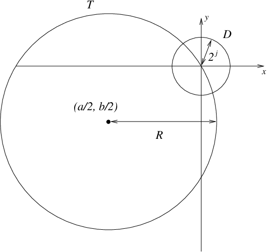
Refer to caption
Figure 2: For RR large enough, the arc T∩DT\cap D contains only 2 lattice points (Case IIA).

Case IIA: If |n|≫|m|\lvert n\rvert\gg\lvert m\rvert and |p|≳23​j\lvert p\rvert\gtrsim 2^{3j}, then there are at most two lattice points on the arc γ:=T∩D\gamma:=T\cap D. The proof follows from Lemma 4.4 in [7] and requires γ\gamma to satisfy:

|γ|≲R1/3.\lvert\gamma\rvert\lesssim R^{1/3}. (7.37)

To see that |p|≳23​j\lvert p\rvert\gtrsim 2^{3j} is sufficient to obtain this bound, we use a small-angle approximation for the left-hand side of (7.37) (the arclength is comparable to the diameter of DD) to get:

|γ|∼2j≲|p|1/3≲|p−m−2​n0|1/3∼R1/3.\begin{split}\lvert\gamma\rvert\sim 2^{j}&\lesssim\lvert p\rvert^{1/3}\\ &\lesssim\lvert p-m-2n_{0}\rvert^{1/3}\\ &\sim R^{1/3}.\end{split} (7.38)

Then we can compute:

∑n,m∈ℤ2|n|≫|m||p|≳23​jδ(∗∗∗)⟨p⟩2⟨p−n−m⟩2​⟨n⟩2​⟨m⟩2≲∑i<j∑|m|∼2i#​Sc⟨n⟩2​⟨m⟩2≲∑j=0∞∑i=0j−1∑|m|∼2i322​j​22​i≲∑j=0∞j22​j<∞.\begin{split}\sum_{\begin{subarray}{c}n,m\in{\mathbb{Z}}^{2}\\ \lvert n\rvert\gg\lvert m\rvert\\ \lvert p\rvert\gtrsim 2^{3j}\end{subarray}}\frac{\delta(***)\langle p\rangle^{2}}{\langle{p-n-m}\rangle^{2}\langle n\rangle^{2}\langle m\rangle^{2}}&\lesssim\sum_{i<j}\sum_{\lvert m\rvert\sim 2^{i}}\frac{\#S_{c}}{\langle n\rangle^{2}\langle m\rangle^{2}}\\ &\lesssim\sum_{j=0}^{\infty}\sum_{i=0}^{j-1}\sum_{\lvert m\rvert\sim 2^{i}}\frac{3}{2^{2j}2^{2i}}\\ &\lesssim\sum_{j=0}^{\infty}\frac{j}{2^{2j}}<\infty.\end{split} (7.39)
Refer to caption
Figure 3: For RR small compared to 2j2^{j}, T∩DT\cap D is the whole circle (Case IIB).

Case IIB: If |n|≫|m|\lvert n\rvert\gg\lvert m\rvert and |p|<23​j\lvert p\rvert<2^{3j}, then because pp is small, the arc γ\gamma is at least a large arc (perhaps the whole circle, as depicted in Figure 3). So we bound the number of lattice points above by the number of lattice points on the whole circle TT, using the Gauss lemma (see also [4]):

#​{ℓ}≤Rε=(|p−m−2​n0|2)ε/2≲((23​j)2)ε/2∼23​j​ε.\begin{split}\#\{\ell\}\leq R^{\varepsilon}&=\left(\lvert p-m-2n_{0}\rvert^{2}\right)^{\varepsilon/2}\\ &\lesssim\left((2^{3j})^{2}\right)^{\varepsilon/2}\\ &\sim 2^{3j\varepsilon}.\end{split} (7.40)

Subcase IIB1: If |p|≫|n|\lvert p\rvert\gg\lvert n\rvert, then we use |p−n−m|∼|p|\lvert p-n-m\rvert\sim\lvert p\rvert for the first step and (7.40) for the second:

∑n,m∈ℤ223​j≳|p|≫|n|≫|m|δ(∗∗∗)⟨p⟩2⟨p−n−m⟩2​⟨n⟩2​⟨m⟩2≲∑i<j∑|m|∼2i#​Sc⟨n⟩2​⟨m⟩2≲∑i<j∑|m|∼2i23​j​ε22​j​22​i≲∑j=0∞∑i=0j−123​j​ε22​j≲∑j=0∞j​23​j​ε22​j.\begin{split}\sum_{\begin{subarray}{c}n,m\in{\mathbb{Z}}^{2}\\ 2^{3j}\gtrsim\lvert p\rvert\gg\lvert n\rvert\gg\lvert m\rvert\end{subarray}}\frac{\delta(***)\langle p\rangle^{2}}{\langle{p-n-m}\rangle^{2}\langle n\rangle^{2}\langle m\rangle^{2}}&\lesssim\sum_{i<j}\sum_{\lvert m\rvert\sim 2^{i}}\frac{\#S_{c}}{\langle{n}\rangle^{2}\langle m\rangle^{2}}\\ &\lesssim\sum_{i<j}\sum_{\lvert m\rvert\sim 2^{i}}\frac{2^{3j\varepsilon}}{2^{2j}2^{2i}}\\ &\lesssim\sum_{j=0}^{\infty}\sum_{i=0}^{j-1}\frac{2^{3j\varepsilon}}{2^{2j}}\\ &\lesssim\sum_{j=0}^{\infty}\frac{j2^{3j\varepsilon}}{2^{2j}}.\end{split} (7.41)

Subcase IIB2: If |p|≲|n|\lvert p\rvert\lesssim\lvert n\rvert, and if |p−n−m|≳|m|\lvert p-n-m\rvert\gtrsim\lvert m\rvert, then we can do a change of variables, z:=p−n−mz:=p-n-m, and we obtain the bound:

∑|n|≫|m||p|≲|n||p−n−m|≳|m|δ(∗∗∗)⟨p⟩2⟨p−n−m⟩2​⟨n⟩2​⟨m⟩2≲∑n∑mδ(∗∗∗)⟨p−m−n⟩2​⟨m⟩2≲∑z∑|m|≲|z|δ⁡(|z|2+|p−m−z|2−|m|2+τ)⟨z⟩2​⟨m⟩2≲∑i<k∑|m|∼2i#​S~c⟨z⟩2​⟨m⟩2,\begin{split}\sum_{\begin{subarray}{c}\lvert n\rvert\gg\lvert m\rvert\\ \lvert p\rvert\lesssim\lvert n\rvert\\ \lvert p-n-m\rvert\gtrsim\lvert m\rvert\end{subarray}}&\frac{\delta(***)\langle p\rangle^{2}}{\langle{p-n-m}\rangle^{2}\langle n\rangle^{2}\langle m\rangle^{2}}\lesssim\sum_{n}\sum_{m}\frac{\delta(***)}{\langle{p-m-n}\rangle^{2}\langle m\rangle^{2}}\\ &\lesssim\sum_{z}\sum_{|m|\lesssim|z|}\frac{\delta(\lvert z\rvert^{2}+\lvert p-m-z\rvert^{2}-\lvert m\rvert^{2}+\tau)}{\langle z\rangle^{2}\langle m\rangle^{2}}\lesssim\sum_{i<k}\sum_{\lvert m\rvert\sim 2^{i}}\frac{\#\tilde{S}_{c}}{\langle{z}\rangle^{2}\langle m\rangle^{2}},\end{split} (7.42)

where

S~c=S~m,k,τ,p:={|z|∼2k:|z|2+|p−m−z|2−|m|2=−τ}.\tilde{S}_{c}=\tilde{S}_{m,k,\tau,p}:=\{\lvert z\rvert\sim 2^{k}:\lvert z\rvert^{2}+\lvert p-m-z\rvert^{2}-\lvert m\rvert^{2}=-\tau\}. (7.43)

By using the same arguments as above we deduce that if |p|>23​k|p|>2^{3k} then we would obtain a bound as in (7.39). On the other hand, in this case, |p|≤23​k|p|\leq 2^{3k}, so we obtain

#​S~c≲2ε​3​k\#\tilde{S}_{c}\lesssim 2^{\varepsilon 3k}

which gives us an estimate similar to the one in (7.39).

Subcase IIB3: If |p|≲|n|\lvert p\rvert\lesssim\lvert n\rvert, and if |p−n−m|≪|m|\lvert p-n-m\rvert\ll\lvert m\rvert, then we can do a change of variables z:=n+mz:=n+m, and proceed:

∑|n|≫|m||p|≲|n||p−n−m|≪|m|δ(∗∗∗)⟨p⟩2⟨p−n−m⟩2​⟨n⟩2​⟨m⟩2≲∑n∑mδ(∗∗∗)⟨p−m−n⟩2​⟨m⟩2≲∑z∑mδ⁡(|p−z|2+|z−m|2−|m|2+τ)⟨p−z⟩2​⟨m⟩2≲∑z∑mδ⁡(|p−z|2+|z−m|2−|m|2+τ)⟨p−z⟩2+ε​⟨m⟩2−ε≲∑z1⟨p−z⟩2+ε​∑mδ⁡(…)⟨m⟩2−ε<∞.\begin{split}\sum_{\begin{subarray}{c}\lvert n\rvert\gg\lvert m\rvert\\ \lvert p\rvert\lesssim\lvert n\rvert\\ \lvert p-n-m\rvert\ll\lvert m\rvert\end{subarray}}&\frac{\delta(***)\langle p\rangle^{2}}{\langle{p-n-m}\rangle^{2}\langle n\rangle^{2}\langle m\rangle^{2}}\lesssim\sum_{n}\sum_{m}\frac{\delta(***)}{\langle{p-m-n}\rangle^{2}\langle m\rangle^{2}}\\ &\lesssim\sum_{z}\sum_{m}\frac{\delta(\lvert p-z\rvert^{2}+\lvert z-m\rvert^{2}-\lvert m\rvert^{2}+\tau)}{\langle p-z\rangle^{2}\langle m\rangle^{2}}\\ &\lesssim\sum_{z}\sum_{m}\frac{\delta(\lvert p-z\rvert^{2}+\lvert z-m\rvert^{2}-\lvert m\rvert^{2}+\tau)}{\langle p-z\rangle^{2+\varepsilon}\langle m\rangle^{2-\varepsilon}}\\ &\lesssim\sum_{z}\frac{1}{\langle p-z\rangle^{2+\varepsilon}}\sum_{m}\frac{\delta(...)}{\langle m\rangle^{2-\varepsilon}}<\infty.\\ \end{split} (7.44)

In the last step, the sum in mm is one-dimensional due to the restraint, and ⟨p−z⟩−ε>⟨m⟩−ε\langle p-z\rangle^{-\varepsilon}>\langle m\rangle^{-\varepsilon} allowed the borrowing to make the two-dimensional sum in zz converge.

Case IIC: |n|∼|m|\lvert n\rvert\sim\lvert m\rvert

Subcase IIC1: If |n|∼|m|≪23​j≲|p|\lvert n\rvert\sim\lvert m\rvert\ll 2^{3j}\lesssim\lvert p\rvert, then we use the fact that |p−n−m|∼|p|\lvert p-n-m\rvert\sim\lvert p\rvert and cancel ⟨p⟩2\langle p\rangle^{2} with ⟨p−n−m⟩2\langle p-n-m\rangle^{2} to estimate like IIA:

∑n,m∈ℤ2|n|∼|m|δ(∗∗∗)⟨p⟩2⟨p−n−m⟩2​⟨n⟩2​⟨m⟩2≲∑i∼j∑|m|∼2i#​Sc⟨n⟩2​⟨m⟩2≲∑i∼j∑|m|∼2i322​i​22​i≲∑i=0∞2−2​i<∞.\begin{split}\sum_{\begin{subarray}{c}n,m\in{\mathbb{Z}}^{2}\\ \lvert n\rvert\sim\lvert m\rvert\end{subarray}}\frac{\delta(***)\langle p\rangle^{2}}{\langle{p-n-m}\rangle^{2}\langle n\rangle^{2}\langle m\rangle^{2}}&\lesssim\sum_{i\sim j}\sum_{\lvert m\rvert\sim 2^{i}}\frac{\#S_{c}}{\langle n\rangle^{2}\langle m\rangle^{2}}\\ &\lesssim\sum_{i\sim j}\sum_{\lvert m\rvert\sim 2^{i}}\frac{3}{2^{2i}2^{2i}}\\ &\lesssim\sum_{i=0}^{\infty}2^{-2i}<\infty.\end{split} (7.45)

Subcase IIC2: If |n|∼|m|≪|p|<23​j\lvert n\rvert\sim\lvert m\rvert\ll\lvert p\rvert<2^{3j}, then we use |p−n−m|∼|p|\lvert p-n-m\rvert\sim\lvert p\rvert for the initial cancellation and use the full-circle bound on the number of lattice points, (7.40), like IIB:

∑n,m∈ℤ2|n|∼|m|δ(∗∗∗)⟨p⟩2⟨p−n−m⟩2​⟨n⟩2​⟨m⟩2≲∑i∼j∑|m|∼2i#​Sc⟨n⟩2​⟨m⟩2≲∑i∼j∑|m|∼2i23​j​ε22​j​22​i≲∑j=0∞23​j​ε22​j.\begin{split}\sum_{\begin{subarray}{c}n,m\in{\mathbb{Z}}^{2}\\ \lvert n\rvert\sim\lvert m\rvert\end{subarray}}\frac{\delta(***)\langle p\rangle^{2}}{\langle{p-n-m}\rangle^{2}\langle n\rangle^{2}\langle m\rangle^{2}}&\lesssim\sum_{i\sim j}\sum_{\lvert m\rvert\sim 2^{i}}\frac{\#S_{c}}{\langle{n}\rangle^{2}\langle m\rangle^{2}}\\ &\lesssim\sum_{i\sim j}\sum_{\lvert m\rvert\sim 2^{i}}\frac{2^{3j\varepsilon}}{2^{2j}2^{2i}}\\ &\lesssim\sum_{j=0}^{\infty}\frac{2^{3j\varepsilon}}{2^{2j}}.\end{split} (7.46)

Subcase IIC3: If |p|≲|n|∼|m|\lvert p\rvert\lesssim\lvert n\rvert\sim\lvert m\rvert, then we cancel ⟨p⟩2\langle p\rangle^{2} with ⟨n⟩2\langle n\rangle^{2} and then use the change of variables z:=n+mz:=n+m in order to bound it:

∑n,m∈ℤ2|n|∼|m|δ(∗∗∗)⟨p⟩2⟨p−n−m⟩2​⟨n⟩2​⟨m⟩2≲∑i∼j∑|m|∼2i∑|n|∼2iδ⁡(τ+|p−n−m|2+|n|2−|m|2)⟨p−n−m⟩2​⟨m⟩2≲∑i∼j∑|m|∼2i∑|z|≲2iδ⁡(τ+|p−z|2+|z−m|2−|m|2)⟨p−z⟩2+ϵ​⟨m⟩2−ε≲∑i=0∞∑|m|∼2i#​S~l⟨m⟩2−ε≲∑i=0∞12i.\begin{split}\sum_{\begin{subarray}{c}n,m\in{\mathbb{Z}}^{2}\\ \lvert n\rvert\sim\lvert m\rvert\end{subarray}}&\frac{\delta(***)\langle p\rangle^{2}}{\langle{p-n-m}\rangle^{2}\langle n\rangle^{2}\langle m\rangle^{2}}\\ &\lesssim\sum_{i\sim j}\sum_{\lvert m\rvert\sim 2^{i}}\sum_{\lvert n\rvert\sim 2^{i}}\frac{\delta(\tau+\lvert p-n-m\rvert^{2}+\lvert n\rvert^{2}-\lvert m\rvert^{2})}{\langle{p-n-m}\rangle^{2}\langle m\rangle^{2}}\\ &\lesssim\sum_{i\sim j}\sum_{\lvert m\rvert\sim 2^{i}}\sum_{\lvert z\rvert\lesssim 2^{i}}\frac{\delta(\tau+\lvert p-z\rvert^{2}+\lvert z-m\rvert^{2}-\lvert m\rvert^{2})}{\langle{p-z}\rangle^{2+\epsilon}\langle m\rangle^{2-\varepsilon}}\\ &\lesssim\sum_{i=0}^{\infty}\sum_{\lvert m\rvert\sim 2^{i}}\frac{\#\tilde{S}_{l}}{\langle m\rangle^{2-\varepsilon}}\lesssim\sum_{i=0}^{\infty}\frac{1}{2^{i}}.\end{split} (7.47)

Here we used the definition, which, we already noticed, defines a line segment:

S~l=Sz,i,τ,p:={|m|∼2i:|p−z|2+|z−m|2−|m|2=−τ},\tilde{S}_{l}=S_{z,i,\tau,p}:=\{\lvert m\rvert\sim 2^{i}:\lvert p-z\rvert^{2}+\lvert z-m\rvert^{2}-\lvert m\rvert^{2}=-\tau\},

This concludes the proof of (7.19), which is the case k=1k=1; the proof for k>1k>1 is similar. ∎

Appendix A Sobolev and Poincaré type inequalities

The following lemma is a simple application of Sobolev inequalities.

Lemma A.1.

For every 1<p≤∞1<p\leq\infty there exists a constant CpC_{p} such that

|⟨ψ,V⁡(x)​ψ⟩|=|∫Λd​x​V​(x)​|ψ⁡(x)|2|≤Cp​‖V‖p​⟨ψ,(1−Δ)​ψ⟩\left|\langle\psi,V(x)\psi\rangle\right|=\left|\int_{\Lambda}{\rm d}x\,V(x)|\psi(x)|^{2}\right|\leq C_{p}\|V\|_{p}\langle\psi,(1-\Delta)\psi\rangle

for every ψ∈L2​(Λ)\psi\in L^{2}(\Lambda). Moreover

|⟨ψ,V⁡(x1−x2)​ψ⟩|≤C​‖V‖1​⟨ψ,(1−Δ1)​(1−Δ2)​ψ⟩\left|\langle\psi,V(x_{1}-x_{2})\psi\rangle\right|\leq C\|V\|_{1}\langle\psi,(1-\Delta_{1})(1-\Delta_{2})\psi\rangle

for all ψ∈Ls2​(Λ×Λ,d​x1​d​x2)\psi\in L^{2}_{s}(\Lambda\times\Lambda,{\rm d}x_{1}{\rm d}x_{2}).

To compare the potential N2​β​V​(Nβ​x)N^{2\beta}V(N^{\beta}x) with the limiting δ\delta-function, we use the following Poincaré type inequality.

Lemma A.2.

Suppose that h∈L1​(Λ)h\in L^{1}(\Lambda) is a probability measure such that ∫Λd​x​(1+x2)1/2​h​(x)<∞\int_{\Lambda}{\rm d}x\,(1+x^{2})^{1/2}\,h(x)<\infty; let hα​(x)=α−2​h​(x/α)h_{\alpha}(x)=\alpha^{-2}h(x/\alpha). Then, for every 0≤κ<10\leq\kappa<1, there exists C>0C>0 such that

|Tr​J(k)​(hα​(xj−xk+1)−δ⁡(xj−xk+1))​γ(k+1)|≤C​ακ​‖|J(k)|‖​Tr​|Sj​Sk+1​γ(k+1)​Sk+1​Sj|\Big|\mbox{Tr}\;J^{(k)}\left(h_{\alpha}(x_{j}-x_{k+1})-\delta(x_{j}-x_{k+1})\right)\gamma^{(k+1)}\Big|\leq C\alpha^{\kappa}\,|\!|\!|J^{(k)}|\!|\!|\,\mbox{Tr}\;\Big|S_{j}S_{k+1}\gamma^{(k+1)}S_{k+1}S_{j}\Big|

for all non-negative γ(k+1)∈ℒk+11\gamma^{(k+1)}\in{\cal L}^{1}_{k+1}.

Proof.

We prove the lemma in the case k=1k=1. For k>1k>1 the proof is analogous. We decompose γ(2)=∑jλj​|φj⟩​⟨φj|\gamma^{(2)}=\sum_{j}\lambda_{j}|\varphi_{j}\rangle\langle\varphi_{j}| for φj∈L2​(Λ2)\varphi_{j}\in L^{2}(\Lambda^{2}), and for eigenvalues λj≥0\lambda_{j}\geq 0. Then we have

Tr​J(1)​(hα​(x1−x2)−δ⁡(x1−x2))​γ(2)=∑jλj​⟨φj,J(1)​(hα​(x1−x2)−δ⁡(x1−x2))​φj⟩=∑jλj​⟨ψj,(hα​(x1−x2)−δ⁡(x1−x2))​φj⟩\begin{split}\mbox{Tr}\,J^{(1)}\left(h_{\alpha}(x_{1}-x_{2})-\delta(x_{1}-x_{2})\right)\gamma^{(2)}=\;&\sum_{j}\lambda_{j}\langle\varphi_{j},J^{(1)}(h_{\alpha}(x_{1}-x_{2})-\delta(x_{1}-x_{2}))\varphi_{j}\rangle\\ =\;&\sum_{j}\lambda_{j}\langle\psi_{j},(h_{\alpha}(x_{1}-x_{2})-\delta(x_{1}-x_{2}))\varphi_{j}\rangle\end{split} (A.1)

where we defined ψj=(J(1)⊗1)​φj\psi_{j}=(J^{(1)}\otimes 1)\varphi_{j}. Next, switching to Fourier space, we observe that

⟨ψj,(hα(x1−x2)−δ(x1−x2))φj⟩=∫d​p1​d​p2​d​q1​d​q2​dx​ψ^¯j​(p1,p2)​φ^j​(q1,q2)​V​(x)​(ei​α​x⋅(p1−q1)−1)​δ​(p1+p2−q1−q2)\begin{split}\langle\psi_{j},&(h_{\alpha}(x_{1}-x_{2})-\delta(x_{1}-x_{2}))\varphi_{j}\rangle\\ &=\int{\rm d}p_{1}{\rm d}p_{2}{\rm d}q_{1}{\rm d}q_{2}{\rm d}x\,\overline{\widehat{\psi}}_{j}(p_{1},p_{2})\widehat{\varphi}_{j}(q_{1},q_{2})\,V(x)\left(e^{i\alpha x\cdot(p_{1}-q_{1})}-1\right)\,\delta(p_{1}+p_{2}-q_{1}-q_{2})\end{split} (A.2)

and thus, taking absolute value, we have, for arbitrary 0<κ<10<\kappa<1,

|⟨ψj,(hα(x1−x2)−δ(x1−x2))φj⟩|≤ακ​(∫d​x​V​(x)​|x|κ)​∫d​p1​d​p2​d​q1​d​q2​|p1−q1|κ​|ψ^j​(p1,p2)|​|φ^j​(q1,q2)|​δ​(p1+p2−q1−q2)\begin{split}\Big|\langle\psi_{j},&(h_{\alpha}(x_{1}-x_{2})-\delta(x_{1}-x_{2}))\varphi_{j}\rangle\Big|\\ &\leq\alpha^{\kappa}\,\left(\int{\rm d}x\,V(x)|x|^{\kappa}\right)\int{\rm d}p_{1}{\rm d}p_{2}{\rm d}q_{1}{\rm d}q_{2}\,|p_{1}-q_{1}|^{\kappa}|\widehat{\psi}_{j}(p_{1},p_{2})||\widehat{\varphi}_{j}(q_{1},q_{2})|\delta(p_{1}+p_{2}-q_{1}-q_{2})\end{split} (A.3)

Estimating |p1−q1|κ≤|p1|κ+|q1|κ|p_{1}-q_{1}|^{\kappa}\leq|p_{1}|^{\kappa}+|q_{1}|^{\kappa} we have to control two terms. We show how to control the term containing |p1|κ|p_{1}|^{\kappa} (the term with |q1|κ|q_{1}|^{\kappa} can be bounded similarly):

∫d​p1​d​p2​d​q1d​q2​|p1|κ​|ψ^j​(p1,p2)|​|φ^j​(q1,q2)|​δ​(p1+p2−q1−q2)≤∫d​p1​d​p2​d​q1​d​q2​δ​(p1+p2−q1−q2)×(1+p12)1/2​(1+p22)1/2(1+q22)1/2​(1+q12)1/2​|ψ^j​(p1,p2)|​(1+q22)1/2​(1+q12)1/2(1+p12)(1−κ)/2​(1+p22)1/2​|φ^j​(q1,q2)|≤δ​∫d​p1​d​p2​d​q1​d​q2​(1+p12)​(1+p22)(1+q22)​(1+q12)​|ψ^j​(p1,p2)|2​δ​(p1+p2−q1−q2)+δ−1∫dp1dp2dq1dq2(1+q22)​(1+q12)(1+p12)(1−κ)​(1+p22)|φ^j(q1,q2)|2δ(p1+p2−q1−q2)≤δ⁡⟨ψj,S12​S22​ψj⟩​supp∈Λ∫d​q​1(1+(p−q)2)​(1+q2)+δ−1⟨φj,S12S22φj⟩supq∈Λ∫dp1(1+(q−p)2)(1−κ)​(1+p2)\begin{split}\int{\rm d}p_{1}{\rm d}p_{2}{\rm d}q_{1}&{\rm d}q_{2}\,|p_{1}|^{\kappa}|\widehat{\psi}_{j}(p_{1},p_{2})||\widehat{\varphi}_{j}(q_{1},q_{2})|\delta(p_{1}+p_{2}-q_{1}-q_{2})\\ \leq\;&\int{\rm d}p_{1}{\rm d}p_{2}{\rm d}q_{1}{\rm d}q_{2}\,\delta(p_{1}+p_{2}-q_{1}-q_{2})\\ &\hskip 14.22636pt\times\frac{(1+p^{2}_{1})^{1/2}(1+p^{2}_{2})^{1/2}}{(1+q_{2}^{2})^{1/2}(1+q_{1}^{2})^{1/2}}\,|\widehat{\psi}_{j}(p_{1},p_{2})|\frac{(1+q_{2}^{2})^{1/2}(1+q_{1}^{2})^{1/2}}{(1+p^{2}_{1})^{(1-\kappa)/2}(1+p^{2}_{2})^{1/2}}|\widehat{\varphi}_{j}(q_{1},q_{2})|\\ \leq\;&\delta\int{\rm d}p_{1}{\rm d}p_{2}{\rm d}q_{1}{\rm d}q_{2}\,\frac{(1+p^{2}_{1})(1+p^{2}_{2})}{(1+q_{2}^{2})(1+q_{1}^{2})}\,|\widehat{\psi}_{j}(p_{1},p_{2})|^{2}\delta(p_{1}+p_{2}-q_{1}-q_{2})\\ &+\delta^{-1}\int{\rm d}p_{1}{\rm d}p_{2}{\rm d}q_{1}{\rm d}q_{2}\,\frac{(1+q_{2}^{2})(1+q_{1}^{2})}{(1+p^{2}_{1})^{(1-\kappa)}(1+p^{2}_{2})}|\widehat{\varphi}_{j}(q_{1},q_{2})|^{2}\delta(p_{1}+p_{2}-q_{1}-q_{2})\\ \leq\;&\delta\,\langle\psi_{j},S_{1}^{2}S_{2}^{2}\psi_{j}\rangle\sup_{p\in\Lambda}\int{\rm d}q\,\frac{1}{(1+(p-q)^{2})(1+q^{2})}\\ &+\delta^{-1}\,\langle\varphi_{j},S_{1}^{2}S_{2}^{2}\varphi_{j}\rangle\sup_{q\in\Lambda}\int{\rm d}p\,\frac{1}{(1+(q-p)^{2})^{(1-\kappa)}(1+p^{2})}\end{split} (A.4)

for arbitrary δ>0\delta>0. Since

supq∈Λ∫d​p​1(1+(q−p)2)(1−κ)​(1+p2)<∞\sup_{q\in\Lambda}\int{\rm d}p\,\frac{1}{(1+(q-p)^{2})^{(1-\kappa)}(1+p^{2})}<\infty

for all 0≤κ<10\leq\kappa<1, from (A.1) and (A.3) we obtain that

|TrJ(1)(hα(x1−x2)−δ(x1−x2))γ(2)|≤C​ακ​(δ​Tr​J(1)​S12​S22​J(1)​γ(2)+δ−1​Tr​S12​S22​γ(2))≤C​ακ​(δ​Tr​S1−1​J(1)​S12​J(1)​S1−1​S1​S2​γ(2)​S2​S1+δ−1​Tr​S12​S22​γ(2))≤C​ακ​(δ​‖S1−1​J(1)​S1‖​‖S1​J(1)​S1−1‖+δ−1)​Tr​S12​S22​γ(2)≤C​ακ​‖|J(1)|‖​Tr​S12​S22​γ(2)\begin{split}\Big|\mbox{Tr}\,J^{(1)}\Big(h_{\alpha}(x_{1}-x_{2})-&\delta(x_{1}-x_{2})\Big)\gamma^{(2)}\Big|\\ \leq\;&C\alpha^{\kappa}\left(\delta\,\mbox{Tr}\,J^{(1)}S_{1}^{2}S_{2}^{2}J^{(1)}\gamma^{(2)}+\delta^{-1}\,\mbox{Tr}\,S_{1}^{2}S_{2}^{2}\gamma^{(2)}\right)\\ \leq\;&C\alpha^{\kappa}\left(\delta\,\mbox{Tr}\,S_{1}^{-1}J^{(1)}S_{1}^{2}J^{(1)}S_{1}^{-1}S_{1}S_{2}\gamma^{(2)}S_{2}S_{1}+\delta^{-1}\,\mbox{Tr}\,S_{1}^{2}S_{2}^{2}\gamma^{(2)}\right)\\ \leq\;&C\alpha^{\kappa}\left(\delta\,\|S_{1}^{-1}J^{(1)}S_{1}\|\,\|S_{1}J^{(1)}S_{1}^{-1}\|+\delta^{-1}\right)\mbox{Tr}S_{1}^{2}S_{2}^{2}\gamma^{(2)}\\ \leq\;&C\alpha^{\kappa}|\!|\!|J^{(1)}|\!|\!|\,\mbox{Tr}S_{1}^{2}S_{2}^{2}\gamma^{(2)}\end{split} (A.5)

where, in the last inequality we chose δ=‖|J(1)|‖−1\delta=|\!|\!|J^{(1)}|\!|\!|^{-1}. ∎

Acknowledgements

K. Kirkpatrick (kay@math.mit.edu) is supported by NSF postdoctoral research fellowship DMS-0703618. B. Schlein (schlein@math.lmu.de) is on leave from Cambridge University; his research is supported by a Sofja Kovalevskaya Award of the Alexander von Humboldt Foundation. G. Staffilani (gigliola@math.mit.edu) is partially supported by NSF grant DMS-0602678.

References

  • [1] R. Adami, C. Bardos, F. Golse, and A. Teta, Towards a rigorous derivation of the cubic nonlinear Schrödinger equation in dimension one. Asymptot. Anal. 40 (2004), no. 2, 93–108.
  • [2] R. Adami, F. Golse, and A. Teta, Rigorous derivation of the cubic NLS in dimension one. J. Stat. Phys. 127 (2007), no. 6, 1193–1220.
  • [3] C. Bardos, F. Golse, and N. Mauser, Weak coupling limit of the NN-particle Schrödinger equation. Methods Appl. Anal. 7 (2000), 275–293.
  • [4] E. Bombieri and J. Pila, The number of integral points on arcs and ovals, Duke Math. J. 59 (1989), no. 2, 337–357.
  • [5] J. Bourgain, Fourier transform restriction phenomena for certain lattice subsets and applications to nonlinear evolution equations I-II, Geom. Funct. Anal., 3 (1993), 107–156, 209–262.
  • [6] J. Bourgain, On Strichartz inequalities and the nonlinear Schrodinger equation on irrational tori, preprint.
  • [7] D. De Silva, N. Pavlović, G. Staffilani, and N. Tzirakis, Global well-posedness for a periodic nonlinear Schrödinger equation in 1D and 2D, arXiv: math.AP/0602660v1 (2006).
  • [8] A. Elgart, L. Erdős, B. Schlein, and H.-T. Yau, Gross-Pitaevskii equation as the mean field limit of weakly coupled bosons. Arch. Rat. Mech. Anal. 179 (2006), no. 2, 265–283.
  • [9] A. Elgart and B. Schlein, Mean Field Dynamics of Boson Stars. Commun. Pure Appl. Math. 60 (2007), no. 4, 500–545.
  • [10] L. Erdős, B. Schlein, and H.-T. Yau, Derivation of the cubic non-linear Schrödinger equation from quantum dynamics of many-body systems. Invent. Math. 167 (2007), 515–614.
  • [11] L. Erdős, B. Schlein, and H.-T. Yau, Derivation of the Gross-Pitaevskii Equation for the Dynamics of Bose-Einstein Condensate. Preprint arXiv:math-ph/0606017. To appear in Ann. Math.
  • [12] L. Erdős, B. Schlein, and H.-T. Yau, Rigorous Derivation of the Gross-Pitaevskii Equation with a Large Interaction Potential. Preprint arXiv:0802.3877.
  • [13] L. Erdős and H.-T. Yau, Derivation of the nonlinear Schrödinger equation from a many body Coulomb system. Adv. Theor. Math. Phys. 5 (2001), no. 6, 1169–1205.
  • [14] E. Gross, Structure of a quantized vortex in boson systems. Nuovo Cimento 20 (1961), 454–466.
  • [15] J. Ginibre and G. Velo, The classical field limit of scattering theory for nonrelativistic many-boson systems. I.-II. Comm. Math. Phys. 66 (1979), no. 1, 37–76, and 68 (1979), no. 1, 45–68.
  • [16] J. Ginibre and G. Velo, On a class of nonlinear Schrödinger equations with nonlocal interactions. Math Z. 170 (1980), 109-136.
  • [17] J. Ginibre and G. Velo, Scattering theory in the energy space for a class of nonlinear Schrödinger equations. J. Math. Pures Appl. 64 (1985), 363-401.
  • [18] K. Hepp, The classical limit for quantum mechanical correlation functions. Comm. Math. Phys. 35 (1974), 265–277.
  • [19] M. N. Huxley, Area, Lattice Points, and Exponential Sums. London Mathematical Society Monographs, 13 (1996).
  • [20] K. Ireland and M. Rosen, A Classical Introduction to Modern Number Theory, 2nd edition. Graduate Texts in Mathematics, 84. Springer-Verlag, New York (1998).
  • [21] S. Klainerman and M. Machedon, On the uniqueness of solutions to the Gross-Pitaevskii hierarchy. Comm. Math. Phys. 279 (2008), no. 1, 169–185.
  • [22] E. H. Lieb and R. Seiringer, Proof of Bose-Einstein condensation for dilute trapped gases. Phys. Rev. Lett. 88 (2002), 170409-1-4.
  • [23] E. H. Lieb, R. Seiringer, and J. Yngvason, A rigorous derivation of the Gross-Pitaevskii energy functional for a two-dimensional Bose gas. Comm. Math. Phys. 224 (2001), 17–31.
  • [24] E. H. Lieb, R. Seiringer, and J. Yngvason, Bosons in a trap: A rigorous derivation of the Gross-Pitaevskii energy functional. Phys. Rev A 61 (2000), 043602.
  • [25] L. Pitaevskii, Vortex lines in an imperfect Bose gas. Sov. Phys. JETP 13 (1961), 451–454.
  • [26] M. Reed and B. Simon, Methods of modern mathematical physics: Scattering Theory. Volume 3. Academic Press, 1979.
  • [27] I. Rodnianski and B. Schlein, Quantum fluctuations and rate of convergence towards mean field dynamics. Preprint arXiv:math-ph/0711.3087.
  • [28] W. Rudin, Functional analysis. McGraw-Hill Series in Higher Mathematics, McGraw-Hill Book Co., New York, 1973.
  • [29] H. Spohn, Kinetic Equations from Hamiltonian Dynamics. Rev. Mod. Phys. 52 (1980), no. 3, 569–615.