跳到论文正文
W Papers独立论文阅读器 arXiv:0808.0228 论文正文 计算阅读时间 · 0%
引用这篇论文根据当前论文元数据生成,正式投稿前建议核对。


License: arXiv.org perpetual non-exclusive license
arXiv:0808.0228v1 [math.AP] 02 Aug 2008

Non-variational computation
of the eigenstates of Dirac operators
with radially symmetric potentials

Lyonell Boulton Address: Department of Mathematics and Maxwell Institute for Mathematical Sciences, Heriot-Watt University, Edinburgh EH14 4AS, United Kingdom Email address: L.Boulton@hw.ac.uk and Nabile Boussaid Address: Département de Mathématiques, UFR Sciences et techniques - 16, route de Gray - 25 030, Besançon cedex, France Email address: nabile.boussaid@univ-fcomte.fr
Date: July 2008
Abstract.

We discuss a novel strategy for computing the eigenvalues and eigenfunctions of the relativistic Dirac operator with a radially symmetric potential. The virtues of this strategy lie on the fact that it avoids completely the phenomenon of spectral pollution and it always provides two-side estimates for the eigenvalues with explicit error bounds on both eigenvalues and eigenfunctions. We also discuss convergence rates of the method as well as illustrate our results with various numerical experiments.

Key words and phrases: 
Dirac operators, quadratic projection methods, spectral pollution

1. Introduction

The free Dirac operator acting on 4-spinors of L2​(ℝ3)4L^{2}(\mathbb{R}^{3})^{4} is determined by the first order differential expression

D:=α⋅P+β=−i∑k=13αk∂k+β,D:=\alpha\cdot P+\beta=-{\rm i}\sum_{k=1}^{3}\alpha_{k}\partial_{k}+\beta,

where α=(α1,α2,α3)\alpha=\left(\alpha_{1},\alpha_{2},\alpha_{3}\right), and the Pauli-Dirac matrices are:

αi=(0σiσi0) and β=(Iℂ200−Iℂ2),\displaystyle\alpha_{i}=\left(\begin{array}[]{cc}0&\sigma_{i}\\ \sigma_{i}&0\end{array}\right)\quad\mbox{ and }\quad\beta=\left(\begin{array}[]{cc}I_{\mathbb{C}^{2}}&0\\ 0&-I_{\mathbb{C}^{2}}\end{array}\right),
 for ​σ1=(0 11 0),σ2=(0−ii0) and ,σ3=(100−1).\displaystyle\mbox{ for }\sigma_{1}=\left(\begin{array}[]{cc}0&\;1\\ 1&\;0\end{array}\right),\quad\quad\sigma_{2}=\left(\begin{array}[]{cc}0&-{\rm i}\\ {\rm i}&0\end{array}\right)\quad\mbox{ and }\quad\sigma_{3}=\left(\begin{array}[]{cc}1&0\\ 0&-1\end{array}\right).

We assume that the units are fixed so that m=c=ℏ=1m=c=\hbar=1. Standard arguments involving the Fourier transform show that DD defines a self-adjoint operator with domain H1​(ℝ3)4H^{1}(\mathbb{R}^{3})^{4} and that the spectrum of DD is

Spec(D)=(−∞,−1]∪[1,∞).\operatorname{Spec}(D)=(-\infty,-1]\cup[1,\infty).

Spherically symmetric potentials are Hermitean 4×44\times 4 matrix multiplication operators, VV, acting on L2​(ℝ2)4L^{2}(\mathbb{R}^{2})^{4}, such that 𝒞0∞​(ℝ3∖{0})⊂Dom⁡(V){\mathcal{C}}^{\infty}_{0}(\mathbb{R}^{3}\setminus\{0\})\subset\operatorname{Dom}(V) and

ei​φ​n⋅SV(R−1x)e−iφn⋅S=V(x),∀x∈ℝ3,∀φ∈[0,4π),e^{{\rm i}\varphi n\cdot S}V(R^{-1}x)e^{-{\rm i}\varphi n\cdot S}=V(x),\;\forall x\in\mathbb{R}^{3},\;\forall\varphi\in[0,4\pi),

where

S=12​(0σσ0)S=\frac{1}{2}\begin{pmatrix}0&\sigma\\ \sigma&0\end{pmatrix}

is the spin operator, and RR is the matrix of the rotation of angle φ\varphi and axis nn. Here Dom⁡(V)\operatorname{Dom}(V) denotes the maximal domain of VV.

Spherically symmetric potentials may be constructed from maps ϕsc,el,am:ℝ⟶ℝ\phi_{\mathrm{sc},\mathrm{el},\mathrm{am}}:\mathbb{R}\longrightarrow\mathbb{R} via

(1.1) V⁡(x)=ϕsc​(|x|)​β+ϕel​(|x|)​Iℂ4+i​ϕam​(|x|)​β​α⋅x|x|.V(x)=\phi_{\mathrm{sc}}(|x|)\beta+\phi_{\mathrm{el}}(|x|)I_{\mathbb{C}^{4}}+i\phi_{\mathrm{am}}(|x|)\beta\alpha\cdot\frac{x}{|x|}.

The subscripts “sc\mathrm{sc}”, “el\mathrm{el}” and “am\mathrm{am}”, stand for “scalar”, “electric” and “magnetic” potential, respectively. Radial symmetry on the electric potential, for instance, is a consequence of the assumption that the atomic nucleus is pointwise and the electric forces are isotropic in an isotropic medium like the vacuum. In the particular case ϕsc=ϕam=0\phi_{\mathrm{sc}}=\phi_{\mathrm{am}}=0 and ϕel​(r)=γ/r\phi_{\mathrm{el}}(r)=\gamma/r, |γ|<3/2|\gamma|<\sqrt{3}/2, HH describes the motion of a relativistic electron in the field created by an atomic nucleus.

If VV is subject to suitable smallness and regularity conditions (such as those ensuring that VV is relatively compact with respect to DD), then H:=D+VH:=D+V defines an essentially self-adjoint operator in C0∞​(ℝ3∖{0})4C^{\infty}_{0}(\mathbb{R}^{3}\setminus\{0\})^{4} with self-adjoint extension domain H1​(ℝ3)4H^{1}(\mathbb{R}^{3})^{4} and

(1.2) Specess(H)=Spec(D)=(−∞,−1]∪[1,∞),\operatorname{Spec}_{\text{ess}}(H)=\operatorname{Spec}(D)=(-\infty,-1]\cup[1,\infty),

see [Tha92, Theorems 4.2 and 4.16]. In fact there are known conditions, satisfied by potentials of practical interest (see e.g. [BG87, Theorems 6 and A]), preventing the existence of embedded eigenvalues.

The addition of a non-zero potential might give rise to a non-empty discrete spectrum in the gap (−1,1)(-1,1). These eigenvalues can only be found explicitly for a few simple systems which do not go much beyond the case of a single electron embedded in a field created by an atomic nucleus, see (4.1). For more complicated potentials, one has to rely either on asymptotic techniques (cf. [BL94], [GL99], [Sch03] and references therein) or on numerical estimations.

Few robust computational procedures are currently available to estimate numerically the eigenvalues of HH, see [Dya90], [DES00], [DESV00], [DES03], [DEL07], [LLT02] and references therein. Since HH is strongly indefinite, a direct implementation of the projection method is not possible due to variational collapse. Under no further restriction on the potential or the reduction basis, accumulation points of eigenvalues of the finite dimensional approximate operator which do not belong to Spec⁡(H)\operatorname{Spec}(H) might appear, see [SH84] and [Dya90]. This phenomenon is known as spectral pollution.

The aim of the present paper is to investigate the applicability of the so called quadratic projection method for finding eigenvalues and eigenfunctions of HH. This method has been recently studied in an abstract setting (see [Sha00], [LS04], [Bou06] and [Bou07]) and it has already been applied with some success to crystalline Schrödinger operators, [BL07], and magnetohydrodynamics, [Str08]. In this approach, explained at length in Section 3, the underlying discretised eigenvalue problem is quadratic in the spectral parameter (rather than linear), and has non-real eigenvalues. Its main advantage over a standard projection method is its robustness: it never pollutes and it always provides a posteriori two-sided estimates of the error of computed eigenvalues.

Section 3.1 is devoted to a self-contained description of the quadratic projection method. In Theorem 1 we present an alternative proof of Shargorodsky’s non-pollution Theorem [LS04, Theorem 2.6]. Additionally we show that information about eigenfunctions can be recovered from the quadratic projection method, see (3.4).

In Section 4 we test the practical applicability of the numerical scheme proposed in Section 3 by reporting on various numerical experiments. As benchmark potentials we have chosen the purely coulombic, sub-coulombic and inverse harmonic electric potentials. In order to perform these numerical experiments, we split the space into upper and lower spinor component, after writing the problem in radial form. Spectral pollution in the standard projection method using this decomposition and the consequences of unbalancing the number of upper/lower components is discussed in Section 2.

We have chosen a basis of Hermite functions to reduce the continuous problem into finite-dimensional from. In Section 3.3 we perform a rigourous convergence analysis of the quadratic method using this basis. This analysis relies upon the general result [Bou07, Theorem 2.1]. The surprising numerical evidence included in Section 4.4 strongly suggest that, under appropriate circumstances, choosing a basis that heavily pollute the standard projection method, significantly improves convergence rates of the quadratic projection method.

We have posted a fully functional Matlab code for assembling the matrices involved in the quadratic projection method for VV a coulombic potential in the Manchester NLEVP collection of non-linear eigenvalue problems [BHM+08]. See the permanent link [BHM+]. In Appendix A we include details of the explicit calculation of all matrix coefficients.

2. Spectral pollution and upper/lower spinor component balance

Consider, for any Ψ∈L2​(ℝ3)4\Psi\in L^{2}(\mathbb{R}^{3})^{4}, the spherical coordinates representation:

(2.1) ψ⁡(r,θ,ϕ)=r​Ψ​(r​sin⁡(θ)​sin⁡(ϕ),r​sin⁡(θ)​cos⁡(ϕ),r​cos⁡(θ))\psi(r,\theta,\phi)=r\Psi(r\sin(\theta)\sin(\phi),r\sin(\theta)\cos(\phi),r\cos(\theta))

where (r,θ,ϕ)∈(0,∞)×[0,π)×[−π,π)(r,\theta,\phi)\in(0,\infty)\times[0,\pi)\times[-\pi,\pi). The map Ψ↦ψ\Psi\mapsto\psi is an isomorphism between L2​(ℝ3)4L^{2}(\mathbb{R}^{3})^{4} and L2​((0,∞),d​r)⊗L2​(S2)4L^{2}((0,\infty),dr)\otimes L^{2}(S^{2})^{4}. If we decompose L2​(S2)4L^{2}(S^{2})^{4} as the sum of the so called two-dimensional angular momentum subspaces 𝔎mj,κj{\mathfrak{K}}_{m_{j},\kappa_{j}}, the partial wave subspaces are given by

ℌmj,κj=L2​((0,∞),d​r)⊗𝔎mj,κj,{\mathfrak{H}}_{m_{j},\kappa_{j}}=L^{2}((0,\infty),dr)\otimes{\mathfrak{K}}_{m_{j},\kappa_{j}},

so that L2​(ℝ3)4=⨁ℌmj,κjL^{2}(\mathbb{R}^{3})^{4}=\bigoplus{\mathfrak{H}}_{m_{j},\kappa_{j}}. Without further mention, here and below we always assume that the indices (mj,κj)(m_{j},\kappa_{j}) run over the set mj∈{−j,⋯,j}m_{j}\in\{-j,\cdots,j\} and κj∈{±(j+12)}\kappa_{j}\in\{\pm(j+\frac{1}{2})\}, for j∈{2​k+12:k∈ℕ}j\in\{\frac{2k+1}{2}:k\in\mathbb{N}\}.

The rr factor in (2.1) renders a Dirichlet boundary condition at 00. The dense subspaces C0∞​(0,∞)⊗𝔎mj,κj⊂ℌmj,κjC^{\infty}_{0}(0,\infty)\otimes{\mathfrak{K}}_{m_{j},\kappa_{j}}\subset{\mathfrak{H}}_{m_{j},\kappa_{j}} are invariant under the action of HH. If VV is as in (1.1), then H↾C0∞​(0,∞)⊗𝔎mj,κjH\upharpoonright C^{\infty}_{0}(0,\infty)\otimes{\mathfrak{K}}_{m_{j},\kappa_{j}} is unitary equivalent to

(2.2) Hmj,κj:=(1+ϕsc​(r)+ϕel​(r)−dd​r+κjr+ϕam​(r)dd​r+κjr+ϕam​(r)−1−ϕsc​(r)+ϕel​(r)).H_{m_{j},\kappa_{j}}:=\begin{pmatrix}1+\phi_{\mathrm{sc}}(r)+\phi_{\mathrm{el}}(r)&-\frac{d}{dr}+\frac{\kappa_{j}}{r}+\phi_{\mathrm{am}}(r)\\ \frac{d}{dr}+\frac{\kappa_{j}}{r}+\phi_{\mathrm{am}}(r)&-1-\phi_{\mathrm{sc}}(r)+\phi_{\mathrm{el}}(r)\end{pmatrix}.

The operators Hmj,κjH_{m_{j},\kappa_{j}} are essentially self-adjoint in C0∞​(0,∞)2C^{\infty}_{0}(0,\infty)^{2} under suitable conditions on the potentials ϕsc,el,am\phi_{\mathrm{sc},\mathrm{el},\mathrm{am}}. Then

Spec⁡(H)=⋃Spec⁡(Hmj,κj)¯.\operatorname{Spec}(H)=\overline{\bigcup\operatorname{Spec}(H_{m_{j},\kappa_{j}})}.

Below we often suppress the sub-index (mj,κj)(m_{j},\kappa_{j}) from operators and spaces, and only write the index κ≡κj\kappa\equiv\kappa_{j}. Note that the eigenvalues of HH are degenerate and their multiplicity is at least mjm_{j}. By virtue of (1.2),

Specdisc⁡(H)=⋃Specdisc⁡(Hκ).\operatorname{Spec}_{\text{disc}}(H)=\bigcup\operatorname{Spec}_{\text{disc}}(H_{\kappa}).

Since Specess(Hκ)=(−∞,−1]∪[1,∞)\operatorname{Spec}_{\text{ess}}(H_{\kappa})=(-\infty,-1]\cup[1,\infty), HκH_{\kappa} are strongly indefinite.

Let us consider a heuristic approach to the problem of spectral pollution for HκH_{\kappa} and the decomposition of L2​(0,∞)2L^{2}(0,\infty)^{2} into upper and lower spinor components. For simplicity we assume that the potential is purely electric and attractive, ϕsc​(r)=ϕam​(r)=0\phi_{\mathrm{sc}}(r)=\phi_{\mathrm{am}}(r)=0 and ϕel​(r)<0\phi_{\mathrm{el}}(r)<0.

The pair (u,v)∈Dom⁡(Hκ)(u,v)\in\operatorname{Dom}(H_{\kappa}) is a wave function of HκH_{\kappa} with associated eigenvalue E∈(−1,1)E\in(-1,1) if and only if

(2.3) (ϕel+1−E)u+(−∂r+κr)v=0and(∂r+κr)u+(ϕel−1−E)v=0.(\phi_{\mathrm{el}}+1-E)u+(-\partial_{r}+\frac{\kappa}{r})v=0\qquad\text{and}\qquad(\partial_{r}+\frac{\kappa}{r})u+(\phi_{\mathrm{el}}-1-E)v=0.

System (2.3) can be decoupled into

(2.4) LEu=0andv=−(ϕel−1−E)−1(∂r+κr)u,\qquad L_{E}u=0\qquad\text{and}\qquad v=-(\phi_{\mathrm{el}}-1-E)^{-1}\left(\partial_{r}+\frac{\kappa}{r}\right)u,

where

LE\displaystyle L_{E} :=−(−∂r+κr)(ϕel−1−E)−1(∂r+κr)+(ϕel+1−E)\displaystyle:=-\left(-\partial_{r}+\frac{\kappa}{r}\right)(\phi_{\mathrm{el}}-1-E)^{-1}\left(\partial_{r}+\frac{\kappa}{r}\right)+(\phi_{\mathrm{el}}+1-E)
≥(1+E)−1(∂r+κr)∗(∂r+κr)+ϕel+(1−E).\displaystyle\geq(1+E)^{-1}\left(\partial_{r}+\frac{\kappa}{r}\right)^{\ast}\left(\partial_{r}+\frac{\kappa}{r}\right)+\phi_{\mathrm{el}}+(1-E).

If we assume ϕel\phi_{\mathrm{el}} is relatively compact with respect to the non-negative operator (∂r+κr)∗(∂r+κr)(\partial_{r}+\frac{\kappa}{r})^{\ast}(\partial_{r}+\frac{\kappa}{r}),

(2.5) min⁡Specess⁡LE≥(1−E)>0.\min\operatorname{Spec}_{\text{ess}}L_{E}\geq(1-E)>0.

Moreover, the expression for vv in (2.4) yields u≢0u\not\equiv 0 and v≢0v\not\equiv 0. Hence E∈Specdisc⁡HκE\in\operatorname{Spec}_{\text{disc}}H_{\kappa} if and only if 00 is in the discrete spectrum of LEL_{E}.

Let ℳN⊂L2​(0,∞)\mathcal{M}_{N}\subset L^{2}(0,\infty) be a nested family of finite-dimensional subspaces such that ℳN⊂ℳN+1\mathcal{M}_{N}\subset\mathcal{M}_{N+1},

⋃N≥1ℳN¯=L2​(0,∞)\overline{\bigcup_{N\geq 1}\mathcal{M}_{N}}=L^{2}(0,\infty)

and ℒN​M:=ℳN⊕ℳM⊂Dom⁡(Hκ)\mathcal{L}_{NM}:=\mathcal{M}_{N}\oplus\mathcal{M}_{M}\subset\operatorname{Dom}(H_{\kappa}). Let PNP_{N} denote the orthogonal projection onto ℳN\mathcal{M}_{N}, so that PN→IP_{N}\to I in the strong sense. With this notation we wish to apply the projection method to operator HκH_{\kappa} with test spaces ℒN​M\mathcal{L}_{NM}.

We first consider the case N=MN=M. Let (uN,vN)t∈ℒN​N(u_{N},v_{N})^{t}\in\mathcal{L}_{NN} be a sequence normalised by ‖uN‖2+‖vN‖2=1\|u_{N}\|^{2}+\|v_{N}\|^{2}=1, such that

(2.6) PN[(ϕel+1−EN)uN+(−∂r+κr)vN]=0,\displaystyle P_{N}[(\phi_{\mathrm{el}}+1-E_{N})u_{N}+(-\partial_{r}+\frac{\kappa}{r})v_{N}]=0,
(2.7) PN[(∂r+κr)uN+(ϕel−1−EN)vN]=0\displaystyle P_{N}[(\partial_{r}+\frac{\kappa}{r})u_{N}+(\phi_{\mathrm{el}}-1-E_{N})v_{N}]=0

for a suitable sequence EN→E~∈(−1,1)E_{N}\to\tilde{E}\in(-1,1). Let χN\chi_{N} be such that

vN=−(ϕel−1−EN)−1(∂r+κr)uN+χN.v_{N}=-(\phi_{\mathrm{el}}-1-E_{N})^{-1}\left(\partial_{r}+\frac{\kappa}{r}\right)u_{N}+\chi_{N}.

By virtue of (2.7),

(2.8) PN​(ϕel−1−EN)​χN=0.P_{N}(\phi_{\mathrm{el}}-1-E_{N})\chi_{N}=0.

If we where able to prove that

(2.9) ∥PN(−∂r+κr)χN∥→0,N→∞,\|P_{N}(-\partial_{r}+\frac{\kappa}{r})\chi_{N}\|\to 0,\qquad N\to\infty,

by substituting into (2.6), we would have ‖PN​LE~​uN‖→0\|P_{N}L_{\tilde{E}}u_{N}\|\to 0. Thus, by virtue of the min-max principle alongside with (2.5), we would have 0∈Specdisc⁡LE~0\in\operatorname{Spec}_{\text{disc}}L_{\tilde{E}} and so E~∈Specdisc⁡Hκ\tilde{E}\in\operatorname{Spec}_{\text{disc}}H_{\kappa}.

Unfortunately, (2.9) can not be easily verified. Since PN→IP_{N}\to I in the strong sense, (ϕel−1−EN)​χN→0(\phi_{\mathrm{el}}-1-E_{N})\chi_{N}\to 0 in the weak sense. Since ϕel<0\phi_{\mathrm{el}}<0, χN→0\chi_{N}\to 0 also in the weak sense. Therefore we are certain that (−∂r+κr)χN→0(-\partial_{r}+\frac{\kappa}{r})\chi_{N}\to 0 and hence PN​LE~​uN→0P_{N}L_{\tilde{E}}u_{N}\to 0 weakly. This does not imply in general (2.9), it only gives indication that the latter is a sensible guess.

The key idea behind the above heuristic argument motivates several pollution-free numerical methods for computing eigenvalues of HκH_{\kappa}, including the quadratic projection method discussed in the forthcoming section: as (2.3) might be vulnerable to spectral pollution in the gap (−1,1)(-1,1) because (2.9) is not necessarily guaranteed, we characterise the eigenvalues of this problem by testing whether 00 is in the spectrum of an auxiliary operator. This auxiliary operator has essential spectrum in {Re(z)>0}\{\operatorname{Re}(z)>0\}, so that a neighbourhood of 00 is always protected against spectral pollution (see the discussion preceding [Bou06, Lemma 5].) In the quadratic projection method, (2.9) is substituted by (3.4).

Remark 1.

A successful procedure for computing eigenvalues of the Dirac operator is the one developed by Dolbeault, Esteban and Séré, [DES00] and [DES03]. This procedure systematically implements the above idea. Multiplying by uu the left side equation of (2.4) and integrating in the space variable, gives A⁡(E)​u=0A(E)u=0 for

A⁡(λ)​v:=∫0∞|(rκ​v)′|2r2​κ​(1+λ−ϕel)+(ϕel+1−λ)​|v|2​𝑑r.A(\lambda)v:=\int_{0}^{\infty}\frac{|(r^{\kappa}v)^{\prime}|^{2}}{r^{2\kappa}(1+\lambda-\phi_{\mathrm{el}})}+(\phi_{\mathrm{el}}+1-\lambda)|v|^{2}\,\mathrm{d}r.

Both terms inside the integral decrease in λ\lambda so, if vv is regular enough, there is a unique λ=λ⁡(v)∈ℝ\lambda=\lambda(v)\in\mathbb{R} satisfying A⁡(λ)​v=0A(\lambda)v=0. Upper estimates for the eigenvalues of HκH_{\kappa} are then found from those of the matrix corresponding to the λ\lambda-dependant form A⁡(λ)​vA(\lambda)v restricted to v∈ℳnv\in\mathcal{M}_{n}.

Suppose now that M:ℕ⟶ℕM:\mathbb{N}\longrightarrow\mathbb{N}. Let (uN,vN)t∈ℒN​M​(N)(u_{N},v_{N})^{t}\in\mathcal{L}_{NM(N)} be a sequence normalised by ‖uN‖2+‖vN‖2=1\|u_{N}\|^{2}+\|v_{N}\|^{2}=1, such that (2.6) holds true and PNP_{N} is replaced in (2.7) by PM⁡(N)P_{M(N)}. If limN→∞M⁡(N)/N<1\lim_{N\to\infty}M(N)/N<1, we are certainly less likely to obtain (2.9) as PNP_{N} is replaced in (2.8) by PM⁡(N)P_{M(N)}. If, on the other hand, limN→∞M⁡(N)/N>1\lim_{N\to\infty}M(N)/N>1, then we would be more confident about obtaining (2.9) for symmetric reasons. In Section 4.4 we will present a series of numerical experiments supporting this heuristic argumentation. In particular, spectral pollution in the standard projection method appears to increase as limN→∞M⁡(N)/N\lim_{N\to\infty}M(N)/N decreases (see figures 4) .

3. The quadratic projection method

3.1. The second order relative spectrum

We now describe the basics of the quadratic projection method. In order to simplify the notation, below and elsewhere GG denotes a generic self-adjoint operator with domain Dom⁡(G)\operatorname{Dom}(G) acting on a Hilbert space. One should think of GG as being any of the HκH_{\kappa} introduced in the previous section. The inner product in this Hilbert space is denoted by ⟨⋅,⋅⟩\langle\cdot,\cdot\rangle and the norm by ∥⋅∥\|\cdot\|.

Let ℒ⊂Dom⁡(G)\mathcal{L}\subset\operatorname{Dom}(G) be a subspace of finite dimension. Assume that ℒ=Span⁡{b1,…,bn}\mathcal{L}=\operatorname{Span}\{b_{1},\ldots,b_{n}\}, where the vectors bjb_{j} are linearly independent. Let

(3.1) K:=(⟨G​bj,G​bk⟩)j,k=1n,L:=(⟨G​bj,bk⟩)j,k=1nandB:=(⟨bj,bk⟩)j,k=1n.\begin{gathered}K:=(\langle Gb_{j},Gb_{k}\rangle)_{j,k=1}^{n},\qquad L:=(\langle Gb_{j},b_{k}\rangle)_{j,k=1}^{n}\\ \qquad\text{and}\qquad B:=(\langle b_{j},b_{k}\rangle)_{j,k=1}^{n}.\end{gathered}

For z∈ℂz\in\mathbb{C}, let Q⁡(z):=B​z2−2​z​L+K∈ℂn×nQ(z):=Bz^{2}-2zL+K\in\mathbb{C}^{n\times n}. The aim of the quadratic projection method is to compute the so called second order spectrum of GG relative to ℒ\mathcal{L}:

Spec2(G,ℒ):=Spec(Q)={λ∈ℂ:Q(λ)v¯=0,some 0≠v¯∈ℂn}.\operatorname{Spec}_{2}(G,\mathcal{L}):=\operatorname{Spec}(Q)=\{\lambda\in\mathbb{C}\,:\,Q(\lambda)\underline{v}=0,\,\text{some}\ 0\not=\underline{v}\in\mathbb{C}^{n}\}.

Since BB is a non-singular matrix and detQ⁡(z)\det Q(z) is a polynomial of degree 2​n2n, Spec2⁡(G,ℒ)\operatorname{Spec}_{2}(G,\mathcal{L}) consists of at most 2​n2n points. These points do not lie on the real line, except if ℒ\mathcal{L} contains eigenvectors of GG. However, since Q​(z)∗=Q⁡(z¯)Q(z)^{\ast}=Q(\overline{z}),

Spec2⁡(G,ℒ)¯=Spec2⁡(G,ℒ).\overline{\operatorname{Spec}_{2}(G,\mathcal{L})}=\operatorname{Spec}_{2}(G,\mathcal{L}).

Approximation of the discrete spectrum of GG using the second order spectrum has been discussed in [LS04], [Bou07], [BL07] and the references therein.

The following result establishes a crucial connection between Spec⁡(G)\operatorname{Spec}(G) and Spec2⁡(G,ℒ)\operatorname{Spec}_{2}(G,\mathcal{L}). Without further mention, we often identify the elements v∈ℒv\in\mathcal{L} with corresponding v¯∈ℂn\underline{v}\in\mathbb{C}^{n} in the obvious manner:

v=∑k=1n⟨v,bj∗⟩​bjandv¯=(⟨v,bj∗⟩)j=1n,v=\sum_{k=1}^{n}\langle v,b_{j}^{\ast}\rangle b_{j}\qquad\text{and}\qquad\underline{v}=(\langle v,b_{j}^{\ast}\rangle)_{j=1}^{n},

where {bj∗}\{b_{j}^{\ast}\} is the basis conjugate to {bj}\{b_{j}\}. Note that if the bjb_{j} are mutually orthogonal and ‖bj‖=1\|b_{j}\|=1, then bj∗=bjb_{j}^{\ast}=b_{j}. Below and elsewhere Π𝒮\Pi_{\mathcal{S}} denotes the orthogonal projection onto a subspace 𝒮⊂Dom⁡(G)\mathcal{S}\subset\operatorname{Dom}(G).

Theorem 1.

Let ℒ⊂Dom⁡(G)\mathcal{L}\subset\operatorname{Dom}(G) be any finite-dimensional subspace. If λ∈Spec2⁡(G,ℒ)\lambda\in\operatorname{Spec}_{2}(G,\mathcal{L}), then

(3.2) [Re⁡(λ)−|Im⁡(λ)|,Re⁡(λ)+|Im⁡(λ)|]∩Spec⁡(G)≠∅.[\operatorname{Re}(\lambda)-|\operatorname{Im}(\lambda)|,\operatorname{Re}(\lambda)+|\operatorname{Im}(\lambda)|]\cap\operatorname{Spec}(G)\not=\varnothing.

Moreover, suppose that EE is an isolated eigenvalue of GG with associated eigenspace ℰ⊂Dom⁡(G)\mathcal{E}\subset\operatorname{Dom}(G). Let

dE:=dist(E,SpecG∖{E})=min{|E−x|:x∈SpecG,x≠E}.d_{E}:=\operatorname{dist}(E,\operatorname{Spec}G\setminus\{E\})=\min\{|E-x|\,:\,x\in\operatorname{Spec}G,\,x\not=E\}.

If

(3.3) [Re⁡(λ)−|Im⁡(λ)|,Re⁡(λ)+|Im⁡(λ)|]∩Spec⁡(G)={E}[\operatorname{Re}(\lambda)-|\operatorname{Im}(\lambda)|,\operatorname{Re}(\lambda)+|\operatorname{Im}(\lambda)|]\cap\operatorname{Spec}(G)=\{E\}

and Q⁡(λ)​v¯=0Q(\lambda)\underline{v}=0 for 0≠v¯∈ℂn0\not=\underline{v}\in\mathbb{C}^{n}, then the corresponding v∈ℒv\in\mathcal{L} satisfies

(3.4) ‖v−Πℰ​v‖‖v‖≤|Im⁡λ|dE.\frac{\|v-\Pi_{\mathcal{E}}v\|}{\|v\|}\leq\frac{|\operatorname{Im}\lambda|}{d_{E}}.
Proof.

Let λ∈Spec2⁡(G,ℒ)\lambda\in\operatorname{Spec}_{2}(G,\mathcal{L}) and assume that Im⁡(λ)≠0\operatorname{Im}(\lambda)\not=0. Since

Q⁡(z)=(⟨(z−G)​bj,(z¯−G)​bk⟩)j,k=1n,Q(z)=(\langle(z-G)b_{j},(\overline{z}-G)b_{k}\rangle)_{j,k=1}^{n},

Q⁡(λ)​v¯=0Q(\lambda)\underline{v}=0 for non-trivial v¯∈ℂn\underline{v}\in\mathbb{C}^{n} if and only if

(3.5) ⟨(λ−G)​v,(λ¯−G)​w⟩=0∀w∈ℒ.\langle(\lambda-G)v,(\overline{\lambda}-G)w\rangle=0\qquad\forall w\in\mathcal{L}.

For u,w∈ℒu,w\in\mathcal{L} and z=μ+i​νz=\mu+i\nu where μ,ν∈ℝ\mu,\nu\in\mathbb{R}, we have

⟨(z−G)​u,(z¯−G)​w⟩=⟨(μ−G)​u,(μ−G)​w⟩−ν2​⟨u,w⟩−2​i​ν​⟨(μ−G)​u,w⟩.\langle(z-G)u,(\overline{z}-G)w\rangle=\langle(\mu-G)u,(\mu-G)w\rangle-\nu^{2}\langle u,w\rangle-2i\nu\langle(\mu-G)u,w\rangle.

In particular, if we take w=vw=v in (3.5), we achieve

‖(Re⁡λ−G)​v‖2−|Im⁡λ|2​‖v‖2−2​i|Im⁡λ|⟨(Re⁡λ−G)​v,v⟩=0.\|(\operatorname{Re}\lambda-G)v\|^{2}-|\operatorname{Im}\lambda|^{2}\|v\|^{2}-2i|\operatorname{Im}\lambda|\langle(\operatorname{Re}\lambda-G)v,v\rangle=0.

Thus

(3.6) ‖(Re⁡λ−G)​v‖‖v‖=|Im⁡λ|\frac{\|(\operatorname{Re}\lambda-G)v\|}{\|v\|}=|\operatorname{Im}\lambda|

and

(3.7) |Im⁡λ|​⟨(Re⁡λ−G)​v,v⟩=0.|\operatorname{Im}\lambda|\langle(\operatorname{Re}\lambda-G)v,v\rangle=0.

But recall that G=G∗G=G^{\ast}, so

dist⁡(x,Spec⁡G)=minu∈Dom⁡(G)⁡‖(x−G)​u‖‖u‖\operatorname{dist}(x,\operatorname{Spec}G)=\min_{u\in\operatorname{Dom}(G)}\frac{\|(x-G)u\|}{\|u\|}

for x∈ℝx\in\mathbb{R}. Therefore

dist⁡(Re⁡λ,Spec⁡G)≤|Im⁡λ|,\operatorname{dist}(\operatorname{Re}\lambda,\operatorname{Spec}G)\leq|\operatorname{Im}\lambda|,

confirming (3.2).

For the second part, assume that λ\lambda, EE and ℰ\mathcal{E} are as in the hypothesis, and let vv satisfy (3.5) and hence (3.6). Then

‖(E−G)​v‖\displaystyle\|(E-G)v\| ≤|E−Re⁡λ|​‖v‖+‖(Re⁡λ−G)​v‖\displaystyle\leq|E-\operatorname{Re}\lambda|\|v\|+\|(\operatorname{Re}\lambda-G)v\|
≤2​|Im⁡λ|​‖v‖.\displaystyle\leq 2|\operatorname{Im}\lambda|\|v\|.

Since

dist⁡(x,Spec⁡G∖{E})=minu∈Dom⁡(H),u⟂ℰ⁡‖(x−G)​u‖‖u‖,\operatorname{dist}(x,\operatorname{Spec}G\setminus\{E\})=\min_{u\in\operatorname{Dom}(H),\,u\perp\mathcal{E}}\frac{\|(x-G)u\|}{\|u\|},

we have

‖(E−G)​(I−Πℰ)​v‖≥dE​‖(I−Πℰ)​v‖,\|(E-G)(I-\Pi_{\mathcal{E}})v\|\geq d_{E}\|(I-\Pi_{\mathcal{E}})v\|,

so that

‖(I−Πℰ)​v‖≤‖(E−G)​v‖dE.\|(I-\Pi_{\mathcal{E}})v\|\leq\frac{\|(E-G)v\|}{d_{E}}.

Now,

‖(E−G)​v‖2=|E−Re⁡λ|2​‖v‖2+‖(Re⁡λ−G)​v‖2+2​(E−Re⁡λ)​⟨(Re⁡λ−G)​v,v⟩.\|(E-G)v\|^{2}=|E-\operatorname{Re}\lambda|^{2}\|v\|^{2}+\|(\operatorname{Re}\lambda-G)v\|^{2}+2(E-\operatorname{Re}\lambda)\langle(\operatorname{Re}\lambda-G)v,v\rangle.

Thus, by (3.6) and (3.7),

‖(E−G)​v‖2=|E−Re⁡λ|2​‖v‖2+|Im⁡λ|2​‖v‖2=|E−λ|2​‖v‖2.\|(E-G)v\|^{2}=|E-\operatorname{Re}\lambda|^{2}\|v\|^{2}+|\operatorname{Im}\lambda|^{2}\|v\|^{2}=|E-\lambda|^{2}\|v\|^{2}.

This gives

‖(I−Πℰ)​v‖≤|Im⁡λ|dE​‖v‖\|(I-\Pi_{\mathcal{E}})v\|\leq\frac{|\operatorname{Im}\lambda|}{d_{E}}\|v\|

as needed. ∎

This theorem suggest a method for estimating Spec⁡(G)\operatorname{Spec}(G) from Spec2⁡(G,ℒ)\operatorname{Spec}_{2}(G,\mathcal{L}). We call this method the quadratic projection method. Choose a suitable ℒ⊂Dom⁡(G)\mathcal{L}\subset\operatorname{Dom}(G), find Q⁡(z)Q(z) and compute Spec2⁡(G,ℒ)\operatorname{Spec}_{2}(G,\mathcal{L}). Those λ∈Spec2⁡(G,ℒ)\lambda\in\operatorname{Spec}_{2}(G,\mathcal{L}) which are close to ℝ\mathbb{R} will necessarily be close to Spec⁡(G)\operatorname{Spec}(G), with a two-sided error given by |Im⁡(λ)||\operatorname{Im}(\lambda)|. Moreover if λ\lambda is close enough to an isolated eigenvalue EE of GG, then

(3.8) |Re⁡λ−E|≤|Im⁡λ||\operatorname{Re}\lambda-E|\leq|\operatorname{Im}\lambda|

and a vector 0≠v∈ℒ0\not=v\in\mathcal{L} such that Q⁡(λ)​v¯=0Q(\lambda)\underline{v}=0 approaches the eigenspace associated to this eigenvalue with an error also determined by |Im⁡(λ)||\operatorname{Im}(\lambda)|. Note that there is no concern with the position of EE relative to the essential spectrum, or any semi-definitness condition imposed on GG. The procedure is always free from spectral pollution.

Remark 2.

A stronger statement implying the first part of Theorem 1 can be found in [LS04, Lemma 5.2]. In fact, for isolated points of the spectrum, the residual on the right of (3.8) can actually be improved to 2​|Im⁡(λ)|2dE\frac{2|\operatorname{Im}(\lambda)|^{2}}{d_{E}} for |Im⁡(λ)||\operatorname{Im}(\lambda)| sufficiently small, see [BL07, Corollary 2.6]. However, note that this later estimate is less robust in the sense that dEd_{E} is not known a priori.

3.2. The Hermite basis

In the forthcoming sections we apply the quadratic projection method to G=HκG=H_{\kappa}. To this end we construct finite-dimensional subspaces ℒ⊂Dom⁡(Hκ)\mathcal{L}\subset\operatorname{Dom}(H_{\kappa}) generated by Hermite functions.

Let the odd-order Hermite functions be defined by

Φk​(r):=c2​k+1−1​h2​k+1​(r)​e−r22,r≥0,\Phi_{k}(r):=c_{2k+1}^{-1}h_{2k+1}(r)e^{-\frac{r^{2}}{2}},\qquad r\geq 0,

where hn​(r)h_{n}(r) are the Hermite polynomials and cn=2n−1​n!​πc_{n}=\sqrt{2^{n-1}n!\sqrt{\pi}} are normalisation constants. Motivated by the results of [Bou07, Section 3.4] on Schrödinger operators with band gap essential spectrum, we choose

(3.9) ℒ≡ℒN​M:=Span⁡{(Φ1​(r)0),…,(ΦN​(r)0),(0Φ1​(r)),…,(0ΦM​(r))}.\mathcal{L}\equiv\mathcal{L}_{NM}:=\operatorname{Span}\left\{\begin{pmatrix}\Phi_{1}(r)\\ 0\end{pmatrix},\ldots,\begin{pmatrix}\Phi_{N}(r)\\ 0\end{pmatrix},\begin{pmatrix}0\\ \Phi_{1}(r)\end{pmatrix},\ldots,\begin{pmatrix}0\\ \Phi_{M}(r)\end{pmatrix}\right\}.

Below we might consider an unbalance between the number of basis elements in the first and second component, N≠MN\not=M. Without further mention, we often write ℒN≡ℒN​N\mathcal{L}_{N}\equiv\mathcal{L}_{NN}, and ℒn≡ℒN⁡(n),M⁡(n)\mathcal{L}_{n}\equiv\mathcal{L}_{N(n),M(n)} when MM and NN depend upon nn.

We now compute the matrix coefficients of Q⁡(z)Q(z). For this we recall some properties of Φk​(r)\Phi_{k}(r). The Hermite polynomials are defined by the identity

hn​(z):=(−1)n​ez2​dnd​zn​e−z2,n∈ℕ.h_{n}(z):=(-1)^{n}e^{z^{2}}\frac{d^{n}}{dz^{n}}e^{-z^{2}},\qquad n\in\mathbb{N}.

They satisfy the recursive formulae,

(3.10) hn′​(z)\displaystyle h^{\prime}_{n}(z) =2​n​hn−1​(z),\displaystyle=2nh_{n-1}(z),
(3.11) hn+1​(z)\displaystyle h_{n+1}(z) =2​z​hn​(z)−2​n​hn−1​(z)\displaystyle=2zh_{n}(z)-2nh_{n-1}(z)

and form an orthogonal set on the interval (−∞,∞)(-\infty,\,\infty) with weight factor e−z2e^{-z^{2}},

∫−∞∞hm​(z)​hn​(z)​e−z2​𝑑z=2n​n!​π​δn​m.\int_{-\infty}^{\infty}h_{m}(z)h_{n}(z)e^{-z^{2}}\,dz=2^{n}n!\sqrt{\pi}\delta_{nm}.

The generating function of this family of polynomials is

∑n=0∞hn​(z)​tnn!=e2​z​t−t2.\sum_{n=0}^{\infty}h_{n}(z)\frac{t^{n}}{n!}=e^{2zt-t^{2}}.

Thus

(3.12) ∑n=0∞hn​(0)​tnn!=∑n=0∞(−1)n​t2​nn!,so thathn​(0)={0n−odd,(−1)n/2​n!(n/2)!n−even.\sum_{n=0}^{\infty}h_{n}(0)\frac{t^{n}}{n!}=\sum_{n=0}^{\infty}\frac{(-1)^{n}t^{2n}}{n!},\qquad\text{so that}\qquad h_{n}(0)=\left\{\begin{array}[]{ll}0&n-\text{odd},\\ \frac{(-1)^{n/2}n!}{(n/2)!}&n-\text{even}.\end{array}\right.

The odd-order Hermite functions are the normalised wave functions of a harmonic oscillator,

(3.13) −Φk′′​(r)+r2​Φk​(r)=(2​k+1)​Φk​(r),-\Phi_{k}^{\prime\prime}(r)+r^{2}\Phi_{k}(r)=(2k+1)\Phi_{k}(r),

subject to Dirichlet boundary condition at the origin. They form an orthonormal basis of L2​(0,∞)L^{2}(0,\infty) and so B=IB=I in (3.1).

The entries of the matrices KK and LL in (3.1) can also be found explicitly from known properties of the Hermite polynomials. The crucial terms for assembling these matrices are obtained in Appendix A.

3.3. Convergence

The procedure described above is useful, provided we can find points of Spec2⁡(Hκ,ℒ)\operatorname{Spec}_{2}(H_{\kappa},\mathcal{L}) near the real axis. Here we formulate sufficient conditions on the sequence of subspaces ℒn\mathcal{L}_{n}, in order to guarantee the existence of a sequence λn∈Spec2⁡(Hκ,ℒn)\lambda_{n}\in\operatorname{Spec}_{2}(H_{\kappa},\mathcal{L}_{n}) accumulating at points of the discrete spectrum of HκH_{\kappa}. We then show that the sequence of subspaces (3.9) satisfies these conditions.

We firstly recall the following result [Bou07, Theorem 2.1]. Note that ℒN​M\mathcal{L}_{NM} are subspaces of Dom⁡(Hκ2)\operatorname{Dom}(H_{\kappa}^{2}) for all κ\kappa.

Theorem 2.

Let EE be an isolated eigenvalue of finite multiplicity of GG with associated eigenspace denoted by ℰ\mathcal{E}. Suppose that ℒn⊂Dom⁡(G2)\mathcal{L}_{n}\subset\operatorname{Dom}(G^{2}) is a sequence of subspaces such that

(3.14) ‖Gp​(u−Πn​u)‖≤δ⁡(n)​‖u‖∀u∈ℰ,p=0,1,2,\|G^{p}(u-\Pi_{n}u)\|\leq\delta(n)\|u\|\hskip 28.45274pt\forall u\in\mathcal{E},\,p=0,1,2,

where δ⁡(n)→0\delta(n)\to 0 as n→∞n\to\infty is independent of uu and pp. Then there exists b>0b>0 and λn∈Spec2⁡(G,ℒn)\lambda_{n}\in\operatorname{Spec}_{2}(G,\mathcal{L}_{n}), such that

(3.15) |λn−E|<b​δ​(n)1/2.|\lambda_{n}-E|<b\delta(n)^{1/2}.

We now verify (3.14) for G=HκG=H_{\kappa} and ℒn\mathcal{L}_{n} as in (3.9). To this end we consider an argument similar to the one discussed in [Bou07, Section 3.4] for the case of the cristaline non-relativistic Schrödinger operator.

Let

A=(A~00A~)A=\begin{pmatrix}\tilde{A}&0\\ 0&\tilde{A}\end{pmatrix}

where A~=−∂r2+r2\tilde{A}=-\partial_{r}^{2}+r^{2} acting on L2​(0,∞)L^{2}(0,\infty), subject to Dirichlet boundary conditions at the origin. We fix the domain of AA as

Dom⁡(A)=⋃N∈ℕℒN,\operatorname{Dom}(A)=\bigcup_{N\in\mathbb{N}}\mathcal{L}_{N},

so that A=A∗A=A^{\ast}, AA has a compact resolvent and ℒN⊖ℒN−1\mathcal{L}_{N}\ominus\mathcal{L}_{N-1} are the eigenspaces of AA.

For ff and gg regular enough, we have

Hκ​(fg)=(p1​f+p2​gp3​f+p4​g)andHκ2​(fg)=(q1​f+q2​gq3​f+q4​g),H_{\kappa}\begin{pmatrix}f\\ g\end{pmatrix}=\begin{pmatrix}p_{1}f+p_{2}g\\ p_{3}f+p_{4}g\end{pmatrix}\qquad\text{and}\qquad H_{\kappa}^{2}\begin{pmatrix}f\\ g\end{pmatrix}=\begin{pmatrix}q_{1}f+q_{2}g\\ q_{3}f+q_{4}g\end{pmatrix},

where pjp_{j} are linear polynomials and qjq_{j} are quadratic polynomials in the variables ∂r,ϕsc,el,am\partial_{r},\,\phi_{\mathrm{sc},\mathrm{el},\mathrm{am}} and κ/r\kappa/r. Condition (3.14) is achieved by showing that both HκH_{\kappa} and Hκ2H_{\kappa}^{2} are relatively bounded in the sense of operators with respect to AA.

The following results can be easily extended to more general potentials. Here we only consider those of interest in our present discussion.

Lemma 3.

Suppose that

(3.16) ϕsc,el,am=χsc,el,am+ψsc,el,amwhere{|χsc,el,am(r)|≤cr−1,∀r>0,ψsc,el,am∈L∞​(0,∞),\phi_{\mathrm{sc},\mathrm{el},\mathrm{am}}=\chi_{\mathrm{sc},\mathrm{el},\mathrm{am}}+\psi_{\mathrm{sc},\mathrm{el},\mathrm{am}}\quad\text{where}\quad\left\{\begin{array}[]{l}|\chi_{\mathrm{sc},\mathrm{el},\mathrm{am}}(r)|\leq cr^{-1},\,\forall r>0,\\ \psi_{\mathrm{sc},\mathrm{el},\mathrm{am}}\in L^{\infty}(0,\infty),\end{array}\right.

for some constant c>0c>0. Then Dom⁡(A)⊆Dom⁡(Hκ2)\operatorname{Dom}(A)\subseteq\operatorname{Dom}(H_{\kappa}^{2}) and there exist constants a,b>0a,b>0 such that

‖Hκp​v‖≤a|A​v|+b​‖v‖∀v∈Dom⁡(A),p=0,1,2.\|H_{\kappa}^{p}v\|\leq a\|Av\|+b\|v\|\qquad\forall\,v\in\operatorname{Dom}(A),\,p=0,1,2.
Proof.

It is enough to check that the HκpH_{\kappa}^{p} are relatively bounded with respect to −∂r2Iℂ2-\partial_{r}^{2}I_{\mathbb{C}^{2}}. This, on the other hand, is a straightforward consequence of Hardy’s inequality. ∎

By combining this lemma with Theorem 2 and Theorem 1, we achieve the following.

Corollary 4.

Let EE be an isolated eigenvalue of HκH_{\kappa} of finite multiplicity with associated eigenspace ℰ\mathcal{E}. Let ℒN​M\mathcal{L}_{NM} be defined by (3.9). Suppose that ϕsc,el,am\phi_{\mathrm{sc},\mathrm{el},\mathrm{am}} satisfy (3.16) and assume additionally that ℰ⊂Dom⁡(Aq)\mathcal{E}\subset\operatorname{Dom}(A^{q}) for some q>1q>1. For b>0b>0 large enough and independent of NN or MM, we can always find a sequence λN​M∈Spec2⁡(Hκ,ℒN​M)\lambda_{NM}\in\operatorname{Spec}_{2}(H_{\kappa},\mathcal{L}_{NM}), such that

(3.17) |λN​M−E|<b⁡(N−q−12+M−q−12)and‖(I−Πℰ)​vN​M‖<b⁡(N−q−12+M−q−12),\begin{gathered}|\lambda_{NM}-E|<b(N^{-\frac{q-1}{2}}+M^{-\frac{q-1}{2}})\qquad\text{and}\\ \|(I-\Pi_{\mathcal{E}})v_{NM}\|<b(N^{-\frac{q-1}{2}}+M^{-\frac{q-1}{2}}),\end{gathered}

where vN​M∈ℒM​Nv_{NM}\in\mathcal{L}_{MN} solves Q⁡(λN​M)​vN​M¯=0Q(\lambda_{NM})\underline{v_{NM}}=0.

Proof.

Let v=(v1v2)∈ℰv=\begin{pmatrix}v_{1}\\ v_{2}\end{pmatrix}\in\mathcal{E} normalised by ‖v‖=1\|v\|=1. By virtue of Lemma 3 and Theorem 2, the desired conclusion follows if we are able to find b>0b>0 such that

(3.18) ∑k=n∞|⟨A~r​vj,Φk⟩|2<b​n−2​(q−r),\sum_{k=n}^{\infty}|\langle\tilde{A}^{r}v_{j},\Phi_{k}\rangle|^{2}<bn^{-2(q-r)},

for r=0,1r=0,1 and j=1,2j=1,2. In order to show (3.18), note that the hypothesis v∈Dom⁡(Aq)v\in\operatorname{Dom}(A^{q}) ensures

(2​n)2​(q−r)​∑k=n∞|⟨A~r​vj,Φk⟩|2\displaystyle(2n)^{2(q-r)}\sum_{k=n}^{\infty}|\langle\tilde{A}^{r}v_{j},\Phi_{k}\rangle|^{2} ≤∑k=n∞(2​k+1)2​q​|⟨vj,Φk⟩|2\displaystyle\leq\sum_{k=n}^{\infty}(2k+1)^{2q}|\langle v_{j},\Phi_{k}\rangle|^{2}
=∑k=n∞|⟨A~q​vj,Φk⟩|2→0\displaystyle=\sum_{k=n}^{\infty}|\langle\tilde{A}^{q}v_{j},\Phi_{k}\rangle|^{2}\to 0

as n→∞n\to\infty. ∎

Remark 3.

Suppose that the number of degrees of freedom M+N=2​nM+N=2n is fixed. Modulo the constant bb, the bound on the right side of (3.17) is optimal at (N,M)=(n,n)(N,M)=(n,n). This suggests that an optimal rate of approximation might be achieved by choosing an equal number of upper/lower spinor components in (3.9). Contrary to this presumption, and depending on the potential VV, the numerical evidence we present in sections 4.4 and 4.5, show that the residual on the right side of (3.8) can in some cases decrease significantly (over 18%18\% in some cases) by suitably choosing N≠MN\not=M.

We now explore precise conditions on the potential, in order to guarantee the hypothesis of Corollary 4.

Lemma 5.

Let ϕsc,el,am∈C∞​(0,∞)\phi_{\mathrm{sc},\mathrm{el},\mathrm{am}}\in C^{\infty}(0,\infty) be such that ϕsc,el,am​(r)→0\phi_{\mathrm{sc},\mathrm{el},\mathrm{am}}(r)\to 0 as r→∞r\to\infty. Assume additionally that r↦rα​ϕsc,el,am​(r)r\mapsto r^{\alpha}\phi_{\mathrm{sc},\mathrm{el},\mathrm{am}}(r) are locally bounded for some α∈(0,1)\alpha\in(0,1). Let Hκ​u=E​uH_{\kappa}u=Eu. For sufficiently small a>0a>0,

‖ea​r​u‖Hp​(0,∞)<∞∀p∈ℕ.\|e^{ar}u\|_{H^{p}(0,\infty)}<\infty\qquad\forall p\in\mathbb{N}.
Proof.

See [BG87, Corollary 3.1]. Let

Dκ=(1−dd​r+κjrdd​r+κjr−1)andV=(ϕsc+ϕelϕamϕam−ϕsc+ϕel).D_{\kappa}=\begin{pmatrix}1&-\frac{d}{dr}+\frac{\kappa_{j}}{r}\\ \frac{d}{dr}+\frac{\kappa_{j}}{r}&-1\end{pmatrix}\quad\text{and}\quad V=\begin{pmatrix}\phi_{\mathrm{sc}}+\phi_{\mathrm{el}}&\phi_{\mathrm{am}}\\ \phi_{\mathrm{am}}&-\phi_{\mathrm{sc}}+\phi_{\mathrm{el}}\end{pmatrix}.

For any 0<ε<min⁡|E±1|0<\varepsilon<\min|E\pm 1|, we can always separate V=Vc+VεV=V_{c}+V_{\varepsilon} where:

  • (a)

    VcV_{c} is smooth, it has compact support and a singularity of order O⁡(r−α)O(r^{-\alpha}) at the origin,

  • (b)

    VεV_{\varepsilon} is smooth with bounded derivatives and ‖Vε‖∞<ε\|V_{\varepsilon}\|_{\infty}<\varepsilon.

Then

u=−(Dκ+Vε−E)−1​Vc​u.u=-(D_{\kappa}+V_{\varepsilon}-E)^{-1}V_{c}u.

Multiplying this identity by DκpD_{\kappa}^{p} and ea​re^{ar}, yields

(3.19) Dκp​ea​r​u=−Dκp​(Dκ+Vε+i​a−E)−1​ea​r​Vc​u.D_{\kappa}^{p}e^{ar}u=-D_{\kappa}^{p}(D_{\kappa}+V_{\varepsilon}+ia-E)^{-1}e^{ar}V_{c}u.

Let σ∈ℝ\sigma\in\mathbb{R}. On the one hand, (Dκ+Vε+i​a−E)−1(D_{\kappa}+V_{\varepsilon}+ia-E)^{-1} is a bounded operator from Hσ​(0,∞)H^{\sigma}(0,\infty) to Hσ+1​(0,∞)H^{\sigma+1}(0,\infty). On the other hand, multiplication by VcV_{c} is a bounded operator from Hσ​(0,∞)H^{\sigma}(0,\infty) into Hσ−α​(0,∞)H^{\sigma-\alpha}(0,\infty). Indeed, note that [Tri99, Theorem 2.1(i) for p=q=2p=q=2] yield the latter result for σ∈ℕ\sigma\in\mathbb{N} after commutation and iteration, then duality and interpolation ensure it for all σ∈ℝ\sigma\in\mathbb{R}. Therefore, as (Dκ+Vε+i​a−E)−1​Vc(D_{\kappa}+V_{\varepsilon}+{\rm i}a-E)^{-1}V_{c} is bounded from Hσ​(0,∞)H^{\sigma}(0,\infty) to Hσ+(1−α)​(0,∞)H^{\sigma+(1-\alpha)}(0,\infty), (3.19) and a standard bootstrap argument ensure the desired conclusion. ∎

We remark that, by using [His00, Lemma 5.1] (which can be modified in order to get ride of the term 12\frac{1}{2} in its assumption (i)(i)), necessarily a<(1−ε)2−E2a<\sqrt{(1-\varepsilon)^{2}-E^{2}} for the above lemma to hold true.

Corollary 6.

Assume that ϕsc,el,am\phi_{\mathrm{sc},\mathrm{el},\mathrm{am}} are as in Lemma 5. Let EE be an isolated eigenvalue of HκH_{\kappa} of finite multiplicity with associated eigenspace ℰ\mathcal{E}. Let ℒN​M\mathcal{L}_{NM} be defined by (3.9). For b>0b>0 large enough and independent of NN or MM, we can always find a sequence λN​M∈Spec2⁡(Hκ,ℒN​M)\lambda_{NM}\in\operatorname{Spec}_{2}(H_{\kappa},\mathcal{L}_{NM}), such that (3.17) holds true if q<5/4q<5/4.

Proof.

Let v∈ℰv\in\mathcal{E} be as in the proof of Corollary 4. We show that

(3.20) ∑k=0∞(2​k+1)2​q​|⟨vj,Φk⟩|2<∞,\sum_{k=0}^{\infty}(2k+1)^{2q}|\langle v_{j},\Phi_{k}\rangle|^{2}<\infty,

for j=1,2j=1,2. Let F=(∂r−r)F=(\partial_{r}-r). Integration by parts and (3.10), yield

⟨\displaystyle\langle vj,Φk⟩=1c2​k+1∫0∞vj(r)h2​k+1(r)e−r22dr\displaystyle v_{j},\Phi_{k}\rangle=\frac{1}{c_{2k+1}}\int_{0}^{\infty}v_{j}(r)h_{2k+1}(r)e^{-r^{2}}{2}\,\mathrm{d}r
=12​(2​k+2)​c2​k+1​∫0∞vj​(r)​h2​k+2′​(r)​e−r22​𝑑r\displaystyle=\frac{1}{2(2k+2)c_{2k+1}}\int_{0}^{\infty}v_{j}(r)h_{2k+2}^{\prime}(r)e^{-\frac{r^{2}}{2}}\,\mathrm{d}r
=−12​(2​k+2)​c2​k+1​∫0∞F​vj​(r)​h2​k+2​(r)​e−r22​𝑑r\displaystyle=\frac{-1}{2(2k+2)c_{2k+1}}\int_{0}^{\infty}Fv_{j}(r)h_{2k+2}(r)e^{-\frac{r^{2}}{2}}\,\mathrm{d}r
=122​(2​k+2)​(2​k+3)​c2​k+1​∫0∞F​vj​(r)​h2​k+3′​(r)​e−r22​𝑑r\displaystyle=\frac{1}{2^{2}(2k+2)(2k+3)c_{2k+1}}\int_{0}^{\infty}Fv_{j}(r)h_{2k+3}^{\prime}(r)e^{-\frac{r^{2}}{2}}\,\mathrm{d}r
=122​(2​k+2)​(2​k+3)​c2​k+1​∫0∞F2​vj​(r)​h2​k+3​(r)​e−r22​𝑑r\displaystyle=\frac{1}{2^{2}(2k+2)(2k+3)c_{2k+1}}\int_{0}^{\infty}F^{2}v_{j}(r)h_{2k+3}(r)e^{-\frac{r^{2}}{2}}\,\mathrm{d}r
=−123​(2​k+2)​(2​k+3)​(2​k+4)​c2​k+1​(F2​vj​(0)​h2​k+4​(0)+∫0∞F3​vj​(r)​h2​k+4​(r)​e−r22​dr)\displaystyle=\frac{-1}{2^{3}(2k+2)(2k+3)(2k+4)c_{2k+1}}\left(F^{2}v_{j}(0)h_{2k+4}(0)+\int_{0}^{\infty}F^{3}v_{j}(r)h_{2k+4}(r)e^{-\frac{r^{2}}{2}}\,\mathrm{d}r\right)
=−F2​vj​(0)​h2​k+4​(0)23​(2​k+2)​(2​k+3)​(2​k+4)​c2​k+1+∫0∞F4​vj​(r)​h2​k+5​(r)​e−r22​𝑑r24​(2​k+2)​…​(2​k+5)​c2​k+1=a1+a2.\displaystyle=\frac{-F^{2}v_{j}(0)h_{2k+4}(0)}{2^{3}(2k+2)(2k+3)(2k+4)c_{2k+1}}+\frac{\int_{0}^{\infty}F^{4}v_{j}(r)h_{2k+5}(r)e^{-\frac{r^{2}}{2}}\,\mathrm{d}r}{2^{4}(2k+2)\ldots(2k+5)c_{2k+1}}=a_{1}+a_{2}.

Identity (3.12) alongside with the fact that |F2​vj​(0)|<∞|F^{2}v_{j}(0)|<\infty (see Lemma 5) and the Stirling formula, ensures that a1∼n−7/4a_{1}\sim n^{-7/4} as n→∞n\to\infty. On the other hand, Lemma 5 ensures that F4​vj∈L2​(0,∞)F^{4}v_{j}\in L^{2}(0,\infty). Thus, since

c2​k+524​(2​k+2)​…​(2​k+5)​c2​k+1∼n−2,\frac{c_{2k+5}}{2^{4}(2k+2)\ldots(2k+5)c_{2k+1}}\sim n^{-2},

a2=O⁡(n−2)a_{2}=O(n^{-2}) as n→∞n\to\infty. This guarantees (3.20) for q<5/4q<5/4. ∎

According to this corollary, for smooth potentials, the order of approximation of the quadratic projection method to any eigenvalue EE of HκH_{\kappa} should be at least a power 1/81/8 of the dimension of ℒM​N\mathcal{L}_{MN}. The numerical experiment performed in Section 3.3 show that this bound improves substantially for particular potentials. See Figure 8 (right) and Table 5 (right).

Remark 4.

The arguments involved in the proof of this theorem show that, the behaviour of the wave functions at the singularity and its regularity are the main ingredients responsible for controlling the speed of approximation when using a Hermite basis (3.9).

4. Some numerical experiments

We now report on various numerical experiments performed for very simple radially symmetric potentials. It is not our intention to show accurate computations, but rather to illustrate how the method discussed in Section 3 can be implemented in order to rigourously enclose eigenvalues and compute eigenfunctions of the Dirac operator.

4.1. Ground state of the purely coulombic potential

We begin by considering the analytically solvable case of VV being a radially symmetric purely coulombic potential: ϕsc=ϕam=0\phi_{\mathrm{sc}}=\phi_{\mathrm{am}}=0, ϕel​(r)=γ/r\phi_{\mathrm{el}}(r)=\gamma/r. Here −3/2<γ<0-\sqrt{3}/2<\gamma<0. The eigenvalues of HκH_{\kappa} are given explicitly by

(4.1) Ej=(1+γ2(j+κ2−γ2)2)−1/2.E_{j}=\left(1+\frac{\gamma^{2}}{(j+\sqrt{\kappa^{2}-\gamma^{2}})^{2}}\right)^{-1/2}.

Note that Ej→1E_{j}\to 1 as j→∞j\to\infty for all values of κ\kappa. The ground state of the full coulombic Dirac operator HH is achieved when κ=−1\kappa=-1 and j=0j=0.

In Figure 1 we superimpose the computation of Spec2⁡(H−1,ℒn)\operatorname{Spec}_{2}(H_{-1},\mathcal{L}_{n}) for two values of nn, in a narrow box near the interval [−3,3][-3,3]. Here ℒn\mathcal{L}_{n} is given by (3.9). For the set of parameters considered (κ=−1\kappa=-1 and γ=−1/2\gamma=-1/2), (4.1) yields E0≈0.866025E_{0}\approx 0.866025, E1≈0.965925E_{1}\approx 0.965925, E2≈0.9851210E_{2}\approx 0.9851210, E3≈0.99174012E_{3}\approx 0.99174012 and E4≈0.9947623E_{4}\approx 0.9947623. A two sided approximation of E0E_{0} is achieved from the point λ∈Spec2⁡(H−1,ℒ1000)\lambda\in\operatorname{Spec}_{2}(H_{-1},\mathcal{L}_{1000}) at λ≈0.8661+0.0236​i\lambda\approx 0.8661+0.0236i. According to (3.2), there should be an eigenvalue of H−1H_{-1} in the interval [0.8661−0.0236,0.8661+0.0236][0.8661-0.0236,0.8661+0.0236]. This eigenvalue happens to be E0E_{0}. For E1E_{1}, E2E_{2} and the pair (E3E_{3}, E4E_{4}), we can also derive similar conclusions. Note that Specess⁡(H−1)\operatorname{Spec}_{\text{ess}}(H_{-1}) is also revealed by points of Spec2⁡(H−1,ℒn)\operatorname{Spec}_{2}(H_{-1},\mathcal{L}_{n}) seemingly accumulating at (−∞,−1]∪[1,∞)(-\infty,-1]\cup[1,\infty).

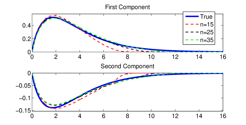
In Figure 2 we show approximation of the corresponding ground wave function associated with E0E_{0}. We have also depicted the analytical eigenfunction:

(4.2) u0​(r)=ν0​(γ(1−γ2)1/2−1)​r1−γ2​e−(γ​E0/1−γ2)​r,u_{0}(r)=\nu_{0}\begin{pmatrix}\gamma\\ (1-\gamma^{2})^{1/2}-1\end{pmatrix}r^{\sqrt{1-\gamma^{2}}}e^{-(\gamma E_{0}/\sqrt{1-\gamma^{2}})r},

where ν0\nu_{0} is chosen so that ‖u0‖=1\|u_{0}\|=1. From this picture it is clear that, at least qualitatively, u0​(r)u_{0}(r) seems to be captured quite well even for small values of nn.

We show a quantitative analysis of the calculation of u0u_{0} in Table 3. In the middle column we compute the residual on the left of (3.4) and on the last column we compute the right hand side of (3.4). It is quite remarkable that the actual residuals are over 74%74\% smaller than the error predicted by Theorem 1.

4.2. β\beta-Dependence of the sub-coulombic potential

We now investigate the case of the potential being radially symmetric and sub-coulombic: ϕsc=ϕam=0\phi_{\mathrm{sc}}=\phi_{\mathrm{am}}=0, ϕel​(r)=γ/rβ\phi_{\mathrm{el}}(r)=\gamma/r^{\beta} for β∈(0,1)\beta\in(0,1). Here −1<γ<0-1<\gamma<0. The purpose of this experiment is to show how Theorem 1 provides a priori information about Specdisc⁡(Hκ)\operatorname{Spec}_{\text{disc}}(H_{\kappa}) even for small values of nn. Note that (1.2) is guaranteed from [Tha92, Theorems 4.7 and 4.17]. Furthermore HH has infinitely many eigenvalues according to [Tha92, Theorem 4.23].

In Figure 3, we show computation of the ground state of H−1H_{-1}, for β=0.1:0.1:1\beta=0.1:0.1:1 and γ=−1/2\gamma=-1/2. As β→1−\beta\to 1^{-}, E0→0.8661E_{0}\to 0.8661, the ground eigenvalue of the coulombic Dirac operator. As β→0+\beta\to 0^{+} the eigenvalue remains above 1/21/2. Note that the family of operators HκH_{\kappa} is not analytic at β=0\beta=0 for this potential. For β=0\beta=0 the spectrum becomes

Spec(Hκ)=(−∞,−3/2]∪[1/2,∞).\operatorname{Spec}(H_{\kappa})=(-\infty,-3/2]\cup[1/2,\infty).

The vertical bars show |Im⁡(λ)||\operatorname{Im}(\lambda)|, the maximum error in the computation of E0≈Re⁡(λ)E_{0}\approx\operatorname{Re}(\lambda) given by Theorem 1. For this example we have chosen n=15n=15. Table 4 contains the data depicted in Figure 2. Observe that the error increases as β→0+\beta\to 0^{+} and β→1−\beta\to 1^{-}. This seems to be a consequence of the fact that E0E_{0} becomes closer to other spectral points at both limits, so dE0→0d_{E_{0}}\to 0.

4.3. The inverse harmonic electric potential

In this set of experiments we consider another canonical example in the theory of Dirac operators: ϕsc=ϕam=0\phi_{\mathrm{sc}}=\phi_{\mathrm{am}}=0, ϕel​(r)=γ/(1+r2)\phi_{\mathrm{el}}(r)=\gamma/(1+r^{2}) for γ<0\gamma<0. The discrete spectrum of HH is known to be finite for −1/8<γ<0-1/8<\gamma<0 and infinite for γ<−1/8\gamma<-1/8, [Kla80]. As the parameter γ\gamma decreases, we expect that eigenvalues will appear at the threshold 1, move through the gap, and leave it at -1. This dynamics is shown in Figure 4, for the ground eigenvalue of H−1H_{-1}. It is a long standing question whether the eigenvalues become resonances when they re-enter the spectrum.

In Figure 5 we depict the first three eigenfunctions of H−1H_{-1} for γ=−4\gamma=-4. They correspond to the eigenvalues E0≈−0.3955E_{0}\approx-0.3955, E1≈0.6049E_{1}\approx 0.6049 and E2≈0.9328E_{2}\approx 0.9328. See also Figure 7. Note that for γ=−4\gamma=-4, both components of the eigenfunctions appear to obey a Sturm-Liouville type oscillation hierarchy.

4.4. Upper/lower spinor component balance and approximation of eigenvalues

We now investigate the effects of “unbalancing” the basis by choosing N≠MN\not=M.

In Figure 6, we have performed the following experiment. Fix the number of degrees of freedom, dim(ℒM​N)=200\dim(\mathcal{L}_{MN})=200. Then for N=10:5:190N=10:5:190 and M=200−NM=200-N, use the quadratic method as well as the Galerkin method to approximate eigenvalues of HκH_{\kappa} in the spectral gap (−1,1)(-1,1). We firstly consider ϕsc=ϕam=0\phi_{\mathrm{sc}}=\phi_{\mathrm{am}}=0 and ϕel(r)=−1/(2r)\phi_{\mathrm{el}}(r)=-1/(2r).

The Galerkin method might or might not produce spurious eigenvalues. The quadratic method will always provide two-sided non-polluted bounds for the true eigenvalues with a residual, obtained from (3.2), which might change with NN. See also figures  4 and 6. The Galerkin method appears to pollute heavily near the upper end of the gap for N>MN>M, as predicted by the considerations of Section 2. Moreover, for the ground state, the minimal |Im⁡(λ)||\operatorname{Im}(\lambda)| is not achieved at N=100N=100 which corresponds to N=MN=M, but rather at some N>100N>100. It is remarkable that the residual are reduced significantly (up to 66%66\% for the true residual) when M⁡(N)/N≈1/5M(N)/N\approx 1/5.

If we performed the analogous experiment for the inverse harmonic potential, the conclusion are also rather surprising. See Figure 7. The Galerkin method appears to pollute heavily near the upper end of the gap for N>MN>M as predicted in Section 2. However, now the approximation is improved by over 16%16\% for E0E_{0} and over 18%18\% for E1E_{1}, if M⁡(N)/N≈3M(N)/N\approx 3.

We can explain these phenomena by considering the relation between the components of the exact eigenvectors.

In the case of a purely coulombic potential, the ground state is given by (4.2) where ν0\nu_{0} is a real constant. The lower spinor component just differs from the upper one by a scalar factor. When γ∈(0,1)\gamma\in(0,1), the lower component is smaller in modulus than the upper one. Choosing N>MN>M, can reduce an upper bound of the residual associated to the first component, while the residual associated to the second component remains small due to the smallness of the lower component.

In the case of an inverse harmonic purely electric potential, this argument fails, as the two spinor components of the eigenfunction are not a scalar factor of each other, see Figure 5. If we denote an eigenfunction by u=(uupp,ulow)u=(u^{\mathrm{upp}},u^{\mathrm{low}}), the figure suggests that |∂r2uupp​(0)|<<|∂r2ulow​(0)||\partial_{r}^{2}u^{\mathrm{upp}}(0)|<<|\partial_{r}^{2}u^{\mathrm{low}}(0)|. As |∂r2Φk​(0)|=0|\partial_{r}^{2}\Phi_{k}(0)|=0, it is natural to expect that a decrease in the residual is only achieved by choosing a suitable M>NM>N.

Remark 5.

Although we can not prove it rigourously, strong evidence suggests that (for any of the potentials considered above) no spurious eigenvalue is produced by the Galerkin method when N=MN=M. Why bothering then with more complicated procedures, such as the quadratic projection method, to avoid inexistent spectral pollution. A partial answer is, on the one hand, robustness: we do not know a priori whether the Galerkin method pollutes for a given basis. On the other hand, as the experiments of this section suggest, some times forcing a kinetic unbalance into a model might improve convergence properties.

4.5. Convergence properties of the odd Hermite basis

A convergence analysis, as the number of degrees of freedom increases, can be found in Figure 8 and Table 5. Due to the discussion of Section 4.4, we consider this for different ratios N/MN/M.

The right graph shows that the conclusion of Corollary 6 is far from optimal for the inverse harmonic potential of Section 4.3. As expected from Section 4.4, a faster convergence rate as well as smaller residuals are found if we suitably choose N<MN<M.

The left graph corresponds to the coulombic potential discussed in Section 4.1. It clearly shows that the order of convergence of λn→E\lambda_{n}\to E does not obey the estimate |λn−E|≤O⁡(n−a)|\lambda_{n}-E|\leq O(n^{-a}) (for some a>0a>0) of Corollary 4. In fact the convergence rate seems to decrease as we increase the number of degrees of freedom. This reduction in the speed of convergence can be prevented by putting M=f⁡(N)M=f(N) for a suitable non-linear increasing function 0<f⁡(x)<x0<f(x)<x. The optimal f⁡(x)f(x), however, might depend on the eigenvalue to be approximated.

Remark 6.

According to Remark 2, the actual approximate eigenvalue Re⁡(λ)\operatorname{Re}(\lambda) is correct up to O⁡(n−2​a)O(n^{-2a}), where aa is the second column of Table 5. Furthermore, note that, in the case of the coulombic potential we can compute directly the true residual |Re⁡(λ)−E||\operatorname{Re}(\lambda)-E|. From Figure 6 bottom, it is clear that this true residual is substantially smaller than the one estimated by |Im⁡(λ)||\operatorname{Im}(\lambda)|.

Appendix A Entries of the matrix polynomial coefficients

The recursive identities satisfied by the Hermite functions allow us to find recursive expressions for the matrix entries of KK and LL in (3.1) when G=HκG=H_{\kappa}. Rather than estimating the corresponding inner products by trapezoidal rules, we build the codes involved in the numerical experiments performed in Section 4 using these explicit expressions. As large factors are cancelled in these explicit expressions, this approach turns out to be far more accurate. Since some of the calculations are not entirely trivial, we include here the crucial details.

Let

T1=∫0∞Φk​(r)​Φj​(r)​𝑑r,T2​(k,j)=∫0∞Φk′​(r)​Φj​(r)​𝑑r,\displaystyle T_{1}=\int_{0}^{\infty}\Phi_{k}(r)\Phi_{j}(r)\,\mathrm{d}r,\qquad T_{2}(k,j)=\int_{0}^{\infty}\Phi_{k}^{\prime}(r)\Phi_{j}(r)\,\mathrm{d}r,
T3=∫0∞1r​Φk​(r)​Φj​(r)​𝑑r,T4=∫0∞Φk′​(r)​Φj′​(r)​𝑑r,\displaystyle T_{3}=\int_{0}^{\infty}\frac{1}{r}\Phi_{k}(r)\Phi_{j}(r)\,\mathrm{d}r,\qquad T_{4}=\int_{0}^{\infty}\Phi_{k}^{\prime}(r)\Phi_{j}^{\prime}(r)\,\mathrm{d}r,
T5​(k,j)=∫0∞1r​Φk′​(r)​Φj​(r)​𝑑r,T6=∫0∞1r2​Φk​(r)​Φj​(r)​𝑑r,\displaystyle T_{5}(k,j)=\int_{0}^{\infty}\frac{1}{r}\Phi_{k}^{\prime}(r)\Phi_{j}(r)\,\mathrm{d}r,\qquad T_{6}=\int_{0}^{\infty}\frac{1}{r^{2}}\Phi_{k}(r)\Phi_{j}(r)\,\mathrm{d}r,
F1=∫0∞ϕel​(r)​Φk​(r)​Φj​(r)​𝑑r,F2=∫0∞ϕel2​(r)​Φk​(r)​Φj​(r)​𝑑r,\displaystyle F_{1}=\int_{0}^{\infty}\phi_{\mathrm{el}}(r)\Phi_{k}(r)\Phi_{j}(r)\,\mathrm{d}r,\qquad F_{2}=\int_{0}^{\infty}\phi_{\mathrm{el}}^{2}(r)\Phi_{k}(r)\Phi_{j}(r)\,\mathrm{d}r,
F3=∫0∞ϕel​(r)r​Φk​(r)​Φj​(r)​𝑑r,F4​(k,j)=∫0∞ϕel​(r)​Φk′​(r)​Φj​(r)​𝑑r.\displaystyle F_{3}=\int_{0}^{\infty}\frac{\phi_{\mathrm{el}}(r)}{r}\Phi_{k}(r)\Phi_{j}(r)\,\mathrm{d}r,\qquad F_{4}(k,j)=\int_{0}^{\infty}\phi_{\mathrm{el}}(r)\Phi_{k}^{\prime}(r)\Phi_{j}(r)\,\mathrm{d}r.

Here and below we stress the dependence on j,kj,k when the coefficient is not symmetric with respect to these indices. Denote

Ψk,1=(Φk0),Ψj,2=(0Φj).\Psi_{k,1}=\begin{pmatrix}\Phi_{k}\\ 0\end{pmatrix},\qquad\Psi_{j,2}=\begin{pmatrix}0\\ \Phi_{j}\end{pmatrix}.

Then ⟨Hκ​Ψk​l,Ψj​m⟩\langle H_{\kappa}\Psi_{kl},\Psi_{jm}\rangle are given according to Table 1 and ⟨Hκ​Ψk​l,Hκ​Ψj​m⟩\langle H_{\kappa}\Psi_{kl},H_{\kappa}\Psi_{jm}\rangle are given according to Table 2.

m=1m=1 m=2m=2 l=1l=1 T1+F1T_{1}+F_{1} T2​(k,j)+κ​T3T_{2}(k,j)+\kappa T_{3} l=2l=2 −T2​(k,j)+κ​T3-T_{2}(k,j)+\kappa T_{3} −T1+F1-T_{1}+F_{1}

Table 1. Term ⟨Hκ​Ψk​l,Ψj​m⟩\langle H_{\kappa}\Psi_{kl},\Psi_{jm}\rangle.

m=1m=1 m=2m=2 l=1l=1 T1+T4+κ​T5​(k,j)+κ​T5​(j,k)+T_{1}+T_{4}+\kappa T_{5}(k,j)+\kappa T_{5}(j,k)+ −T2​(k,j)−T2​(j,k)+2​κ​F3+-T_{2}(k,j)-T_{2}(j,k)+2\kappa F_{3}+ κ2​T6+2​F1+F2\kappa^{2}T_{6}+2F_{1}+F_{2} F4​(k,j)−F4​(j,k)F_{4}(k,j)-F_{4}(j,k) l=2l=2 −T2​(k,j)−T2​(j,k)+2​κ​F3+-T_{2}(k,j)-T_{2}(j,k)+2\kappa F_{3}+ T1+T4−κ​T5​(k,j)−κ​T5​(j,k)+T_{1}+T_{4}-\kappa T_{5}(k,j)-\kappa T_{5}(j,k)+ −F4​(k,j)+F4​(j,k)-F_{4}(k,j)+F_{4}(j,k) κ2​T6−2​F1+F2\kappa^{2}T_{6}-2F_{1}+F_{2}

Table 2. Term ⟨Hκ​Ψk​l,Hκ​Ψj​m⟩\langle H_{\kappa}\Psi_{kl},H_{\kappa}\Psi_{jm}\rangle.

For m,n∈ℕ∪0m,n\in\mathbb{N}\cup{0}, let

P⁡(n)={∏l=1n(1+12​l)n≠01n=0P(n)=\left\{\begin{array}[]{ll}\prod_{l=1}^{n}\left(1+\frac{1}{2l}\right)&n\not=0\\ 1&n=0\end{array}\right.

and

(A.1) I⁡(m,n)=1cm​cn​∫0∞hm​(r)​hn​(r)​e−r2​𝑑r.I(m,n)=\frac{1}{c_{m}c_{n}}\int_{0}^{\infty}h_{m}(r)h_{n}(r)e^{-r^{2}}\,\mathrm{d}r.
Lemma 7.
I⁡(m,n)={δm​nm≡n​ (mod 2)(−1)k−j+1​2​P​(k)​P​(j)(2​k−2​j−1)​π⁡(2​k+1)m=2k,n=2j+1.I(m,n)=\left\{\begin{array}[]{ll}\delta_{mn}&m\equiv n\text{ (mod 2)}\\ \frac{(-1)^{k-j+1}\sqrt{2P(k)P(j)}}{(2k-2j-1)\sqrt{\pi(2k+1)}}&m=2k,\,n=2j+1.\end{array}\right.
Proof.

If m≡n​ (mod 2)m\equiv n\text{ (mod 2)}, then hm​(r)​hn​(r)h_{m}(r)h_{n}(r) is an even function for r∈ℝr\in\mathbb{R} and so

∫0∞hm​(r)​hn​(r)​e−r2​𝑑r=12​∫−∞∞hm​(r)​hn​(r)​e−r2​𝑑r.\int_{0}^{\infty}h_{m}(r)h_{n}(r)e^{-r^{2}}\,\mathrm{d}r=\frac{1}{2}\int_{-\infty}^{\infty}h_{m}(r)h_{n}(r)e^{-r^{2}}\,\mathrm{d}r.

On the other hand, if m≢n​ (mod 2)m\not\equiv n\text{ (mod 2)}, say m=2​km=2k and n=2​j+1n=2j+1, (3.10) and integration by parts yield

∫0∞h2​k​(r)​h2​j+1​(r)​e−r2​𝑑r\displaystyle\int_{0}^{\infty}h_{2k}(r)h_{2j+1}(r)e^{-r^{2}}\,\mathrm{d}r =∫0∞h2​j+1​(r)​(e−r2)(2​k)​𝑑r\displaystyle=\int_{0}^{\infty}h_{2j+1}(r)(e^{-r^{2}})^{(2k)}\,\mathrm{d}r
=−∫0∞h2​j+1′(r)(e−r2)(2​k−1)dr\displaystyle=-\int_{0}^{\infty}h_{2j+1}^{\prime}(r)(e^{-r^{2}})^{(2k-1)}\,\mathrm{d}r
=−2(2j+1)∫0∞h2​j(r)(e−r2)(2​k−1)dr\displaystyle=-2(2j+1)\int_{0}^{\infty}h_{2j}(r)(e^{-r^{2}})^{(2k-1)}\,\mathrm{d}r
=22​(j+1)​(2​k−1)​∫0∞h2​k−2​(r)​h2​j−1​(r)​e−r2​𝑑r.\displaystyle=2^{2}(j+1)(2k-1)\int_{0}^{\infty}h_{2k-2}(r)h_{2j-1}(r)e^{-r^{2}}\,\mathrm{d}r.

The corresponding expression for I⁡(m,n)I(m,n) can be obtained in a straightforward manner from these two assertions. ∎

Lemma 8.
T1​(k,j)=δj​k,T2​(k,j)=4​(−1)k−j+1​(k−j)π​(2​k−2​j−1)​(2​k−2​j+1)​P⁡(j)​P​(k),\displaystyle T_{1}(k,j)=\delta_{jk},\qquad T_{2}(k,j)=\frac{4(-1)^{k-j+1}(k-j)}{\sqrt{\pi}(2k-2j-1)(2k-2j+1)}\sqrt{P(j)P(k)},
T3​(k,j)=2​(−1)k−j+1​P⁡(j)π​P⁡(k)​∑m=0kP⁡(m)(2​m+1)​(2​m−2​j−1),\displaystyle T_{3}(k,j)=\frac{2(-1)^{k-j+1}\sqrt{P(j)}}{\sqrt{\pi}\sqrt{P(k)}}\sum_{m=0}^{k}\frac{P(m)}{(2m+1)(2m-2j-1)},
T4​(k,j)=12​{−2​k​(2​k+1)j=k−14​k+3j=k−(2​k+2)​(2​k+3)j=k+10otherwise,\displaystyle T_{4}(k,j)=\frac{1}{2}\left\{\begin{array}[]{ll}-\sqrt{2k(2k+1)}&j=k-1\\ 4k+3&j=k\\ -\sqrt{(2k+2)(2k+3)}&j=k+1\\ 0&\text{otherwise},\end{array}\right.
T5​(k,j)={2​(−1)j−k​P⁡(k)P⁡(j)k<j1k=j0k>j,T6​(k,j)=(−1)j−k​2​{P⁡(j)P⁡(k)j≤kP⁡(k)P⁡(j)k<j.\displaystyle T_{5}(k,j)=\left\{\begin{array}[]{ll}2(-1)^{j-k}\sqrt{\frac{P(k)}{P(j)}}&k<j\\ 1&k=j\\ 0&k>j,\end{array}\right.\qquad T_{6}(k,j)=(-1)^{j-k}2\left\{\begin{array}[]{ll}\sqrt{\frac{P(j)}{P(k)}}&j\leq k\\ \sqrt{\frac{P(k)}{P(j)}}&k<j.\end{array}\right.
Proof.

Let I⁡(m,n)I(m,n) be given by (A.1). By virtue of identities (3.10) and (3.11),

∫0∞h2​k+1′​h2​j+1​e−r2​𝑑r\displaystyle\int_{0}^{\infty}h_{2k+1}^{\prime}h_{2j+1}e^{-r^{2}}\,\mathrm{d}r =(2​k+1)​I​(2​k,2​j+1)−2−1​I​(2​k+2,2​j+1),\displaystyle=(2k+1)I(2k,2j+1)-2^{-1}I(2k+2,2j+1),
∫0∞1r​h2​k+1​h2​j+1​e−r2​𝑑r\displaystyle\int_{0}^{\infty}\frac{1}{r}h_{2k+1}h_{2j+1}e^{-r^{2}}\,\mathrm{d}r =∑l=0k(−1)l​22​l+1​k!(k−l)!​I​(2​(k−l),2​j+1).\displaystyle=\sum_{l=0}^{k}(-1)^{l}2^{2l+1}\frac{k!}{(k-l)!}I(2(k-l),2j+1).

This yields T2T_{2} and T3T_{3}.

Let

J⁡(k,j)=∫0∞1r​h2​k​h2​j+1​e−r2​𝑑r.J(k,j)=\int_{0}^{\infty}\frac{1}{r}h_{2k}h_{2j+1}e^{-r^{2}}\,\mathrm{d}r.

Then

J⁡(k,j)={π​22​j​(2​k)!​(−1)j−k​j!k!k≤j0k>jJ(k,j)=\left\{\begin{array}[]{ll}\frac{\sqrt{\pi}2^{2j}(2k)!(-1)^{j-k}j!}{k!}&k\leq j\\ 0&k>j\end{array}\right.

and

∫0∞1r​h2​k+1′​h2​j+1​e−r2​𝑑r=2​(2​k+1)​J​(k,j)−δk​j​π​2k​(2​k+1)!.\int_{0}^{\infty}\frac{1}{r}h_{2k+1}^{\prime}h_{2j+1}e^{-r^{2}}\,\mathrm{d}r=2(2k+1)J(k,j)-\delta_{kj}\sqrt{\pi}2^{k}(2k+1)!.

This renders T5T_{5}. Moreover, integration by parts ensures

T6=∫0∞1r2ΦkΦj=−∫0∞(1r)′ΦkΦj=(T5(k,j)+T5(j,k)).T_{6}=\int_{0}^{\infty}\frac{1}{r^{2}}\Phi_{k}\Phi_{j}=-\int_{0}^{\infty}\Big(\frac{1}{r}\Big)^{\prime}\Phi_{k}\Phi_{j}=\big(T_{5}(k,j)+T_{5}(j,k)\big).

The expression for T4T_{4} follows from (3.13) and the identity

∫0∞Φk′(r)Φj′(r)dr=12∫−∞∞−Φk′′(r)Φj(r)dr.\int_{0}^{\infty}\Phi_{k}^{\prime}(r)\Phi_{j}^{\prime}(r)\,\mathrm{d}r=\frac{1}{2}\int_{-\infty}^{\infty}-\Phi_{k}^{\prime\prime}(r)\Phi_{j}(r)\,\mathrm{d}r.

∎

From E1E_{1} and E2E_{2} in the next lemma, one easily obtains explicit formulae for FnF_{n} when ϕel​(r)=γ/rβ\phi_{\mathrm{el}}(r)=\gamma/r^{\beta}.

Lemma 9.

For β∈[0,1]\beta\in[0,1] and α∈[−1,2]\alpha\in[-1,2], let

E1​(β,k,j)=∫0∞1rβ​Φk′​(r)​Φj​(r)​𝑑r,E2​(α,k,j)=∫0∞1rα​Φk​(r)​Φj​(r)​𝑑r.E_{1}(\beta,k,j)=\int_{0}^{\infty}\frac{1}{r^{\beta}}\Phi_{k}^{\prime}(r)\Phi_{j}(r)\,\mathrm{d}r,\qquad E_{2}(\alpha,k,j)=\int_{0}^{\infty}\frac{1}{r^{\alpha}}\Phi_{k}(r)\Phi_{j}(r)\,\mathrm{d}r.

Then

E1​(β,k,j)=(2​j+1)​E2​(β+1,k,j)+2​(2​j+1)​j​E2​(β+1,k,j−1)−E2​(β−1,k,j)E_{1}(\beta,k,j)=(2j+1)E_{2}(\beta+1,k,j)+\sqrt{2(2j+1)j}E_{2}(\beta+1,k,j-1)-E_{2}(\beta-1,k,j)

and

E2​(α,k,j)=2​P​(j)​P​(k)​(−1)k+jπ​∑m,p=1k,j(−1)m+p​Γ​(3−α2+m+p)​(km)​(jp)m!​p!​P​(m)​P​(p).E_{2}(\alpha,k,j)=\frac{2P(j)P(k)(-1)^{k+j}}{\sqrt{\pi}}\sum_{m,p=1}^{k,j}\frac{(-1)^{m+p}\Gamma(\frac{3-\alpha}{2}+m+p)\begin{pmatrix}k\\ m\end{pmatrix}\begin{pmatrix}j\\ p\end{pmatrix}}{m!p!P(m)P(p)}.
Proof.

Let

Sn​(k)=c2​k+1−1​(2​k+1)!​(−1)k−n​22​n+1(k−n)!​(2​n+1)!.S_{n}(k)=c_{2k+1}^{-1}(2k+1)!\frac{(-1)^{k-n}2^{2n+1}}{(k-n)!(2n+1)!}.

Then

c2​k+1−1​h2​k+1​(r)=∑n=0kSn​(k)​r2​n+1c_{2k+1}^{-1}h_{2k+1}(r)=\sum_{n=0}^{k}S_{n}(k)r^{2n+1}

and

E2​(α,k,j)=∑m,p=1k,jSm​(k)​Sp​(j)​K​(α,m,p)E_{2}(\alpha,k,j)=\sum_{m,p=1}^{k,j}S_{m}(k)S_{p}(j)K(\alpha,m,p)

where

K⁡(α,m,p)=∫0∞1rα​r2​m+1​r2​p+1​e−r2​𝑑r=12​Γ​(3−α2+m+p).K(\alpha,m,p)=\int_{0}^{\infty}\frac{1}{r^{\alpha}}r^{2m+1}r^{2p+1}e^{-r^{2}}\,\mathrm{d}r=\frac{1}{2}\Gamma\Big(\frac{3-\alpha}{2}+m+p\Big).

On the other hand, the expression for E1E_{1} follows from applying (3.10) and (3.11). ∎

If E3E_{3} and E4E_{4} are as in the following lemma and ϕel​(r)=11+r2\phi_{\mathrm{el}}(r)=\frac{1}{1+r^{2}}, then

F1​(k,j)\displaystyle F_{1}(k,j) =E3​(2​k+1,2​j+1),\displaystyle=E_{3}(2k+1,2j+1),
F2​(k,j)\displaystyle F_{2}(k,j) =12​(2​k+12​E4​(2​k,2​j+1)+2​j+12​E4​(2​k+1,2​j)CLOSE\displaystyle=\frac{1}{2}\Big(\sqrt{\frac{2k+1}{2}}E_{4}(2k,2j+1)+\sqrt{\frac{2j+1}{2}}E_{4}(2k+1,2j)
−k+1​E4​(2​k+2,2​j+1)−j+1​E4​(2​k+1,2​j+2)+\displaystyle\qquad-\sqrt{k+1}E_{4}(2k+2,2j+1)-\sqrt{j+1}E_{4}(2k+1,2j+2)+
OPENE3​(2​k+1,2​j+1)),\displaystyle\qquad E_{3}(2k+1,2j+1)\Big),
F3​(k,j)\displaystyle F_{3}(k,j) =T3​(k,j)−2​k+12​E3​(2​k,2​j+1)−k+1​E3​(2​k+2,2​j+1),\displaystyle=T_{3}(k,j)-\sqrt{\frac{2k+1}{2}}E_{3}(2k,2j+1)-\sqrt{k+1}E_{3}(2k+2,2j+1),
F4​(k,j)\displaystyle F_{4}(k,j) =2​k+12​E3​(2​k,2​j+1)−k+1​E3​(2​k+2,2​j+1).\displaystyle=\sqrt{\frac{2k+1}{2}}E_{3}(2k,2j+1)-\sqrt{k+1}E_{3}(2k+2,2j+1).
Lemma 10.

For m,n∈ℕ∪{0}m,n\in\mathbb{N}\cup\{0\}, let I⁡(m,n)I(m,n) be as in Lemma 7,

E3​(m,n)\displaystyle E_{3}(m,n) =1cm​cn​∫0∞11+r2​hm​(r)​hn​(r)​e−r2​𝑑r,\displaystyle=\frac{1}{c_{m}c_{n}}\int_{0}^{\infty}\frac{1}{1+r^{2}}h_{m}(r)h_{n}(r)e^{-r^{2}}\,\mathrm{d}r,
E4​(m,n)\displaystyle E_{4}(m,n) =1cm​cn​∫0∞r1+r2​hm​(r)​hn​(r)​e−r2​𝑑r.\displaystyle=\frac{1}{c_{m}c_{n}}\int_{0}^{\infty}\frac{r}{1+r^{2}}h_{m}(r)h_{n}(r)e^{-r^{2}}\,\mathrm{d}r.

Then

E3​(0,0)\displaystyle E_{3}(0,0) =2​e​∫01e−t2​𝑑t+e​π,\displaystyle=2e\int_{0}^{1}e^{-t^{2}}\,\mathrm{d}t+e\sqrt{\pi},
E4​(0,0)\displaystyle E_{4}(0,0) =e​π​∫1∞e−tt​𝑑t,\displaystyle=e\sqrt{\pi}\int_{1}^{\infty}\frac{e^{-t}}{t}\,\mathrm{d}t,
E3​(m+1,0)\displaystyle E_{3}(m+1,0) =1m+1​(E4​(m,0)−m​E3​(m−1,0)),\displaystyle=\frac{1}{\sqrt{m+1}}\big(E_{4}(m,0)-\sqrt{m}E_{3}(m-1,0)\big),
E4​(m+1,0)\displaystyle E_{4}(m+1,0) =1m+1​(2​I​(m,0)−2​E3​(m,0)−m​E4​(m−1,0)),\displaystyle=\frac{1}{\sqrt{m+1}}\left(\sqrt{2}I(m,0)-\sqrt{2}E_{3}(m,0)-\sqrt{m}E_{4}(m-1,0)\right),
E3​(m+1,n+1)\displaystyle E_{3}(m+1,n+1) =1(m+1)​(n+1)​(2​I​(m,n)−2​E3​(m,n)+CLOSE\displaystyle=\frac{1}{\sqrt{(m+1)(n+1)}}\big(2I(m,n)-2E_{3}(m,n)+
OPEN−2​m​E4​(m−1,n)−2​n​E4​(m,n−1)+m​n​E3​(m−1,n−1))\displaystyle\qquad-\sqrt{2m}E_{4}(m-1,n)-\sqrt{2n}E_{4}(m,n-1)+\sqrt{mn}E_{3}(m-1,n-1)\big)
E4​(m+1,n+1)\displaystyle E_{4}(m+1,n+1) =1(m+1)​(n+1)​(2​(n+1)​I​(m,n+1)−2​E4​(m,n)+CLOSE\displaystyle=\frac{1}{\sqrt{(m+1)(n+1)}}\left(\sqrt{2(n+1)}I(m,n+1)-2E_{4}(m,n)+\right.
OPEN2​n​E3​(m,n−1)−2​m​E4​(m−1,n)+m​n​E3​(m−1,n−1)).\displaystyle\qquad\left.\quad\sqrt{2n}E_{3}(m,n-1)-\sqrt{2m}E_{4}(m-1,n)+\sqrt{mn}E_{3}(m-1,n-1)\right).
Proof.

The recursions for E3E_{3} and E4E_{4}, follow from (3.11). ∎

Acknowledgements

The authors would like to thank Jean Dolbeault, Mathieu Lewin, Michael Levitin and Éric Séré for fruitful discussions during the preparation of this work.

The first author is grateful for the hospitality of CEREMADE and Université de Franche-Comté. The second author has been partially supported by ESPRC grant EP/D054621.

References

  • [BG87] A. Berthier and V. Georgescu. On the point spectrum of Dirac operators. J. Funct. Anal., 71(2):309–338, 1987.
  • [BHM+] Timo Betcke, Nicholas J. Higham, Volker Mehrmann, Christian Schröder, and Françoise Tisseur. NLEVP: A collection of nonlinear eigenvalue problems. http://www.mims.manchester.ac.uk/research/numerical-analysis/nlevp.html.
  • [BHM+08] Timo Betcke, Nicholas J. Higham, Volker Mehrmann, Christian Schröder, and Françoise Tisseur. NLEVP: A collection of nonlinear eigenvalue problems. MIMS EPrint 2008.40, Manchester Institute for Mathematical Sciences, The University of Manchester, UK, April 2008.
  • [BL94] Mikhail Sh. Birman and Ari Laptev. Discrete spectrum of the perturbed Dirac operator. Ark. Mat., 32(1):13–32, 1994.
  • [BL07] Lyonell Boulton and Michael Levitin. On approximation of the eigenvalues of perturbed periodic schrodinger operators. J. Phys. A: Math. Theor., 40:9319–9329, 2007.
  • [Bou06] Lyonell Boulton. Limiting set of second order spectra. Math. Comp., 75(255):1367–1382, 2006.
  • [Bou07] Lyonell Boulton. Non-variational approximation of discrete eigenvalues of self-adjoint operators. IMA J. Numer. Anal., 27(1):102–121, 2007.
  • [DEL07] Jean Dolbeault, Maria J. Esteban, and Michael Loss. Relativistic hydrogenic atoms in strong magnetic fields. Ann. Henri Poincaré, 8(4):749–779, 2007.
  • [DES00] Jean Dolbeault, Maria J. Esteban, and Eric Séré. On the eigenvalues of operators with gaps. Application to Dirac operators. J. Funct. Anal., 174(1):208–226, 2000.
  • [DES03] Jean Dolbeault, Maria J. Esteban, and Eric Séré. A variational method for relativistic computations in atomic and molecular physics. Int. J. Quantum Chemistry, 93:149–155, 2003.
  • [DESV00] Jean Dolbeault, Maria J. Esteban, Eric Séré, and Michael Vanbreugel. Minimization methods for the one-particle dirac equation. Phys. Rev. Letters, 85:4020–4023, 2000.
  • [Dya90] Kenneth Dyall. Kinetic balance and variational bounds failure in the solution of the dirac equation in a finite gaussian basis set. Chem. Phys. Letters, 174(1):25–32, 1990.
  • [GL99] Marcel Griesemer and Joseph Lutgen. Accumulation of discrete eigenvalues of the radial Dirac operator. J. Funct. Anal., 162(1):120–134, 1999.
  • [His00] P. D. Hislop. Exponential decay of two-body eigenfunctions: a review. In Proceedings of the Symposium on Mathematical Physics and Quantum Field Theory (Berkeley, CA, 1999), volume 4 of Electron. J. Differ. Equ. Conf., pages 265–288 (electronic), San Marcos, TX, 2000. Southwest Texas State Univ.
  • [Kla80] M. Klaus. On the point spectrum of Dirac operators. Helv. Phys. Acta., 53:463–482, 1980.
  • [LLT02] Heinz Langer, Matthias Langer, and Christiane Tretter. Variational principles for eigenvalues of block operator matrices. Indiana Univ. Math. J., 51(6):1427–1459, 2002.
  • [LS04] Michael Levitin and Eugene Shargorodsky. Spectral pollution and second-order relative spectra for self-adjoint operators. IMA J. Numer. Anal., 24(3):393–416, 2004.
  • [Sch03] Karl Michael Schmidt. Eigenvalue asymptotics of perturbed periodic Dirac systems in the slow-decay limit. Proc. Amer. Math. Soc., 131(4):1205–1214 (electronic), 2003.
  • [SH84] Richard Stanton and Stephen Havriliak. Kinetic balance a partial solution to the problem of variational safety in dirac calculations. J. Chem. Phys., 81(4):1910–1918, 1984.
  • [Sha00] Eugene Shargorodsky. Geometry of higher order relative spectra and projection methods. J. Operator Theory, 44(1):43–62, 2000.
  • [Str08] Michael Strauss. Quadratic projection methods for approximating the spectrum of self-adjoint operators. Preprint, 2008.
  • [Tha92] Bernd Thaller. The Dirac Equation. Springer-Verlag, Berlin, 1992.
  • [Tri99] Hans Triebel. Hardy inequalities in function spaces. Math. Bohem., 124(2-3):123–130, 1999.
Refer to caption
Figure 1. Portion of Spec2⁡(H−1,ℒn)\operatorname{Spec}_{2}(H_{-1},\mathcal{L}_{n}) in thin boxes around [−3,3][-3,3] for the purely coulombic potential with γ=−1/2\gamma=-1/2. The bottom image shows details of the picture near 11. Here we superimpose two values of nn, 500500 and 10001000. According to Theorem 1 there are approximate energy states at E≈0.8661±0.0236E\approx 0.8661\pm 0.0236, E≈0.9662±0.0086E\approx 0.9662\pm 0.0086 and E≈0.9853±0.0041E\approx 0.9853\pm 0.0041. These correspond to the actual eigenvalues E0≈0.866025E_{0}\approx 0.866025, E1≈0.965925E_{1}\approx 0.965925 and E2≈0.985121E_{2}\approx 0.985121.

Refer to caption

Figure 2. Approximate ground wave function for a purely coulombic potential with γ=−1/2\gamma=-1/2. The true wave function (blue line) can be found explicitly, [Tha92, Section 7.4.2]. The ground state in this case is E0=1−γ2≈0.866025E_{0}=\sqrt{1-\gamma^{2}}\approx 0.866025. We have deliberately chosen small dimensions nn for the test spaces, in order to illustrate approximation of the method. The residual error is actually much smaller that the one predicted by Theorem 1, see Table 3.

nn ‖v−Πℰ​v‖‖v‖\frac{\|v-\Pi_{\mathcal{E}}v\|}{\|v\|} |Im⁡(λ)|dE\frac{|\operatorname{Im}(\lambda)|}{d_{E}} 1515 0.1761150.176115 0.6805990.680599 2525 0.0845270.084527 0.5142050.514205 3535 0.0725520.072552 0.4570340.457034

Table 3. Here we compare both sides of (3.4), for the computation of the approximate eigenfunctions of Figure 2. We approximate dE=E1−E0≈0.0999004d_{E}=E_{1}-E_{0}\approx 0.0999004.

Refer to caption

Figure 3. Computation of the ground energy value for H−1H_{-1} and ϕel​(r)=−12​rβ\phi_{\mathrm{el}}(r)=-\frac{1}{2r^{\beta}}. We depict E0E_{0} against β\beta. The vertical bars correspond to the error predicted by Theorem 1.

β\beta E0E_{0} Im⁡(λ)\operatorname{Im}(\lambda) 0.1 0.6474 0.0675 0.2 0.6932 0.0599 0.3 0.7316 0.0542 0.4 0.7642 0.0499 0.5 0.7918 0.0468 0.6 0.8151 0.0448 0.7 0.8346 0.0439 0.8 0.8505 0.0449 0.9 0.8627 0.0504 1.0 0.8711 0.0680

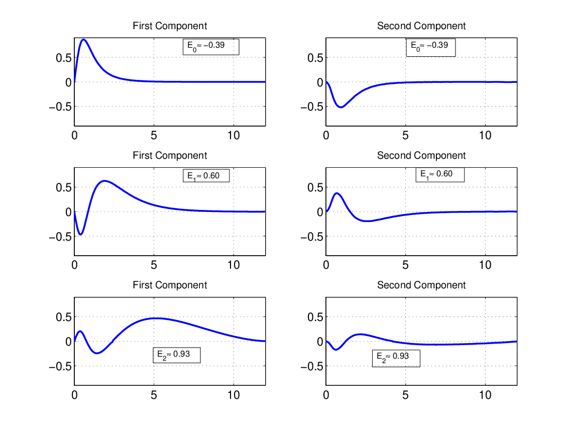
Table 4. Data depicted in Figure 3

Refer to caption

Figure 4. The graph captures the evolution of E0E_{0} as it crosses the spectral gap of H−1H_{-1} where ϕel​(r)=γ/(1+r2)\phi_{\mathrm{el}}(r)=\gamma/(1+r^{2}) for γ=−5:.5:0\gamma=-5:.5:0. We consider three choices of pairs (N,M)(N,M) such that dim(ℒN​M)=120\dim(\mathcal{L}_{NM})=120. The curve corresponds to Re⁡(λn)\operatorname{Re}(\lambda_{n}) for λ=λn\lambda=\lambda_{n} in (3.4) and (3.15). The vertical bars on the curve measure |Im⁡(λn)||\operatorname{Im}(\lambda_{n})| . We superimpose the image with the eigenvalues of LL in (3.1) for G=H−1G=H_{-1}, that is the Galerkin approximation.

Refer to caption

Figure 5. Here we use Theorem 1 to find the first three eigenfunctions of H−1H_{-1} with ϕel(r)=−4/(1+r2)\phi_{\mathrm{el}}(r)=-4/(1+r^{2}). The numerical evidence suggests: E0≈−0.3955E_{0}\approx-0.3955, E1≈0.6049E_{1}\approx 0.6049 and E2≈0.9328E_{2}\approx 0.9328.

Refer to caption

Figure 6. Here E0E_{0} and E1E_{1} are eigenvalues of H−1H_{-1} for ϕel​(r)=−12​r\phi_{\mathrm{el}}(r)=-\frac{1}{2r}. The top graph shows the eigenvalues of LL in (3.1) (that is the Galerkin approximation) for G=H−1G=H_{-1} and (M,N)=(N,200−N)(M,N)=(N,200-N) so that dim(ℒN​M)=200\dim(\mathcal{L}_{NM})=200. The bottom graph depicts the residuals |Im⁡(λn)||\operatorname{Im}(\lambda_{n})| and |Re⁡(λ)−Ej||\operatorname{Re}(\lambda)-E_{j}|. For E0E_{0}, the minimum of the residual curve corresponding to |Im⁡(λ)||\operatorname{Im}(\lambda)| is achieved when N≈155N\approx 155 and it is roughly 7%7\% smaller than when N=100N=100. For the same eigenvalue, the residual curve corresponding to |Re⁡(λ)−E0||\operatorname{Re}(\lambda)-E_{0}| achieves its minimum when N=165N=165 and it is roughly 66%66\% smaller than when N=100N=100.

Refer to caption

Figure 7. Here E0,E1E_{0},\,E_{1} and E2E_{2}, are the first three eigenvalues of H−1H_{-1} for ϕel(r)=−4/(1+r2)\phi_{\mathrm{el}}(r)=-4/(1+r^{2}). The top graph shows approximation of E0≈−0.3955E_{0}\approx-0.3955, E1≈0.6049E_{1}\approx 0.6049 and E2≈0.9328E_{2}\approx 0.9328, for (M,N)=(N,120−N)(M,N)=(N,120-N) so that dim(ℒN​M)=120\dim(\mathcal{L}_{NM})=120. The curves correspond to Re⁡(λn)\operatorname{Re}(\lambda_{n}) for λ=λn\lambda=\lambda_{n} in (3.4) and (3.15). The vertical bars measure |Im⁡(λn)||\operatorname{Im}(\lambda_{n})|. The image is superimposed with the eigenvalues of LL in (3.1) for G=H−1G=H_{-1}, that is the Galerkin approximation. The bottom graph depicts the residuals |Im⁡(λn)||\operatorname{Im}(\lambda_{n})|.

Refer to caption Refer to caption

Figure 8. Log-log plots of |Im⁡(λ)||\operatorname{Im}(\lambda)| for Re⁡(λ)\operatorname{Re}(\lambda) close to an eigenvalue, E0E_{0}, for different choices of pairs (N,M)(N,M) as n=N+Mn=N+M increases. Left: κ=−1\kappa=-1, ϕel​(r)=−12​r\phi_{\mathrm{el}}(r)=-\frac{1}{2r} and E0≈0.86602E_{0}\approx 0.86602. Right: κ=−1\kappa=-1, ϕel​(r)=−21+r2\phi_{\mathrm{el}}(r)=-\frac{2}{1+r^{2}} and E0≈0.61399E_{0}\approx 0.61399. See Table 5.

NN aa bb n/8n/8 -0.6736 1.6766 n/4n/4 -0.5426 0.6555 3​n/83n/8 -0.4385 0.3530 n/2n/2 -0.3963 0.2703 5​n/85n/8 -0.5064 0.4478 3​n/43n/4 -0.6903 1.1115 7​n/87n/8 -0.9609 5.4520      NN aa bb n/8n/8 -1.3241 8.8276 n/4n/4 -0.9135 1.1303 3​n/83n/8 -0.7990 0.7223 n/2n/2 -0.7979 0.8155 5​n/85n/8 -0.8125 1.0825 3​n/43n/4 -0.8163 1.5171 7​n/87n/8 -0.8004 2.4558

Table 5. In this table we fit by least squares the data of Figure 8 and find aa and bb such that |λn−E0|≤|Im⁡(λn)|∼b​na|\lambda_{n}-E_{0}|\leq|\operatorname{Im}(\lambda_{n})|\sim bn^{a} for n=N+Mn=N+M.