Boundary conformal field theories and loop models
Abstract
We propose a systematic method to extract conformal loop models for rational conformal field theories (CFT). Method is based on defining an ADE model for boundary primary operators by using the fusion matrices of these operators as adjacency matrices. These loop models respect the conformal boundary conditions. We discuss the loop models that can be extracted by this method for minimal CFTs and then we will give dilute loop models on the square lattice as examples for these loop models. We give also some proposals for WZW models.
Keywords: Critical Loop, Bondary CFT, ADE Models
1 Introduction
The study of statistical models related to loop models is interesting both from the physical and the mathematical point of views. Most of the statistical models studied in physics such as the Ising, the q-state Potts model and also complicated vertex models can be represented in terms of loops [1]. The loop representation of the spin system is very easy to understand: loops correspond to domain walls separating regions of different magnetization. The study of critical loop models can be interesting from many point of views: they are good candidates for the ground state of topological quantum systems [2], they are also good candidates for the Schramm Loewner evolution (SLE), a method discovered by Schramm [3] to classify conformally invariant curves connecting two distinct boundary points in a simply connected domain.
Different applications of conformal loop models are stimulating to do a systematic study of these models by CFT. Recently we proposed in [4] a method to extract loop models corresponding to a conformal field theory (CFT), the method was based on defining a RSOS model for every primary operator by using fusion matrix of the primary operator as an adjacency matrix and then extracting the loop model corresponding to domain walls of the RSOS model. The weight of the loop model is equal to the quantum dimension of the corresponding operator. In this paper we want to follow the same method consistent with the conformal boundary operators, since the SLE is a boundary CFT we think that using the fusion matrix of boundary operators as an adjacency matrix is more consistent with the nature of SLE. Recently a very nice and strong project was initiated by Jacobsen and Saleur [5] followed by Dubail, Jacobsen, Saleur [6] to classify all the possible conformal boundary loop models. It is based on classifying the possible boundary loop models compatible with the boundary conformal field theories. This classification is in close relation with the earlier work by Cardy on formulating the modular invariant partition function of model on the annulus [7]. The results that we get by our method apart from simplicity are all compatible with the results in [5, 6, 7].
The paper is organized as follows: In the next section we will introduce the necessary ingredients to find the boundary operators and also the fusion matrices corresponding to them. In the third section we briefly review the method proposed in [4] and we will also generalize it to the graphs with largest eigenvalue bigger than two. The central claim of this section is as follows: the loop model extracted with this method is connected with the properties of the statistical loop model in the same universality class as the corresponding CFT. In the third section we follow explicitly some examples in particular; Ising model, tri-critical Ising model, three states Potts model and tri-critical three states Potts model. Then we will give the possible loop models, extractable with this method, of minimal CFTs and also the lattice models corresponding to these loop models. We will close this section by giving some proposals for possible loop models for WZW models. Last section contains our conclusions with a brief description of the work in progress motivated by these results.
2 Boundary conformal field Theory
To define loop model for a generic minimal CFT consistent with the conformal boundary we need to first summarize the main important facts about boundary CFT. The most important ingredient to classify the boundary conformal operators is the modular invariant partition function of the CFT. The classification of modular invariant partition functions of minimal models are well known and can be related to a pair of simply laced Dynkin diagrams [8]. The complete classification based on ADE diagrams is
| (2.1) |
where and are the Coxeter numbers of and with . The above pair of Dynkin diagrams describes bulk modular invariant partition function with some primary operators and with the following central charge
| (2.2) |
Each of the unitary minimal models with can be realized as the continuum scaling limit of an integrable two-dimensional lattice model at criticality, with heights living on the nodes of the graph . In particular, the critical series with is associated with the A-D-E lattice models [9] and the tri-critical series with is associated with the dilute lattice models [10, 11]. For theories with a diagonal torus partition function it is known that there is a conformal boundary condition associated to each operator in the theory [12]. The fusion rules of these boundary operators are just given by the bulk fusion algebra. It was shown in a series of papers that for minimal models one can propose a complete set of conformal boundary operators , where and are nodes on the Dynkin diagram of and respectively with the identification , where is an automorphism acting on the nodes of the graph . This automorphism is identity except for the , and which is symmetry of Dynkin diagram, symmetries of Dynkin diagrams play an important rule in the forthcoming discussion. Following [13] we show the corresponding operators by and the independent boundary states by which is called Cardy states. Cardy states can be written in terms of Ishibashi states, i.e. , as follows , where sum is over all Ishibashi states. We are interested to the fusion rules of these boundary operators. To give a formula for the fusion rules of these operators we need to define some quantities. Let be the eigenvectors of the adjacency matrix corresponding to the group then the graph fusion matrices with can be defined as follows
| (2.3) |
where denotes the set of exponents of , see table 1. Let’s show also the graph fusion matrix for by then following [13] the fusion rules for boundary operators are
| (2.4) |
where has the following relation with the graph fusion matrices of and
| (2.5) |
For more details about the connection of the boundary operators to
bulk counterparts see [13, 14].
| Dynkin Diagram | Coexter Number() | Coexter Exponent() |
|---|---|---|
To calculate the fusion matrices of boundary operators we need also to define a conjugation operator , it is the identity except for graphs where the eigenvectors are complex and conjugation corresponds to the Dynkin diagram automorphism. It then follows that . The operator acts on the right to raise and lower indices in the fusion matrices so it is the important ingredient to get the right fusion matrices for the boundary operators, in particular for the graphs. we will give some examples in section 4, in particular we use the above method to get the fusion matrices of the boundary operators of Ising model, tri-critical Ising model, 3 state Potts model and tri-critical 3 state Potts model.
3 Loop Models for Boundary operators
In this section we propose a method to extract some possible loop models for CFTs, the method is the same as the method introduced recently in [4]. In that reference we showed that using the fusion matrix as an adjacency matrix it is possible to associate a loop model to every primary operator. The method is briefly as follows: The graph of a primary operator has vertices where is the number of primary operators in the theory and edges connecting pairs of vertices when . Following [24] one can define a height model on the triangular lattice by imposing that the height at the site can take values . Then constraint the heights at neighboring sites according to the incidence matrix associated to a given primary field : only neighbor heights and with are admissible. For a consistent definition of loop models on a triangular lattice at least two of the heights at the corners of an elementary triangular plaquette should be equal then the weights for the elementary plaquette are defined as follows. If the heights of plaquette are with then the weight is , where satisfies . It means that the th element of the eigenvector of with eigenvalue is given by . If the heights are all equal then the weight is except for those with that have weights or depending on the particular model considered 11 1 For more details specially about identical neighbor heights see [4].. The next step is to mark triangles with unequal heights drawing a curved segment on the dual honeycomb lattice [24] and linking to the center the midpoints of the two edges with different heights ( and ) at the extremes (See fig 1). Summing over the admissible values of heights consistent with a given loop configuration we find
| (3.1) |
where the sum is just over . We take most of the times to get the largest eigenvalue of to guaranty positive real weights in our height models, however, we will also point to other cases.

The weight of the loops is given by the largest eigenvalue of the fusion matrix and the partition function of the model is as follows
| (3.2) |
where is the number of bonds in the loop configuration and is the number of loops. Using this method we can correspond to every boundary conformal operator a loop model, since the model posses a dilute critical point for with ; see [15], correspondingly our loop models will have a critical point just for the fields with smaller than . The model has another critical regime, the so-called dense phase, for corresponds to a different universality class. Mapping to the model helps us to find the connection with SLE: from coulomb gas arguments we know that, in the dilute regime, the loop weight has the following relation with the drift in the SLE equation
| (3.3) |
For the dense phase the above equation is still true if we work in the region . Using the above equation we can find the properties of the loop model corresponding to a boundary conformal operator. The achievement of this method is respecting the Cardy’s equation [12]: fields in the same sector have the same loop representation.
Before generalizing the definition to more general graphs we should stress that although we started with well defined minimal CFT but the loop model that we extracted is not necessarily minimal. The point is that the extracted loop model respects some aspects of the corresponding conformal field theory. This is like to say that although the domain walls in Ising model at the critical point is the same as the critical but the Ising conformal field theory does not explain all the aspects of the critical curves. From this point the loop model that one can get by this method from the rational CFT is not perfectly equal to the corresponding CFT.
One can generalize the above idea to the decomposable fusion graphs by the method that was explained in [16]. Since the fusion graphs of some operators in minimal models are equivalent to the tensor product of two adjacency diagrams one can use this method to extract new loop models that can also have configurations with crossing loop segments. The general strategy is based on extracting critical loop models with for the graphs with largest eigenvalue bigger than 2. Some graphs obey simple decomposition, can be written as tensor product, but others need to be mapped to simple decomposable graphs by going to the ground state adjacency graph [16]. Here we just comment on decomposable graphs , where and are simple ADE diagrams. In these cases we can define two-flavor loop model living on the honeycomb lattice independently, one is related to the loop model of with weight and the other comes from the graph with weight . Fendley showed [16] that in this case it is also possible to define consistently interacting loop model on the square lattice with partition function , where are the numbers of each kind of loop and is the number of plaquettes with a resolved potential crossing at their center. The critical values of were calculated in [17] but the critical properties of the loops are still unsolved. This is obviously is not the only method to define loop model for non-simple graphs, the other method is based on the multi-flavor loop model of [11]. In this loop model a curve of flavor separating two neighboring sites does not necessarily separate two sites with different heights, for the definition of the RSOS model in this case and its relation to the loop model see [11].
In the next section we summarize some simple examples including the most familiar minimal conformal models such as Ising, tri-critical Ising, 3-state Potts model and tri-critical 3-state Potts model. The main point is to take the fusion graphs as adjacency graphs in the consistent way and to extract some loop models. These loop models are not equivalent to the corresponding conformal field theory but still carry some aspects of the underlying field theory in the consistent way, in particular the critical properties of these loop models are in close connection with the corresponding conformal field theory.
In this paper some distinctions are crucial. We have some minimal conformal field theories with well defined fusion matrices and modular invariant partition functions, one example is Ising conformal field theory. There are some statistical models such as spin models, RSOS models which at the critical point can be describe partially by the minimal CFT, so the Ising CFT is different from the statistical Ising model. We prefer also to distinguish between for example dilute ADE models and dilute loop model. They can be mapped to each other and have the same phase transitions but since the fundamental objects in one side is local and in the other one is non-local this distinction is useful. There are lots of work done on connecting these two models, minimal conformal field theories and statistical models counterparts, using integrability methods and our argument hardly has something new to say from this point of view. Finally we are defining another statistical model by using the fusion matrices of primary operators of conformal field theory which most of the times is in the same universality class as the statistical model counterpart of the corresponding CFT. These height models have also loop representations. This similarity can be useful to get an idea about the loop properties of the statistical models with well-known minimal CFTs.
4 Some Examples
In this section we apply the method introduced in section 3 to the
minimal conformal field theories with well defined fusion structure
and also WZW models. We will also point on the
consistency of these loop models with the Cardy’s boundary states.
These consistency is a hint to believe that it may be possible to
extend the results in to the level of the boundary partition
function [7]. For notational convenience in this section
of the paper we will drop the hat of boundary operators.

Ising model: The simplest example is the Ising model since the model has diagonal modular invariant partition function the fusion matrices of the boundary operators is the same as the bulk case. The fusion graphs are as fig 2 so the boundary states are as follows
| (4.4) |
These equations reflect the symmetry corresponding to
changing the sign of spin, this is also evident in the loop
representation; . Both operators give
, these loops are the domain walls between different
spins. It is worth mentioning that this symmetry comes from the
natural symmetry of Dynkin diagram. The operator
with corresponds to free boundary condition.
The loops in the dense phase have and describe
the domain walls of Fortuin-Kasteleyn (FK) clusters. In the above
calculation we considered only the largest eigenvalue of the fusion
graphs, however, it is also possible to consider other eigenvalues
as the weight of the loops, the cost is accepting complex local
Boltzmann weights for the corresponding height model. Since loop
models are generically non-local theories accepting complex
Boltzmann weights is equal to accepting non-unitary theories. By
this introduction one can accept the possibility of loop models with
for the loop model corresponding to the
diagram of spin operator.
Tri-critical Ising model: The next simple example is the tri-critical Ising model, which we have diagonal modular invariant partition function. The boundary CFT of this model was discussed in [18]. There are 6 boundary operators and with the fusion graphs as fig 3 and the following Cardy states
| (4.5) |
where and . The boundary states corresponding to boundary operators and can be transformed to each other by just changing the sign of spin operators, i.e. symmetry. They have also the same loop weight comes from the largest eigenvalue of the fusion matrix22 2 To get the loop weights we consider one simply connected part of the fusion graph as an adjacency graph, the other parts of the graph have always equal largest eigenvalues. One can see that these different parts are folding or orbifold dual of each other, see [19] . The boundary states and are connected also by just changing the the sign of spin states. The weight of the loops is with in the dense phase. This loop model corresponds to the boundary of geometric clusters at the geometric critical point of tri-critical Ising model or Blume-Capel model [20]. The operator describes a loop model with corresponding to in the dense phase which is related to the boundary of spin clusters and also vacancy clusters in Blume-Capel model [20, 21]. The interesting point for tri-critical models is the equality of critical exponents for spin clusters and FK clusters [20, 21].

The operator is related to the degenerate boundary condition and the corresponding loop model with is non-critical, however, it is easy to see that the fusion matrix of this operator is decomposable to simple matrices so one can define for this graph two-flavor loop model with weights and . One can conclude from the above discussion that those operators with the same loop representations are connected to each other by folding and orbifold duality and it is also possible to see these symmetries in the level of boundary states.
Similar to the previous subsection one can also consider other
possible loop weights come from the other eigenvalues of the fusion
matrix. The eigenvalues of the fusion matrix of the operator
are
and
the eigenvalues of the fusion matrix of the operator are
. The eigenvalues of the other operators are a subset
of the above eigenvalues. Interestingly apart from the negative
eigenvalues the above weights can be fitted with the boundary loop
weights in [5, 6].

Three states Potts model: The next example is the first non-diagonal case, 3-state Potts model with 8 boundary operators and , see [12, 13, 22]. The fusion graphs are given in fig 4. Following Cardy’s argument one can show that the operators correspond to fix boundary conditions and the corresponding boundary states can be transformed to each other by symmetry, i.e. the symmetry of Dynkin diagram . They also have the same quantum dimensions . The operators describe the fluctuating boundary conditions [23] and all have the same kinds of fusion graphs with . In the dilute phase one can consider as the property of the curve. In the lattice 3-state Potts model these loops are the same as the domain walls of spin clusters. The fusion graph of the operator is two graphs. This operator describes fix boundary condition and has loop model with which is equal to the loop model of domain walls in FK clusters of 3-state Potts model. The operator describes degenerate boundary condition and the corresponding loop model with is non-critical, however, decomposition is possible. In this case one can write and so the corresponding two-flavor loop model has weights and .
The fusion matrix of as was discussed in the case of
tri-critical Ising model has the eigenvalues
and
the eigenvalues of the are . These loop
weights can be fitted with the boundary loop weights in
[5, 6].
Tri-critical three states Potts model: The next interesting
example is tri-critical 3-state Potts model it
has non-diagonal modular invariant partition function and also it is
not part of Pasquirer’s A-D-E models. The boundary states of this
model have not been investigated systematically so far. The boundary
operators of this model are: with ,
and . The fusion graphs for the boundary operators in
this case are given in the Appendix. The boundary states
corresponding to boundary operators
can be transformed to each other
by symmetry of spin operators and should correspond to fix
boundary conditions with . The operators
have also the same property with
the same fusion graphs with . In the lattice
tri-critical 3-state Potts model they are domain walls of geometric
clusters of geometric critical point [20] with
. The operators
can be transformed to each other
again by symmetry but they have loop weights bigger than
two; . The operators and have
also loop weights bigger than two and related to degenerate boundary
conditions. Finally the graph of is equal to three
graphs with . In the dilute phase this weight
describes the domain walls of spin clusters in the lattice
tri-critical 3-state Potts model with .
The fusion graph of is the sum of two graphs
and . The fusion matrix has the eigenvalues
with . The eigenvalues of
the fusion matrix of are .
Interestingly again apart from the negative eigenvalues the above
weights can be fitted with the boundary loop weights in
[5, 6]. The fusion graph
of is decomposable as and so it is
possible to define two crossing loop models in this case. The fusion
graphs of is not decomposable to simple graphs so it is
not possible to extract critical loops also for and
which are in the same sector. Although the loops,
extracted by our method, corresponding to the above operators are
not critical but by considering the fusion graph of the ground state
of the above adjacency graph it is possible to extract critical
loops. we will not discuss this method here, for more detail one can
see [16]. The fusion graph of is decomposable
but not to the simple graphs, i.e.
. Another possibility
to extract critical loops for is by considering other
eigenvalues of the fusion matrix of this operator. The eigenvalues
of are
,
and
, the last two
cases have critical loops.
Minimal models: Finding loop models by the above method is
completely general and applicable for more general cases. Take a
pair from the equation (2.1) then it is possible to
correspond at least two different kinds of loop models for these
minimal models with the following weights
| (4.6) |
They are the largest eigenvalues of the fusion matrices of and . One can also consider the following SLE drifts for these loop models
| (4.7) |
The other eigenvalues of can be written as
| (4.8) |
where is one of the Coexter exponents of the graph . they are listed in the table 1.
It is possible to consider loop models for the above eigenvalues as before, however, they are not still all the possible loop models because as we already showed in some cases one can define two flavor loop models for decomposable fusion graphs. It is also possible as the case of the fusion graph of in tri-critical 3-state Potts model to have matrices with relevant non-largest eigenvalues. We believe that they are relevant because the same loop weights appear in the classification of Jacobsen and Saleur [5].
Although so far we have given more familiar examples as the possible candidates for our loop models but it is also possible to extract systematic examples for the above proposals by using Pasquier’s ADE models and Dilute ADE models [10, 11]. Pasquier’s ADE models give a lattice realization for the series with and the description briefly is as follows: define an RSOS model by using the graph this height model at the critical point can be described by a the minimal CFT then map this height model to loop model [24] at the critical point with which is the same as the loop model that we proposed in (4.6). Of course the method proposed in this article and [4] is highly influenced with Pasquier’s ADE models but it has something more to say by connecting the loop properties to the fusion properties of the primary operators.
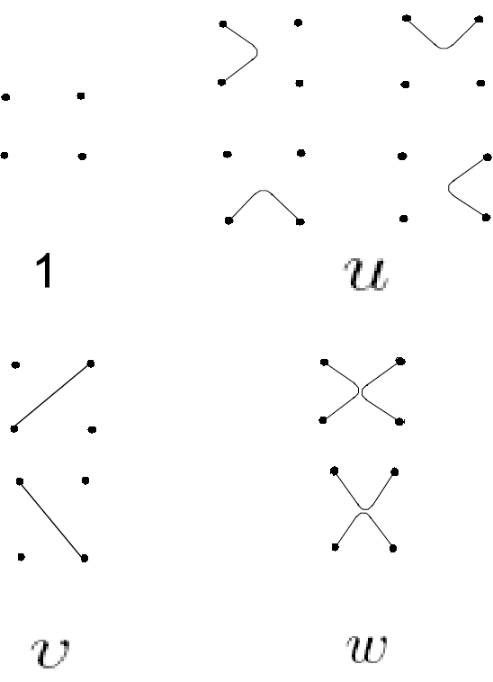
To get the dilute loop models and the loop models corresponding to tri-critical models we need to use Dilute ADE models. These models have rich phase diagrams with four branches: branch 1 and 2 have central charges and branch 3 and 4 have . One can also map this height models to loop models with the non-intersecting bonds on the square lattice with the partition function
| (4.9) |
where the weights for different plaquettes are given in Fig 5 and the and are the numbers of different plaquettes [25]. This generalized loop model apart from the critical properties at and has four other branches coincide with the four branches of dilute ADE models [27]. The weights are given by
| (4.10) | |||||
where , , and are the intervals corresponding to branches 1, 2, 3 and 4 respectively. They coincide with the different branches in the dilute ADE models.
It is interesting to investigate the connection of the above loop model to the SLE. There are different methods to do that here we use the magnetic operator to find the SLE drift. It was shown in [25] by the numerical calculation that the magnetic exponent of the branch 1 and 2 is identified with where
| (4.11) |
and is related to the central charge of the theory by . Its connection to the loop variables comes from the relation derived from the coulomb gas method [25]. The connection of the magnetic exponent to the SLE drift is as follows [26]
| (4.12) |
Using the above equation the SLE drift at the branches 1 and 2 of the loop model (4.9) can be derived as follows
| (4.13) |
This result is consistent also with our expectation from the second level null vector of minimal models [28], it is also consistent with the recent direct investigation by using holomorphic variables [29] .
Back to the height model representation one can summarize following results: the branch 2 of the ADE models corresponds to the dilute loops with and the branch 1 is the dense phase of tri-critical models with . The results for some of the simple cases are as follows:
Using the above method it is easy to find the lattice realization for most of the proposed loop models, the results are interestingly consistent. Following the same method it is possible to extract the loop models corresponding to minimal CFTs, however, the loop model for the non-diagonal cases with is not extractable with this method because we are not able to find the dense phase of loop models for these cases. It seems that the dense lattice height model has not been proposed for this case.
To conclude this subsection we proposed some loop representations
for the minimal CFTs by using fusion of boundary operators. Then
since ADE models give a lattice statistical model representation for
minimal CFTs we used these models to extract physical loop models
corresponding to ADE models. The fractal properties of these lattice
loop models are the same as the loop models that we proposed by
using the fusion of primary operators.
Models: It is possible to follow the same
calculation for every unitary minimal model. For example for WZW
models the classification of modular invariant partition
functions is based on A-D-E-T graphs with . The same method
as the minimal models is applicable here and one can find boundary
operators with . The loop models
have weights . Only has critical
loop representation with the following loop weight
| (4.14) |
with and for the dilute and dense phase respectively. The other loop models are not critical except for with . The fusion graphs of the operators with is not decomposable to the simple graphs, however, the non-largest eigenvalues can be still relevant. For example take with , the fusion graph is similar to the one part of the fusion graph of the tri-critical 3-state Potts model, the right one in fig 6. The eigenvalues are , and , the last two cases have critical loop representation. The similarities between fusion graphs of models with minimal models is not just an accident they are based on the coset construction of the minimal models.
5 Discussion
We proposed a method to classify some possible loop models consistent with the conformal boundary conditions for generic rational CFT: take the simply laced classification of the corresponding minimal CFT then find the boundary operators and also the fusion matrices, make the loop model of the primary operator by the method that we discussed in section 3 and [4]. We think that there should be some connections between these loop models and the SLE interpretation of CFT investigated in [28] which is based on the connection of SLE with the null vectors in the CFT. This connection is not complete even for minimal CFTs because we do not know how to explain the boundary operators with the same loop model but with the different null vectors, for example in the three states Potts model and are in the same sector from the boundary CFT point of view but just and have the required second level null vectors. However, from null vector point of view this correspondence is not clear but it is possible to show that in the partition function level this similarity is more known. Another way to look at the results of this paper is by conjecturing the largest eigenvalue of the fusion graph as the possible loop weight for the loop model in the universality class of the corresponding CFT without defining any height model on the fusion graph.
One possible generalization of the above construction is by
considering graphs with largest eigenvalue bigger than 2 as an
adjacency graph of fused RSOS model and then extracting the loop
model by the method investigated in [16]. The other
interesting direction is to investigate the modular invariant
partition functions of loop models and their possible connections to
the classified modular invariant partition functions of minimal
models, this is related to investigate more directly the connection
of our method to the classification of [5, 6].
Acknowledgment:
I thank Roberto Tateo for useful discussions and Paul Fendley for useful comments. I thank also John Cardy for his useful criticism.
6 Appendix
![[Uncaptioned image]](0808.0100v2/tricriticalpotts.png)
![[Uncaptioned image]](0808.0100v2/tricriticalpotts2.png)
In this appendix we list the fusion graphs of the boundary operators in tri-critical 3-state Potts model. The fusion graphs are given in fig 6. The fusion graph of can be derived from the fusion graph of the operator by the following transformations:
| (6.15) |
The fusion graph of can be derived from the fusion graph of the operator by the following transformations:
| (6.16) |
Finally the fusion graph of can be derived from the fusion graph of the operator by the following transformations:
| (6.17) |
To get the fusion graphs of and from the fusion graph of one just need to use the transformations (6.16) and (6.17) respectively.
We shall call the part of the fusion graph of with two neighbor blobs , the lower index is the number of nodes and the upper index is the number of blobs attached to the neighboring nodes of the graphs starting from one of the extremes. These kinds of fusion graphs appear also in the fusion graph of of models.
References
- [1] B. Nienhuis, Journal of Statistical Physics, Vol.34, Nos.5/6(1984)
- [2] M. Freedmann, Comm. Math. Phys. 234, 129 (2003)[quant-ph/0110060], M. Freemann, C. Nayak and K. Shetengel, Phys. Rev. Lett.94, 147205 (2005)[cond-mat/0408257]
- [3] O. Schramm, Israel J. Math. 118, 221, 2000[math. PR/9904022]
- [4] M. A. Rajabpour, J. Phys. A 41:405001, 2008 [arXiv:0806.4520]
- [5] J. L. Jacobsen, H. Saleur, Nucl.Phys.B788:137-166,2008 [math-ph/0611078]
- [6] J. Dubail, J. L. Jacobsen, H. Saleur[0812.2746 ]
- [7] J. Cardy, J. Stat. Phys. 125, 1 (2006); cond-mat/0604043.
- [8] A. Cappelli, C. Itzykson and J.-B. Zuber, Comm. Math. Phys. 113, 1 (1987).
- [9] G. E. Andrews, R. J. Baxter and P. J. Forrester, J. Stat. Phys. 35, 193 (1984); P. J. Forrester and R. J. Baxter, J. Stat. Phys. 38, 435 (1985); V. Pasquier, Nucl. Phys. B285, 162 (1987).
- [10] P. Roche, Phys. Lett. B 285 (1992) 49-53
- [11] S. O. Warnaar and B. Nienhuis, J.Phys. A26 (1993) 2301-2316
- [12] J. L. Cardy, Nucl. Phys. B324, 581 (1989).
- [13] R. E. Behrend, P. A. Pearce, J. B. Zuber; J.Phys. A31 (1998) L763-L770; R. Behrend, P. Pearce, V. Petkova, J.-B. Zuber; Phys.Lett. B444 (1998) 163-166
- [14] R. Behrend, P. Pearce, V. Petkova, J.-B. Zuber; Nucl.Phys. B570 (2000) 525-589; Nucl.Phys. B579 (2000) 707-773
- [15] B. Nienhuis, Phys. Rev. Lett. 49, 1062 - 1065 (1982)
- [16] P. Fendley, J.Phys. A39 (2006) 15445[cond-mat/0609435 ]
- [17] P. Fendley, J. L. Jacobsen, J. Phys. A: Math. Theor. 41 (2008) 215001 [arXiv:0803.2618]
- [18] L. Chim, Int. J. Mod. Phys. A11 (1996) 4491[hep-th/9510008]; R. I. Nepomechie, J.Phys. A34 (2001) 6509-6524 [hep-th/0102010]
- [19] P. Fendley and P. Ginsparg, Nuclear Physics B 324,(1989)549-580
- [20] Y. Deng, H. W. J. Blöte and B. Nienhuis; Phys. Rev. E 69, 026123 (2004)
- [21] Y. Deng, W. Guo and H. W. J. Blöte; Phys. Rev. E 72, 016101 (2005)
- [22] I. Affleck, M. Oshikawa, H. Saleur; Journal of Physics A: Mathematical and General, Volume 31, Issue 28, pp. 5827-5842 (1998) [cond-mat/9804117]
- [23] A. Gamsa, J. Cardy, J. Stat. Mech. (2007) P08020[arXiv:0705.1510 ]
- [24] J. Cardy, J.Phys. A40 (2007) 1427-1438[math-ph/0610030 ]
- [25] H. W. J. Blöte and B. Nienhuis, Journal of Physics A: Mathematical and General, Volume 22, Issue 9, pp. 1415-1438 (1989)
- [26] O. Schramm, S. Sheffield, D. B. Wilson, [arXiv:math/0611687]
- [27] S. O. Warnaar, B. Nienhuis, and K. A. Seaton, Phys. Rev. Lett. 69, 710 - 712 (1992)
- [28] M. Bauer, D. Bernard, Phys.Lett. B543 (2002) 135-138 [math-ph/0206028], R. Friedrich, W. Werner, Comptes Rendus Mathematique, 335, 11, 2002, 947-952[math/0209382], E. Bettelheim, I. A. Gruzberg, A. W. W. Ludwig, P. Wiegmann, Phys. Rev. Lett. 95 (2005) 251601 [hep-th/0503013]
- [29] Y. Ikhlef, J. Cardy, J. Phys. A: Math. Theor. 42 (2009) 102001 [arXiv:0810.5037 ]