Optimal weighting in constraints from large scale structure in an idealised case
Abstract
We consider the problem of optimal weighting of tracers of structure for the purpose of constraining the non-Gaussianity parameter . We work within the Fisher matrix formalism expanded around fiducial model with and make several simplifying assumptions. By slicing a general sample into infinitely many samples with different biases, we derive the analytic expression for the relevant Fisher matrix element. We next consider weighting schemes that construct two effective samples from a single sample of tracers with a continuously varying bias. We show that a particularly simple ansatz for weighting functions can recover all information about in the initial sample that is recoverable using a given bias observable and that simple division into two equal samples is considerably suboptimal when sampling of modes is good, but only marginally suboptimal in the limit where Poisson errors dominate.
pacs
98.80.Jk, 98.80.CqI Introduction
The currently most attractive theory for the emergence of structure in the Universe is inflation [1, 2, 3, 4]. It is generically successful at diluting the primordial defects to undetectable densities and predicts a nearly-flat universe with nearly scale invariant spectrum of primordial fluctuations that are normally distributed and extend to scales larger than horizon [5, 6, 7, 8, 9]. To understand details of the inflation, on must look at detailed predictions of different models. Non-Gaussianity of the primordial curvature perturbations, i.e small departures from the normal distribution of fluctuations is one aspect in which models of inflation differ.
Recently, non-Gaussianity of the local type has received a renewed attention. This type of non-Gaussianity is characterised by a quadratic correction to the potential [10, 11, 12, 13]:
| (1) |
where is the primordial potential assumed to be a Gaussian random field and describes the amplitude of the correction during the matter domination era. There are two main reasons for this renewed interest. First, there is a hint of a detection in the cosmic microwave data [14] and several non-detections [15, 16, 17]. Second, a new method for its detection has been recently proposed in [18]. This method uses biased tracers of structure for which it can be shown that local-type of non-Gaussianity leads to a very particular scale-dependence of the bias
| (2) |
where is the bias induced by non-Gaussianity, is the tracer’s intrinsic bias and is given by
| (3) |
where is the matter transfer function normalised to unity at , is the growth function normalised to in the matter era, is the linear over-density at collapse for the spherical collapse model and other symbols have their usual meaning. Note that becomes significant only at large scales, where non-linearities and scale-dependent bias are expected to be small and therefore offers a surprisingly clean probe of non-Gaussianity. This equation has been re-derived, scrutinised and better understood in the subsequent work [19, 20, 21, 22].
A first application of this method to the real data using a wide variety of tracers of large scale has recently shown the promise of this method [20, 21]. The derived constraints are already competitive with those coming from the cosmic microwave background. In that work, the constraints were derived by comparing the power spectrum of the distribution of tracers with those predicted by the theory. At largest scales, where the effect coming from the non-Gaussianity is the largest, the method suffers from the sample variance. In other words, the finite number of large-scale modes in any survey severely limits our ability to measure the power spectrum. Recently, Seljak has suggested a method of circumventing this limitation [23]. This method essentially considers two differently biased tracers that sample the same volume. The ratio of amplitudes of a single mode for the two tracers will give the ratio of the two biases , but the amplitude of the primordial mode cancels out. One thus measures the auto correlation power spectra of the two tracers in the same volume. By taking the ratio of these two spectra, one can put a constraint on the value of , which is independent on the primordial field and thus unaffected by the sample variance. The biases and can be derived from the amplitude of small scale fluctuations, where sampling variance is not a problem and hence, one extremely well measured large-scale mode is in principle enough to constrain . A more robust technique would be to assume nothing about the matter power spectrum and derive limits on from limits on the scale dependence of ratio of . This would protect measurements of from systematics arising from, for example, massive neutrinos.
In practice, one rarely has two distinct samples with a well-defined bias. In this work, we extended the analysis by considering a single tracer of the underlying field that spans a range of biases and attempt to answer the question of how to optimally analyse such tracer. The approach we take is to create two effective samples and to optimally weight the tracer’s constituents.
II Approach and limitations of this work
In this paper we assume that the Equations (2) and (3) are exactly correct. These equations have initially been derived using Press-Schecter[24] and related formalisms. They have now been tested for dark matter halos against -body simulations in two publications [25, 26] with somewhat differing conclusions. This is an issue that will have to be settled before further measurements of are possible.
If luminous objects are used for constraining the parameter, they must sample the underlying population of halos randomly in the sense that they must insensitive to any property of the halo that might be correlated with the large-scale modes that induce the dependence. While this is true for most objects, it is not necessarily true for quasars as discussed in [27], where the Equation (2) was generalised to with for random halos and for a population that is hosted by the recently merged halos. This is, of course, a rather crude approximation, but it illustrates a possible violation of the Equations (2) and (3).
If this assumption holds then the stochasticity of each tracer will be zero on scales much larger than the typical halo size. Stochasticity is a measure of how well a given tracer of large scale structure samples the underlying dark matter field in the Gaussian cosmologies. In this work we consider a single tracer whose constituents have a range of biases and zero stochasticity. In particular, each galaxy (or quasar or some other tracer) has an associated bias , so that a subset of galaxies whose biases lie between and is a perfect tracer of the underlying dark matter field with a constant bias . In other words, in Fourier space on scales of interest,
| (4) |
where is the over-density of galaxies and is the over-density of matter at some wave-vector . This assumption can be checked by considering the quantity , where is the cross-correlation power spectrum for the two samples and / are the corresponding auto-correlation power spectra. Recent cross-correlation studies using counts in cells have shown that on large scales ( Mpc) the stochasticity is indeed very small [28]. It is not fundamental limit, but it means that improvement in signal to noise will stop beyond [23], where is the cross-correlation coefficient. It is also possible the clever schemes around this limitation might be constructed [29].
Moreover, we assume that the noise associated with the sparse sampling of the underlying field can be described by a Poisson statistics. While this sounds a very reasonable approximation, recent work on -body simulations indicate that the actual shot noise properties might significantly deviate from Poisson statistics11 1 Uroš Seljak, private communication..
Next we assume that there exist an observable that can be thought of as a proxy for the individual galaxy’s bias. In practice, this can be the galaxy’s luminosity, but in this paper we often operate with host halo bias mass that allows us to connect our calculations with the standard mass functions of the halo model. Since the bias is an ill-defined quantity on a single object, it suffices that an ensemble of galaxies with luminosity between and has a mean bias . If is a “noisy” estimator for the galaxy’s bias then the range of biases obtainable from various slicing of the original sample will be limited and hence any weighting based on will be suboptimal. In the limiting case when is a completely random variable, any slicing would produce two samples of the same bias and therefore it is impossible to put limits on using method of [23]. Our work derives the optimal weighting within the possibilities offered by a given measurable quantity and not optimal weighting in an absolute sense.
The purposed of this paper is to derive the optimal weighting subject to limitations described above. However, it must be stressed that if these conditions are not satisfied, the weighting will be suboptimal, but it would not lead to biased results. This is equivalent to the inverse covariance weighting used in optimal quadratic estimators (see e.g. [30]). If wrong power spectrum is used to create the covariance matrix, or if no inverse covariance weighting is performed at all, the results are suboptimal and the error-bars are larger then necessary, but results are not biased. Situation here is similar: the method that we present here is trivial to implement on real data, while the truly optimal weighting would require massive numerical work. We therefore deem it a useful step towards decreasing the error-bars on constraints in future observational work.
The paper is organised as follows. In Section III, we consider slicing the sample into infinitely thin subsamples of varying bias and derive an analytic expression for the maximum signal-to-noise that can be obtained using a Fisher matrix analysis. In the subsequent Section IV we consider how the sample can be weighted using two weighting functions to get two effective samples. We construct a weighting method whose Fisher matrix element for is the same as those of the optimal analysis and is thus itself optimal. We show that simple methods of dividing the sample into two can be considerably ineffective. Section V briefly compares our results with optimal weights used in power spectrum determination. Final thoughts can be found in the Conclusions.
III Information content in a tracer
Consider a tracer of mass that is composed of many individual objects that have different biases with respect to the underlying density field. For simplicity, let us assume that the variable that determines an individual object’s bias is its host halo mass, but note that in general it can be any continuous variable that varies monotonically with bias. The population is then characterised by , the average bias of the objects with mass and the mass function , which is the number density of objects with mass between and . Let slice the total number of objects into samples of different average bias. Each slice is centred around mass , where and has bias with number density of . Following [23], we consider one Fourier mode of the underlying density field. Its covariance matrix has the form
| (5) |
Our ability to constrain is determined by the Fisher matrix, whose elements are
| (6) |
evaluated at our fiducial model, which has . In that limit we have
| (7) | |||
| (8) |
In Appendix A we show that the inverse of is given by
| (9) |
where we have replaced sums with the integrals and defined averages to be over the mass function:
| (10) | |||
| (11) | |||
| (12) |
After some cumbersome, but straight-forward algebra, we arrive at
| (13) |
where
| (14) |
and
| (15) | |||
| (16) | |||
| (17) |
This result encodes that maximum information that can be extracted from a sample of objects.
To get a better intuition about this formula, we define
| (18) |
In the Figure 1 we plot the functional shape for a couple of values of , and .
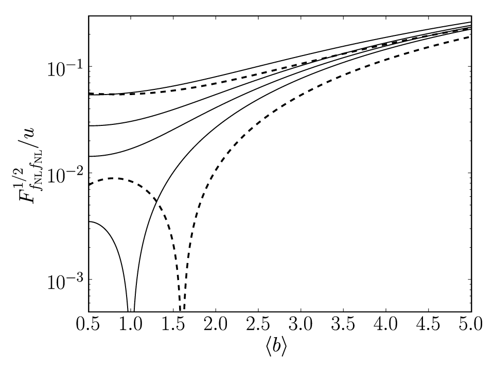
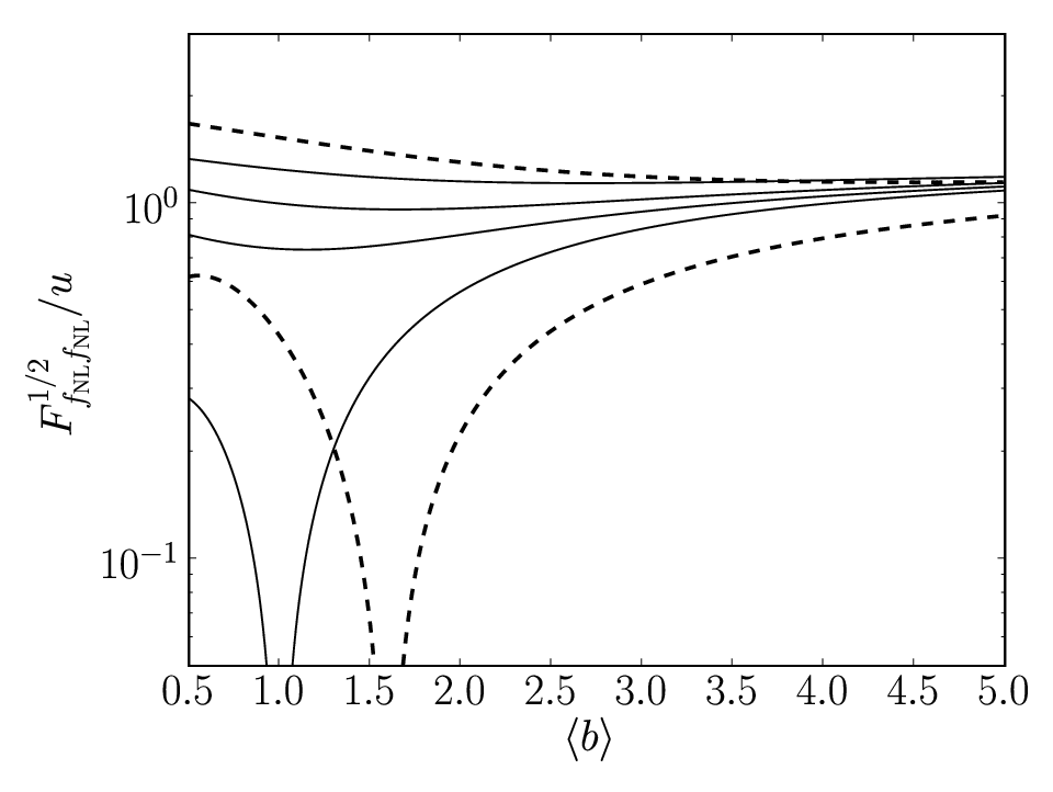
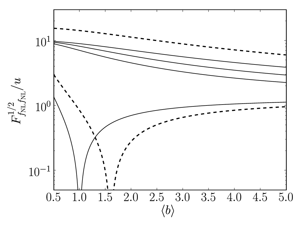
This figure deserves some discussion. As expected in the limit of , the signal to noise drops to zero at and monotonically increases with bias. In general, however, this is not the case. When we are in the Poisson limit and sampling is sparse, then it is still better to go with objects with the highest bias. In the other limit, when sampling of the modes is very good, it is better to have a bigger relative spread in the bias rather than bias that is high in average. This is slightly counter-intuitive, but remember that we assume here that each object has a known bias. But most importantly, when the overall best signal to noise is roughly independent of the mean bias, as long as we cover a sizeable range of biases.
This analysis corresponds to a single mode. For any realistic survey, one needs to integrate across observed modes. The final error on is given by
| (19) |
where is the volume of the survey and the pre-factors come from the volume of a single mode in the -space which equals .
The result of the Equation (13) is the maximum information that is in principle available for extraction. In practice, it is not clear, how to extract this information - it would require a very fine slicing by the bias with cross-correlation of each slice with every other slice. In the next section we attempt a different approach - we divide the sample into two different samples and adjusts the weighting of the objects in the two samples so that the signal is maximised.
IV Optimal weighting
Following the previous section, we will consider weights that are function of the halo mass . In practice, we do not know the host halo mass for individual objects, but one can equivalently use any proxy for bias, such as luminosity.
Let us therefore consider two weighting functions and . Any given object in the sample counts as objects. For example, when calculating the over-density in a cell, we weight the objects by :
| (20) |
where index runs over the halos in a given cell of volume and the mean weighted object density is given by
| (21) |
and the same for the sample.
Using properties of the Poisson statistics, the effective bias and corresponding Poisson error are given by
| (22) | |||
| (23) |
and an equivalent expression for the sample. An important subtlety is, that if the weighting functions overlap, the cross term also acquires a Poisson error, given by
| (24) |
For a two-sample case, the final error on the can therefore be calculated by combining Equations (5) (with new Poisson errors in the cross term), (6) and (19). Note that results are independent of any multiplicative constant on or . However, one cannot assume that we are in the Poisson limit and therefore the matrix inversions have to be done without approximations. However, since we are discussing matrices, this is not impossible.
Consider next the following form for weighting functions and :
| (25) | |||
| (26) |
In this case, the relevant variables simplify to:
| (27) | |||
| (28) | |||
| (29) | |||
| (30) | |||
| (31) | |||
| (32) | |||
| (33) |
We can now combine Equations (27) – (33) with Equations (5) and (6) to obtain expression for . This is a very cumbersome process that is best done with the help of a mathematical computer package. The final result, however reduces to the exactly the same expression as that of Equation (13). This is a very interesting result. It shows that any weighting that has the form of Equations (25) – (26) produces optimal sensitivity to the .
In order to avoid dealing with nearly singular matrices, it is in practice advantageous to have weighting functions that have as little overlap as possible. We therefore propose the following form the weighting functions:
| (34) | |||
| (35) |
where and are the minimum and the maximum value of bias in the range of interest. These optimal weighting functions are the main result of this paper.
How does this compare to other weighting functions? The simplest case would be to divide the sample into two disjoint samples with no overlap:
| (36) | |||
| (37) |
where is the Heaviside step function and the barrier mass is a free parameter. This is essentially equivalent to the analysis of [23], where presumably an absolute magnitude cut is proposed to create two samples of a different bias.
We choose two possible values for . First we consider such that the integral is the same for both samples. Second we use the that is such as to minimise the overall .

In Figure 2 we plot how close the error on approaches the theoretically minimal error obtained by optimal weighting. To plot this figure, we have assumed a fiducial flat CDM cosmology with matter density , spectral index of primordial fluctuations of and normalisation in 8 Mpc/ spheres of . Moreover, we assumed a survey centred at redshift with volume and tracers with and used the mass function from the Sheth-Tormen theory and bias from an extended Press-Schecter formalism [31, 32]. The upper limit of integration was set to Mpc/.
The x-axis of the plot is the minimal mass used for calculation of and . The upper set of lines corresponds to a naive ansatz of making equal for both subsamples, while the bottom set of lines for the best possible division that can be obtained using two disjoint samples with no weighing. The dashed and dotted lines show the dependence on the number-density of objects. Note, that changing the number density affects both optimal as well as suboptimal weighting and that we plot just the ratio of the two error-bars, rather than the size of the error-bars themselves.
We see that the closer one is to the limit of well-sampled modes the more important it is to use weighting, but that weighting does not make any difference in the Poisson-limited sampling. For the particular survey parameter that we chose, we note that for set by equal for both samples, the weighting function can be suboptimal to up to a factor of in the limit of small , but that even the numerically optimised can be significantly suboptimal.
The above results have to be take with a pinch of salt, since we have used bias dependence on mass and the corresponding mass function rather than bias dependence on luminosity and the luminosity function . The latter is more closely related to the observations. Due to the scatter in luminosity – bias relation, the range of biases available by weighting by b(L) is smaller and this will affect the results.
V Comparison with power spectrum weighting.
Interestingly, the equations present in this paper are very close to those that can be found in [33]. In that work, authors find the optimal weighting for power spectrum determination for a continuously biased tracer by generalising Feldman, Kaiser & Peacock [34] approach. In fact, the equations are very similar. Following exactly the same procedure as in Section III, but for the power spectrum rather than , one gets that in the limit of infinitely thin slicing
| (38) |
By using the weighing function 22 2 We note that multiplicative factors on weighting function do not enter into the Fisher matrix analysis. One must nevertheless get them right to form an unbiased estimator., which is the optimal weighting function found in [33] in our notation, we can show that a single sample weighted with (i.e, the one-dimensional covariance matrix) again recovers the full information . We therefore independently confirm the results of [33].
It is important to note that in this work, we have optimised for a maximal rather than a minimal . In other words, we calculate the weighting that maximises our ability to constrain , assuming that other parameters, such as are fixed and are presumably constrained from other probes, such as cosmic microwave background.
VI Conclusions
In this paper we have analysed the problem of optimal weighting of biased tracers of structure with the goal of extracting maximum information about the non-Gaussianity parameter . We have derived the minimum error on by considering slices that are infinitely thin in bias. We have shown that a simple weighting scheme of Equations (25) and (26) obtains the same constraining power. General division of the full sample into two subsamples can be considerably sub-optimal even when mass at which the samples are divided is carefully chosen.
The optimal weighting scheme of Equations (25) and (26) is surprisingly simple. In fact, the product does not come into weighting at all - this is a lucky coincidence, which allows us to use the same optimal weighting for every mode, rather to optimize weighting around some fiducial wave-vector.
The result in this paper is subject to the assumptions outlined in the Section II of this paper. If these assumptions are violated, the weighing is sub-optimal, but probably nevertheless beneficiary. Since any division into two samples by e.g. an absolute magnitude cut requires some knowledge of bias, the implementation of the scheme proposed in this paper is likely to be very simple.
How can this be put in practice? In this work we have used halo mass as a proxy for the bias. However, our analysis is completely general and one can replace the host halo mass with any variable that is monotonically linked to the bias. For example, one could take luminous red galaxies (LRGs) and determine their bias by splitting the entire sample into several subsamples in different luminosity bins and the constrain a smooth function , which describes the variation of galaxy bias with its luminosity, using modes which are not affected by the . One would next construct two effective samples by optimally weighting the original sample using Equations (25) and (26) and replacing with . In the next step, auto and cross-correlation power spectra of these two samples should be calculated, taking into account the Poisson error correlation between the two. At this step, one can use the cross-correlation spectra to check for the amount of stochasticity, which has been assumed to be negligible in this work. Finally, should be constrained using these power spectra as input.
Acknowledgements
Numerical codes used in preparation of this paper used the mass functions prepared using code by Darren Reed [35]. Author thanks Will Percival for pointing out analogies with optimal weighting of biased tracers for power spectrum estimation and acknowledges useful discussions with Uroš Seljak. This work is supported by the inaugural BCCP Fellowship.
Appendix A Inversion of matrix
We can rewrite Equation (7) as
| (39) |
where , is the identity matrix and . The inverse of can then formally be written as an infinite series
| (40) |
We note that the product
| (41) |
and so we can rewrite the inverse of as
| (42) |
Since is diagonal and hence trivial to invert, the Equation (40) simplifies to
| (43) |
References
- [1] A. A. Starobinsky, JETP Lett. 30, 682 (1979).
- [2] A. H. Guth, Phys. Rev. D 23, 347 (1981), ADS.
- [3] A. Linde, Physics Letters B 108, 389 (1982).
- [4] A. Albrecht and P. J. Steinhardt, Phys. Rev. Lett. 48, 1220 (1982), ADS.
- [5] V. F. Mukhanov and G. V. Chibisov, Journal of Experimental and Theoretical Physics Letteres 33, 532 (1981), ADS.
- [6] S. W. Hawking, Physics Letters B 115, 295 (1982), ADS.
- [7] A. H. Guth and S.-Y. Pi, Phys. Rev. Lett. 49, 1110 (1982), ADS.
- [8] A. A. Starobinsky, Physics Letters B 117, 175 (1982), ADS.
- [9] J. M. Bardeen, P. J. Steinhardt, and M. S. Turner, Phys. Rev. D 28, 679 (1983), ADS.
- [10] D. S. Salopek and J. R. Bond, Phys. Rev. D 42, 3936 (1990), ADS.
- [11] A. Gangui, F. Lucchin, S. Matarrese, and S. Mollerach, Astrophys. J. 430, 447 (1994), arXiv:astro-ph/9312033.
- [12] L. Verde, L. Wang, A. F. Heavens, and M. Kamionkowski, Mon. Not. R. Astron. Soc. 313, 141 (2000), arXiv:astro-ph/9906301.
- [13] E. Komatsu and D. N. Spergel, Phys. Rev. D 63, 063002 (2001), arXiv:astro-ph/0005036.
- [14] A. P. S. Yadav and B. D. Wandelt, Phys. Rev. Lett. 100, 181301 (2008), arXiv:0712.1148.
- [15] P. Creminelli, L. Senatore, M. Zaldarriaga, and M. Tegmark, Journal of Cosmology and Astro-Particle Physics 3, 5 (2007), arXiv:astro-ph/0610600.
- [16] E. Komatsu, J. Dunkley, M. R. Nolta, C. L. Bennett, B. Gold, G. Hinshaw, N. Jarosik, D. Larson, M. Limon, L. Page, et al., ArXiv e-prints 803 (2008), arXiv:0803.0547.
- [17] C. Hikage, T. Matsubara, P. Coles, M. Liguori, F. K. Hansen, and S. Matarrese, ArXiv e-prints 802 (2008), arXiv:0802.3677.
- [18] N. Dalal, O. Doré, D. Huterer, and A. Shirokov, Phys. Rev. D 77, 123514 (2008), arXiv:0710.4560.
- [19] S. Matarrese and L. Verde, Astrophys. J. Lett. 677, L77 (2008), arXiv:0801.4826.
- [20] A. Slosar, C. Hirata, U. Seljak, S. Ho, and N. Padmanabhan, ArXiv e-prints 805 (2008a), arXiv:0805.3580.
- [21] N. Afshordi and A. J. Tolley, ArXiv e-prints 806 (2008), arXiv:0806.1046.
- [22] P. McDonald, ArXiv e-prints 806 (2008), arXiv:0806.1061.
- [23] U. Seljak, ArXiv e-prints 807 (2008), arXiv:0807.1770.
- [24] W. H. Press and P. Schechter, Astrophys. J. 187, 425 (1974), ADS.
- [25] V. Desjacques, U. Seljak, and I. T. Iliev, ArXiv e-prints (2008), arXiv:0811.2748.
- [26] A. Pillepich, C. Porciani, and O. Hahn, ArXiv e-prints (2008), arXiv:0811.4176.
- [27] A. Slosar, C. Hirata, U. Seljak, S. Ho, and N. Padmanabhan, Journal of Cosmology and Astro-Particle Physics 8, 31 (2008b), arXiv:0805.3580.
- [28] M. E. C. Swanson, M. Tegmark, M. Blanton, and I. Zehavi, MNRAS 385, 1635 (2008), arXiv:astro-ph/0702584.
- [29] S. Bonoli and U.-L. Pen, ArXiv e-prints (2008), arXiv:0810.0273.
- [30] M. Tegmark, Phys. Rev. D 55, 5895 (1997), ADS.
- [31] R. K. Sheth and G. Tormen, Mon. Not. R. Astron. Soc. 308, 119 (1999), arXiv:astro-ph/9901122.
- [32] R. K. Sheth, H. J. Mo, and G. Tormen, Mon. Not. R. Astron. Soc. 323, 1 (2001), ADS.
- [33] W. J. Percival, L. Verde, and J. A. Peacock, Mon. Not. R. Astron. Soc. 347, 645 (2004), arXiv:astro-ph/0306511.
- [34] H. A. Feldman, N. Kaiser, and J. A. Peacock, Astrophys. J. 426, 23 (1994), arXiv:astro-ph/9304022.
- [35] D. Reed, R. Bower, C. Frenk, A. Jenkins, and T. Theuns, MNRAS 374, 2 (2007), arXiv:astro-ph/0607150.