On quark masses in holographic QCD
Abstract:
Recently certain nonlocal operators were proposed to provide quark masses for the holographic model of QCD developed by Sakai and Sugimoto. The properties of these operators at strong coupling are examined in detail using holographic techniques. We find the renormalization procedure for these operators is modified by the running of the five-dimensional gauge coupling. We explicitly evaluate the chiral condensate characterized by these operators.
Keywords:
D-branes, Supersymmetry and Duality, Brane Dynamics in Gauge Theories1 Introduction
Gauge/gravity dualities have proven to be a remarkable new framework to study a large class of strongly coupled gauge theories [1, 2]. However, the gauge theories that are currently amenable to such holographic analysis are typically very different from real world QCD. Hence constructing a holographic model of QCD remains one of the most important challenges for this approach. Currently, the most successful proposal is a construction by Sakai and Sugimoto [3, 4] based on a configuration of D8- and -branes in a D4-brane background. While reliable calculations are limited to large and small , many observables seem to show a good approximation to real QCD at low energies.
A key feature of the Sakai-Sugimoto model is that it exhibits the desired non-Abelian chiral symmetry , as well as its spontaneous breaking [3, 4]. Of course, in real world QCD, the analogous symmetry is only approximate as it is explicitly broken by the quark masses. A shortcoming of the D8//D4 model then is that the quarks are precisely massless. While various suggestions have been made to introduce quark masses [5, 6, 7, 8, 9], there remain technical difficulties in pursuing these proposals in detail. A recent proposal which seems easier to study is based on deforming the model with certain nonlocal operators [10, 11, 12]. The underlying microscopic field theory is a five-dimensional gauge theory where the chiral quarks are localized on separate four-dimensional defects. Since the fermions of different chiralities are separated in the five-dimensional spacetime, no simple local mass term can be introduced in the UV field theory. However, this spatial separation can be overcome by connecting two quark fields with a Wilson line. Hence a natural suggestion is to introduce a nonlocal operator to provide a quark mass deformation [10, 11, 12]:
| (1) |
As has been extensively studied for closed Wilson lines [13, 14], such a nonlocal operator would be dual to an instantonic string worldsheet which extends between the D8- pair. In the following, we examine the properties of these operators in some detail.
An overview of the paper is as follows: in section 2, we review the construction of the Sakai-Sugimoto background. In section 3, we consider the nonlocal mass terms introduced in [10, 11]. In particular, we examine the affect of the dilaton coupling to the string worldsheet. Even though this coupling only appears at higher order in the expansion, we find that in the D4-brane background it introduces a interesting modification in the renormalization of the Wilson line. In section 4, we explicitly calculate the expectation value of these nonlocal operators. In the absence of any local fermion bilinears, this expectation value or condensate is an order parameter characterizing the chiral symmetry breaking in this holographic model. We close in section 5 with a discussion of our results and by making a few observations about future directions. Appendix A provides the details of a calculation of the fluctuation determinant of the worldsheet fields. The latter contributes at the same order as the dilaton coupling but does not make any further modifications of the renormalization of the nonlocal operators.
2 Review of Sakai-Sugimoto background
The Sakai-Sugimoto model [3, 4] is based on the throat limit of intersecting D4- and D8-branes, summarized by the array
| (2) |
The world-volume theory of the D4-branes naturally gives rise to a maximally supersymmetric gauge theory in five dimensions. Following [15], the direction is compactified and antiperiodic boundary conditions are imposed on the fermionic fields around this circle. In the far infrared, one might expect that the only relevant degrees of freedom arising from this D4 world-volume theory correspond to four-dimensional Yang-Mills with gauge group . Further the intersection of the D4-branes with D8-branes supports chiral fermions in the fundamental representations of the gauge group and of the flavour symmetry. These fermions propagate in the dimensions common to both sets of branes. Similarly, the intersection with -branes produces an analogous set of four-dimensional anti-chiral fermions. Hence, the Sakai-Sugimoto model produces a holographic description of QCD in the throat limit of the D4-branes. The dual gravity theory in this framework yields reliable results for large and strong ’t Hooft coupling. Our current understanding of this holographic model is limited to the quenched approximation, i.e., , in which the D8-branes are probes in the supergravity background.
2.1 D4-brane background
Here we review the supergravity background, which we refer to as the the D4 soliton (following the nomenclature of [16]). This throat geometry for a stack of D4-branes with antiperiodic fermions on the circle is the gravitational dual of a confined phase of the gauge theory [15], as described above. For comparison purposes, we also consider the supersymmetric D4-brane throat with fermions that are periodic on the circle. Both solutions can be expressed in the form 11 1 The normalization for is different from what is prevalent in the literature and has been chosen to be consistent with the usual IIA action,
| (3) | |||
| (4) |
The four noncompact directions of the gauge theory correspond to and with , while the coordinate labels the compact direction. The 56789-directions transverse to the D4-branes are described by a radial coordinate and four angles that parameterize a unit four-sphere. The -invariant line element on this sphere is , and the volume form is . The function is given by
| (5) |
but the constant for the supersymmetric background.
The D4 soliton appears to have a conical singularity at . Regularity requires that the period of the compact direction, , is given by
| (6) |
With this choice the circle smoothly shrinks to zero size at . Fermionic fields in the bulk must be antiperiodic on this circle, reflecting the antiperiodic boundary condition on fermions in the dual gauge theory. Unlike the soliton background, the supersymmetric D4-brane geometry with exhibits a naked curvature singularity at . In that case there is no restriction on the periodicity of the direction. Further, the dual gauge theory is not confining.
The supergravity solution described above is completely specified by the string coupling constant, , the RR flux quantum (i.e., the number of D4-branes), , and the non-extremality constant, . The remaining parameter is a length scale, , which is given in terms of these quantities and the string length, , by
| (7) |
Various combinations of these parameters have direct interpretations in the dual gauge theory. The holographic dictionary gives the five-dimensional gauge coupling as , so that the five-dimensional ’t Hooft coupling is
| (8) |
Since these couplings have dimensions of length there is a power-law running of the dimensionless effective coupling [17]
| (9) |
where the energy scale is related to the radial coordinate in the D4-brane throat by [18]. One finds that the scale of Kaluza-Klein excitations of the compactified coordinate gives the characteristic mass for glueballs [19]
| (10) |
Below this scale, the low-energy gauge coupling in four dimensions is .
Supergravity provides a good description of physics in the D4-brane background if two conditions are met. First, gravity calculations are reliable if the length scale associated with spacetime curvatures is small compared to the fundamental string tension. In the D4 soliton solution (5) the Ricci scalar has a maximum at , where curvatures are of order . Hence we require
| (11) |
In terms of gauge theory quantities this can be expressed as the condition
| (12) |
so that the restriction to small curvatures corresponds to a large ’t Hooft coupling in the effective four-dimensional gauge theory. Second, string loop effects are suppressed as long as the local string coupling is small: . The form of the dilaton (4) implies that, for finite values of the gauge theory parameters, the inequality can only be satisfied over some finite range of the coordinate . The string coupling eventually becomes at a value of given by
| (13) |
This critical radius naturally becomes large in the limit . Taken together, equations (11) and (13) indicate that the supergravity analysis in the D4-soliton background is reliable in precisely the strong-coupling regime of the ’t Hooft limit of the four-dimensional gauge theory.
In the strong coupling regime the QCD scale cannot be decoupled from the compactification scale, e.g., in the confining phase described by the D4 soliton, the QCD string tension is [15, 20]. This means that, for most practical purposes, calculations in the holographic framework are reliable in a regime corresponding to a five-dimensional gauge theory. Since this theory is nonrenormalizable it should be thought of as being defined with a cut-off scale, . Above this scale a UV completion with new degrees of freedom is required. This completion may be a lift to M-theory, with the circle opening up to reveal an asymptotically AdS background (with identifications). On the field theory side of the duality, the UV completion of the five-dimensional Yang-Mills theory is given by the six-dimensional theory compactified on a circle. An alternative UV completion would simply be type IIA superstring theory in the asymptotically flat D4-brane background.
2.2 D8-brane embeddings
Our current understanding of the holographic model described in the previous section is largely limited to the quenched approximation: . In this limit the D8-branes can be treated as probes embedded in the supergravity background generated by the D4-branes 22 2 See [21], for attempts to account for the gravitational back-reaction of the D8-branes.. The D8-brane fills the noncompact 0123 directions as well as the angles on the transverse to the D4-branes. The nontrivial aspect of the embedding is given by a function that characterizes the D8-brane’s profile in the - plane. With this choice of embedding, the action for the D8-branes is
| (14) |
The resulting equation of motion for is
| (15) |
The expression within the parentheses is constant. If we assume that the profile is symmetric across the -axis, crosses this axis at some value , and is smooth in the vicinity of this point, then this constant is given by . The embedding equation can then be expressed as
| (16) |
The boundary conditions for the D8-brane profile are: asymptotically as , and ; at the minimum , and . The full embedding consists of two halves of this form. Hence the D8- and -branes are joined in a smooth profile at the minimum radius and the two defects are separated by the asymptotic distance in the direction. The limit yields the trivial embedding =constant, which in the D4 soliton background corresponds to a smooth joining of the D8- and -branes with asymptotic separation . In the supersymmetric background () the trivial embedding is also allowed with an arbitrary separation . In this case, the D8- and -branes terminate on the singularity at .
We can gain some intuition for these embeddings by considering the supersymmetric background. In this case with , and hence the embedding equation reduces to
| (17) |
Integrating gives a solution in terms of an incomplete Beta function [22]
| (18) |
This has a finite limit, so that the asymptotic (coordinate) separation of the pair is given by
| (19) |
where . Of course, corresponds to the separation of the defects in the dual gauge theory. With the D4 soliton background there is a maximum separation corresponding to defects located at antipodes on the circle. In the supersymmetric background the coordinate need not be compact, so there is no restriction of this sort. However, other considerations bound the maximum value of which one might consider in this case. Notice that increasing corresponds to smaller values of . If becomes too small, the D8-brane extends into a region of high curvature and the calculation described above is no longer reliable. Therefore one can only reliably work with values of where the minimum of the brane embedding is safely outside of this region.
With periodic fermions, the adjoint sector of the theory is supersymmetric and the gauge theory is not confining. In the dual background, free “constituent” quarks are realized as strings stretching from , the minimal radius of the branes, down to . The energy of these strings corresponds to the mass of the constituent quarks: . With (19), this dynamically generated mass scale is given by
| (20) |
Since we always have in the strong coupling regime, which reflects the fact that the infrared dynamics does not decouple from the compactification scale. In the confining background of the D4 soliton background, there are no free quarks but one can still show that has the interpretation of roughly determining the constituent quark mass as above [23], at least when is sufficiently larger than .
The constituent quarks above are complicated bound states of “current” quarks (i.e., the fundamental fields in the UV Lagrangian) and adjoint fields. This is shown in a striking way by comparing the quantum numbers of the constituent quarks to those of the current quarks. In particular, the current quarks are singlets under the global symmetry [3]. However, at , the D8-brane is wrapping the internal and the strings stretching from here to in the supersymmetric background, can rotate in this internal space. Hence the constituent quarks transform nontrivially under . Furthermore, it is likely that quantizing these strings will give a spectrum of both bosonic and fermionic states.
One can also look at the low-lying meson spectrum by considering excitations of the world-volume fields on the D8-branes [24, 25]. One finds that this spectrum is (as expected) characterized by the mass scale [26], in accord with the standard supergravity formula [18]. Here, one explicitly finds that mesons are both fermions and bosons [3], rather than just bosons. The latter reflects the fact that these infrared excitations are again complicated bound states of both the (fermionic) quarks and (both fermionic and bosonic) adjoint fields found in the UV Lagrangian.
3 Nonlocal mass term
Recall that the underlying microscopic field theory is a five-dimensional gauge theory with (chiral) fundamental matter fields localized on two four-dimensional defects. These defects are separated along the circle, so that fermions of different chiralities live at different places in the spacetime. Hence a naive mass term of the form is not possible — in particular, it is not gauge-invariant. As described in the introduction, the best one can do is to construct a nonlocal but gauge-invariant operator (1) with a Wilson line connecting the quarks on the separated defects [10, 11, 12]. This suggests that one consider the gravity/string dual as an instantonic Euclidean string worldsheet which sits at and extends between the D8-branes in the direction [13, 14, 27, 28, 29].33 3 A similar class of worldsheet instantons were studied with regard to the problem in the Sakai-Sugimoto model [30]. Of course, this worldsheet does not quite reproduce the operator given above in (1). Rather this holographic construction introduces an “enhanced” Wilson line which sources both the gauge field and the adjoint scalars of the five dimensional gauge theory [13]
| (21) |
Here the (constant) normal vector indicates the position of the worldsheet in the internal space. In principle, one could consider an elaborate contour for the Wilson line connecting the two fundamental fermions. However, for the sake of simplicity, we will only consider a straight contour (with fixed ) in the following.
In analogy with the usual holographic calculations of Wilson loops, the expectation value of (21) is given by
| (22) |
where is the worldsheet action for a string stretched between the / pair. However, there is an interesting difference between the present calculations and those for the conformal super-Yang-Mills theory [13, 14, 27, 28]. As described above, the five-dimensional gauge theory under consideration here is defined with a cut-off scale, . The necessity of this cut-off is reflected in the nontrivial dilaton profile reaching strong coupling at a large radius in the dual D4-brane background. However, the standard Wilson line calculations are unaware of this aspect of the physics since those calculations only consider the leading-order Polyakov term for the worldsheet action in (22). The effect of the nontrivial dilaton is first seen at next-to-leading order in , through the Fradkin-Tsyetlin term [31]. Hence to better understand the physics of Wilson line operators (21), we are motivated to carry the worldsheet calculations to first order in the expansion. Consistency at this order demands that we also include the fluctuation determinants of the worldsheet fields.
In the following, we find that the Fradkin-Tsyetlin contribution generates new divergences in the calculation of (22) and hence the renormalization procedure for the worldsheet action must be modified. In particular, the new divergences do not seem to be removed by the Legendre transform introduced in [27]. We illustrate this in the following sections by evaluating the action for a specific worldsheet in the supersymmetric background. This simple calculation exhibits the full set of divergences that appear in subsequent calculations and so allows us to give a prescription for renormalizing the worldsheet action to first order in .
3.1 Rectangular Worldsheet
To get a feeling for the issues that arise in the calculation of (22), we consider the trivial D8-brane embedding, , in the supersymmetric D4-brane background. This corresponds to having the D8- and -branes extend straight down along the direction, from the cut-off at to the curvature singularity at . The gravity approximation breaks down for small values of , so we introduce an (arbitrary) IR cut-off at , with . For convenience, we assume that this is implemented by introducing a probe D4-brane where the strings can end. The result is the rectangular worldsheet shown in figure 1.

Let us begin by considering the Polyakov action
| (23) |
where is a worldsheet with boundary , is the spacetime metric on , and is the metric (3). Two of the worldsheet scalars can be identified with the coordinates and — the remaining scalars can be ignored for the moment. The worldsheet metric is taken to be the same as the pullback of (3) to , which is given by
| (24) |
Evaluating the Polyakov action yields
| (25) |
The first contribution is a UV divergence proportional to the cut-off scale . This term is removed by the Legendre transformation described in [27], which gives a ‘renormalized’ action
| (26) |
Alternately, subtracting the UV-divergent term from (25) can be interpreted as a renormalization of the field theory operator (21).
The Polyakov action is the leading order contribution to the worldsheet action in the expansion. We must also take into account terms at the next order in this expansion that couple to the nontrivial dilaton of the D4-brane background. Specifically, we have to evaluate the Fradkin-Tsyetlin term [31, 32]
| (27) |
where is the worldsheet Ricci scalar, is the proper distance along the boundary , and is the geodesic curvature of the boundary. The latter is defined as
| (28) |
where and are unit vectors tangent and normal to the boundary, respectively. The last term in (27) is a sum over corners where the embedding of the boundary is not smooth. A corner that makes an angle gives a contribution proportional to , times the value of the dilaton at that point. These corner terms can be thought of as arising from -function contributions to the geodesic curvature. Of course, with a constant dilaton the sum of all the terms in (27) gives , where is the Euler character of the worldsheet. The worldsheets that we consider all have the topology of a disk, i.e., . Finally, consistency requires that we take into account the fluctuation determinant on the worldsheet at this order in . This calculation is performed in appendix A, where we find that it does not make a significant contribution to the worldsheet action. In particular, these one-loop determinants do not generate any additional UV divergences.
We now evaluate the individual terms in (27), beginning with the scalar curvature term. The Ricci scalar for the worldsheet metric (24) is given by
| (29) |
and the first term in (27) is
Next we consider the contributions to (27) from the smooth components of the boundary. The component of the boundary extending from to has tangent and normal vectors given by
| (30) |
Using these expressions in equation (28) gives the geodesic curvature along this part of the boundary
| (31) |
The proper distance along this edge is , so the contribution to the action is
| (32) |
The component of the boundary between to makes a similar contribution; it differs by an overall minus sign and the substitution . The geodesic curvature vanishes for the edges of the worldsheet along , so they do not contribute to the action. Finally we consider the contribution of the four corners of the worldsheet, each of which makes an angle . Their contribution to the action is
| (33) |
Collecting these terms, the action (27) yields
| (34) |
Hence the inclusion of (27) leads to two new UV-divergent terms in the worldsheet action, proportional to and . These are in addition to the divergent term coming from the Polyakov action (25). Notice as well that both (3.1) and (32) contained potentially divergent terms of the form , however, these terms cancel out in the final expression.
Although we have used a particularly simple background and worldsheet configuration in the present calculation, the structure of the UV divergences depends only on the asymptotic behaviour. This means that the result obtained here is in fact universal, and the divergences we have found also appear in more general situations. The calculations in section 4 — both analytical and numerical — show this explicitly. Therefore, as we discuss below, the results of this section lead to a general prescription for renormalizing the worldsheet action and obtaining a finite expectation value .
As a final comment here, we note the term which arises in (34) from the inclusion of the Fradkin-Tseytlin term (27) in our calculation. Keeping the background scale fixed, (7) gives and hence one finds . Given that is a bilinear of fields in the fundamental representation of the gauge group, this latter factor is precisely the expected result by the standard large counting. Of course, this factor is a universal result for all such worldsheet calculations, as we will see with the examples calculated in the section 4.
3.2 Renormalization of the Worldsheet Action
One can try to address the UV divergences in (34) by applying the Legendre transform described in [27]. The authors there demonstrated that the ‘correct’ action for observables related to the minimal area of a string worldsheet is the Legendre transform of (23) with respect to some of the loop variables — see also [28]. This is because some of the worldsheet scalars satisfy Neumann boundary conditions asymptotically rather than Dirichlet boundary conditions. Indeed, as we commented above, implementing this Legendre transformation removes the UV-divergent term from the Polyakov action (25). However, a straightforward application of the same Legendre transform does not cancel the divergent terms in (34).
To see that this is the case, first vary the full worldsheet action with respect to the worldsheet fields. This gives an expression of the form
| (35) |
The coefficients of and in the integral over are the worldsheet equations of motion, while the coefficients of and in the boundary integral are the momenta pulled back to . The are given by
| (36) |
where is an outward pointing unit vector normal to , and all fields are evaluated at . The Legendre transform of the action with respect to some subset of the worldsheet scalars is denoted and is given by
| (37) |
Following [27], we construct the Legendre transform of with respect to the worldsheet scalar at
| (38) |
Using (36), we have
| (39) |
The induced metric at yields and so
| (40) |
The first term cancels the leading power-law divergence coming from the Polyakov term (25), but the second term does not cancel the corresponding term in (34)
| (41) |
Thus the usual Legendre transform of the worldsheet action does not address the divergent terms at next-to-leading order in . As the structure of the UV divergences is universal, this approach also fails for more general curved embeddings, such as those that we study in the next section.
The simplest method for dealing with the divergences is to subtract the terms in (34) that depend on . This approach is closer in spirit to that applied in the holographic renormalization of probe D-brane calculations, e.g., see [33, 34]. We have already noted that subtracting the term in the Polyakov action can be interpreted in the field theory as a UV renormalization of and the same interpretation applies to the new terms at next-to-leading order in the worldsheet action. Such a subtraction is straightforward for the term, however, we also have to deal with the logarithmic contribution from the two corners at , . An ambiguity naturally arises here because the subtraction, which takes the form , requires the introduction of a subtraction scale . Thus, our proposal for renormalizing the worldsheet action is
| (42) |
The UV divergences that we subtract are universal and render the worldsheet action finite up to terms of order . As shown in appendix A, there are no divergences associated with the fluctuation determinant. In the next section we apply this renormalization to the worldsheet action for a string stretching between the - and -branes with the curved embedding.
4 Worldsheet for smooth D8- pair embedding
Now we turn to an explicit calculation of the expectation value for the Sakai-Sugimoto model [3, 4]. As this holographic model does not permit the construction of a local fermion bilinear, this expectation value is the condensate which characterizes the spontaneous breaking of chiral symmetry in this model. As described in section 2, this spontaneous symmetry breaking is realized in the gravitational dual by the D8- pair joining together to form a smooth U-shaped embedding, as illustrated in figure 2. In the figure, the light blue region is the (Euclidean) worldsheet of a string stretching between the - pair. The boundary of this worldsheet consists of two smooth components: the segment defined by the cut-off , and the segment defined by the embedding .

Recall that embedding equation (16) determines the D8-brane profile
| (43) |
where is the minimum radius where the D8- pair joins smoothly — see figure 2 — and . With , this equation cannot be solved analytically and so the embedding must be determined numerically.
To numerically solve for the embedding we define the following dimensionless variables
| (44) |
with the point on the -axis where the embedding reaches its minimum value. The restriction implies . Similarly, the parameter takes values . Here the lower limit corresponds to but this limit is also realized in the extremal background with . The upper bound is reached when the embedding reaches the minimum radius of the background at . In terms of these dimensionless variables, the embedding equation becomes
| (45) |
Solving this equation numerically yields a family of embeddings parameterized by .
With the standard dictionary , the parameter becomes a ratio of scales where and can be thought of as the confinement and chiral symmetry breaking scales, respectively. In this model, these are both dynamically generated scales determined by the fundamental gauge theory parameters. For example, using (6) and the subsequent formulae in section 2.1, and in the supersymmetric background, in (20). Hence, in principle is also a function of the parameters , and . In fact, a relatively simple expression can be derived by first noting that for a sufficiently large cut-off , is essentially only a function of . Then the asymptotic separation can be expressed in terms of with
| (46) |
Using the various expressions in section 2.1, we then find
| (47) |
and so in fact is independent of the coupling . Hence the coupling dependence of the individual scales and has canceled in the ratio defining . The function is shown in figure 3 on the range .

Holding fixed in (47) implicitly gives as a function of . This allows us to interpret as a family of embeddings with constant asymptotic separation in -brane backgrounds with different compactification radii . Three such embeddings are shown in figure 4. Alternately, fixing in (47) implicitly gives as a function of . In that case represents a family of embeddings with varying asymptotic separation in a fixed, non-extremal -brane background.

4.1 Worldsheet Action for the Curved - Embedding
Next we explicitly evaluate the worldsheet action for a string stretched between - and -branes for the curved embeddings described in the previous section. In the extremal background the calculation can be performed analytically; in the non-extremal case we must use numerical methods. While its contributions are subdominant, we include the Fradkin-Tseytlin term in the following for illustrative purposes.
As in the previous calculation, we identify the coordinates of the Euclidean worldsheet with the spacetime coordinates and . The worldsheet metric and dilaton are given by
| (48) |
To compute the Fradkin-Tseytlin part of the action we need expressions for the scalar curvature on , as well as the proper distance and geodesic curvature on . The Ricci scalar for the metric (48) is
| (49) |
The normal vector, tangent vector, and geodesic curvature for the component of the boundary at are given by
| (50) |
| (51) |
On the component of described by the embedding these quantities are
| (52) |
| (53) |
| (54) |
Above in (52) and (53), the upper (lower) sign corresponds to the portion of the boundary with (). Using these expressions and the dimensionless variables (44), the worldsheet action is
| (55) | |||||
This expression must be renormalized according to the prescription in section 3.2, which in terms of the dimensionless variables becomes
| (56) |
As described above, this prescription requires choosing a subtraction scale . For simplicity, we choose (i.e., ) in the following. To proceed, we must use (46) to simplify various factors, e.g.,
| (57) |
In particular, with these expressions, the final result is expressed as a function of the ratio and the parameter . Then using (56) to explicitly remove the divergent terms from (55), the renormalized action becomes
| (58) |
where
| (59) | |||||
| (60) | |||||
The function is strictly positive, while is bounded from below. Further we note that the renormalization indicated in (56) has been incorporated in the definitions of these functions in such a way each of the individual integrals appearing in (59) and (60) is manifestly finite.
The functions and appearing in the action (58) are obtained in general by numerically performing the integrals in (59) and (60). However, in the extremal -brane background (with ) an analytical expression can be given for the renormalized worldsheet action (58). Using the embedding (18) of the D8- pair in the extremal background, the renormalized worldsheet action is
| (61) |
in the limit that . Thus, the expectation value of takes the form
| (62) |
The exponential dependence on is precisely that found in [10] coming from the Polyakov action. As described above, the overall factor of comes from the Fradkin-Tseytlin contribution (27) to the action. This term also produces the pre-factor of . However, one should keep in mind that a complete calculation at this order in expansion would require evaluating the fluctuation determinant on the string worldsheet. Hence one should expect this pre-factor to be modified in a complete evaluation at this order.
Given the general result for the renormalized action (58), the expectation value of the operator is given by
| (63) |
where implicitly we have again taken the limit . The functions and must be determined numerically in the nonextremal background with . As a check of our numerical calculations, the action for the case was determined numerically and compared with (61). In addition, the Euler number was calculated numerically for each embedding and compared with the expected value: . In both cases the numerical error, expressed as a fraction of the expected result, was of order of to .
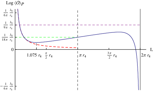
As before, the Polyakov action (i.e., the term in (63)) dominates in the supergravity limit and so we focus on this term in the following. The result depends on all three of the independent parameters, , and (or rather dimensionless ratios of these parameters) — recall that is implicitly defined as a function of the ratio by the relation (47). A natural approach is to hold the gauge theory parameters constant (by fixing the ratio ) and consider the expectation value as a function of , the separation of the defects. This is illustrated in figure 5, where we show as a function of . The plot shows that as approaches zero, our result follows the extremal result, , appearing in the exponential factor in (62). This behaviour arises because for , the branes do not extend very far into the bulk and so the string stretched between them detects no difference between the extremal and non-extremal backgrounds. In terms of the gauge theory, this behaviour simply reflects the fact that the chiral symmetry breaking scale is much larger than the confining scale , where supersymmetry breaking takes effect in the gauge theory. As becomes larger, the calculation begins to probe regions of the dual spacetime geometry closer to and one sees that the extremal and nonextremal behaviours of begin to deviate around . The expectation value reaches an interesting local minimum at , where . Note that the location of the minimum is independent of and is therefore always visible in the supergravity limit.
When reaches , the defects are located at antipodal points on the circle. This corresponds, in the relation (47), to the limiting value . However, we have extended to the region in figure 5. Of course, in this regime, the shortest distance between the defects on the circle is but the open Wilson line stretches the longer distance around the circle.44 4 In principle, the following construction could be extended to consider Wilson lines which connect the defects after fully winding around the circle some number of times. The embedding profile of the D8- pair is identical to those in section 4.1 but with replacing . Now in the expectation value, the dual worldsheet spans the minimal surface ‘outside’ of the U-shape formed by the D8- pair. Hence the (renormalized) Polyakov action may be calculated as the action of a worldsheet covering the entire - geometry (48) minus that for the worldsheet stretched ‘inside’ of the U-shape. As a result, at this order, we have the relation: where is the expectation value of a closed Wilson line which winds once around the circle. (Note that we find .) Figure 5 displays a symmetry about which reflects this relation and we may infer that approaches zero as . Of course, we should add that the five-dimensional gauge theory is defined with a cut-off and so one should not really consider the above results for .
An alternative approach to considering the expectation value , is to consider it as a function of with fixed and . The result is plotted in figure 6 for . In the decompactification limit, , the expectation value again asymptotes to the extremal result . Note that, because is independent of the ratio , this plot can also be understood as showing the dependence of on the four-dimensional ‘t Hooft coupling, using the relation .

5 Discussion
We have examined various aspects of a recent proposal [10, 11, 12] to add quark masses to the Sakai-Sugimoto model with nonlocal operators of the form (21). The underlying microscopic field theory is a five-dimensional gauge theory where the chiral quarks are localized on separate four-dimensional defects. However, the five-dimensional gauge theory is only defined with a cut-off, i.e., new degrees of freedom appear in the far UV. In the dual supergravity background, this issue is realized by the running of the dilaton which produces large string coupling in the asymptotic region. In section 3, we examined modifications introduced by the coupling of the dilaton to the string worldsheet. In particular, we showed that this coupling calls for a modification of the renormalization of these operators as in (42). The first two subtractions, which are linear in the length , renormalize the Wilson line and are not particular to the present open Wilson line calculations. Hence both of these terms, including the second one proportional to , would appear in calculations for closed Wilson lines as well. On the other hand, the log subtraction is distinctive of the two end-points of the open Wilson line.
It is interesting to re-express the subtractions in (42) in terms of an energy cut-off, using the standard dictionary ,
| (64) |
In the third term, is the (dimensionless) effective coupling (9) of the five-dimensional gauge theory evaluated at the cut-off scale . Hence the expansion on the string worldsheet produces an expansion in inverse powers of the coupling from the gauge theory perspective, rather than the expansion as produced by -corrections to the supergravity action — a similar observation was made about the thermal quark diffusion constant in [35]. It is interesting that the energy scale appearing in the second subtraction is the supergravity energy scale associated with [18]. This is a natural energy scale to appear here since fluctuations on the worldsheet are contributing at this order [26].
In section 4, we explicitly calculated the expectation value of the nonlocal fermion bilinear. This expectation value characterizes the chiral condensate in this holographic model. As this holographic construction does not permit the construction of a local fermion bilinear, this expectation value is the best order parameter to characterize the spontaneous breaking of chiral symmetry. Our explicit calculations yield the result given in (63). We note that (7) and (46) can be used to express the pre-factor of the Polyakov term as , up to numerical factors, where is the effective coupling evaluated at the chiral symmetry breaking scale . The dependence of on illustrated in figure 5 describes the intricate interplay of the supersymmetry breaking (or confinement) and chiral symmetry breaking scales in determining the expectation value. Of course, in the absence of supersymmetry breaking, the result in the extremal background (62) is independent of [10]. As figure 5 also illustrates, approaches this supersymmetric result in the limit .
Studying the theory at finite temperature in this regime, one finds that the chiral symmetry breaking and confinement/deconfinement phase transitions are independent [24, 36]. As described in section 2, the chiral symmetry breaking is realized in the gravitational dual by the D8- pair joining together to form a smooth U-shaped embedding. The deconfined phase of the gauge theory is represented by replacing the supergravity background by a D4 black hole [15]. The transition between the low-temperature confining phase and the high-temperature deconfined phase occurs when [15]
| (65) |
In the deconfined phase, if is sufficiently large, the tension of the D8-branes can support the U-shaped embedding against gravitational attraction of the black hole, which has the interpretation that the chiral symmetry remains broken in the deconfined phase [24, 36]. Chiral symmetry is not restored until a temperature given by
| (66) |
where . Above this temperature, the gravitational attraction becomes sufficiently large that the D8- pair are pulled into the horizon (and the embedding is trivial, i.e., ), as shown in figure 7. The phase structure of the Sakai-Sugimoto model is summarized in figure 8.

In the high temperature phase, where the D8- pair is disconnected, the chiral symmetry is restored and so this should be reflected in the expectation value. In particular, beyond the phase transition of [24, 36], one should have . In fact, this result does arise because with the trivial embedding in the black hole background there is no string worldsheet connecting the D8- pair with a single asymptotic boundary. The simplest consistent worldsheet would extend through the ‘Einstein-Rosen’ throat and out to the boundary of the second asymptotic region in the black hole geometry. Hence this worldsheet would be relevant for a correlator of two operators with the second being in the thermofield double of the original gauge theory [37].

In a similar way, these expectation values are useful for characterizing the different phases in theories with many defects, as discussed, e.g., in [38]. Again, one would find for a Wilson line operator connecting two defects which are not dual to a D8- pair which are not joined.
As observed at the end of section 3.1, in accord with the standard large counting. In our calculations, we essentially set the number of flavours to one, however, if one might anticipate the expectation values would also be proportional to , again reflecting the number of degrees of freedom involved in such a bilinear — e.g., , see [34, 39]. However, in the case where , we are implicitly considering the expectation value of an operator with flavour indices and for the two fermions. For the smooth embeddings, we would have because consistency requires that the worldsheet start and end on the same brane throughout the embedding. A priori, there is no connection between the on one defect and the on the other. So our operator reveals this connection as established by the chiral symmetry breaking. Tracing over the flavour indices would correspond to implicitly summing over the different worldsheets and would produce the factor of mentioned above.
An alternate approach to understanding chiral symmetry breaking in the Sakai-Sugimoto model was considered in [6, 7, 8, 9]. There the key element is the open string tachyon that develops between the D8- pair when the (proper) distance separating them is small. Chiral symmetry breaking is realized as the condensation of the tachyon, which leads to brane-anti-brane annihilation deep in the IR region, producing the smooth embedding in which the D8- pair join. The quark mass and the chiral condensate would be related to the asymptotically growing and decaying modes of the tachyon field. This description and the approach examined in the present paper both consider the physics of open strings stretched between the D8- and -branes, so it seems that they must be related. Conceptually, one can think of the tachyon analysis as the second-quantized description of the relevant open string physics while the worldsheet procedure [10, 11, 12] considered above is the first-quantized description of essentially the same physics. Of course, it would be interesting to make this connection more precise. This naturally calls for a proper quantization of (open) strings in the supergravity background of the D4-brane throat. A more accessible route may be to examine the D8-brane embeddings for a nonvanishing quark mass, following the suggestion of [10] to include the Polyakov action for the instantonic worldsheet as part of the action for the D8- pair . One could then consider the dependence of on and compare with the results given in [7, 8, 9].
Acknowledgments.
It is a pleasure to thank Ofer Aharony, Martin Kruczenski, David Kutasov and Arkady Tseytlin for useful correspondence and conversations. RCM would also like to thank Shigeki Sugimoto and especially Rowan Thomson for their collaboration at a very early stage of this project. Research at Perimeter Institute is supported by the Government of Canada through Industry Canada and by the Province of Ontario through the Ministry of Research & Innovation. RCM also acknowledges support from an NSERC Discovery grant and funding from the Canadian Institute for Advanced Research.Appendix A Fluctuation Determinant
In this appendix we will evaluate the contribution from fluctuations for rectangular worldsheet discussed in section 3.1. Since is a loop-counting parameter on the string worldsheet, the one-loop fluctuation determinant will contribute at the same order as the Fradkin-Tseytlin term (27), considered in the main text. The primary result here is to show that the fluctuation determinant contributes no additional UV divergences to the Wilson line calculations, at this order. Since the UV behaviour is universal, this result applies for all of the Wilson line calculations considered in the present paper. A similar analysis of worldsheet fluctuations for a standard closed Wilson line in the D4-brane background has been performed in [40]. To begin the calculation, we must expand the worldsheet action to quadratic order about a classical solution, . Working with the Green-Schwarz formalism,55 5 One might question whether or not the Fradkin-Tseytlin term (27) is to be added in the worldsheet action of the Green-Schwarz string. While the classical action does not couple to the dilaton, this interaction is still necessary at the quantum level to preserve the conformal and symmetry of Green-Schwarz string, just as in the bosonic case (and also to have proper effective string coupling dependence of string loops). this yields
| (67) |
where
| (68) | |||||
| (69) |
and
| (70) |
In the above, labels a spacetime index which we will split in what follows as labeling a direction and labeling the remaining transverse directions. The worldsheet directions will be labeled by lower Greek indices. The other quantities are specified by[40]
| (71) |
| (72) |
where are tangent space indices. The -symmetry transformation for the GS fermions is given by
| (73) |
Note that for simplicity in the following calculations, we will set in the supergravity background. We will also drop the dilaton terms in what follows since they are subleading.
Fermion contributions
We will use the zehnbeins
| (74) | |||||
| (75) | |||||
| (76) | |||||
| (77) |
In the following we will sometimes use the notation . The RR field strength in tangent space is given by
| (78) |
In the case at hand, and where are worldsheet variables. Using the pullback metric for the Euclidean worldsheet and noting that we get
| (79) |
Here we have absorbed into the fluctuations. Using
| (80) | |||||
| (81) | |||||
| (82) |
with in tangent space we get
| (83) | |||||
We will fix -symmetry with the following: First split . Then choose
| (84) |
which leads to after redefining and defining
| (85) |
Now choosing the gamma matrices such that
| (86) |
with being Euclidean Dirac matrices in 8 dimensions and splitting the ’s into two Euclidean Majorana-Weyl fermions of opposite chiralities we get
| (87) |
The squared equations of motion following from the above are:
| (88) | |||||
| (89) |
Combining into a worldsheet spinor , the equations of motion for the fermions then takes on the form
| (90) |
Here represents the Pauli matrix . In first order perturbation theory, the term proportional to will not contribute. Since and combine to form a worldsheet spinor, we have 8 massive fermions satisfying the above equation66 6 Otherwise naively it would appear that there are 8 ’s and 8 ’s giving 16 fermions which would lead to the wrong counting..
Boson contributions
In the second line of (68), we have included the contributions of the Fradkin-Tseytlin term (27). However, these two terms come with explicit factors of the string length which reflects the fact that they would only contribute in a two-loop calculation of the fluctuation determinant. Therefore we ignore these last two contributions in the following calculation. The quadratic order action for the bosons is given by
| (91) | |||||
Here we have defined . Thus the mass terms are at . Hence we now have satisfying
| (92) |
while satisfy
| (93) |
Ghost contributions
The ghost action works out to be
| (94) |
with and . The ghosts satisfy
| (95) | |||||
| (96) |
Final Result
The result for the partition function after the above laborious calculation is
| (97) |
The evaluation of the determinant exactly is in general a very hard problem [41]. In this case we note that (97) can be rewritten as
| (98) |
where and . Then each of the operators featuring in the determinant can be written as [41]
| (99) |
so that we can write the determinant as where is given by
| (100) |
The function satisfies Dirichlet boundary conditions, namely . Here is related to through . The solution to (100) with the Dirichlet boundary conditions are known to be Bessel functions , . Since both are allowed, we will choose and to be the independent solutions. Then imposing the boundary condition at we have
| (101) | |||||
| (102) |
so that ’s are related to the zeros of the Bessel functions. Then the determinant can be written using the formula
| (103) |
as
| (104) |
where
| (105) | |||||
| (106) |
Now we want to get the large asymptotics of this function. We use the useful identity[42] that the large zeros of the Bessel function behave as
| (107) |
to get
| (108) | |||||
using which the leading divergence cancels. The subleading terms arise from terms which lead to a finite result at . The exact formula (104) allows us in principle to extract this finite number although we will not attempt it here, as this contribution would vanish in the relevant limit . Hence our key result is that in the fluctuation determinant (97) is in fact precisely 1 in this limit.
References
- [1] J.M. Maldacena, “The large N limit of superconformal field theories and supergravity,” Adv. Theor. Math. Phys. 2, 231 (1998) [Int. J. Theor. Phys. 38, 1113 (1999)] [arXiv:hep-th/9711200].
- [2] O. Aharony, S.S. Gubser, J.M. Maldacena, H. Ooguri and Y. Oz, “Large N field theories, string theory and gravity,” Phys. Rept. 323, 183 (2000) [arXiv:hep-th/9905111].
- [3] T. Sakai and S. Sugimoto, “Low energy hadron physics in holographic QCD,” Prog. Theor. Phys. 113, 843 (2005) [arXiv:hep-th/0412141].
- [4] T. Sakai and S. Sugimoto, “More on a holographic dual of QCD,” Prog. Theor. Phys. 114, 1083 (2006) [arXiv:hep-th/0507073].
- [5] K. Hashimoto, T. Hirayama and A. Miwa, “Holographic QCD and pion mass,” JHEP 0706, 020 (2007) [arXiv:hep-th/0703024].
- [6] R. Casero, E. Kiritsis and A. Paredes, “Chiral symmetry breaking as open string tachyon condensation,” Nucl. Phys. B 787, 98 (2007) [arXiv:hep-th/0702155].
- [7] O. Bergman, S. Seki and J. Sonnenschein, “Quark mass and condensate in HQCD,” JHEP 0712, 037 (2007) [arXiv:0708.2839 [hep-th]].
- [8] A. Dhar and P. Nag, “Sakai-Sugimoto model, Tachyon Condensation and Chiral symmetry Breaking,” JHEP 0801, 055 (2008) [arXiv:0708.3233 [hep-th]].
- [9] A. Dhar and P. Nag, “Tachyon condensation and quark mass in modified Sakai-Sugimoto model,” arXiv:0804.4807 [hep-th].
- [10] O. Aharony and D. Kutasov, “Holographic Duals of Long Open Strings,” arXiv:0803.3547 [hep-th].
- [11] K. Hashimoto, T. Hirayama, F. L. Lin and H. U. Yee, “Quark Mass Deformation of Holographic Massless QCD,” arXiv:0803.4192 [hep-th].
- [12] R. C. Myers and R. M. Thomson, unpublished.
- [13] J. M. Maldacena, “Wilson loops in large N field theories,” Phys. Rev. Lett. 80, 4859 (1998) [arXiv:hep-th/9803002].
- [14] S. J. Rey and J. T. Yee, “Macroscopic strings as heavy quarks in large N gauge theory and anti-de Sitter supergravity,” Eur. Phys. J. C 22, 379 (2001) [arXiv:hep-th/9803001].
- [15] E. Witten, “Anti-de Sitter space, thermal phase transition, and confinement in gauge theories,” Adv. Theor. Math. Phys. 2, 505 (1998) [arXiv:hep-th/9803131].
- [16] G. T. Horowitz and R. C. Myers, “The AdS/CFT correspondence and a new positive energy conjecture for general relativity,” Phys. Rev. D 59, 026005 (1999) [arXiv:hep-th/9808079].
- [17] N. Itzhaki, J.M. Maldacena, J. Sonnenschein and S. Yankielowicz, “Supergravity and the large N limit of theories with sixteen supercharges,” Phys. Rev. D 58, 046004 (1998) [arXiv:hep-th/9802042].
- [18] A.W. Peet and J. Polchinski, “UV/IR relations in AdS dynamics,” Phys. Rev. D 59, 065011 (1999) [arXiv:hep-th/9809022].
- [19] C. Csaki, H. Ooguri, Y. Oz and J. Terning, “Glueball mass spectrum from supergravity,” JHEP 9901, 017 (1999) [arXiv:hep-th/9806021].
- [20] M. Kruczenski, D. Mateos, R.C. Myers and D.J. Winters, “Towards a holographic dual of large-N(c) QCD,” JHEP 0405, 041 (2004) [arXiv:hep-th/0311270].
- [21] B. A. Burrington, V. S. Kaplunovsky and J. Sonnenschein, “Localized Backreacted Flavor Branes in Holographic QCD,” JHEP 0802, 001 (2008) [arXiv:0708.1234 [hep-th]].
- [22] E. Antonyan, J. A. Harvey, S. Jensen and D. Kutasov, “NJL and QCD from string theory,” arXiv:hep-th/0604017.
- [23] K. Peeters, J. Sonnenschein and M. Zamaklar, “Holographic decays of large-spin mesons,” JHEP 0602, 009 (2006) [arXiv:hep-th/0511044].
- [24] O. Aharony, J. Sonnenschein and S. Yankielowicz, “A holographic model of deconfinement and chiral symmetry restoration,” Annals Phys. 322, 1420 (2007) [arXiv:hep-th/0604161].
- [25] R. M. Thomson, unpublished.
- [26] R. C. Myers and R. M. Thomson, “Holographic mesons in various dimensions,” JHEP 0609, 066 (2006) [arXiv:hep-th/0605017].
- [27] N. Drukker, D.J. Gross and H. Ooguri, “Wilson loops and minimal surfaces,” Phys. Rev. D 60, 125006 (1999) [arXiv:hep-th/9904191].
- [28] N. Drukker and B. Fiol, “All-genus calculation of Wilson loops using D-branes,” JHEP 0502, 010 (2005) [arXiv:hep-th/0501109].
- [29] A. Brandhuber, N. Itzhaki, J. Sonnenschein and S. Yankielowicz, “Wilson loops, confinement, and phase transitions in large N gauge theories from supergravity,” JHEP 9806 (1998) 001 [arXiv:hep-th/9803263].
- [30] O. Bergman and G. Lifschytz, “Holographic U(1)A and string creation,” JHEP 0704, 043 (2007) [arXiv:hep-th/0612289].
- [31] E. S. Fradkin and A. A. Tseytlin, “Quantum String Theory Effective Action,” Nucl. Phys. B 261, 1 (1985).
- [32] J. Polchinski,“String theory. Vol. 1: An introduction to the bosonic string,” Cambridge University Press (2001).
- [33] A. Karch, A. O’Bannon and K. Skenderis, “Holographic renormalization of probe D-branes in AdS/CFT,” JHEP 0604, 015 (2006) [arXiv:hep-th/0512125].
- [34] D. Mateos, R. C. Myers and R. M. Thomson, “Thermodynamics of the brane,” JHEP 0705, 067 (2007) [arXiv:hep-th/0701132].
- [35] R. C. Myers, A. O. Starinets and R. M. Thomson, “Holographic spectral functions and diffusion constants for fundamental matter,” JHEP 0711, 091 (2007) [arXiv:0706.0162 [hep-th]].
- [36] A. Parnachev and D. A. Sahakyan, “Chiral phase transition from string theory,” Phys. Rev. Lett. 97, 111601 (2006) [arXiv:hep-th/0604173].
- [37] J. M. Maldacena, “Eternal black holes in Anti-de-Sitter,” JHEP 0304, 021 (2003) [arXiv:hep-th/0106112].
- [38] A. Basu and A. Maharana, “Generalized Gross-Neveu models and chiral symmetry breaking from string theory,” Phys. Rev. D 75, 065005 (2007) [arXiv:hep-th/0610087].
- [39] S. Kobayashi, D. Mateos, S. Matsuura, R. C. Myers and R. M. Thomson, “Holographic phase transitions at finite baryon density,” JHEP 0702, 016 (2007) [arXiv:hep-th/0611099].
- [40] F. Bigazzi, A. L. Cotrone, L. Martucci and L. A. Pando Zayas, “Wilson loop, Regge trajectory and hadron masses in a Yang-Mills theory from semiclassical strings,” Phys. Rev. D 71, 066002 (2005) [arXiv:hep-th/0409205].
- [41] G. V. Dunne, “Functional Determinants in Quantum Field Theory,” arXiv:0711.1178 [hep-th].
- [42] G. N. Watson, “Theory of Bessel Functions,” Cambridge University Press, 1922.