跳到论文正文
W Papers独立论文阅读器 arXiv:0807.5117 论文正文 计算阅读时间 · 0%
引用这篇论文根据当前论文元数据生成,正式投稿前建议核对。


License: arXiv.org perpetual non-exclusive license
arXiv:0807.5117v1 [math.KT] 31 Jul 2008

Formality of the homotopy calculus algebra of Hochschild (co)chains

Vasiliy Dolgushev    Dmitry Tamarkin    Boris Tsygan
Abstract

The Kontsevich-Soibelman solution of the cyclic version of Deligne’s conjecture and the formality of the operad of little discs on a cylinder provide us with a natural homotopy calculus structure on the pair (C∙​(A),C∙​(A))(C^{\bullet}(A),C_{\bullet}(A)) “Hochschild cochains ++ Hochschild chains” of an associative algebra AA. We show that for an arbitrary smooth algebraic variety XX over a field 𝕂{\mathbb{K}} of characteristic zero the sheaf (C∙​(𝒪X),C∙​(𝒪X))(C^{\bullet}({\cal O}_{X}),C_{\bullet}({\cal O}_{X})) of homotopy calculi is formal. This result was announced in paper [29] by the second and the third author.

To Mikhail Olshanetsky on the occasion of his 70th birthday.

1 Introduction

The standard Cartan calculus on polyvector fields and exterior forms can be naturally extended to the Hochschild cohomology H​H∙​(A,A)HH^{{\bullet}}(A,A) and the Hochschild homology H​H∙​(A,A)HH_{{\bullet}}(A,A) of an arbitrary associative algebra AA [11], [24]. This calculus is induced by simple operations on Hochschild (co)chains, and the identities of this algebraic structure hold for these operations up to homotopy.

The Kontsevich-Soibelman proof of the cyclic version of Deligne’s conjecture [23] and the formality of the operad of little discs on a cylinder11 1 See Proposition 11.3.3 on page 50 in [23]. imply that this nice collection of the operations on the pair (Cnorm∙​(A),C∙norm​(A))(C^{\bullet}_{{\rm norm}}(A),C_{\bullet}^{{\rm norm}}(A)) “(normalized) Hochschild cochains ++ (normalized) Hochschild chains” can be extended to an ∞\infty- or homotopy calculus structure.

This homotopy calculus structure on the pair (Cnorm∙​(A),C∙norm​(A))(C^{\bullet}_{{\rm norm}}(A),C_{\bullet}^{{\rm norm}}(A)) is a natural generalization of the homotopy Gerstenhaber algebra structure on the cochains Cnorm∙​(A)C^{\bullet}_{{\rm norm}}(A) . In paper [13] we proved the formality of this homotopy Gerstenhaber algebra on Cnorm∙​(A)C^{\bullet}_{{\rm norm}}(A) for an arbitrary regular commutative algebra AA over a field 𝕂{\mathbb{K}} of characteristic zero. In this paper we extend this result to the homotopy calculus algebra on the pair (Cnorm∙​(A),C∙norm​(A))(C^{\bullet}_{{\rm norm}}(A),C_{\bullet}^{{\rm norm}}(A)) .

As well as in [13] we also consider the situation when the algebra AA is replaced by the structure sheaf 𝒪X{\cal O}_{X} of a smooth algebraic variety XX over the field 𝕂{\mathbb{K}} . More precisely, we consider the homotopy calculus algebra on the pair (Cnorm∙​(𝒪X),C∙norm​(𝒪X))(C^{\bullet}_{{\rm norm}}({\cal O}_{X}),C_{\bullet}^{{\rm norm}}({\cal O}_{X})) where Cnorm∙​(𝒪X)C^{\bullet}_{{\rm norm}}({\cal O}_{X}) and C∙norm​(𝒪X)C_{\bullet}^{{\rm norm}}({\cal O}_{X}) is, respectively, the sheaf of (normalized) Hochschild cochains and the sheaf of (normalized) Hochschild chains of 𝒪X{\cal O}_{X} . In this paper we show that the sheaf of homotopy calculi (Cnorm∙​(𝒪X),C∙norm​(𝒪X))(C^{\bullet}_{{\rm norm}}({\cal O}_{X}),C_{\bullet}^{{\rm norm}}({\cal O}_{X})) is formal.

If AA is an associative algebra (with unit), the pair (Cnorm∙​(A),C∙norm​(A))(C^{\bullet}_{{\rm norm}}(A),C_{\bullet}^{{\rm norm}}(A)) is also equipped with an algebraic structure defined by a degree −1-1 Lie bracket on Cnorm∙​(A)C^{\bullet}_{{\rm norm}}(A) , a degree −1-1 Lie module structure on C∙norm​(A)C_{\bullet}^{{\rm norm}}(A) over Cnorm∙​(A)C^{\bullet}_{{\rm norm}}(A) , and Connes’ operator on C∙norm​(A)C_{\bullet}^{{\rm norm}}(A) which is compatible with the Lie module structure. In the paper we refer to such algebra structures as Λ​𝐋𝐢𝐞δ+{\Lambda}{\bf Lie}^{+}_{{\delta}}-algebra. (See Definition 4.)

In paper [31] the third author conjectured that if AA is a regular commutative algebra then this Λ​𝐋𝐢𝐞δ+{\Lambda}{\bf Lie}^{+}_{{\delta}}-algebra structure on (Cnorm∙​(A),C∙norm​(A))(C^{\bullet}_{{\rm norm}}(A),C_{\bullet}^{{\rm norm}}(A)) is formal. This conjecture was proved in [33] (at least in the case ℝ⊂𝕂{\mathbb{R}}\subset{\mathbb{K}}) by Willwacher who used the constructions of B. Shoikhet [25] and the first author [12].

In general H​o​(Λ​𝐋𝐢𝐞δ+)Ho({\Lambda}{\bf Lie}^{+}_{{\delta}})-part of the homotopy calculus structure on (Cnorm∙​(A),C∙norm​(A))(C^{\bullet}_{{\rm norm}}(A),C_{\bullet}^{{\rm norm}}(A)) derived from [23] may not coincide with the Λ​𝐋𝐢𝐞δ+{\Lambda}{\bf Lie}^{+}_{{\delta}}-algebra on the pair (Cnorm∙​(A),C∙norm​(A))(C^{\bullet}_{{\rm norm}}(A),C_{\bullet}^{{\rm norm}}(A)) . However, we show that this homotopy calculus algebra on (Cnorm∙​(A),C∙norm​(A))(C^{\bullet}_{{\rm norm}}(A),C_{\bullet}^{{\rm norm}}(A)) is quasi-isomorphic to another homotopy calculus algebra on (Cnorm∙​(A),C∙norm​(A))(C^{\bullet}_{{\rm norm}}(A),C_{\bullet}^{{\rm norm}}(A)) whose H​o​(Λ​𝐋𝐢𝐞δ+)Ho({\Lambda}{\bf Lie}^{+}_{{\delta}})-part is the ordinary Λ​𝐋𝐢𝐞δ+{\Lambda}{\bf Lie}^{+}_{{\delta}}-algebra given by the above Lie bracket on Cnorm∙​(A)C^{\bullet}_{{\rm norm}}(A), the Lie algebra module on C∙norm​(A)C_{\bullet}^{{\rm norm}}(A) over Cnorm∙​(A)C^{\bullet}_{{\rm norm}}(A) and Connes’ operator on C∙norm​(A)C_{\bullet}^{{\rm norm}}(A) . In this sense, the formality of the homotopy calculus algebra on (Cnorm∙​(A),C∙norm​(A))(C^{\bullet}_{{\rm norm}}(A),C_{\bullet}^{{\rm norm}}(A)) is a generalization of Willwacher’s cyclic formality theorem [33].

The organization of the paper is as follows. In Section 2 we fix the notation and recall required results about (co)operads and (co)algebras. Section 3 is devoted to ∞\infty- or homotopy versions for the algebras over the operads 𝐜𝐚𝐥𝐜{\bf calc} , 𝐞𝟐{\bf e_{2}} , and 𝐋𝐢𝐞δ+{\bf Lie}^{+}_{{\delta}} . In Section 4 we recall the Kontsevich-Soibelman operad and the operad Cyl{\rm Cyl}\, of little discs on a cylinder. We show that the homology operad H−⁣∙​(Cyl,𝕂)H_{-{\bullet}}({\rm Cyl}\,,{\mathbb{K}}) of Cyl{\rm Cyl}\, with the reversed grading is the operad of calculi. Finally we recall required results from [23] and prove a useful property of the Kontsevich-Soibelman operad. Section 5 is devoted to properties of the homotopy calculus algebra on the pair (Cnorm∙​(A),C∙norm​(A))(C^{\bullet}_{{\rm norm}}(A),C_{\bullet}^{{\rm norm}}(A)) . In Section 6 we formulate and prove the main result of this paper. (See Theorem 5 on page 5.) In the concluding section we discussion applications and generalizations of Theorem 5. We also discuss recent articles related to our main result.

Acknowledgment. A bigger part of this work was done when V.D. was a Boas Assistant Professor of Mathematics Department at Northwestern University. During these two years V.D. benefited from working at Northwestern so much that he feels as if he finished one more graduate school. V.D. cordially thanks Mathematics Department at Northwestern University for this time. The results of this work were presented at the conference Poisson 2008 in Lausanne. We would like to thank the participants of this conference for questions and useful comments. V.D. would like to thank Pavel Snopok for showing him a very convenient drawing program “Inkscape”. D.T. and B.T. are supported by NSF grants. The work of V.D. is partially supported by the Grant for Support of Scientific Schools NSh-8065.2006.2.

2 Preliminaries

2.1 (Co)operads and (co)algebras

Most of the notation and conventions for (co)operads and their (co)algebras are borrowed from [13].

Depending on a context our underlying symmetric monoidal category is either the category of graded vector spaces, or the category of chain complexes, or the category of compactly generated topological spaces, or the category of sets. By suspension 𝐬​𝒱{\bf s}\,{\cal V} of a graded vector space (or a chain complex) 𝒱{\cal V} we mean ε⊗𝒱{\varepsilon}\otimes{\cal V}, where ε{\varepsilon} is a one-dimensional vector space placed in degree +1+1 . For a vector v∈𝒱v\in{\cal V} we denote by |v||v| its degree. The symmetric group of permutations of nn letters is denoted by SnS_{n} . The underlying field 𝕂{\mathbb{K}} has characteristic zero.

For an operad 𝒪{\cal O} we denote by Alg𝒪{\rm Alg}\,_{{\cal O}} the category of algebras over the operad 𝒪{\cal O}. Dually, for a cooperad 𝒞{\cal C} we denote by Coalg𝒞{\rm Coalg}\,_{{\cal C}} the category of nilpotent22 2 For the definition of nilpotent coalgebra see section 2.4.12.4.1 in [19]. coalgebras over the cooperad 𝒞{\cal C} . By corestriction we mean the canonical map

ρ𝒱:𝔽𝒞​(𝒱)→𝒱\rho_{{\cal V}}:{\mathbb{F}}_{{\cal C}}({\cal V})\to{\cal V} (2.1)

from the free coalgebra 𝔽𝒞​(𝒱){\mathbb{F}}_{{\cal C}}({\cal V}) to the vector space of its cogenerators 𝒱{\cal V} . We often omit the subscript in the notation ρ𝒱\rho_{{\cal V}} for the corestriction.

For a polynomial functor 𝒫{\cal P} we denote by 𝕋⁡(𝒫){\mathbb{T}}({\cal P}) (resp. 𝕋∗​(𝒫){\mathbb{T}}^{*}({\cal P})) the free operad (resp. the free cooperad) (co)generated by 𝒫{\cal P} . The notation ∙\bullet is reserved for the monoidal product of the polynomial functors. Thus, if 𝒫{\cal P} and 𝒬{\cal Q} are polynomial functors then

𝒫∙𝒬⁡(n)=⨁k1+⋯+km=n𝒫⁡(m)⊗Sm(𝒬⁡(k1)⊗⋯⊗𝒬⁡(km)).{\cal P}\bullet{\cal Q}(n)=\bigoplus_{k_{1}+\dots+k_{m}=n}{\cal P}(m)\otimes_{S_{m}}({\cal Q}(k_{1})\otimes\dots\otimes{\cal Q}(k_{m}))\,. (2.2)

This formula can be easily generalized to the colored polynomial functors.

By “suspension” of a (co)operad 𝒪{\cal O} of graded vector spaces (or chain complexes) we mean the (co)operad Λ⁡(𝒪){\Lambda}({\cal O}) whose mm-th vector space is

Λ⁡(𝒪)​(m)=𝐬1−m​𝒪​(m)⊗sgnm,{\Lambda}({\cal O})(m)={\bf s}\,^{1-m}{\cal O}(m)\otimes{\rm sgn}_{m}\,, (2.3)

where sgnm{\rm sgn}_{m} is the sign representation of the symmetric group SmS_{m} .

For a commutative algebra ℬ{\cal B} and a ℬ{\cal B}-module 𝒱{\cal V} we denote by Sℬ​(𝒱)S_{{\cal B}}({\cal V}) the symmetric algebra of 𝒱{\cal V} over ℬ{\cal B} . Sℬm​(𝒱)S_{{\cal B}}^{m}({\cal V}) stands for the mm-th component of this algebra. If ℬ=𝕂{\cal B}={\mathbb{K}} then ℬ{\cal B} is omitted from the notation. The abbreviation “DGLA” stands for differential graded Lie algebra.

We denote by ∗\ast the polynomial functor

∗(n)={𝕂,if​n=1,0,otherwise.\ast(n)=\begin{cases}{\mathbb{K}}\,,\qquad{\rm if}~~n=1\,,\\ 0\,,\qquad{\rm otherwise}\,.\end{cases} (2.4)

This functor carries the unique structure of the operad (resp. the cooperad) such that ∗\ast is the initial (resp. the terminal) object in the category of operads (resp. cooperads) of graded vector spaces or chain complexes. There is an obvious generalization of ∗\ast (2.4) to the category of sets and to the category of topological spaces. However, we will need ∗\ast only for linear (co)operads, i.e. the (co)operads in the category of graded vector spaces or the category of chain complexes.

All the linear operads (resp. linear cooperads), we consider, are equipped with an augmentation (resp. coaugmentation). In other words, for every operad 𝒪{\cal O} we will have a chosen morphism of operads:

τ:𝒪→∗.\tau\,:\,{\cal O}\to\ast\,. (2.5)

Dually for every cooperad 𝒞{\cal C} we will have a chosen morphism of cooperads

κ:∗→𝒞.{\kappa}\,:\,\ast\to{\cal C}\,. (2.6)

We are going to deal with 22-colored (co)operads. Throughout the paper we label the two colors of all 22-colored (co)operads by 𝔠{\mathfrak{c}} and 𝔞{\mathfrak{a}} . For example, the notation 𝐋𝐢𝐞+{\bf Lie}^{+} is reserved for the 22-colored operad which governs the pairs “Lie algebra 𝒱{\cal V} and a Lie algebra module 𝒲{\cal W} over 𝒱{\cal V} .” Vectors of the Lie algebra 𝒱{\cal V} are colored by 𝔠{\mathfrak{c}} and vectors of the module 𝒲{\cal W} are colored by 𝔞{\mathfrak{a}} .

For a linear 22-colored operad 𝒪{\cal O} we will denote by 𝒪𝔠​(n,k){\cal O}^{{\mathfrak{c}}}(n,k) (resp. 𝒪𝔞​(n,k){\cal O}^{{\mathfrak{a}}}(n,k)) the vector space of operations producing a vector with the color 𝔠{\mathfrak{c}} (resp. 𝔞{\mathfrak{a}}) from nn vectors with the color 𝔠{\mathfrak{c}} and kk vectors with the color 𝔞{\mathfrak{a}} . We use the same notation for the linear 22-colored cooperads and for topological 22-colored operads.

The polynomial functor ∗\ast (2.4) has the obvious generalization to the category of linear 22-colored (co)operads:

∗𝔠(n,k)={𝕂,if⁡(n,k)=(1,0),0,otherwise.∗𝔞(n,k)={𝕂,if⁡(n,k)=(0,1),0,otherwise.\begin{array}[]{c}\ast^{{\mathfrak{c}}}(n,k)=\begin{cases}{\mathbb{K}}\,,\qquad{\rm if}~~(n,k)=(1,0)\,,\\ 0\,,\qquad{\rm otherwise}\,.\end{cases}\\[14.22636pt] \ast^{{\mathfrak{a}}}(n,k)=\begin{cases}{\mathbb{K}}\,,\qquad{\rm if}~~(n,k)=(0,1)\,,\\ 0\,,\qquad{\rm otherwise}\,.\end{cases}\end{array} (2.7)

For a linear operad 𝒪{\cal O} we denote by B​a​r​(𝒪)Bar({\cal O}) its bar construction. Dually, for a linear cooperad 𝒞{\cal C} we denote by C​o​b​a​r​(𝒞)Cobar({\cal C}) its cobar construction.

We recall that, as a cooperad of graded vector spaces, B​a​r​(𝒪)Bar({\cal O}) is freely generated by the polynomial functor 𝐬−1​𝒪¯{\bf s}\,^{-1}\overline{\cal O} , where 𝒪¯\overline{\cal O} is the kernel of the augmentation (2.5). Dually, as an operad of graded vector spaces, C​o​b​a​r​(𝒞)Cobar({\cal C}) is freely generated by the polynomial functor 𝐬​𝒞¯{\bf s}\,\overline{\cal C} , where 𝒞¯\overline{\cal C} is cokernel of the coaugmentation (2.6). The differential ∂B​a​r{\partial}^{Bar} on the operad B​a​r​(𝒪)Bar({\cal O}) is defined using the multiplication of the operad 𝒪{\cal O} and the differential ∂C​o​b​a​r{\partial}^{Cobar} on the cooperad C​o​b​a​r​(𝒞)Cobar({\cal C}) is defined using the comultiplication of the cooperad 𝒞{\cal C} . See Chapter 3 in [15] or Section 2 in [17] for details.

For a quadratic operad 𝒪{\cal O} there is a natural sub-cooperad 𝒪∨{\cal O}^{\vee} of B​a​r​(𝒪)Bar({\cal O}) which satisfies the property:

∂B​a​r|𝒪∨=0.{\partial}^{Bar}\Big|_{{\cal O}^{\vee}}=0\,.

The details of the construction of 𝒪∨{\cal O}^{\vee} can be found in Section 5.2 in [15]. Following [18] we call 𝒪∨{\cal O}^{\vee} the Koszul dual cooperad of 𝒪{\cal O} .

For a linear operad 𝒪{\cal O} (resp. linear cooperad 𝒞{\cal C}) and a vector space 𝒱{\cal V} we denote by 𝔽𝒪​(𝒱){\mathbb{F}}_{{\cal O}}({\cal V}) (resp. by 𝔽𝒞​(𝒱){\mathbb{F}}_{{\cal C}}({\cal V})) the free algebra (resp. free coalgebra) over the operad 𝒪{\cal O} (resp. cooperad 𝒞{\cal C}). For a linear 22-colored (co)operad 𝒪{\cal O} the functor33 3 𝔽𝒪{\mathbb{F}}_{{\cal O}} is called the Schur functor. 𝔽𝒪{\mathbb{F}}_{{\cal O}} splits according to the colors 𝔠{\mathfrak{c}} and 𝔞{\mathfrak{a}} as

𝔽𝒪​(𝒱,𝒲)=𝔽𝒪​(𝒱,𝒲)𝔠⊕𝔽𝒪​(𝒱,𝒲)𝔞,{\mathbb{F}}_{{\cal O}}({\cal V},{\cal W})={\mathbb{F}}_{{\cal O}}({\cal V},{\cal W})_{{\mathfrak{c}}}\oplus{\mathbb{F}}_{{\cal O}}({\cal V},{\cal W})_{{\mathfrak{a}}}\,,

where

𝔽𝒪​(𝒱,𝒲)𝔠=⨁n,k𝒪𝔠​(n,k)⊗Sn×Sk𝒱⊗n⊗𝒲⊗k,{\mathbb{F}}_{{\cal O}}({\cal V},{\cal W})_{{\mathfrak{c}}}=\bigoplus_{n,k}{\cal O}^{{\mathfrak{c}}}(n,k)\otimes_{S_{n}\times S_{k}}{\cal V}^{\otimes\,n}\otimes{\cal W}^{\otimes\,k}\,,

and

𝔽𝒪​(𝒱,𝒲)𝔞=⨁n,k𝒪𝔞​(n,k)⊗Sn×Sk𝒱⊗n⊗𝒲⊗k.{\mathbb{F}}_{{\cal O}}({\cal V},{\cal W})_{{\mathfrak{a}}}=\bigoplus_{n,k}{\cal O}^{{\mathfrak{a}}}(n,k)\otimes_{S_{n}\times S_{k}}{\cal V}^{\otimes\,n}\otimes{\cal W}^{\otimes\,k}\,.

We need to recall some facts about algebras over the operad C​o​b​a​r​(𝒞)Cobar({\cal C}) for a coaugmented cooperad 𝒞{\cal C} .

Since C​o​b​a​r​(𝒞)Cobar({\cal C}) is freely generated by the suspension 𝐬​𝒞¯{\bf s}\,\overline{\cal C} of the cokernel 𝒞¯\overline{\cal C} of the coaugmentation (2.6) a C​o​b​a​r​(𝒞)Cobar({\cal C})-algebra structure on a chain complex 𝒱{\cal V} is uniquely determined by the restriction of the multiplication map

μ:𝔽C​o​b​a​r​(𝒞)​(𝒱)→𝒱\mu:{\mathbb{F}}_{Cobar({\cal C})}({\cal V})\to{\cal V}

to the subspace

𝔽𝐬​𝒞¯​(𝒱)⊂𝔽C​o​b​a​r​(𝒞)​(𝒱).{\mathbb{F}}_{{\bf s}\,\overline{\cal C}}({\cal V})\subset{\mathbb{F}}_{Cobar({\cal C})}({\cal V})\,.

In other words, a C​o​b​a​r​(𝒞)Cobar({\cal C})-algebra structure on 𝒱{\cal V} is uniquely determined by a degree 11 map from 𝔽​(𝒞¯)​(𝒱){\mathbb{F}}(\overline{\cal C})({\cal V}) to 𝒱{\cal V} .

It turns out that the maps from 𝔽​(𝒞¯)​(𝒱){\mathbb{F}}(\overline{\cal C})({\cal V}) to 𝒱{\cal V} have a elegant description in terms of coderivations of the free coalgebra 𝔽𝒞​(𝒱){\mathbb{F}}_{{\cal C}}({\cal V}) . To recall this description we introduce the Lie subalgebra

Coder′​(𝔽𝒞​(𝒱))={Q∈Coder⁡(𝔽𝒞​(𝒱))|Q|𝒱=0},\rm Coder^{\prime}({\mathbb{F}}_{{\cal C}}({\cal V}))=\{Q\in\rm Coder({\mathbb{F}}_{{\cal C}}({\cal V}))~|~Q\Big|_{{\cal V}}=0\}\,, (2.8)

where 𝒱{\cal V} is considered as a subspace of 𝒞⁡(1)⊗𝒱{\cal C}(1)\otimes{\cal V} via the coaugmentation (2.6) . In other words, the elements of Coder′​(𝔽𝒞​(𝒱))\rm Coder^{\prime}({\mathbb{F}}_{{\cal C}}({\cal V})) are coderivations of the free coalgebra 𝔽𝒞​(𝒱){\mathbb{F}}_{{\cal C}}({\cal V}) which can be factored through the projection

𝔽𝒞​(𝒱)→𝔽𝒞¯​(𝒱).{\mathbb{F}}_{{\cal C}}({\cal V})\to{\mathbb{F}}_{\overline{\cal C}}({\cal V})\,.

It is not hard to see that the subspace (2.8) is closed under the commutator and the differentials coming from 𝒞{\cal C} and 𝒱{\cal V} . Thus the graded vector space Coder′​(𝔽𝒞​(𝒱))\rm Coder^{\prime}({\mathbb{F}}_{{\cal C}}({\cal V})) is in fact a DGLA.

Let us recall from [17] the following proposition

Proposition 1 (Proposition 2.14 [17])

For a coaugmented cooperad 𝒞{\cal C} the composition with the corestriction (2.1) ρ𝒱:𝔽𝒞​(𝒱)→𝒱\rho_{{\cal V}}:{\mathbb{F}}_{{\cal C}}({\cal V})\to{\cal V} induces an isomorphism of graded vector spaces

C​o​d​e​r′​(𝔽𝒞​(𝒱))≅Hom⁡(𝔽𝒞¯​(𝒱),𝒱),Coder^{\prime}({\mathbb{F}}_{{\cal C}}({\cal V}))\cong{\rm Hom}\,({\mathbb{F}}_{\overline{\cal C}}({\cal V}),{\cal V})\,, (2.9)

where, as above, 𝒞¯\overline{\cal C} is the cokernel of the coaugmentation (2.6) of 𝒞{\cal C} .

Due to this proposition a C​o​b​a​r​(𝒞)Cobar({\cal C})-algebra structure on a chain complex 𝒱{\cal V} is uniquely determined by a degree 11 coderivation

Q∈C​o​d​e​r′​(𝔽𝒞​(𝒱)).Q\in Coder^{\prime}({\mathbb{F}}_{{\cal C}}({\cal V}))\,. (2.10)

According to Proposition 2.15 from [17] the compatibility of the C​o​b​a​r​(𝒞)Cobar({\cal C})-algebra structure on 𝒱{\cal V} with the total differential on C​o​b​a​r​(𝒞)Cobar({\cal C}) and the differential on 𝒱{\cal V} is equivalent to the Maurer-Cartan equation for the corresponding derivation (2.10):

[∂𝒞+∂𝒱,Q]+12[Q,Q]=0,[{\partial}^{{\cal C}}+{\partial}^{{\cal V}},Q]+\frac{1}{2}[Q,Q]=0\,, (2.11)

where ∂𝒞{\partial}^{{\cal C}} is the differential on 𝔽𝒞​(𝒱){\mathbb{F}}_{{\cal C}}({\cal V}) induced by the one on the cooperad 𝒞{\cal C} and ∂𝒱{\partial}^{{\cal V}} comes from that on 𝒱{\cal V} .

In other words,

Proposition 2 (Proposition 2.15, [17])

There is a natural bijection between the Maurer-Cartan elements of the DGLA C​o​d​e​r′​(𝔽𝒞​(𝒱))Coder^{\prime}({\mathbb{F}}_{{\cal C}}({\cal V})) and and the C​o​b​a​r​(𝒞)Cobar({\cal C})-algebra structures on 𝒱{\cal V}.

If we have a map

μ:𝒞1→𝒞2\mu:{\cal C}_{1}\to{\cal C}_{2} (2.12)

of coaugmented cooperads then the corresponding map between the cobar constructions

C​o​b​a​r​(μ):C​o​b​a​r​(𝒞1)→C​o​b​a​r​(𝒞2)Cobar(\mu):Cobar({\cal C}_{1})\to Cobar({\cal C}_{2})

allows us to pull C​o​b​a​r​(𝒞2)Cobar({\cal C}_{2})-algebra structure on 𝒱{\cal V} to a C​o​b​a​r​(𝒞1)Cobar({\cal C}_{1})-algebra on 𝒱{\cal V} .

We claim that

Proposition 3

If Q1Q_{1} is a Maurer-Cartan element of the DGLA C​o​d​e​r′​(𝔽𝒞1​(𝒱))Coder^{\prime}({\mathbb{F}}_{{\cal C}_{1}}({\cal V})) corresponding to a C​o​b​a​r​(𝒞1)Cobar({\cal C}_{1})-algebra structure on 𝒱{\cal V} and Q2Q_{2} is a Maurer-Cartan element of the DGLA C​o​d​e​r′​(𝔽𝒞2​(𝒱))Coder^{\prime}({\mathbb{F}}_{{\cal C}_{2}}({\cal V})) corresponding to a C​o​b​a​r​(𝒞2)Cobar({\cal C}_{2})-algebra structure on 𝒱{\cal V} then

ρ𝒱∘Q1=ρ𝒱∘Q2∘𝔽⁡(μ),\rho_{{\cal V}}\circ Q_{1}=\rho_{{\cal V}}\circ Q_{2}\circ{\mathbb{F}}(\mu)\,, (2.13)

where the map

𝔽⁡(μ):𝔽𝒞¯∞​(𝒱)→𝔽𝒞¯∈​(𝒱){\mathbb{F}}(\mu):{\mathbb{F}}_{\overline{\cal C}_{1}}({\cal V})\to{\mathbb{F}}_{\overline{\cal C}_{2}}({\cal V})

is induced by (2.12) .

Proof. Let

ν2:𝔽C​o​b​a​r​(𝒞2)​(𝒱)→𝒱\nu_{2}:{\mathbb{F}}_{Cobar({\cal C}_{2})}({\cal V})\to{\cal V}

be the C​o​b​a​r​(𝒞2)Cobar({\cal C}_{2})-algebra structure on 𝒱{\cal V} . Then the C​o​b​a​r​(𝒞1)Cobar({\cal C}_{1})-algebra structure on 𝒱{\cal V}

ν1:𝔽C​o​b​a​r​(𝒞1)​(𝒱)→𝒱\nu_{1}:{\mathbb{F}}_{Cobar({\cal C}_{1})}({\cal V})\to{\cal V}

is obtained by composing the map ν2\nu_{2} with the map

𝔽⁡(C​o​b​a​r​(μ)):𝔽C​o​b​a​r​(𝒞1)​(𝒱)→𝔽C​o​b​a​r​(𝒞2)​(𝒱).{\mathbb{F}}(Cobar(\mu)):{\mathbb{F}}_{Cobar({\cal C}_{1})}({\cal V})\to{\mathbb{F}}_{Cobar({\cal C}_{2})}({\cal V})\,.

It is not hard to see that the restriction of ν1\nu_{1} to the subspace 𝔽𝐬​𝒞¯∞​(𝒱){\mathbb{F}}_{{\bf s}\,\overline{\cal C}_{1}}({\cal V}) coincides with the composition of the maps

𝔽𝐬​𝒞¯∞​(𝒱)→𝔽⁡(μ)𝔽𝐬​𝒞¯∈​(𝒱){\mathbb{F}}_{{\bf s}\,\overline{\cal C}_{1}}({\cal V})\stackrel{{\scriptstyle{\mathbb{F}}(\mu)}}{{\to}}{\mathbb{F}}_{{\bf s}\,\overline{\cal C}_{2}}({\cal V})

and

ν2|𝔽𝐬​𝒞¯∈​(𝒱):𝔽𝐬​𝒞¯∈​(𝒱)→𝒱.\nu_{2}\Big|_{{\mathbb{F}}_{{\bf s}\,\overline{\cal C}_{2}}({\cal V})}:{\mathbb{F}}_{{\bf s}\,\overline{\cal C}_{2}}({\cal V})\to{\cal V}\,.

Thus the proposition follows from the equation

νi|𝔽𝐬𝒞¯⟩(𝒱)=ρ𝒱∘Qi∘σ,\nu_{i}\Big|_{{\mathbb{F}}_{{\bf s}\,\overline{\cal C}_{i}}({\cal V})}=\rho_{{\cal V}}\circ Q_{i}\circ{\sigma}\,,

where ρ𝒱\rho_{{\cal V}} is the corestriction (2.1) and σ{\sigma} is the suspension isomorphism

σ:𝔽𝐬𝒞¯⟩(𝒱)→𝔽𝒞¯⟩(𝒱),{\sigma}:{\mathbb{F}}_{{\bf s}\,\overline{\cal C}_{i}}({\cal V})\to{\mathbb{F}}_{\overline{\cal C}_{i}}({\cal V})\,,

and i=1,2i=1,2 . □\Box

We will freely use Propositions 1, 2 and 3 for colored cooperads.

We remark that all 22-colored (co)operads, we consider, satisfy the following property: an argument with the color 𝔞{\mathfrak{a}} can enter an operation at most once. If an argument with this color enters an operation then the resulting color is also 𝔞{\mathfrak{a}} . Otherwise the resulting color is 𝔠{\mathfrak{c}} . In other words, for every nn

𝒪𝔠​(n,k)=𝒪𝔞​(n,k)={𝟎},∀k>1,𝒪𝔞​(n,0)={𝟎},𝒪𝔠​(n,1)={𝟎}\begin{array}[]{cc}{\cal O}^{{\mathfrak{c}}}(n,k)={\cal O}^{{\mathfrak{a}}}(n,k)=\{\bf 0\}\,,&\forall~~k>1\,,\\[8.5359pt] {\cal O}^{{\mathfrak{a}}}(n,0)=\{\bf 0\}\,,&{\cal O}^{{\mathfrak{c}}}(n,1)=\{\bf 0\}\end{array} (2.14)

for the (co)operads of graded vector spaces or chain complexes and

𝒪𝔠​(n,k)=𝒪𝔞​(n,k)=∅,∀k>1,𝒪𝔞​(n,0)=∅,𝒪𝔠​(n,1)=∅\begin{array}[]{cc}{\cal O}^{{\mathfrak{c}}}(n,k)={\cal O}^{{\mathfrak{a}}}(n,k)=\emptyset\,,&\forall~~k>1\,,\\[8.5359pt] {\cal O}^{{\mathfrak{a}}}(n,0)=\emptyset\,,&{\cal O}^{{\mathfrak{c}}}(n,1)=\emptyset\end{array} (2.15)

for the (co)operads of topological spaces or sets.

It is not hard to see that bar and cobar constructions the (co)operads of graded vector spaces or chain complexes preserve property (2.14).

Let us recall that

Definition 1 (M. Gerstenhaber, [16])

A graded vector space 𝒱{\cal V} is a Gerstenhaber algebra if it is equipped with a commutative and associative product ∧\wedge of degree 00 and a Lie bracket [,][\,,\,] of degree −1-1 . These operations have to be compatible in the sense of the following Leibniz rule

[a,b∧c]=[a,b]∧c+(−1)(|a|+1)​|b|​b∧[a,c],[a,b\wedge c]=[a,b]\wedge c+(-1)^{(|a|+1)|b|}b\wedge[a,c]\,, (2.16)

where a,b,ca,b,c are homogeneous vectors of 𝒱{\cal V} .

Definition 2

A precalculus is a pair of a Gerstenhaber algebra (𝒱,∧,[,])({\cal V},\wedge,[,]) and a graded vector space 𝒲{\cal W} together with

  • •

    a module structure i∙:𝒱⊗𝒲↦𝒲i_{{\bullet}}\,:\,{\cal V}\otimes{\cal W}\mapsto{\cal W} of the graded commutative algebra 𝒱{\cal V} on 𝒲{\cal W} ,

  • •

    an action l∙:𝐬−1​𝒱⊗𝒲↦𝒲l_{{\bullet}}\,:\,{\bf s}\,^{-1}{\cal V}\otimes{\cal W}\mapsto{\cal W} of the Lie algebra 𝐬−1​𝒱{\bf s}\,^{-1}{\cal V} on 𝒲{\cal W} which are compatible in the sense of the following equations

    ia​lb−(−1)|a|​(|b|+1)​lb​ia=i[a,b],i_{a}l_{b}-(-1)^{|a|(|b|+1)}l_{b}i_{a}=i_{[a,b]}\,, (2.17)

    and

    la∧b=la​ib+(−1)|a|​ia​lb.l_{a\wedge b}=l_{a}i_{b}+(-1)^{|a|}i_{a}l_{b}\,. (2.18)

Furthermore,

Definition 3

A calculus is a precalculus (𝒱,𝒲,[,],∧,i∙,l∙)({\cal V},{\cal W},[,],\wedge,i_{{\bullet}},l_{{\bullet}}) with a degree −1-1 unary operation δ{\delta} on 𝒲{\cal W} such that

δ​ia−(−1)|a|​ia​δ=la,\delta\,i_{a}-(-1)^{|a|}i_{a}\,\delta=l_{a}\,, (2.19)

and44 4 Although δ2=0{\delta}^{2}=0 , the operation δ{\delta} is never considered as a part of the differential on 𝒲{\cal W} .

δ2=0.{\delta}^{2}=0\,. (2.20)

We call ll and ii the Lie derivative and the contraction, respectively.

We will use the following list of (co)operads:

  • •

    𝐋𝐢𝐞{\bf Lie} (resp. 𝐜𝐨𝐋𝐢𝐞{\bf coLie}) is the operad of Lie algebras (resp. the cooperad of Lie coalgebras),

  • •

    𝐜𝐨𝐦𝐦{\bf comm} (resp. 𝐜𝐨𝐜𝐨𝐦𝐦{\bf cocomm}) is the operad of commutative (associative) algebras (resp. the operad of cocommutative coassociative coalgebras),

  • •

    𝐞𝟐{\bf e_{2}} denotes the operad of Gerstenhaber algebras, (see Definition 1),

  • •

    𝐊𝐒{\bf KS} denotes the operad of M. Kontsevich and Y. Soibelman. This operad55 5 In [23] this operad is denoted by PP. is described in sections 11.1, 11.2 and 11.3 of [23],

  • •

    𝐋𝐢𝐞+{\bf Lie}^{+} (resp. 𝐜𝐨𝐋𝐢𝐞+{\bf coLie}^{+}) denotes the 22-colored operad of pairs “Lie algebra ++ its module” (resp. the 22-colored cooperad of pairs “Lie coalgebra ++ its comodule”),

  • •

    𝐜𝐨𝐦𝐦+{\bf comm}^{+} (resp. 𝐜𝐨𝐜𝐨𝐦𝐦+{\bf cocomm}^{+}) denotes the 22-colored operad of pairs “commutative algebra ++ its module” (resp. the 22-colored cooperad of pairs “cocommutative coalgebra ++ its comodule”),

  • •

    𝐩𝐜𝐚𝐥𝐜{\bf pcalc} denotes the 22-colored operad of precalculi, (see Definition 2),

  • •

    𝐜𝐚𝐥𝐜{\bf calc} denotes the 22-colored operad of calculi, (see Definition 3),

  • •

    𝐚𝐬𝐬𝐨𝐜{\bf assoc} is the non-symmetric operad of sets controlling unital monoids; each set 𝐚𝐬𝐬𝐨𝐜⁡(n){\bf assoc}(n), n≥0n\geq 0, is a point.

It is not hard to show that for the vector space of the free calculus algebra generated by the pair (𝒱,𝒲)({\cal V},{\cal W}) we have

𝔽𝐜𝐚𝐥𝐜​(𝒱,𝒲)≅𝔽𝐜𝐨𝐦𝐦+​(𝔽Λ​𝐋𝐢𝐞+​(𝒱,𝒲⊕𝐬−1​𝒲)).{\mathbb{F}}_{{\bf calc}}({\cal V},{\cal W})\cong{\mathbb{F}}_{{\bf comm}^{+}}({\mathbb{F}}_{{\Lambda}{\bf Lie}^{+}}({\cal V},{\cal W}\oplus{\bf s}\,^{-1}\,{\cal W}))\,. (2.21)

In other words, for the color components we have the isomorphisms of graded vector spaces:

𝔽𝐜𝐚𝐥𝐜​(𝒱,𝒲)𝔠≅𝔽𝐜𝐨𝐦𝐦​(𝔽Λ​𝐋𝐢𝐞​(𝒱)),{\mathbb{F}}_{{\bf calc}}({\cal V},{\cal W})_{{\mathfrak{c}}}\cong{\mathbb{F}}_{{\bf comm}}({\mathbb{F}}_{{\Lambda}{\bf Lie}}({\cal V}))\,, (2.22)

and

𝔽𝐜𝐚𝐥𝐜​(𝒱,𝒲)𝔞≅𝔽𝐜𝐨𝐦𝐦+​(𝔽Λ​𝐋𝐢𝐞​(𝒱),𝔽Λ​𝐋𝐢𝐞+​(𝒱,𝒲⊕𝐬−1​𝒲)𝔞)𝔞.{\mathbb{F}}_{{\bf calc}}({\cal V},{\cal W})_{{\mathfrak{a}}}\cong{\mathbb{F}}_{{\bf comm}^{+}}({\mathbb{F}}_{{\Lambda}{\bf Lie}}({\cal V}),{\mathbb{F}}_{{\Lambda}{\bf Lie}^{+}}({\cal V},{\cal W}\oplus{\bf s}\,^{-1}\,{\cal W})_{{\mathfrak{a}}})_{{\mathfrak{a}}}\,. (2.23)

2.2 Hochschild (co)chain complexes

For an associative algebra AA

C∙​(A)=Hom⁡(A⊗⁣∙,A)C^{\bullet}(A)={\rm Hom}\,(A^{\otimes{\bullet}},A)

denotes the Hochschild cochain complex and

C∙(A)=A⊗A⊗(−∙)C_{\bullet}(A)=A\otimes A^{\otimes(-{\bullet})}

stands for the Hochschild chain complex of AA with the reversed grading.

For the normalized versions of these complexes we reserve the notation:

Cnorm∙​(A)={P∈H​o​m​(A⊗⁣∙,A)|P⁡(…,1,…)=0}C^{\bullet}_{{\rm norm}}(A)=\{P\in Hom(A^{\otimes{\bullet}},A)\,\,|\,\,P(\dots,1,\dots)=0\}

and

C∙norm(A)=A⊗(A/𝕂 1)⊗(−∙).C_{\bullet}^{{\rm norm}}(A)=A\otimes(A/{\mathbb{K}}\,1)^{\otimes(-{\bullet})}\,.
  • •

    The notation ∂H​o​c​h{\partial}^{Hoch} is reserved both for the Hochschild coboundary operator on Cnorm∙​(A)C^{\bullet}_{{\rm norm}}(A) and Hochschild boundary operator on C∙norm​(A)C_{\bullet}^{{\rm norm}}(A)

    (∂H​o​c​hP)​(a0,a1,…,ak)=a0​P​(a1,…,ak)−P⁡(a0​a1,…,ak)+P⁡(a0,a1​a2,a3,…,ak)−…({\partial}^{Hoch}P)(a_{0},a_{1},\dots,a_{k})=a_{0}P(a_{1},\dots,a_{k})-P(a_{0}a_{1},\dots,a_{k})+P(a_{0},a_{1}a_{2},a_{3},\dots,a_{k})-\dots
    +(−1)k​P​(a0,…,ak−2,ak−1​ak)+(−1)k+1​P​(a0,…,ak−2,ak−1)​ak+(-1)^{k}P(a_{0},\dots,a_{k-2},a_{k-1}a_{k})+(-1)^{k+1}P(a_{0},\dots,a_{k-2},a_{k-1})a_{k}
    ∂H​o​c​h(a0,a1,…,am)=(a0​a1,a2,…,am)−(a0,a1​a2,a3,…,am)+⋯+{\partial}^{Hoch}(a_{0},a_{1},\dots,a_{m})=(a_{0}a_{1},a_{2},\dots,a_{m})-(a_{0},a_{1}a_{2},a_{3},\dots,a_{m})+\dots+
    (−1)m−1​(a0,…,am−2,am−1​am)+(−1)m​(am​a0,a1,a2,…,am−1),(-1)^{m-1}(a_{0},\dots,a_{m-2},a_{m-1}a_{m})+(-1)^{m}(a_{m}a_{0},a_{1},a_{2},\dots,a_{m-1})\,,
    ai∈A,P∈Cnormk​(A).a_{i}\in A\,,\qquad P\in C^{k}_{{\rm norm}}(A)\,.
  • •

    The notation ∪\cup is reserved for the cup-product on Cnorm∙​(A)C^{\bullet}_{{\rm norm}}(A)

    P1∪P2​(a1,a2,…,ak1+k2)=P1​(a1,…,ak1)​P2​(ak1+1,…,ak1+k2),P_{1}\cup P_{2}(a_{1},a_{2},\dots,a_{k_{1}+k_{2}})=P_{1}(a_{1},\dots,a_{k_{1}})P_{2}(a_{k_{1}+1},\dots,a_{k_{1}+k_{2}})\,, (2.24)
    Pi∈Cnormki​(A).P_{i}\in C^{k_{i}}_{{\rm norm}}(A)\,.
  • •

    [,]G[\,,\,]_{G} stands for the Gerstenhaber bracket on Cnorm∙​(A)C^{\bullet}_{{\rm norm}}(A)

    [Q1,Q2]G=[Q_{1},Q_{2}]_{G}=
    ∑i=0k1(−1)i​k2​Q1​(a0,…,Q2​(ai,…,ai+k2),…,ak1+k2)−(−1)k1​k2​(1↔2),\sum_{i=0}^{k_{1}}(-1)^{ik_{2}}Q_{1}(a_{0},\,\dots,Q_{2}(a_{i},\,\dots,a_{i+k_{2}}),\,\dots,a_{k_{1}+k_{2}})-(-1)^{k_{1}k_{2}}(1\leftrightarrow 2)\,, (2.25)
    Qi∈Cnormki+1​(A).Q_{i}\in C^{k_{i}+1}_{{\rm norm}}(A)\,.
  • •

    IP​(c)I_{P}(c) is the contraction of a Hochschild cochain P∈Cnormk​(A)P\in C^{k}_{{\rm norm}}(A) with a Hochschild chain c=(a0,a1,…,am)c=(a_{0},a_{1},\dots,a_{m})

    IP​(a0,a1,…,am)={(a0​P​(a1,…,ak),ak+1,…,am),if​m≥k,0,otherwise.I_{P}(a_{0},a_{1},\dots,a_{m})=\begin{cases}(a_{0}P(a_{1},\dots,a_{k}),a_{k+1},\dots,a_{m})\,,\qquad{\rm if}~~m\geq k\,,\\ 0\,,\qquad{\rm otherwise}\,.\end{cases} (2.26)
  • •

    LQ​(c)L_{Q}(c) denotes the Lie derivative of a Hochschild chain c=(a0,a1,…,am)c=(a_{0},a_{1},\dots,a_{m}) along a Hochschild cochain Q∈Cnormk+1​(A)Q\in C^{k+1}_{{\rm norm}}(A)

    LQ​(a0,a1,…,am)=∑i=0m−k(−1)k​i​(a0,…,Q⁡(ai,…,ai+k),…,am)+L_{Q}(a_{0},a_{1},\dots,a_{m})=\sum_{i=0}^{m-k}(-1)^{ki}(a_{0},\dots,Q(a_{i},\dots,a_{i+k}),\dots,a_{m})+ (2.27)
    ∑j=m−km−1(−1)m⁡(j+1)​(Q⁡(aj+1,…,am,a0,…,ak+j−m),ak+j+1−m,…,aj).\sum_{j=m-k}^{m-1}(-1)^{m(j+1)}(Q(a_{j+1},\dots,a_{m},a_{0},\dots,a_{k+j-m}),a_{k+j+1-m},\dots,a_{j})\,.
  • •

    B:C∙norm​(A)→C∙−1norm​(A)B:C_{\bullet}^{{\rm norm}}(A)\to C^{{\rm norm}}_{{\bullet}-1}(A) denotes Connes’ operator

    B⁡(a0,a1,…,am)=∑i=0m(−1)m​i​(1,ai,…,am,a0,a1,…,ai−1).B(a_{0},a_{1},\dots,a_{m})=\sum_{i=0}^{m}(-1)^{mi}(1,a_{i},\dots,a_{m},a_{0},a_{1},\dots,a_{i-1})\,. (2.28)

The notation H​H∙​(A)HH^{{\bullet}}(A) (resp. H​H∙​(A)HH_{{\bullet}}(A)) is used for the Hochschild cohomology (resp. homology groups) of AA with coefficients in AA

HH∙(A)=H∙(Cnorm∙(A),∂H​o​c​h),HH^{{\bullet}}(A)=H^{{\bullet}}(C^{\bullet}_{{\rm norm}}(A),{\partial}^{Hoch})\,,
HH∙(A)=H∙(C∙norm(A),∂H​o​c​h).HH_{{\bullet}}(A)=H^{{\bullet}}(C_{\bullet}^{{\rm norm}}(A),{\partial}^{Hoch})\,.

To describe algebraic structures on pairs (Cnorm∙​(A),C∙norm​(A))(C^{\bullet}_{{\rm norm}}(A),C_{\bullet}^{{\rm norm}}(A)) and (H​H∙​(A),H​H∙​(A))(HH^{{\bullet}}(A),HH_{{\bullet}}(A)) we use the the language of operads. Thus, the Gerstenhaber bracket [,]G[\,,\,]_{G} equips the cochain complex Cnorm∙​(A)C^{\bullet}_{{\rm norm}}(A) with an algebra structure over the operad Λ​𝐋𝐢𝐞{\Lambda}{\bf Lie} and the Lie derivative (2.27) equips the pair (Cnorm∙​(A),C∙norm​(A))(C^{\bullet}_{{\rm norm}}(A),C_{\bullet}^{{\rm norm}}(A)) with the algebra structure over the operad Λ​𝐋𝐢𝐞+{\Lambda}{\bf Lie}^{+} .

In order to add Connes’ operator (2.28) into this operadic picture we give one more definition

Definition 4

We say that the pair of graded vector spaces (𝒱,𝒲)({\cal V},{\cal W}) is an algebra over the operad 𝐋𝐢𝐞δ+{\bf Lie}^{+}_{{\delta}} if 𝒱{\cal V} is a Lie algebra, 𝒲{\cal W} is a module over 𝒱{\cal V} and 𝒲{\cal W} is equipped with a degree −1-1 unary operation δ{\delta} satisfying the equations

δ2=0,{\delta}^{2}=0\,, (2.29)

and

[δ,la]=0,∀a∈𝒱,[\delta,l_{a}]=0\,,\qquad\forall~~a\in{\cal V}\,, (2.30)

where ll is the action of 𝒱{\cal V} on 𝒲{\cal W} .

Adding Connes’ operator BB into the picture we may say that the pair (Cnorm∙​(A),C∙norm​(A))(C^{\bullet}_{{\rm norm}}(A),C_{\bullet}^{{\rm norm}}(A)) is a Λ​𝐋𝐢𝐞δ+{\Lambda}{\bf Lie}^{+}_{{\delta}}-algebra.

The operations (2.24), (2.25), (2.26), (2.27) and (2.28) are closed with respect to the (co)boundary operator ∂H​o​c​h{\partial}^{Hoch} .

According to [16] the operations ∪\cup (2.24) and [,]G[\,,\,]_{G} (2.25) induce on H​H∙​(A)HH^{{\bullet}}(A) the structure of a Gerstenhaber algebra. Furthermore, it is known [11] that the operations (2.24), (2.25), (2.26), (2.27) and (2.28) induce on the pair (H​H∙​(A),H​H∙​(A))(HH^{{\bullet}}(A),HH_{{\bullet}}(A)) the structure of the calculus algebra.

3 The operads Ho⁡(𝐜𝐚𝐥𝐜){\rm Ho}\,({\bf calc}) , Ho⁡(𝐞𝟐){\rm Ho}\,({\bf e_{2}}) , and Ho⁡(𝐋𝐢𝐞δ+){\rm Ho}\,({\bf Lie}^{+}_{{\delta}})

In this section we describe the homotopy versions for the algebras over the operads 𝐜𝐚𝐥𝐜{\bf calc} , 𝐞𝟐{\bf e_{2}} , and 𝐋𝐢𝐞δ+{\bf Lie}^{+}_{{\delta}} .

3.1 Description of the operads Ho⁡(𝐜𝐚𝐥𝐜){\rm Ho}\,({\bf calc}) and Ho⁡(𝐞𝟐){\rm Ho}\,({\bf e_{2}})

To describe the homotopy version of 𝐜𝐚𝐥𝐜{\bf calc}-algebras we use the canonical cofibrant resolution C​o​b​a​r​(B​a​r​(𝐜𝐚𝐥𝐜))Cobar(Bar({\bf calc})) . In other words, we set

Ho⁡(𝐜𝐚𝐥𝐜)=C​o​b​a​r​(B​a​r​(𝐜𝐚𝐥𝐜)).{\rm Ho}\,({\bf calc})=Cobar(Bar({\bf calc}))\,. (3.1)

The cooperad B​a​r​(𝐜𝐚𝐥𝐜)Bar({\bf calc}) will be used throughout the paper. For this reason we reserve a short-hand notation

𝐁=B​a​r​(𝐜𝐚𝐥𝐜){\bf B}=Bar({\bf calc}) (3.2)

for this cooperad.

Recall that, as a cooperad of graded vector spaces, 𝐁=B​a​r​(𝐜𝐚𝐥𝐜){\bf B}=Bar({\bf calc}) is freely generated by the polynomial functor 𝐬−1​𝐜𝐚𝐥𝐜¯{\bf s}\,^{-1}\overline{{\bf calc}} , where 𝐜𝐚𝐥𝐜¯\overline{{\bf calc}} is the kernel of the augmentation.

We represent elements of the free coalgebra 𝔽𝐁​(𝒱,𝒲){\mathbb{F}}_{{\bf B}}({\cal V},{\cal W}) and elements of the cooperad 𝐁{\bf B} graphically. Thus Figures 2, 2 represent the simplest elements of 𝔽𝐁​(𝒱,𝒲)𝔠{\mathbb{F}}_{{\bf B}}({\cal V},{\cal W})_{{\mathfrak{c}}} with γ1{\gamma}_{1} and γ2{\gamma}_{2} being vectors in 𝒱{\cal V} .

[Uncaptioned image]
[Uncaptioned image]
Figure 1: The product ∧∈𝐜𝐚𝐥𝐜𝔠(2,0)\wedge\in{\bf calc}^{{\mathfrak{c}}}(2,0) is used
Figure 2: The bracket [,]∈𝐜𝐚𝐥𝐜𝔠(2,0)[\,,\,]\in{\bf calc}^{{\mathfrak{c}}}(2,0) is used

Figures 4, 4 show the simplest elements of 𝔽𝐁​(𝒱,𝒲)𝔞{\mathbb{F}}_{{\bf B}}({\cal V},{\cal W})_{{\mathfrak{a}}} with γ∈𝒱{\gamma}\in{\cal V} and c∈𝒲c\in{\cal W} .

[Uncaptioned image]
[Uncaptioned image]
Figure 3: The commutative module structure i∈𝐜𝐚𝐥𝐜𝔞​(1,1)i\in{\bf calc}^{{\mathfrak{a}}}(1,1) is used
Figure 4: The Lie algebra module structure l∈𝐜𝐚𝐥𝐜𝔞​(1,1)l\in{\bf calc}^{{\mathfrak{a}}}(1,1) is used

Figures 6 and 6 represent simple elements of 𝐁𝔞​(0,1){\bf B}^{{\mathfrak{a}}}(0,1) .

[Uncaptioned image]
[Uncaptioned image]
Figure 5: The unary operation δ∈𝐜𝐚𝐥𝐜𝔞​(0,1){\delta}\in{\bf calc}^{{\mathfrak{a}}}(0,1) is used
Figure 6: The number of δ{\delta}’s on the figure is mm

The dashed line in figures 4, 4, 6, and 6 is used to label the arguments of the color 𝔞{\mathfrak{a}} and the solid line is used to label the arguments of the color 𝔠{\mathfrak{c}} .

Using this graphical notation we may perform simple computations in the coalgebra 𝔽𝐁​(𝒱,𝒲){\mathbb{F}}_{{\bf B}}({\cal V},{\cal W}). For example, using equation (2.19), we present on Figure 7 a simple computation with the bar differential ∂B​a​r{\partial}^{Bar} .

Refer to caption
Figure 7: A simple computation with ∂B​a​r{\partial}^{Bar}

Here γ∈𝒱{\gamma}\in{\cal V} and c∈𝒲c\in{\cal W} .

For the operad 𝐞𝟐{\bf e_{2}} we use a resolution which is simpler than the canonical one C​o​b​a​r​(B​a​r​(𝐞𝟐))Cobar(Bar({\bf e_{2}})) . More precisely, as in [13], we set

Ho⁡(𝐞𝟐)=C​o​b​a​r​(𝐞𝟐∨).{\rm Ho}\,({\bf e_{2}})=Cobar({\bf e_{2}}^{\vee})\,. (3.3)

Due to koszulity of the operad 𝐞𝟐{\bf e_{2}} the inclusions

ι𝐞𝟐:𝐞𝟐∨↪B​a​r​(𝐞𝟐){\iota}_{{\bf e_{2}}}:{\bf e_{2}}^{\vee}\hookrightarrow Bar({\bf e_{2}}) (3.4)

and

C​o​b​a​r​(ι𝐞𝟐):C​o​b​a​r​(𝐞𝟐∨)↪C​o​b​a​r​(B​a​r​(𝐞𝟐))Cobar({\iota}_{{\bf e_{2}}}):Cobar({\bf e_{2}}^{\vee})\hookrightarrow Cobar(Bar({\bf e_{2}})) (3.5)

are quasi-isomorphisms of cooperads and operads, respectively. It is the second quasi-isomorphism (3.5) which allows us to replace the canonical resolution C​o​b​a​r​(B​a​r​(𝐞𝟐))Cobar(Bar({\bf e_{2}})) by (3.3).

To get a more tractable description of algebras over the operads Ho⁡(𝐜𝐚𝐥𝐜){\rm Ho}\,({\bf calc}) and Ho⁡(𝐞𝟐){\rm Ho}\,({\bf e_{2}}) we introduce the following DGLAs

Coder′​(𝔽𝐞𝟐∨​(𝒱))={Q∈Coder⁡(𝔽𝐞𝟐∨​(𝒱))|Q|𝒱=0},\rm Coder^{\prime}({\mathbb{F}}_{{\bf e_{2}}^{\vee}}({\cal V}))=\{Q\in\rm Coder({\mathbb{F}}_{{\bf e_{2}}^{\vee}}({\cal V}))~|~Q\Big|_{{\cal V}}=0\}\,, (3.6)
Coder′​(𝔽𝐁​(𝒱,𝒲))={Q∈Coder⁡(𝔽𝐁​(𝒱,𝒲))|Q|𝒱⊕𝒲=0},\rm Coder^{\prime}({\mathbb{F}}_{{\bf B}}({\cal V},{\cal W}))=\{Q\in\rm Coder({\mathbb{F}}_{{\bf B}}({\cal V},{\cal W}))~|~Q\Big|_{{\cal V}\oplus{\cal W}}=0\}\,, (3.7)

where Coder​(𝔽𝐞𝟐∨​(𝒱))\rm Coder({\mathbb{F}}_{{\bf e_{2}}^{\vee}}({\cal V})) (resp. Coder​(𝔽𝐁​(𝒱,𝒲))\rm Coder({\mathbb{F}}_{{\bf B}}({\cal V},{\cal W})) ) is the DGLA of coderivations of the free coalgebra 𝔽𝐞𝟐∨​(𝒱){\mathbb{F}}_{{\bf e_{2}}^{\vee}}({\cal V}) (resp. the free coalgebra 𝔽𝐁​(𝒱,𝒲){\mathbb{F}}_{{\bf B}}({\cal V},{\cal W})). Furthermore, 𝒱{\cal V} (resp. 𝒱⊕𝒲{\cal V}\oplus{\cal W}) is considered as a subspace of 𝔽𝐞𝟐∨​(𝒱){\mathbb{F}}_{{\bf e_{2}}^{\vee}}({\cal V}) (resp. 𝔽𝐁​(𝒱,𝒲){\mathbb{F}}_{{\bf B}}({\cal V},{\cal W})) via the corresponding coaugmentation.

According to Proposition 2 the Ho⁡(𝐞𝟐){\rm Ho}\,({\bf e_{2}})-algebra structures on 𝒱{\cal V} are in bijection with the Maurer-Cartan elements of the DGLA Coder′​(𝔽𝐞𝟐∨​(𝒱))\rm Coder^{\prime}({\mathbb{F}}_{{\bf e_{2}}^{\vee}}({\cal V})) . Similarly, the Ho⁡(𝐜𝐚𝐥𝐜){\rm Ho}\,({\bf calc})-algebra structures on the pair (𝒱,𝒲)({\cal V},{\cal W}) are in bijection with the Maurer-Cartan elements of the DGLA Coder′​(𝔽𝐁​(𝒱,𝒲))\rm Coder^{\prime}({\mathbb{F}}_{{\bf B}}({\cal V},{\cal W})) . Moreover, due to Proposition 1 the Maurer-Cartan element QQ of the DGLA (3.6) (resp. the DGLA (3.7)) is uniquely determined by its composition ρ𝒱∘Q\rho_{{\cal V}}\circ Q (resp. ρ𝒱,𝒲∘Q\rho_{{\cal V},{\cal W}}\circ Q) with the corestriction ρ𝒱:𝔽𝐞𝟐∨​(𝒱)→𝒱\rho_{{\cal V}}:{\mathbb{F}}_{{\bf e_{2}}^{\vee}}({\cal V})\to{\cal V} (resp. the corestriction ρ𝒱,𝒲:𝔽𝐁​(𝒱,𝒲)→𝒱⊕𝒲\rho_{{\cal V},{\cal W}}:{\mathbb{F}}_{{\bf B}}({\cal V},{\cal W})\to{\cal V}\oplus{\cal W}) .

The vector space of the free coalgebra 𝔽𝐁​(𝒱,𝒲){\mathbb{F}}_{{\bf B}}({\cal V},{\cal W}) splits according to the two colors (𝔠,𝔞)({\mathfrak{c}},{\mathfrak{a}}) as

𝔽𝐁​(𝒱,𝒲)=𝔽𝐁​(𝒱,𝒲)𝔠⊕𝔽𝐁​(𝒱,𝒲)𝔞,{\mathbb{F}}_{{\bf B}}({\cal V},{\cal W})={\mathbb{F}}_{{\bf B}}({\cal V},{\cal W})_{{\mathfrak{c}}}\oplus{\mathbb{F}}_{{\bf B}}({\cal V},{\cal W})_{{\mathfrak{a}}}\,, (3.8)

where

𝔽𝐁​(𝒱,𝒲)𝔠=𝔽B​a​r​(𝐞𝟐)​(𝒱).{\mathbb{F}}_{{\bf B}}({\cal V},{\cal W})_{{\mathfrak{c}}}={\mathbb{F}}_{Bar({\bf e_{2}})}({\cal V})\,. (3.9)

Thus for every Ho⁡(𝐜𝐚𝐥𝐜){\rm Ho}\,({\bf calc})-algebra (𝒱,𝒲)({\cal V},{\cal W}) the graded vector space 𝒱{\cal V} is an algebra over the operad C​o​b​a​r​(B​a​r​(𝐞𝟐))Cobar(Bar({\bf e_{2}})) . Using this algebra structure over C​o​b​a​r​(B​a​r​(𝐞𝟐))Cobar(Bar({\bf e_{2}})) and the embedding (3.5) we get a Ho⁡(𝐞𝟐){\rm Ho}\,({\bf e_{2}})-algebra structure on 𝒱{\cal V} .

To describe the relationship between these algebras we denote by Q𝒱,𝒲Q_{{\cal V},{\cal W}} the Maurer-Cartan element of the DGLA Coder′​(𝔽𝐁​(𝒱,𝒲))\rm Coder^{\prime}({\mathbb{F}}_{{\bf B}}({\cal V},{\cal W})) corresponding to the Ho⁡(𝐜𝐚𝐥𝐜){\rm Ho}\,({\bf calc})-algebra structure on (𝒱,𝒲)({\cal V},{\cal W}) . Next, we denote by Q𝒱Q_{{\cal V}} the Maurer-Cartan element of the DGLA Coder′​(𝔽𝐞𝟐∨​(𝒱))\rm Coder^{\prime}({\mathbb{F}}_{{\bf e_{2}}^{\vee}}({\cal V})) corresponding to the Ho⁡(𝐞𝟐){\rm Ho}\,({\bf e_{2}})-algebra structure on 𝒱{\cal V} .

Proposition 3 implies that

ρ𝒱∘Q𝒱=ρ𝒱⊕𝒲∘Q𝒱,𝒲𝔠∘𝔽⁡(ι𝐞𝟐),\rho_{{\cal V}}\circ Q_{{\cal V}}=\rho_{{\cal V}\oplus{\cal W}}\circ Q^{{\mathfrak{c}}}_{{\cal V},{\cal W}}\circ{\mathbb{F}}({\iota}_{{\bf e_{2}}})\,, (3.10)

where ι𝐞𝟐{\iota}_{{\bf e_{2}}} is the embedding (3.4) and

Q𝒱,𝒲𝔠=Q𝒱,𝒲|𝔽𝐁​(𝒱,𝒲)𝔠.Q^{{\mathfrak{c}}}_{{\cal V},{\cal W}}=Q_{{\cal V},{\cal W}}\Big|_{{\mathbb{F}}_{{\bf B}}({\cal V},{\cal W})_{{\mathfrak{c}}}}\,.

Due to Proposition 1 the coderivation Q𝒱Q_{{\cal V}} (resp. the coderivation Q𝒱,𝒲Q_{{\cal V},{\cal W}}) is uniquely determined by the composition ρ𝒱∘Q𝒱\rho_{{\cal V}}\circ Q_{{\cal V}} (resp. ρ𝒱,𝒲∘Q𝒱,𝒲\rho_{{\cal V},{\cal W}}\circ Q_{{\cal V},{\cal W}}) . Thus equation (3.10) indeed describes the relationship between the Ho⁡(𝐜𝐚𝐥𝐜){\rm Ho}\,({\bf calc})-algebra structure on (𝒱,𝒲)({\cal V},{\cal W}) and the Ho⁡(𝐞𝟐){\rm Ho}\,({\bf e_{2}})-algebra structure on 𝒱{\cal V} .

Remark. The vector space of operations of the cooperad 𝐁{\bf B} with no arguments having color 𝔠{\mathfrak{c}} is

𝐁𝔞​(0,1)=𝕂​[u],{\bf B}^{{\mathfrak{a}}}(0,1)={\mathbb{K}}[u]\,, (3.11)

where uu is an auxiliary variable of degree −2-2 . The monomial umu^{m} corresponds to the element of 𝐁𝔞​(0,1){\bf B}^{{\mathfrak{a}}}(0,1) which is drawn on Figure 6 (See page 6).

3.2 Description of the operad Ho⁡(𝐋𝐢𝐞δ+){\rm Ho}\,({\bf Lie}^{+}_{{\delta}})

The canonical cofibrant resolution C​o​b​a​r​(B​a​r​(𝐋𝐢𝐞δ+))Cobar(Bar({\bf Lie}^{+}_{{\delta}})) can be simplified. In this subsection we construct a sub-cooperad (𝐋𝐢𝐞δ+)∨({\bf Lie}^{+}_{{\delta}})^{\vee} of B​a​r​(𝐋𝐢𝐞δ+)Bar({\bf Lie}^{+}_{{\delta}}) such that the embedding of operads

C​o​b​a​r​((𝐋𝐢𝐞δ+)∨)↪C​o​b​a​r​(B​a​r​(𝐋𝐢𝐞δ+))Cobar(({\bf Lie}^{+}_{{\delta}})^{\vee})\hookrightarrow Cobar(Bar({\bf Lie}^{+}_{{\delta}}))

is a quasi-isomorphism. This construction goes along the lines of [15], [18]. (See also Definition 3.2.1 in [19].) It allows us to set

Ho⁡(𝐋𝐢𝐞δ+)=C​o​b​a​r​((𝐋𝐢𝐞δ+)∨).{\rm Ho}\,({\bf Lie}^{+}_{{\delta}})=Cobar(({\bf Lie}^{+}_{{\delta}})^{\vee})\,.

Let us first recall that algebras over the operad 𝐋𝐢𝐞δ+{\bf Lie}^{+}_{{\delta}} are pairs (𝒱,𝒲)({\cal V},{\cal W}) where 𝒱{\cal V} is a Lie algebra 𝒲{\cal W} is a Lie algebra module over 𝒱{\cal V} and 𝒲{\cal W} is equipped with degree −1-1 unary operation δ{\delta} which satisfies the identities

δ2=0.{\delta}^{2}=0\,. (3.12)

and

δ​la−(−1)|a|​la​δ=0,\delta\,l_{a}-(-1)^{|a|}l_{a}\,{\delta}=0\,, (3.13)

where l:𝒱⊗𝒲→𝒲l:{\cal V}\otimes{\cal W}\to{\cal W} is the action of 𝒱{\cal V} on 𝒲{\cal W} .

Thus the operad 𝐋𝐢𝐞δ+{\bf Lie}^{+}_{{\delta}} is generated by the elementary operations [,][\,,\,] , ll and δ{\delta} , where [,][\,,\,] denotes the Lie bracket. These operations are subject to the homogeneous quadratic relations: the Jacobi identity for the Lie bracket [,][\,,\,] , and the compatibility equation between ll and [,][\,,\,]

la​lb−(−1)|a|​|b|​la​lb=l[a,b]l_{a}l_{b}-(-1)^{|a|\,|b|}l_{a}l_{b}=l_{[a,b]} (3.14)

and, finally, equations (3.12) and (3.13) .

To construct the cooperad (𝐋𝐢𝐞δ+)∨({\bf Lie}^{+}_{{\delta}})^{\vee} we introduce the polynomial functor SS spanned linearly by the elementary operations [,][\,,\,] , ll , and δ{\delta} of the operad 𝐋𝐢𝐞δ+{\bf Lie}^{+}_{{\delta}}.

We also introduce the linear span RR of the homogeneous quadratic relations of 𝐋𝐢𝐞δ+{\bf Lie}^{+}_{{\delta}} between the elementary operations.

Next, we consider the free cooperad 𝕋∗​(𝐬−1​S){\mathbb{T}}^{*}({\bf s}\,^{-1}S) generated by the polynomial functor 𝐬−1​S{\bf s}\,^{-1}S . The cooperad 𝕋∗​(𝐬−1​S){\mathbb{T}}^{*}({\bf s}\,^{-1}S) may be viewed as a sub-cooperad of B​a​r​(𝐋𝐢𝐞δ+)Bar({\bf Lie}^{+}_{{\delta}}) if we forget about the differential ∂B​a​r{\partial}^{Bar} .

Let us remark that, the cooperad 𝕋∗​(𝐬−1​S){\mathbb{T}}^{*}({\bf s}\,^{-1}S) is equipped with the natural grading

𝕋∗(𝐬−1S)=⨁m=0∞𝕋m∗(𝐬−1S),𝕋0∗(𝐬−1S)=∗,{\mathbb{T}}^{*}({\bf s}\,^{-1}S)=\bigoplus_{m=0}^{\infty}{\mathbb{T}}^{*}_{m}({\bf s}\,^{-1}S)\,,\qquad{\mathbb{T}}^{*}_{0}({\bf s}\,^{-1}S)=\ast\,, (3.15)

where ∗\ast is the terminal object (2.7) in the category of 22-colored cooperads and 𝕋m∗​(𝐬−1​S){\mathbb{T}}^{*}_{m}({\bf s}\,^{-1}S) consists of the elements of degree mm in the elementary operations. Thus, since the relations between the elementary operations are quadratic, 𝐬−2​R{\bf s}\,^{-2}R is a subspace of 𝕋2∗​(𝐬−1​S){\mathbb{T}}^{*}_{2}({\bf s}\,^{-1}S) .

First, we construct the cooperad (𝐋𝐢𝐞δ+)∨({\bf Lie}^{+}_{{\delta}})^{\vee} as a sub-cooperad of 𝕋∗​(𝐬−1​S){\mathbb{T}}^{*}({\bf s}\,^{-1}S) and then we will show that (𝐋𝐢𝐞δ+)∨({\bf Lie}^{+}_{{\delta}})^{\vee} belongs to the kernel of the bar differential ∂B​a​r{\partial}^{Bar} .

We construct (𝐋𝐢𝐞δ+)∨({\bf Lie}^{+}_{{\delta}})^{\vee} by induction on the degree mm in (3.15) . The base of the induction is given by the equations

(𝐋𝐢𝐞δ+)∨∩𝕋0∗​(𝐬−1​S)⊕𝕋1∗​(𝐬−1​S)=𝕋0∗​(𝐬−1​S)⊕𝕋1∗​(𝐬−1​S),({\bf Lie}^{+}_{{\delta}})^{\vee}\cap{\mathbb{T}}^{*}_{0}({\bf s}\,^{-1}S)\oplus{\mathbb{T}}^{*}_{1}({\bf s}\,^{-1}S)={\mathbb{T}}^{*}_{0}({\bf s}\,^{-1}S)\oplus{\mathbb{T}}^{*}_{1}({\bf s}\,^{-1}S)\,, (3.16)
(𝐋𝐢𝐞δ+)∨∩𝕋2∗​(𝐬−1​S)=𝐬−2​R,({\bf Lie}^{+}_{{\delta}})^{\vee}\cap{\mathbb{T}}^{*}_{2}({\bf s}\,^{-1}S)={\bf s}\,^{-2}R\,, (3.17)

and the step is given by the condition: a vector v∈𝕋m∗​(𝐬−1​S)v\in{\mathbb{T}}^{*}_{m}({\bf s}\,^{-1}S) belongs to (𝐋𝐢𝐞δ+)∨({\bf Lie}^{+}_{{\delta}})^{\vee} provided

Δ~​(v)∈(𝐋𝐢𝐞δ+)∨∙(𝐋𝐢𝐞δ+)∨.{\widetilde{\Delta}}(v)\in({\bf Lie}^{+}_{{\delta}})^{\vee}{\bullet}({\bf Lie}^{+}_{{\delta}})^{\vee}\,.

Here Δ{\Delta} is the coproduct:

Δ:𝕋∗​(𝐬−1​S)→𝕋∗​(𝐬−1​S)∙𝕋∗​(𝐬−1​S),{\Delta}:{\mathbb{T}}^{*}({\bf s}\,^{-1}S)\to{\mathbb{T}}^{*}({\bf s}\,^{-1}S)\bullet{\mathbb{T}}^{*}({\bf s}\,^{-1}S)\,,

and

Δ~​(v)=Δ⁡(v)−v⊗(1⊗⋯⊗1)−1⊗(v⊗1⊗⋯⊗1)−1⊗(1⊗v⊗1​⋯⊗1)−…{\widetilde{\Delta}}(v)={\Delta}(v)-v\otimes(1\otimes\dots\otimes 1)-1\otimes(v\otimes 1\otimes\dots\otimes 1)-1\otimes(1\otimes v\otimes 1\dots\otimes 1)-\dots
−1⊗(1⊗⋯⊗1⊗v).-1\otimes(1\otimes\dots\otimes 1\otimes v)\,.

By construction (𝐋𝐢𝐞δ+)∨({\bf Lie}^{+}_{{\delta}})^{\vee} is a sub-cooperad of 𝕋∗​(𝐬−1​S){\mathbb{T}}^{*}({\bf s}\,^{-1}S) .

Equation (3.17) imply immediately that

∂B​a​rv=0,∀v∈(𝐋𝐢𝐞δ+)∨∩𝕋2∗​(𝐬−1​S).{\partial}^{Bar}\,v=0\,,\qquad\forall~~v\in({\bf Lie}^{+}_{{\delta}})^{\vee}\cap{\mathbb{T}}^{*}_{2}({\bf s}\,^{-1}S)\,.

Then the compatibility of ∂B​a​r{\partial}^{Bar} with the coproduct Δ{\Delta}:

Δ∂B​a​r=(∂B​a​r⊗(1⊗⋯⊗1)+1⊗(∂B​a​r⊗1⊗⋯⊗1)+…)Δ{\Delta}\,{\partial}^{Bar}=({\partial}^{Bar}\otimes(1\otimes\dots\otimes 1)+1\otimes({\partial}^{Bar}\otimes 1\otimes\dots\otimes 1)+\dots)\,{\Delta}

and the inductive definition of (𝐋𝐢𝐞δ+)∨({\bf Lie}^{+}_{{\delta}})^{\vee} imply that

∂B​a​rv=0,∀v∈(𝐋𝐢𝐞δ+)∨.{\partial}^{Bar}\,v=0\,,\qquad\forall~~v\in({\bf Lie}^{+}_{{\delta}})^{\vee}\,. (3.18)

Thus (𝐋𝐢𝐞δ+)∨({\bf Lie}^{+}_{{\delta}})^{\vee} belongs to the kernel of the bar differential ∂B​a​r{\partial}^{Bar} in B​a​r​(𝐋𝐢𝐞δ+)Bar({\bf Lie}^{+}_{{\delta}}) .

The following proposition gives us a description of the coalgebras over the cooperad (𝐋𝐢𝐞δ+)∨({\bf Lie}^{+}_{{\delta}})^{\vee}

Proposition 4

A pair (𝒱,𝒲)({\cal V},{\cal W}) of graded vector spaces forms a coalgebra over the cooperad (𝐋𝐢𝐞δ+)∨({\bf Lie}^{+}_{{\delta}})^{\vee} if (𝒱,𝒲)({\cal V},{\cal W}) is a coalgebra over the cooperad Λ​𝐜𝐨𝐜𝐨𝐦𝐦+{\Lambda}{\bf cocomm}^{+} and 𝒲{\cal W} is equipped with a degree 22 endomorphism

δ∨:𝒲→𝒲{\delta}^{\vee}:{\cal W}\to{\cal W}

satisfying the equation

l∨∘δ∨=(1⊗δ∨)​l∨,l^{\vee}\circ{\delta}^{\vee}=(1\otimes{\delta}^{\vee})l^{\vee}\,,

where l∨l^{\vee} is the coaction of 𝒱{\cal V} on 𝒲{\cal W}

l∨:𝒲→𝐬−1​(𝒱⊗𝒲).l^{\vee}:{\cal W}\to{\bf s}\,^{-1}({\cal V}\otimes{\cal W})\,.

Proof. Let us consider the restricted dual vector space

[𝕋∗​(𝐬−1​S)]∗=Homrestr​(𝕋∗​(𝐬−1​S),𝕂)[{\mathbb{T}}^{*}({\bf s}\,^{-1}S)]^{*}={\rm Hom}\,_{{\rm restr}\,}({\mathbb{T}}^{*}({\bf s}\,^{-1}S),{\mathbb{K}}) (3.19)

of the free cooperad 𝕋∗​(𝐬−1​S){\mathbb{T}}^{*}({\bf s}\,^{-1}S) with respect to the grading (3.15) . It is not hard to see that

[𝕋∗​(𝐬−1​S)]∗=𝕋⁡(𝐬​S∗)[{\mathbb{T}}^{*}({\bf s}\,^{-1}S)]^{*}={\mathbb{T}}({\bf s}\,S^{*})

is the free operad 𝕋⁡(𝐬​S∗){\mathbb{T}}({\bf s}\,S^{*}) generated by the suspension 𝐬​S∗{\bf s}\,S^{*} of the linear dual S∗S^{*} of the polynomial functor SS .

From the construction of (𝐋𝐢𝐞δ+)∨({\bf Lie}^{+}_{{\delta}})^{\vee} it follows that the restricted dual [(𝐋𝐢𝐞δ+)∨]∗[({\bf Lie}^{+}_{{\delta}})^{\vee}]^{*} of the cooperad (𝐋𝐢𝐞δ+)∨({\bf Lie}^{+}_{{\delta}})^{\vee} is the quotient of the free operad 𝕋⁡(𝐬​S∗){\mathbb{T}}({\bf s}\,S^{*}) with respect to the ideal generated by the polynomial functor of dual relations

R∗={r∈Hom⁡(𝕋2∗​(𝐬−1​S),𝕂),|r|R=0}.R^{*}=\{r\in{\rm Hom}\,({\mathbb{T}}^{*}_{2}({\bf s}\,^{-1}S),{\mathbb{K}})\,,~~|~~r\Big|_{R}=0\}\,. (3.20)

Let {[,]∗,l∗,δ∗}\{[\,,\,]^{*},l^{*},{\delta}^{*}\} be the basis of S∗S^{*} which is dual to the basis {[,],l,δ}\{[\,,\,],l,{\delta}\} of SS .

Dualizing the Jacobi relation for [,][\,,\,] and the compatibility (3.14) of ll with [,][\,,\,] we see that the operation 𝐬[,]∗{\bf s}\,[\,,\,]^{*} satisfies the axioms of an associative commutative product and the operation 𝐬​l∗{\bf s}\,l^{*} satisfies the axiom of a module over an associative and commutative algebra. Dualizing the relation (3.13) we see that 𝐬​l∗{\bf s}\,l^{*} and 𝐬​δ∗{\bf s}\,{\delta}^{*} are compatible in the sense of the following relation

𝐬​δ∗​𝐬​l∗=𝐬​l∗​(1⊗𝐬​δ∗).{\bf s}\,{\delta}^{*}\,{\bf s}\,l^{*}={\bf s}\,l^{*}\,(1\otimes{\bf s}\,{\delta}^{*})\,. (3.21)

Finally the presence of the relation (3.12) implies that we should not impose any additional condition on 𝐬​δ∗{\bf s}\,{\delta}^{*} besides (3.21) .

Thus a pair (𝒱~,𝒲~)(\widetilde{{\cal V}},\widetilde{{\cal W}}) is an algebra over the operad [(𝐋𝐢𝐞δ+)∨]∗[({\bf Lie}^{+}_{{\delta}})^{\vee}]^{*} if (𝒱~,𝒲~)(\widetilde{{\cal V}},\widetilde{{\cal W}}) is a Λ−1​𝐜𝐨𝐦𝐦+{\Lambda}^{-1}{\bf comm}^{+}-algebra and 𝒲~\widetilde{{\cal W}} is equipped with a degree 22 endomorphism 𝐬​δ∗{\bf s}\,{\delta}^{*} which is compatible with the action of 𝒱~\widetilde{{\cal V}} on 𝒲~\widetilde{{\cal W}} in the sense of (3.21).

Taking the dual partner of an algebra over the operad [(𝐋𝐢𝐞δ+)∨]∗[({\bf Lie}^{+}_{{\delta}})^{\vee}]^{*} we get the statement of the proposition. □\Box

Proposition 4 implies that a free coalgebra over the cooperad (𝐋𝐢𝐞δ+)∨({\bf Lie}^{+}_{{\delta}})^{\vee} generated by a pair (𝒱,𝒲)({\cal V},{\cal W}) is

𝔽(𝐋𝐢𝐞δ+)∨​(𝒱,𝒲)=𝔽Λ​𝐜𝐨𝐜𝐨𝐦𝐦+​(𝒱,𝒲⁡[[u]]),{\mathbb{F}}_{({\bf Lie}^{+}_{{\delta}})^{\vee}}({\cal V},{\cal W})={\mathbb{F}}_{{\Lambda}{\bf cocomm}^{+}}({\cal V},{\cal W}[[u]])\,, (3.22)

where uu is an auxiliary variable of degree −2-2 .

We claim that

Proposition 5

The operad 𝐋𝐢𝐞δ+{\bf Lie}^{+}_{{\delta}} is Koszul. In other words the embedding

C​o​b​a​r​((𝐋𝐢𝐞δ+)∨)→C​o​b​a​r​(B​a​r​(𝐋𝐢𝐞δ+))Cobar(({\bf Lie}^{+}_{{\delta}})^{\vee})\to Cobar(Bar({\bf Lie}^{+}_{{\delta}}))

is a quasi-isomorphism of operads.

Proof. The criterion of Ginzburg and Kapranov [18] (theorem 4.2.54.2.5) reduces this question to computation of the homology of a free 𝐋𝐢𝐞δ+{\bf Lie}^{+}_{{\delta}}-algebra. More precisely, we need to show that for every pair (𝒱,𝒲)({\cal V},{\cal W}) of vector spaces the complex

𝔽(𝐋𝐢𝐞δ+)∨∘𝔽𝐋𝐢𝐞δ+​(𝒱,𝒲){\mathbb{F}}_{({\bf Lie}^{+}_{{\delta}})^{\vee}}\circ{\mathbb{F}}_{{\bf Lie}^{+}_{{\delta}}}({\cal V},{\cal W}) (3.23)

has nontrivial cohomology only in degree 00 .

Here the differential on the complex (3.23) is defined along the lines of [17] using the twisting cochain of the pair (𝐋𝐢𝐞δ+,(𝐋𝐢𝐞δ+)∨)({\bf Lie}^{+}_{{\delta}},({\bf Lie}^{+}_{{\delta}})^{\vee}) . (See Section 2.4 in [17] for more details.)

If we split the complex (3.23) according to the colors 𝔠{\mathfrak{c}} and 𝔞{\mathfrak{a}} and use equation (3.22) then we get two complexes:

𝔽(𝐋𝐢𝐞δ+)∨∘𝔽𝐋𝐢𝐞δ+​(𝒱,𝒲)𝔠=𝔽Λ​𝐜𝐨𝐜𝐨𝐦𝐦∘𝔽𝐋𝐢𝐞​(𝒱),{\mathbb{F}}_{({\bf Lie}^{+}_{{\delta}})^{\vee}}\circ{\mathbb{F}}_{{\bf Lie}^{+}_{{\delta}}}({\cal V},{\cal W})_{{\mathfrak{c}}}={\mathbb{F}}_{{\Lambda}{\bf cocomm}}\circ{\mathbb{F}}_{{\bf Lie}}({\cal V})\,, (3.24)

and

𝔽(𝐋𝐢𝐞δ+)∨∘𝔽𝐋𝐢𝐞δ+​(𝒱,𝒲)𝔞=𝔽Λ​𝐜𝐨𝐜𝐨𝐦𝐦+​(𝔽𝐋𝐢𝐞​(𝒱),T⁡(𝒱)⊗(𝒲⊕δ​𝒲)​[[u]])𝔞,{\mathbb{F}}_{({\bf Lie}^{+}_{{\delta}})^{\vee}}\circ{\mathbb{F}}_{{\bf Lie}^{+}_{{\delta}}}({\cal V},{\cal W})_{{\mathfrak{a}}}={\mathbb{F}}_{{\Lambda}{\bf cocomm}^{+}}({\mathbb{F}}_{{\bf Lie}}({\cal V}),T({\cal V})\otimes({\cal W}\oplus{\delta}{\cal W})[[u]])_{{\mathfrak{a}}}\,, (3.25)

where T⁡(𝒱)T({\cal V}) denotes the tensor algebra of 𝒱{\cal V} , δ{\delta} is the unary operation of 𝐋𝐢𝐞δ+{\bf Lie}^{+}_{{\delta}} and uu is an auxiliary variable of degree −2-2 .

The first complex is exactly the Harrison complex of the free Lie algebra generated by 𝒱{\cal V} and it is known that this complex has nontrivial cohomology only in degree 00 .

The second complex is the tensor product of the Harrison complex of the free module generated by 𝒲{\cal W} over the free Lie algebra 𝔽𝐋𝐢𝐞​(𝒱){\mathbb{F}}_{{\bf Lie}}({\cal V}) and the De Rham complex

(𝕂⁡[[u]]⊕δ​𝕂​[[u]],δ​∂∂u)({\mathbb{K}}[[u]]\oplus{\delta}\,{\mathbb{K}}[[u]],{\delta}\frac{{\partial}}{{\partial}u})

of the algebra 𝕂⁡[[u]]{\mathbb{K}}[[u]] . Thus the second complex also has nontrivial cohomology only in degree 00 . □\Box

This Proposition implies immediately that the embedding

C​o​b​a​r​(Λ​(𝐋𝐢𝐞δ+)∨)↪C​o​b​a​r​(B​a​r​(Λ​𝐋𝐢𝐞δ+))Cobar({\Lambda}({\bf Lie}^{+}_{{\delta}})^{\vee})\hookrightarrow Cobar(Bar({\Lambda}{\bf Lie}^{+}_{{\delta}}))

is a quasi-isomorphism of operads. Thus we may set

Ho⁡(Λ​𝐋𝐢𝐞δ+)=C​o​b​a​r​(Λ​(𝐋𝐢𝐞δ+)∨).{\rm Ho}\,({\Lambda}{\bf Lie}^{+}_{{\delta}})=Cobar({\Lambda}({\bf Lie}^{+}_{{\delta}})^{\vee})\,. (3.26)

We would also like to remark that equation (3.22) implies that

𝔽Λ​(𝐋𝐢𝐞δ+)∨​(𝒱,𝒲)=𝔽Λ2​𝐜𝐨𝐜𝐨𝐦𝐦+​(𝒱,𝒲⁡[[u]]),{\mathbb{F}}_{{\Lambda}({\bf Lie}^{+}_{{\delta}})^{\vee}}({\cal V},{\cal W})={\mathbb{F}}_{{\Lambda}^{2}{\bf cocomm}^{+}}({\cal V},{\cal W}[[u]])\,, (3.27)

where uu is an auxiliary variable of degree −2-2 .

4 The Kontsevich-Soibelman operad and the operad of little discs on a cylinder

4.1 The Kontsevich-Soibelman operad 𝐊𝐒{\bf KS}

Let us describe the auxiliary operad ℋ{\cal H} (of sets) of ‘‘natural’’66 6 We are not sure if these operations are natural in the sense of category theory. operations on the pair

(C∙​(A),C∙​(A)).(C^{\bullet}(A),C_{\bullet}(A))\,.

This operad is going to have a countable set of colors

Ξ=ℤ+⊔ℤ−,\Xi={\mathbb{Z}}^{+}\,\sqcup\,{\mathbb{Z}}^{-}\,, (4.1)

where ℤ+{\mathbb{Z}}^{+} (resp. ℤ−{\mathbb{Z}}^{-}) denotes the set of nonnegative (resp. nonpositive) integers.

The numbers from the set ℤ+{\mathbb{Z}}^{+} label the degrees of the Hochschild cochains and the numbers from the set ℤ−{\mathbb{Z}}^{-} label the degrees of Hochschild chains.

Using ℋ{\cal H} we construct the DG operad 𝐊𝐒{\bf KS} of Kontsevich and Soibelman. The latter operad77 7 In [23] this operad is denoted by PP. is described in sections 11.1, 11.2 and 11.3 of [23].

For the Ξ\Xi-colored operad ℋ{\cal H} we only allow the operations in which a chain may enter as an argument at most once. If a chain enters then the result of the operation is also a chain. Otherwise the result is a cochain. We denote the set of operations producing a cochain from nn cochains by ℋ⁡(n,0){\cal H}(n,0) . The set of operations producing a chain from nn cochains and 11 chain is denoted by ℋ⁡(n,1){\cal H}(n,1) .

ℋ⁡(n,0){\cal H}(n,0) is the set of equivalence classes of rooted88 8 Recall that a tree called rooted if if its root vertex has valency 11 . planar trees TT with marked vertices. The equivalence relation is the finest one in which two such trees are equivalent if one of them can be obtained from the other by either:

  • •

    the contraction of an edge with unmarked ends or

  • •

    removing an unmarked vertex with only one edge originating from it and joining the two edges adjacent to this vertex into one edge.

If a marked vertex is internal then it is reserved for a cochain which enters as an argument of the operation. The number of the incoming edges of such vertex is the degree of the corresponding cochain. If a marked vertex is terminal then it is reserved either for a cochain of degree 00 or for an argument of the cochain produced by the operation.

The unmarked vertices (both internal and terminal) are reserved for the operations of the non-symmetric operad 𝐚𝐬𝐬𝐨𝐜{\bf assoc} which controls unital monoids. For example, an unmarked terminal vertex is reserved for unit of AA, an unmarked vertex of valency 22 is reserved for the identity transformation on AA , and an unmarked vertex of valency 33 is reserved for the associative product on AA .

The root vertex is special. Since our trees are rooted this vertex has always valency 11. It is always marked and reserved for the outcome of the cochain produced by the operation corresponding to the tree.

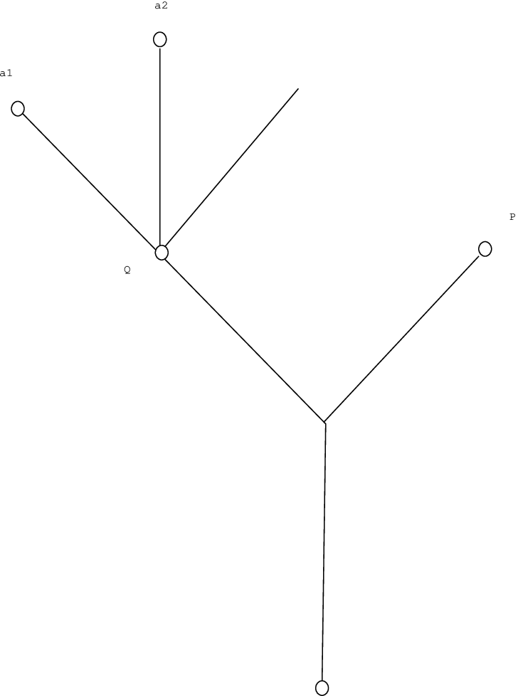
The tree on figure 8 represents an operation which produces the 22-cochain:

a1⊗a2→Q⁡(a1,a2,1)​Pa_{1}\otimes a_{2}\to Q(a_{1},a_{2},1)P

from a degree 00 cochain PP and a degree 33 cochain QQ.

Refer to caption
Figure 8:

Marked vertices in this figure are labeled by small circles. The unmarked terminal vertex corresponds to the insertion of the unit into Q⁡(a1,a2,1)Q(a_{1},a_{2},1) . The unmarked 3-valent vertex gives the product of PP and Q⁡(a1,a2,1)Q(a_{1},a_{2},1) .

Let us denote by ℋmrma​(n,1){\cal H}^{m_{a}}_{m_{r}}(n,1) the set of operations producing a chain in C−mr​(A)C_{-m_{r}}(A) from nn cochains and a chain in C−ma​(A)C_{-m_{a}}(A) .

ℋmrma​(n,1){\cal H}^{m_{a}}_{m_{r}}(n,1) is described using forests of rooted trees drawn on the standard cylinder

Σ=S1×[0,1]{\Sigma}=S^{1}\times[0,1] (4.2)

and subject to the following conditions:

  1. 1.

    every tree of the forest has its root vertex on the boundary S1×{0}S^{1}\times\{0\} ,

  2. 2.

    all vertices of the forest lying on the boundary of the cylinder are marked:

    • •

      the vertices lying on the boundary S1×{1}S^{1}\times\{1\} are marked by integers 0,1,…,ma0,1,\dots,m_{a} in the counterclockwise order; these vertices are reserved for the components of the chain which enters as an argument,

    • •

      the roots are marked by integers 0,1,…,mr0,1,\dots,m_{r} in the same counterclockwise order; they are reserved for components of the resulting chain,

  3. 3.

    all other marked vertices of the forest lie on the lateral surface S1×(0,1)S^{1}\times(0,1) of the cylinder and there are exactly nn such marked vertices.

On the set of these forests we introduce the finest equivalence relation in which two such forests are equivalent if one of them can be obtained from the other by either:

  • •

    isotopy, or

  • •

    the contraction of an edge with unmarked ends, or

  • •

    removing an unmarked vertex with only one edge originating from it and joining the two edges adjacent to this vertex into one edge.

ℋmrma​(n,1){\cal H}^{m_{a}}_{m_{r}}(n,1) is the set of the corresponding equivalence classes.

As we see from the conditions, all unmarked vertices lie on the lateral surface S1×(0,1)S^{1}\times(0,1) of the cylinder. As above, these vertices are reserved for operations of 𝐚𝐬𝐬𝐨𝐜{\bf assoc} . The marked vertices lying on the lateral surface S1×(0,1)S^{1}\times(0,1) are reserved for cochains.

We allow forests with no marked vertices lying on the lateral surface S1×(0,1)S^{1}\times(0,1) . Such forests represent operations which produce a chain from a chain.

Figure 9 gives an example of an operation of ℋ⁡(2,1){\cal H}(2,1) which produces the chain

(b0,b1,b2,b3)=(P​a3,Q⁡(a0,1,a1),1,a2)(b_{0},b_{1},b_{2},b_{3})=(Pa_{3},Q(a_{0},1,a_{1}),1,a_{2}) (4.3)

from a degree 00 cochain PP, a degree 33 cochain QQ and a degree −3-3 chain (a0,a1,a2,a3)(a_{0},a_{1},a_{2},a_{3}) .

Refer to caption
Figure 9: An operation produces which the chain (4.3)

Marked vertices in this figure are labeled by small circles. The unmarked 3-valent vertex gives the product of PP and a3a_{3} , the two unmarked terminal vertices give units of AA and the unmarked 2-valent vertex gives the identity operation on AA . The vertices lying on the boundary S1×{1}S^{1}\times\{1\} are marked by the components of the chain (a0,a1,a2,a3)(a_{0},a_{1},a_{2},a_{3}) and the roots are marked by the components of the chain (4.3).

It is clear how the operad ℋ{\cal H} acts on the pair (C∙​(A),C∙​(A))(C^{\bullet}(A),C_{\bullet}(A)) . From this action it is also clear how to compose the operations. For example, the composition of operations from ℋ⁡(n1,1){\cal H}(n_{1},1) and ℋ⁡(n2,1){\cal H}(n_{2},1) corresponds to putting one cylinder on the top of the other matching the roots of the first cylinder with the vertices lying on the upper circle of the second cylinder, and then shrinking the resulting cylinder to the required height.

Recall that the operad ℋ{\cal H} is colored by degrees of the cochains and degrees of the chains. It is not hard to see that ℋ⁡(n,0){\cal H}(n,0) is a cosimplicial set with respect to the degree of the resulting cochain and a polysimplicial set with respect to the degrees of the cochains entering as arguments.

Similarly, ℋ⁡(n,1){\cal H}(n,1) is a cosimplicial set with respect to the degree of the chain entering as an argument and a polysimplicial set with respect to the degrees of the cochains entering as arguments and the degree of the resulting chain.

These poly-simplicial/cosimplicial structure is compatible with the compositions and we get

Definition 5

The DG operad 𝐊𝐒{\bf KS} is the realization of the operad ℋ{\cal H} in the category of chain complexes.

It follows from the construction that 𝐊𝐒{\bf KS} is a 22-colored operad which acts on the pair (Cnorm∙​(A),C∙norm​(A))(C^{\bullet}_{{\rm norm}}(A),C_{\bullet}^{{\rm norm}}(A)) .

It is not hard to see that the operations ∪\cup (2.24), [,]G[\,,\,]_{G} (2.25), II (2.26), LL (2.27) and BB (2.28) come from the action of the operad 𝐊𝐒{\bf KS} .

Remark 1. The operad 𝐊𝐒{\bf KS} with its action on

(Cnorm∙​(A),C∙norm​(A))(C^{\bullet}_{{\rm norm}}(A),C_{\bullet}^{{\rm norm}}(A))

was introduced by Kontsevich and Soibelman in99 9 See sections 11.1, 11.2, and 11.3 in [23]. [23] in the case when AA is an A∞A_{\infty}-algebra. Here we recall the construction of 𝐊𝐒{\bf KS} in the case when AA is simply an associative algebra. It is this assumption on AA which allows us to utilize the natural cosimplicial/simplicial structure on (Cnorm∙​(A),C∙norm​(A))(C^{\bullet}_{{\rm norm}}(A),C_{\bullet}^{{\rm norm}}(A)) .

Remark 2. If we restrict ourselves to the subspace of operations of 𝐊𝐒{\bf KS} which do not involve chains then we get the minimal operad of Kontsevich and Soibelman described in [22].

4.2 The operad of little discs on a cylinder

A “topological partner” of 𝐊𝐒{\bf KS} is the operad Cyl{\rm Cyl}\, of discs on a cylinder [23], [29]. As well as the operad of Kontsevich and Soibelman Cyl{\rm Cyl}\, is a 22-colored operad satisfying the property (2.15).

The spaces Cyl𝔠​(n,0){\rm Cyl}\,^{{\mathfrak{c}}}(n,0), n≥1n\geq 1 are the spaces of the little disc operad.

To introduce the space Cyl𝔞​(n,1){\rm Cyl}\,^{{\mathfrak{a}}}(n,1) for n≥1n\geq 1 we consider cylinders S1×[a,c]S^{1}\times[a,c] for a,c∈ℝa,c\in{\mathbb{R}}, a<ca<c with the natural flat metric and define the topological space Cyl~n\widetilde{\rm Cyl}\,_{n} .

A point of the space Cyl~n\widetilde{\rm Cyl}\,_{n} is a cylinder S1×[a,c]S^{1}\times[a,c] together with a configuration of n≥1n\geq 1 discs on the lateral surface S1×(a,c)S^{1}\times(a,c) and a position of two points bb and tt lying on the boundaries S1×aS^{1}\times{a} and S1×cS^{1}\times{c} , respectively. The topology on the space Cyl~n\widetilde{\rm Cyl}\,_{n} is defined in the obvious way using the flat metric on the cylinder.

The space Cyl~n\widetilde{\rm Cyl}\,_{n} is equipped with a free action of the group S1×ℝS^{1}\times{\mathbb{R}}. The subgroup S1⊂S1×ℝS^{1}\subset S^{1}\times{\mathbb{R}} simultaneously rotates all the cylinders and the subgroup ℝ⊂S1×ℝ{\mathbb{R}}\subset S^{1}\times{\mathbb{R}} acts by parallel shifts

S1×[a,c]→S1×[a+l,c+l],l∈ℝ.S^{1}\times[a,c]\to S^{1}\times[a+l,c+l]\,,\qquad l\in{\mathbb{R}}\,.

The space Cyl𝔞​(n,1){\rm Cyl}\,^{{\mathfrak{a}}}(n,1) for n≥1n\geq 1 of the operad Cyl{\rm Cyl}\, is the quotient

Cyl𝔞​(n,1)=Cyl~n/S1×ℝ.{\rm Cyl}\,^{{\mathfrak{a}}}(n,1)=\widetilde{\rm Cyl}\,_{n}/S^{1}\times{\mathbb{R}}\,. (4.4)

The space Cyl𝔞​(0,1){\rm Cyl}\,^{{\mathfrak{a}}}(0,1) is the space of configurations of two (possibly coinciding) points bb and tt on the circle S1S^{1} considered modulo rotations. Although it is obvious that Cyl𝔞​(0,1){\rm Cyl}\,^{{\mathfrak{a}}}(0,1) is homeomorphic to the circle S1S^{1} we still define Cyl𝔞​(0,1){\rm Cyl}\,^{{\mathfrak{a}}}(0,1) using the configuration space in order to better visualize the operations of the operad.

The insertions of the type

Cyl𝔠​(n,0)×Cyl𝔠​(m,0)→Cyl𝔠​(n+m−1,0){\rm Cyl}\,^{{\mathfrak{c}}}(n,0)\times{\rm Cyl}\,^{{\mathfrak{c}}}(m,0)\to{\rm Cyl}\,^{{\mathfrak{c}}}(n+m-1,0)

are defined in the same as for the operad of little squares. The operations of the type

Cyl𝔠​(n,0)×Cyl𝔞​(m,1)→Cyl𝔞​(n+m−1,1){\rm Cyl}\,^{{\mathfrak{c}}}(n,0)\times{\rm Cyl}\,^{{\mathfrak{a}}}(m,1)\to{\rm Cyl}\,^{{\mathfrak{a}}}(n+m-1,1)

are insertions of the configuration of little discs of Cyl𝔠​(n,0){\rm Cyl}\,^{{\mathfrak{c}}}(n,0) in a little disc on the lateral surface of a cylinder. Finally the operations of the type

Cyl𝔞​(n,1)×Cyl𝔞​(m,1)→Cyl𝔞​(n+m,1){\rm Cyl}\,^{{\mathfrak{a}}}(n,1)\times{\rm Cyl}\,^{{\mathfrak{a}}}(m,1)\to{\rm Cyl}\,^{{\mathfrak{a}}}(n+m,1)

correspond to putting the first cylinder under the second one while the second cylinder is rotated in such a way that the point bb of the second cylinder coincides with the point tt of the first cylinder. The composition involving degenerate configurations of Cyl𝔞​(0,1){\rm Cyl}\,^{{\mathfrak{a}}}(0,1) are defined in the obvious way.

To describe the operad of homology groups of Cyl{\rm Cyl}\, we will need some results about the configuration spaces of distinct points on the punctured plane ℝ2∖{𝟎}{\mathbb{R}}^{2}\setminus\{{\bf 0}\} .

Let us denote by Confn​(ℝ2∖{𝟎}){\rm Conf}\,_{n}({\mathbb{R}}^{2}\setminus\{{\bf 0}\}) the configuration space of nn distinct points on the punctured plane ℝ2∖{𝟎}{\mathbb{R}}^{2}\setminus\{{\bf 0}\} and consider the following projections

pk:Confn​(ℝ2∖{𝟎})→ℝ2∖{𝟎},p_{k}:{\rm Conf}\,_{n}({\mathbb{R}}^{2}\setminus\{{\bf 0}\})\to{\mathbb{R}}^{2}\setminus\{{\bf 0}\}\,, (4.5)
pk​(𝐱1,…,𝐱n)=𝐱k.p_{k}({\bf x}_{1},\dots,{\bf x}_{n})={\bf x}_{k}\,.

Due to E. Fadell and L. Neuwirth [14] we have

Theorem 1 (Theorem 1, [14])

For every k=1,2,…,nk=1,2,\dots,n the map pkp_{k} is a locally trivial fibration.

Using the ideas of E. Fadell and L. Neuwirth [14] we show that

Proposition 6

The map

p:Confn​(ℝ2∖{𝟎})→Confn−1​(ℝ2∖{𝟎}),p:{\rm Conf}\,_{n}({\mathbb{R}}^{2}\setminus\{{\bf 0}\})\to{\rm Conf}\,_{n-1}({\mathbb{R}}^{2}\setminus\{{\bf 0}\})\,,
p⁡(𝐱1,𝐱2,…,𝐱n)=(𝐱2,…,𝐱n).p({\bf x}_{1},{\bf x}_{2},\dots,{\bf x}_{n})=({\bf x}_{2},\dots,{\bf x}_{n})\,. (4.6)

is a locally trivial fibration. Furthermore, the fiber FnF_{n} of pp is

Fn=ℝ2∖{𝟎,𝐪2,…,𝐪n},F_{n}={\mathbb{R}}^{2}\setminus\{{\bf 0},{\bf q}_{2},\dots,{\bf q}_{n}\}\,, (4.7)

where 𝐪2,…,𝐪n{\bf q}_{2},\dots,{\bf q}_{n} are n−1n-1 distinct points of the punctured plane ℝ2∖{𝟎}{\mathbb{R}}^{2}\setminus\{{\bf 0}\} .

Proof. For the open unit disc D1D_{1} on ℝ2{\mathbb{R}}^{2} centered at the origin there exists a continuous map

θ:D1×D¯1→D¯1\theta:D_{1}\times\bar{D}_{1}\to\bar{D}_{1} (4.8)

satisfying the following properties:

– for all 𝐱∈D1{\bf x}\in D_{1} the map θ(𝐱,):D¯1→D¯1\theta({\bf x},\,\,):\bar{D}_{1}\to\bar{D}_{1} is a a homeomorphism having ∂D¯1{\partial}\bar{D}_{1} fixed.

– for all 𝐱∈D1{\bf x}\in D_{1} we have θ⁡(𝐱,𝐱)=𝟎\theta({\bf x},{\bf x})={\bf 0} .

For distinct points 𝐪2,…,𝐪n{\bf q}_{2},\dots,{\bf q}_{n} on the punctured plane ℝ2∖{𝟎}{\mathbb{R}}^{2}\setminus\{{\bf 0}\} we choose open discs

D𝐪2,D𝐪3,…,D𝐪n,D_{{\bf q}_{2}},\,D_{{\bf q}_{3}},\,\dots,\,D_{{\bf q}_{n}}\,, (4.9)

which are centered at 𝐪2,𝐪3,…,𝐪n{\bf q}_{2},{\bf q}_{3},\dots,{\bf q}_{n}, respectively. Each disc D¯𝐪j\bar{D}_{{\bf q}_{j}} avoids the origin 𝟎{\bf 0} and for each i≠ji\neq j

D¯𝐪i∩D¯𝐪j=∅.\bar{D}_{{\bf q}_{i}}\cap\bar{D}_{{\bf q}_{j}}=\emptyset\,.

Let us denote respectively by r2,…,rnr_{2},\dots,r_{n} the radii of the discs (4.9) and let UbU_{b} be the following neighborhood of Confn−1​(ℝ2∖{𝟎}){\rm Conf}\,_{n-1}({\mathbb{R}}^{2}\setminus\{\bf 0\}):

Ub={(𝐱2,…,𝐱n)|𝐱2∈D𝐪2,𝐱3∈D𝐪3,…,𝐱n∈D𝐪n}.U_{b}=\{({\bf x}_{2},\dots,{\bf x}_{n})\,\,|\,\,{\bf x}_{2}\in D_{{\bf q}_{2}}\,,\quad{\bf x}_{3}\in D_{{\bf q}_{3}}\,,\,\dots\,,{\bf x}_{n}\in D_{{\bf q}_{n}}\}\,. (4.10)

The desired homeomorphism hh from p−1​(Ub)→Fn×Ubp^{-1}(U_{b})\to F_{n}\times U_{b} is given by the formula:

h⁡(𝐱1,𝐱2,…,𝐱n)={(𝐱1,𝐱2,…,𝐱n),if​𝐱1∉⋃j=2nD𝐪j,(𝐪j+rj​θ​(𝐱j−𝐪jrj,𝐱1−𝐪jrj),𝐱2,…,𝐱n),if​𝐱1∈D¯𝐪j,h({\bf x}_{1},{\bf x}_{2},\dots,{\bf x}_{n})=\begin{cases}\displaystyle({\bf x}_{1},{\bf x}_{2},\dots,{\bf x}_{n})\,,\qquad{\rm if}~~{\bf x}_{1}\notin\bigcup_{j=2}^{n}D_{{\bf q}_{j}}\,,\\[8.5359pt] \displaystyle({\bf q}_{j}+r_{j}\,\theta\Big(\frac{{\bf x}_{j}-{\bf q}_{j}}{r_{j}},\frac{{\bf x}_{1}-{\bf q}_{j}}{r_{j}}\Big),{\bf x}_{2},\dots,{\bf x}_{n})\,,\quad{\rm if}~~{\bf x}_{1}\in\bar{D}_{{\bf q}_{j}}\,,\end{cases} (4.11)

where rjr_{j} is the radius of the jj-th disc D𝐪jD_{{\bf q}_{j}} .

Since the open subsets of the form UbU_{b} (4.10) cover Confn−1​(ℝ2∖{𝟎}){\rm Conf}\,_{n-1}({\mathbb{R}}^{2}\setminus\{\bf 0\}) the map pp (4.6) is indeed a locally trivial fibration. □\Box

Fiber FnF_{n} of pp (4.6) is homotopy equivalent to the wedge sum ∨nS1\vee^{n}S^{1} of nn circles. Hence, the homology groups of FnF_{n} (4.7) are

H∙​(Fn,𝕂)={𝕂,if∙=0,𝕂n,if∙=1,0,otherwise.H_{{\bullet}}(F_{n},{\mathbb{K}})=\begin{cases}{\mathbb{K}}\,,\qquad{\rm if}~~{\bullet}=0\,,\\ {\mathbb{K}}^{n}\,,\qquad{\rm if}~~{\bullet}=1\,,\\ 0\,,\qquad{\rm otherwise}\,.\end{cases} (4.12)

Let us show that

Proposition 7

The fundamental group π1​(Confn−1​(ℝ2∖{𝟎}))\pi_{1}({\rm Conf}\,_{n-1}({\mathbb{R}}^{2}\setminus\{\bf 0\})) acts trivially on the homology groups H∙​(Fn,𝕂)H_{{\bullet}}(F_{n},{\mathbb{K}}) of FnF_{n} .

Proof. It is obvious that we only need to consider the action of π1​(Confn−1​(ℝ2∖{𝟎}))\pi_{1}({\rm Conf}\,_{n-1}({\mathbb{R}}^{2}\setminus\{\bf 0\})) on H1​(Fn,𝕂)H_{1}(F_{n},{\mathbb{K}}) .

To get the cycles representing elements of a basis for H1​(Fn,𝕂)H_{1}(F_{n},{\mathbb{K}}) we choose closed discs

D𝟎,D𝐪2,D𝐪3,…,D𝐪n,D_{\bf 0},\,D_{{\bf q}_{2}},\,D_{{\bf q}_{3}},\,\dots,\,D_{{\bf q}_{n}}\,, (4.13)

which are centered at 𝟎,𝐪2,𝐪3,…,𝐪n{\bf 0},{\bf q}_{2},{\bf q}_{3},\dots,{\bf q}_{n}, respectively. The discs (4.13) are chosen in such a way that their closures

D¯𝟎,D¯𝐪2,D¯𝐪3,…,D¯𝐪n\bar{D}_{\bf 0},\,\bar{D}_{{\bf q}_{2}},\,\bar{D}_{{\bf q}_{3}},\,\dots,\,\bar{D}_{{\bf q}_{n}}

are pairwise disjoint.

The boundaries of the discs (4.13) are cycles representing the elements of a basis for H1​(Fn,𝕂)H_{1}(F_{n},{\mathbb{K}}) .

Let us identify ℝ2{\mathbb{R}}^{2} with the complex plane ℂ{\mathbb{C}} and consider the following loop in Confn−1​(ℝ2∖{𝟎}){\rm Conf}\,_{n-1}({\mathbb{R}}^{2}\setminus\{\bf 0\})

f⁡(t)=(e2​π​i​t​𝐪2,e2​π​i​t​𝐪3,…,e2​π​i​t​𝐪n):[0,1]→Confn−1​(ℝ2∖{𝟎}),f(t)=(e^{2\pi it}{\bf q}_{2},e^{2\pi it}{\bf q}_{3},\dots,e^{2\pi it}{\bf q}_{n})\,:\,[0,1]\to{\rm Conf}\,_{n-1}({\mathbb{R}}^{2}\setminus\{\bf 0\})\,, (4.14)

where (𝐪2,𝐪3,…,𝐪n)({\bf q}_{2},{\bf q}_{3},\dots,{\bf q}_{n}) is a fixed collection of the distinct points of ℝ2∖{𝟎}{\mathbb{R}}^{2}\setminus\{\bf 0\} .

The loop (4.14) lifts to the following loop in Confn​(ℝ2∖{𝟎}){\rm Conf}\,_{n}({\mathbb{R}}^{2}\setminus\{\bf 0\})

f~​(t)=(e2​π​i​t​𝐱1,e2​π​i​t​𝐪2,e2​π​i​t​𝐪3,…,e2​π​i​t​𝐪n):[0,1]→Confn​(ℝ2∖{𝟎}).{\widetilde{f}}(t)=(e^{2\pi it}{\bf x}_{1},e^{2\pi it}{\bf q}_{2},e^{2\pi it}{\bf q}_{3},\dots,e^{2\pi it}{\bf q}_{n})\,:\,[0,1]\to{\rm Conf}\,_{n}({\mathbb{R}}^{2}\setminus\{\bf 0\})\,. (4.15)

As we go around the loop (4.15) the point 𝐱1{\bf x}_{1} of the fiber FnF_{n} returns to its original position. Thus the element [f]∈π1​(Confn−1​(ℝ2∖{𝟎}))[f]\in\pi_{1}({\rm Conf}\,_{n-1}({\mathbb{R}}^{2}\setminus\{\bf 0\})) represented by the loop ff (4.14) acts trivially on H∙​(Fn,𝕂)H_{{\bullet}}(F_{n},{\mathbb{K}}) .

Let now gg be an arbitrary loop in Confn−1​(ℝ2∖{𝟎}){\rm Conf}\,_{n-1}({\mathbb{R}}^{2}\setminus\{\bf 0\}) .

To find the action of the homotopy class [g][g] on H∙​(Fn,𝕂)H_{{\bullet}}(F_{n},{\mathbb{K}}) we need to lift the map

γ⁡(y,t)=g⁡(t):Fn×[0,1]→Confn−1​(ℝ2∖{𝟎}){\gamma}(y,t)=g(t):F_{n}\times[0,1]\to{\rm Conf}\,_{n-1}({\mathbb{R}}^{2}\setminus\{\bf 0\}) (4.16)

to a map

γ~​(y,t):Fn×[0,1]→Confn​(ℝ2∖{𝟎}){\widetilde{\gamma}}(y,t):F_{n}\times[0,1]\to{\rm Conf}\,_{n}({\mathbb{R}}^{2}\setminus\{\bf 0\}) (4.17)

which makes the diagram

Fn×{0}↪Confn​(ℝ2∖{𝟎})↓γ~↗↓pFn×[0,1]→γConfn−1​(ℝ2∖{𝟎})\begin{array}[]{ccc}F_{n}\times\{0\}&\hookrightarrow&{\rm Conf}\,_{n}({\mathbb{R}}^{2}\setminus\{{\bf 0}\})\\[8.5359pt] \downarrow&~{}^{{\widetilde{\gamma}}}\nearrow&\downarrow^{p}\\[8.5359pt] F_{n}\times[0,1]&\stackrel{{\scriptstyle{\gamma}}}{{\rightarrow}}&{\rm Conf}\,_{n-1}({\mathbb{R}}^{2}\setminus\{{\bf 0}\})\end{array} (4.18)

commutative.

To construct the lift γ~{\widetilde{\gamma}} we divide the segment [0,1][0,1] into small enough subsegments [ti,ti+1][t_{i},t_{i+1}] satisfying the property

g⁡([ti,ti+1])⊂V,g([t_{i},t_{i+1}])\subset V\,, (4.19)

where VV is an open subset of Confn−1​(ℝ2∖{𝟎}){\rm Conf}\,_{n-1}({\mathbb{R}}^{2}\setminus\{\bf 0\}) of the form (4.10) . Then each individual lift

γ~|Fn×[ti,ti+1]:Fn×[ti,ti+1]→Confn​(ℝ2∖{𝟎}){\widetilde{\gamma}}\Big|_{F_{n}\times[t_{i},t_{i+1}]}:F_{n}\times[t_{i},t_{i+1}]\to{\rm Conf}\,_{n}({\mathbb{R}}^{2}\setminus\{{\bf 0}\}) (4.20)

can be constructed using the trivialization (4.11).

With this construction in mind we consider the compositions pk∘gp_{k}\circ g of gg with the projections pkp_{k} (4.5) for k∈{2,…,n}k\in\{2,\,\dots,\,n\} . Since the image pk∘g⁡([0,1])p_{k}\circ g([0,1]) of the segment [0,1][0,1] is a compact subset in ℝ2∖{𝟎}{\mathbb{R}}^{2}\setminus\{{\bf 0}\} we may choose the disc D𝟎D_{\bf 0} in such a way that the closure D¯𝟎\bar{D}_{\bf 0} avoids the points of the images pk∘g⁡([0,1])p_{k}\circ g([0,1]) for all k∈{2,…,n}k\in\{2,\,\dots,\,n\} . Therefore the lift γ~{\widetilde{\gamma}} (4.17) can be chosen in such a way that

γ~​(y,t)=y,∀y∈D¯𝟎⊂Fn.{\widetilde{\gamma}}(y,t)=y\,,\qquad\forall~~y\in\bar{D}_{\bf 0}\subset F_{n}\,.

Hence the action of the homotopy class [g][g] on the homology class represented by the boundary of the disc D𝟎D_{\bf 0} is trivial.

Let us examine the loop pk∘gp_{k}\circ g in ℝ2∖{𝟎}{\mathbb{R}}^{2}\setminus\{\bf 0\} more closely.

Since the fundamental group of ℝ2∖{𝟎}{\mathbb{R}}^{2}\setminus\{\bf 0\} is generated by the homotopy class of the loop

l⁡(t)=e2​π​i​t​𝐪k:[0,1]→ℝ2∖{𝟎}l(t)=e^{2\pi it}{\bf q}_{k}:[0,1]\to{\mathbb{R}}^{2}\setminus\{\bf 0\}

around the origin there exists an integer N∈ℤN\in{\mathbb{Z}} such that the loop pk∘(g∗fN)p_{k}\circ(g*f^{N}) is null-homotopic. Here ff is the loop (4.14) in Confn−1​(ℝ2∖{𝟎}){\rm Conf}\,_{n-1}({\mathbb{R}}^{2}\setminus\{\bf 0\}) .

But the class of ff acts trivially on the homology of the fiber FnF_{n} . Therefore, without loss of generality, we may assume that the composition pk∘gp_{k}\circ g is null-homotopic.

Thus, due to Theorem 1 of Fadell and Neuwirth we may further assume that pk∘gp_{k}\circ g is a constant map

pk∘g⁡(t)≡𝐪k.p_{k}\circ g(t)\equiv{\bf q}_{k}\,. (4.21)

In other words, the kk-th point 𝐱k{\bf x}_{k} does not move as we go along the loop gg .

Since for each j≠kj\neq k the image pj∘g⁡([0,1])p_{j}\circ g([0,1]) of the segment [0,1][0,1] is a compact subset in ℝ2∖{𝟎}{\mathbb{R}}^{2}\setminus\{{\bf 0}\} we may choose the disc D𝐪kD_{{\bf q}_{k}} in such a way that the closure D¯𝐪k\bar{D}_{{\bf q}_{k}} avoids the points of the images pj∘g⁡([0,1])p_{j}\circ g([0,1]) for all j≠kj\neq k .

Thus, using the partition of the segment [0,1][0,1] satisfying the property (4.19) and constructing the lift (4.17) using the trivializations of the form (4.11) we see that the lift γ~{\widetilde{\gamma}} can be chosen in such a way that

γ~​(y,t)=y,∀y∈D¯𝐪k⊂Fn.{\widetilde{\gamma}}(y,t)=y\,,\qquad\forall~~y\in\bar{D}_{{\bf q}_{k}}\subset F_{n}\,.

Therefore the action of the homotopy class [g][g] on the homology class represented by the boundary of the disc D𝐪kD_{{\bf q}_{k}} is trivial.

The proposition is proved. □\Box

Generalizing the result of F. R. Cohen [9] we get the following

Theorem 2

The homology operad H−⁣∙​(Cyl,𝕂)H_{-{\bullet}}({\rm Cyl}\,,{\mathbb{K}}) of Cyl{\rm Cyl}\, with the reversed grading is the operad 𝐜𝐚𝐥𝐜{\bf calc} of calculi.

Proof. Since the operad Cyl{\rm Cyl}\, has two colors algebras over H−⁣∙​(Cyl,𝕂)H_{-{\bullet}}({\rm Cyl}\,,{\mathbb{K}}) are pairs of graded vector spaces (𝒱,𝒲)({\cal V},{\cal W}) .

The components Cyl𝔠​(n,0){\rm Cyl}\,^{{\mathfrak{c}}}(n,0) form the operad of little discs. Thus, due to Theorem 1.2 in1010 10 We only need the operations which survive in characteristic zero. [9] 𝒱{\cal V} is a Gerstenhaber algebra.

The space Cyl𝔠​(0,0){\rm Cyl}\,^{{\mathfrak{c}}}(0,0) is empty, the space Cyl𝔠​(1,0){\rm Cyl}\,^{{\mathfrak{c}}}(1,0) is a point and the space Cyl𝔠​(n,0){\rm Cyl}\,^{{\mathfrak{c}}}(n,0) for n>1n>1 is homotopy equivalent to the space Confn​(ℝ2){\rm Conf}\,_{n}({\mathbb{R}}^{2}) of configurations of nn distinct points on ℝ2{\mathbb{R}}^{2} . The map

Cyl𝔠​(n,0)→∼Confn​(ℝ2){\rm Cyl}\,^{{\mathfrak{c}}}(n,0)\stackrel{{\scriptstyle\sim}}{{\to}}{\rm Conf}\,_{n}({\mathbb{R}}^{2}) (4.22)

which establishes the equivalence associates with a configuration of disjoint discs the configuration of their centers.

The space Conf2​(ℝ2){\rm Conf}\,_{2}({\mathbb{R}}^{2}) is, in turn, homotopy equivalent to S1S^{1} . Thus the generator of H0​(S1)H_{0}(S^{1}) represents the commutative product on 𝒱{\cal V} and the generator of H1​(S1)H_{1}(S^{1}) represents the bracket on 𝒱{\cal V} . This bracket has degree −1-1 because we use the reversed grading on the homology groups.

The operations without inputs of color 𝔠{\mathfrak{c}} correspond to homology classes of the space Cyl𝔞​(0,1){\rm Cyl}\,^{{\mathfrak{a}}}(0,1) . Since this space is homeomorphic to the circle S1S^{1} we have

H∙​(Cyl𝔞​(0,1),𝕂)={𝕂,if∙=0,1,0,otherwise.H_{{\bullet}}({\rm Cyl}\,^{{\mathfrak{a}}}(0,1),{\mathbb{K}})=\begin{cases}{\mathbb{K}}\,,\qquad{\rm if}~~{\bullet}=0,1\,,\\ 0\,,\qquad{\rm otherwise}\,.\end{cases}

The generator of H0​(Cyl𝔞​(0,1))H_{0}({\rm Cyl}\,^{{\mathfrak{a}}}(0,1)) corresponds to the identity transformation of 𝒲{\cal W} and the generator δ{\delta} of H1​(Cyl𝔞​(0,1))H_{1}({\rm Cyl}\,^{{\mathfrak{a}}}(0,1)) corresponds to a unary operation on 𝒲{\cal W} . The operation δ{\delta} has degree −1-1 because we use the reversed grading on the homology groups.

The identity

δ2=0{\delta}^{2}=0

follows immediately from the fact that

H2​(Cyl𝔞​(0,1),𝕂)=0.H_{2}({\rm Cyl}\,^{{\mathfrak{a}}}(0,1),{\mathbb{K}})=0\,.

Let us construct a homotopy equivalence between the space Cyl𝔞​(n,1){\rm Cyl}\,^{{\mathfrak{a}}}(n,1) for n≥1n\geq 1 and the space

Confn​(ℝ2∖𝟎)×S1,{\rm Conf}\,_{n}({\mathbb{R}}^{2}\setminus{\bf 0})\times S^{1}\,, (4.23)

where Confn​(ℝ2∖𝟎){\rm Conf}\,_{n}({\mathbb{R}}^{2}\setminus{\bf 0}) is the configuration space of nn distinct points on the punctured plane ℝ2∖𝟎{\mathbb{R}}^{2}\setminus{\bf 0} .

First, we kill the rotation symmetry by fixing the position of the point tt on the upper boundary S1×{c}S^{1}\times\{c\} of the cylinder S1×[a,c]S^{1}\times[a,c] . Second, we kill translation symmetry by setting c=0c=0 .

Next we assign to each configuration of discs on the lateral surface S1×(a,0)S^{1}\times(a,0) the configuration of centers of the discs. In this way we get a homotopy equivalence between the space Cyl𝔞​(n,1){\rm Cyl}\,^{{\mathfrak{a}}}(n,1) and the space

Confn​(S1×(a,0))×S1,{\rm Conf}\,_{n}(S^{1}\times(a,0))\times S^{1}\,, (4.24)

where the points on the factor S1S^{1} correspond to positions of the point bb on S1×{a}S^{1}\times\{a\} .

Finally, using the map

χ:S1×(a,0)→ℝ2∖𝟎,\chi:S^{1}\times(a,0)\to{\mathbb{R}}^{2}\setminus{\bf 0}\,,
χ⁡(φ,y)=(ya−y​cos⁡(φ),ya−y​sin⁡(φ))\chi({\varphi},y)=\Big(\frac{y}{a-y}\cos({\varphi})\,,\,\frac{y}{a-y}\sin({\varphi})\Big)

we get the desired homotopy equivalence

Cyl𝔞​(n,1)≃Confn​(ℝ2∖𝟎)×S1.{\rm Cyl}\,^{{\mathfrak{a}}}(n,1)\simeq{\rm Conf}\,_{n}({\mathbb{R}}^{2}\setminus{\bf 0})\times S^{1}\,. (4.25)

Let us consider the homology groups of Cyl𝔞​(1,1){\rm Cyl}\,^{{\mathfrak{a}}}(1,1) in more details.

The space Cyl𝔞​(1,1){\rm Cyl}\,^{{\mathfrak{a}}}(1,1) is homotopy equivalent to

ℝ2∖𝟎×S1{\mathbb{R}}^{2}\setminus{\bf 0}\,\times\,S^{1}

and the latter space is, in turn, homotopy equivalent to S1×S1S^{1}\times S^{1} . Thus

Cyl𝔞​(1,1)≃S1×S1.{\rm Cyl}\,^{{\mathfrak{a}}}(1,1)\simeq S^{1}\times S^{1}\,. (4.26)

Therefore

H−⁣∙​(Cyl𝔞​(1,1),𝕂)=𝕂⊕𝐬−1​𝕂2⊕𝐬−2​𝕂.H_{-{\bullet}}({\rm Cyl}\,^{{\mathfrak{a}}}(1,1),{\mathbb{K}})={\mathbb{K}}\oplus{\bf s}\,^{-1}{\mathbb{K}}^{2}\oplus{\bf s}\,^{-2}{\mathbb{K}}\,.

To identify the cycles representing the homology classes we parameterize the circle S1S^{1} by the angle variable φ∈[0,2​π]{\varphi}\in[0,2\pi] and the torus S1×S1S^{1}\times S^{1} by the pair of angle variables φ1,φ2∈[0,2​π]{\varphi}_{1},{\varphi}_{2}\in[0,2\pi] .

The zeroth homology space H0​(Cyl𝔞​(1,1),𝕂)H_{0}({\rm Cyl}\,^{{\mathfrak{a}}}(1,1),{\mathbb{K}}) is one-dimensional and its generator corresponds to the contraction ii of elements of 𝒱{\cal V} with elements of 𝒲{\cal W} . The second homology space H2​(Cyl𝔞​(1,1),𝕂)H_{2}({\rm Cyl}\,^{{\mathfrak{a}}}(1,1),{\mathbb{K}}) is also one-dimensional. Its generator corresponds to the composition δ​i​δ{\delta}\,i\,{\delta} .

The cycle

φ→(0,φ):S1↪S1×S1{\varphi}\to(0,{\varphi}):S^{1}\hookrightarrow S^{1}\times S^{1} (4.27)

represents the homology class corresponding to the composition i​δi\,{\delta} . In order to get this cycle in Cyl𝔞​(1,1){\rm Cyl}\,^{{\mathfrak{a}}}(1,1) we need to revolve the point bb on the lower boundary about the vertical axis as it is shown on Figure 10 .

Refer to caption
Figure 10: How to get the cycle in Cyl𝔞​(1,1){\rm Cyl}\,^{{\mathfrak{a}}}(1,1) representing the operation i​δi\,{\delta}

The composition δ​i{\delta}i is, in turn, represented by the diagonal

φ→(φ,φ):S1→S1×S1{\varphi}\to({\varphi},{\varphi}):S^{1}\to S^{1}\times S^{1} (4.28)

of the torus. To get this cycle we need to revolve simultaneously the disc and the point bb about the vertical axis as it is shown on Figure 11 .

Refer to caption
Figure 11: How to get the cycle in Cyl𝔞​(1,1){\rm Cyl}\,^{{\mathfrak{a}}}(1,1) representing the operation δ​i{\delta}\,i

The homology classes δ​i{\delta}i and i​δi{\delta} form a basis of H1​(Cyl𝔞​(1,1),𝕂)H_{1}({\rm Cyl}\,^{{\mathfrak{a}}}(1,1),{\mathbb{K}}) .

We would like to remark that the homology class represented by the cycle

φ→(φ,0):S1↪S1×S1{\varphi}\to({\varphi},0):S^{1}\hookrightarrow S^{1}\times S^{1} (4.29)

equals to the combination

δ​i−i​δ.{\delta}\,i-i\,{\delta}\,.

Indeed it is easy to see that the cycles (4.27), (4.28), and (4.29) form the boundary of the following 22-simplex in S1×S1S^{1}\times S^{1}

{(φ1,φ2)|φ1≤φ2}⊂S1×S1.\{({\varphi}_{1},{\varphi}_{2})\,\,|\,\,{\varphi}_{1}\leq{\varphi}_{2}\}\subset S^{1}\times S^{1}\,.

Thus the cycle (4.29) represents the homology class corresponding to the Lie derivative ll . To get this cycle in Cyl𝔞​(1,1){\rm Cyl}\,^{{\mathfrak{a}}}(1,1) we need to revolve the disc about the vertical axis as it is shown on Figure 12 .

Refer to caption
Figure 12: How to get the cycle in Cyl𝔞​(1,1){\rm Cyl}\,^{{\mathfrak{a}}}(1,1) representing the operation ll

In general, for n≥1n\geq 1 the homology of the space Cyl𝔞​(n,1){\rm Cyl}\,^{{\mathfrak{a}}}(n,1) can be computed with the help of the homological version of Lemma 6.2 from [9] . Due to this lemma we have

H∙(Confn(ℝ2∖𝟎),𝕂)=⨂j=1nH∙(∨jS1,𝕂).H_{{\bullet}}({\rm Conf}\,_{n}({\mathbb{R}}^{2}\setminus{\bf 0}),{\mathbb{K}})=\bigotimes_{j=1}^{n}H_{{\bullet}}(\vee^{j}\,S^{1},{\mathbb{K}})\,. (4.30)

Using the homotopy equivalence (4.25) and the Künneth formula, we deduce that

H∙(Cyl𝔞(n,1),𝕂)=⨂j=1nH∙(∨jS1,𝕂)⊗H∙(S1,𝕂).H_{{\bullet}}({\rm Cyl}\,^{{\mathfrak{a}}}(n,1),{\mathbb{K}})=\bigotimes_{j=1}^{n}H_{{\bullet}}(\vee^{j}\,S^{1},{\mathbb{K}})\,\,\otimes\,\,H_{{\bullet}}(S^{1},{\mathbb{K}})\,. (4.31)

Let us show that the operad H−⁣∙​(Cyl,𝕂)H_{-{\bullet}}({\rm Cyl}\,,{\mathbb{K}}) is generated by operations of H−⁣∙​(Cyl𝔠​(2,0),𝕂)H_{-{\bullet}}({\rm Cyl}\,^{{\mathfrak{c}}}(2,0),{\mathbb{K}}), H−⁣∙​(Cyl𝔞​(0,1)CLOSEH_{-{\bullet}}({\rm Cyl}\,^{{\mathfrak{a}}}(0,1) , and H−⁣∙​(Cyl𝔞​(1,1),𝕂)H_{-{\bullet}}({\rm Cyl}\,^{{\mathfrak{a}}}(1,1),{\mathbb{K}}) .

Since the case of the operad of little discs was already considered by F. Cohen [9] we should only consider the operations of H−⁣∙​(Cyl𝔞​(n,1),𝕂)H_{-{\bullet}}({\rm Cyl}\,^{{\mathfrak{a}}}(n,1),{\mathbb{K}}) .

Due to homotopy equivalence (4.25) the homology classes of Cyl𝔞​(n,1){\rm Cyl}\,^{{\mathfrak{a}}}(n,1) are of the forms

α⊗1,{\alpha}\otimes 1\,, (4.32)

and

α⊗ϕ,{\alpha}\otimes\phi\,, (4.33)

where α∈H−⁣∙​(Confn​(ℝ2∖𝟎),𝕂){\alpha}\in H_{-{\bullet}}({\rm Conf}\,_{n}({\mathbb{R}}^{2}\setminus{\bf 0}),{\mathbb{K}}) , 11 is the generator of H0​(S1,𝕂)H_{0}(S^{1},{\mathbb{K}}) and ϕ\phi is the generator of H0​(S1,𝕂)H_{0}(S^{1},{\mathbb{K}}) .

It is obvious that homology classes of the form (4.33) are obtained by composing the homology classes of the form (4.32) with the generator δ{\delta} of H1​(Cyl𝔞​(0,1),𝕂)H_{1}({\rm Cyl}\,^{{\mathfrak{a}}}(0,1),{\mathbb{K}}) .

To analyze the homology classes (4.32) we consider the Serre spectral sequence corresponding to the fibration (4.6). Due to Proposition 7 the E2E^{2} term of the sequence is

Ep,q2=Hp​(Confn−1​(ℝ2∖𝟎),𝕂)⊗Hq​(Fn,𝕂),E^{2}_{p,q}=H_{p}({\rm Conf}\,_{n-1}({\mathbb{R}}^{2}\setminus{\bf 0}),{\mathbb{K}})\otimes H_{q}(F_{n},{\mathbb{K}})\,, (4.34)

where FnF_{n} is the fiber (4.7) of pp .

Since FnF_{n} is homotopy equivalent to the wedge ∨nS1\vee^{n}S^{1} of nn circles equation (4.30) implies that the vector spaces

⨁pE2p,∙−p\bigoplus_{p}E^{2}_{p,{\bullet}-p}

and H∙​(Confn​(ℝ2∖𝟎),𝕂)H_{{\bullet}}({\rm Conf}\,_{n}({\mathbb{R}}^{2}\setminus{\bf 0}),{\mathbb{K}}) have the same dimension. Thus, using the fact that spectral sequence corresponding to the fibration (4.6) converges to H∙​(Confn​(ℝ2∖𝟎),𝕂)H_{{\bullet}}({\rm Conf}\,_{n}({\mathbb{R}}^{2}\setminus{\bf 0}),{\mathbb{K}}) , we deduce that this spectral sequence degenerates at E2E_{2} and

H∙(Confn(ℝ2∖𝟎),𝕂)=⨁p+q=∙Hp(Confn−1(ℝ2∖𝟎),𝕂)⊗Hq(Fn,𝕂)H_{{\bullet}}({\rm Conf}\,_{n}({\mathbb{R}}^{2}\setminus{\bf 0}),{\mathbb{K}})=\bigoplus_{p+q={\bullet}}H_{p}({\rm Conf}\,_{n-1}({\mathbb{R}}^{2}\setminus{\bf 0}),{\mathbb{K}})\otimes H_{q}(F_{n},{\mathbb{K}}) (4.35)

Using equation (4.12) we reduce this expression further to

H∙​(Confn​(ℝ2∖𝟎),𝕂)=H_{{\bullet}}({\rm Conf}\,_{n}({\mathbb{R}}^{2}\setminus{\bf 0}),{\mathbb{K}})=
H∙​(Confn−1​(ℝ2∖𝟎),𝕂)⊗H0​(Fn,𝕂)⊕H∙−1​(Confn−1​(ℝ2∖𝟎),𝕂)⊗H1​(Fn,𝕂).H_{{\bullet}}({\rm Conf}\,_{n-1}({\mathbb{R}}^{2}\setminus{\bf 0}),{\mathbb{K}})\otimes H_{0}(F_{n},{\mathbb{K}})\,\,\oplus\,\,H_{{\bullet}-1}({\rm Conf}\,_{n-1}({\mathbb{R}}^{2}\setminus{\bf 0}),{\mathbb{K}})\otimes H_{1}(F_{n},{\mathbb{K}})\,. (4.36)

Let v1,v2,…,vn∈𝒱v_{1},v_{2},\dots,v_{n}\in{\cal V} and w∈𝒲w\in{\cal W} be the arguments of an operation corresponding to a homology class in (4.36). It is not hard to see that the generator of H0​(Fn,𝕂)=𝕂H_{0}(F_{n},{\mathbb{K}})={\mathbb{K}} corresponds to the contraction ii with v1v_{1} and the generators of H1​(Fn,𝕂)=𝕂nH_{1}(F_{n},{\mathbb{K}})={\mathbb{K}}^{n} correspond1111 11 This picture is very reminiscent of the consideration of Hochschild-Serre spectral sequence in the proof of Proposition 4.1 in [28]. to the brackets [v1,vj][v_{1},v_{j}] for j∈{2,3,…,n}j\in\{2,3,\dots,n\} and the Lie derivative lv1l_{v_{1}} along v1v_{1} .

Thus the homology classes of H−⁣∙​(Cyl𝔞​(n,1),𝕂)H_{-{\bullet}}({\rm Cyl}\,^{{\mathfrak{a}}}(n,1),{\mathbb{K}}) are all produced by the operadic compositions of the classes in H−⁣∙​(Cyl𝔞​(n−1,1),𝕂)H_{-{\bullet}}({\rm Cyl}\,^{{\mathfrak{a}}}(n-1,1),{\mathbb{K}}) , H−⁣∙​(Cyl𝔞​(1,1),𝕂)H_{-{\bullet}}({\rm Cyl}\,^{{\mathfrak{a}}}(1,1),{\mathbb{K}}) , and H−⁣∙​(Cyl𝔠​(2,0),𝕂)H_{-{\bullet}}({\rm Cyl}\,^{{\mathfrak{c}}}(2,0),{\mathbb{K}}) .

This inductive argument allows us to conclude that the operad H−⁣∙​(Cyl,𝕂)H_{-{\bullet}}({\rm Cyl}\,,{\mathbb{K}}) is generated by the classes

i∈H0​(Cyl𝔞​(1,1),𝕂),l∈H1​(Cyl𝔞​(1,1),𝕂),δ∈H1​(Cyl𝔞​(0,1),𝕂),∧∈H0(Cyl𝔠(2,0),𝕂),[,]∈H1(Cyl𝔠(2,0),𝕂).\begin{array}[]{c}\begin{array}[]{ccc}i\in H_{0}({\rm Cyl}\,^{{\mathfrak{a}}}(1,1),{\mathbb{K}})\,,&l\in H_{1}({\rm Cyl}\,^{{\mathfrak{a}}}(1,1),{\mathbb{K}})\,,&{\delta}\in H_{1}({\rm Cyl}\,^{{\mathfrak{a}}}(0,1),{\mathbb{K}})\,,\end{array}\\[14.22636pt] \begin{array}[]{cc}\wedge\in H_{0}({\rm Cyl}\,^{{\mathfrak{c}}}(2,0),{\mathbb{K}})\,,&[\,,\,]\in H_{1}({\rm Cyl}\,^{{\mathfrak{c}}}(2,0),{\mathbb{K}})\,.\end{array}\end{array} (4.37)

Using equation (2.23) and the fact [21] that dim𝐋𝐢𝐞⁡(n)=(n−1)!\dim{\bf Lie}(n)=(n-1)! it is not hard to show that

𝐜𝐚𝐥𝐜𝔞​(n,1)≅𝐜𝐚𝐥𝐜𝔞​(n−1,1)⊗(𝕂⊕𝐬−1​𝕂n){\bf calc}^{{\mathfrak{a}}}(n,1)\cong{\bf calc}^{{\mathfrak{a}}}(n-1,1)\otimes({\mathbb{K}}\oplus{\bf s}\,^{-1}{\mathbb{K}}^{n})

as graded vector spaces.

On the other hand, equation (4.31) gives us the same isomorphism

H−⁣∙​(Cyl𝔞​(n,1),𝕂)≅H−⁣∙​(Cyl𝔞​(n−1,1),𝕂)⊗(𝕂⊕𝐬−1​𝕂n)H_{-{\bullet}}({\rm Cyl}\,^{{\mathfrak{a}}}(n,1),{\mathbb{K}})\cong H_{-{\bullet}}({\rm Cyl}\,^{{\mathfrak{a}}}(n-1,1),{\mathbb{K}})\otimes({\mathbb{K}}\oplus{\bf s}\,^{-1}{\mathbb{K}}^{n})

of graded vector spaces for H−⁣∙​(Cyl,𝕂)H_{-{\bullet}}({\rm Cyl}\,,{\mathbb{K}}) .

Therefore, the dimensions of graded components of H−⁣∙​(Cyl𝔞​(n,1),𝕂)H_{-{\bullet}}({\rm Cyl}\,^{{\mathfrak{a}}}(n,1),{\mathbb{K}}) and 𝐜𝐚𝐥𝐜𝔞​(n,1){\bf calc}^{{\mathfrak{a}}}(n,1) are equal.

Thus, in order the complete the proof of the theorem, we need to show the operations (4.37) satisfy the identities of calculus algebra (see Definition 3).

The identities of the Gerstenhaber algebra were already checked in [9]. The identity (2.19) was checked above. On Figure 13

Refer to caption
Figure 13: How to check identity (4.38)

we show how to check the identity

[i,l]=i[,].[i,l]=i_{[\,,\,]}\,. (4.38)

The remaining identities can be checked in the similar way.

Theorem 2 is proved. □\Box

4.3 Required results from [23]

We will need

Theorem 3 (M. Kontsevich, Y. Soibelman, [23])

The operad 𝐊𝐒{\bf KS} is quasi-isomorphic to the operad of singular chains of the topological operad Cyl{\rm Cyl}\,. The homology operad H−⁣∙​(𝐊𝐒,𝕂)H_{-{\bullet}}({\bf KS},{\mathbb{K}}) is generated by the classes of the operations ∪\cup (2.24), [,]G[\,,\,]_{G} (2.25), II (2.26), LL (2.27) and BB (2.28) .

Furthermore, (See Proposition 11.3.3 on page 50 in [23])

Proposition 8

The operad of singular chains of the topological operad Cyl{\rm Cyl}\, is formal.

Combining these two statements with Theorem 2 we get the following corollary.

Corollary 1

The pair (Cnorm∙​(A),C∙norm​(A))(C^{\bullet}_{{\rm norm}}(A),C_{\bullet}^{{\rm norm}}(A)) is a homotopy calculus algebra. The operations of this algebra structure are expressed in terms of operations of ℋ{\cal H} . The induced calculus structure on the pair (H​H∙​(A),H​H∙​(A))(HH^{{\bullet}}(A),HH_{{\bullet}}(A)) coincides with the one in [11] .

4.4 A useful property of the operad 𝐊𝐒{\bf KS}

For the 22-colored operad 𝐊𝐒{\bf KS} of chain complexes we have the following

Proposition 9

The elements of 𝐊𝐒𝔠​(k,0){\bf KS}^{{\mathfrak{c}}}(k,0) have degrees

deg≥1−k\deg\geq 1-k (4.39)

and the elements of 𝐊𝐒𝔞​(k,1){\bf KS}^{{\mathfrak{a}}}(k,1) have degrees

deg≥−1−k.\deg\geq-1-k\,. (4.40)

Proof. Let us start with 𝐊𝐒𝔠​(k,0){\bf KS}^{{\mathfrak{c}}}(k,0) for k=1k=1 . Operations of 𝐊𝐒𝔠​(1,0){\bf KS}^{{\mathfrak{c}}}(1,0) produce a Hochschild cochain from a Hochschild cochain. In order to prove that these operations have nonnegative degrees we need to show that the operations from ℋ⁡(1,0){\cal H}(1,0) which lower the number the number of arguments of the cochain do not contribute to the realization of ℋ{\cal H} .

Let TT be a tree representing an operation from ℋ⁡(1,0){\cal H}(1,0) and let vav_{a} be the vertex adjacent to the root. If vav_{a} is marked then it is marked by the only cochain PP which enters as an argument. All other marked vertices are necessarily terminal and they are reserved for the arguments of the cochain produced by the operation.

In order to lower the number of arguments, we need to insert the unit into the cochain PP. The insertion of the unit is a degeneracy of the simplicial structure on ℋ⁡(1,0){\cal H}(1,0) . Hence all operations from ℋ⁡(1,0){\cal H}(1,0) which lower the degree of the cochain do not contribute to the realization.

If vav_{a} is unmarked then, starting with the marked vertex vPv_{P} reserved for the cochain PP, we can form the proper maximal subtree with vPv_{P} being the vertex adjacent to the root. In order to contribute to the realization the operation corresponding to this subtree has to have a nonnegative degree. Hence, so does the operation corresponding to the whole tree.

We proved (4.39) for k=1k=1 .

Let us take it as a base of the induction and assume that (4.39) is proved for all m<km<k .

We consider a tree TT which represents an operation from ℋ⁡(k,0){\cal H}(k,0) and denote the vertex adjacent to the root of TT by vav_{a} . Let us consider the case when the vertex vav_{a} is marked. Say, vav_{a} is reserved for a cochain P1P_{1} of degree q1q_{1} .

Then the tree TT has exactly q1q_{1} maximal proper subtrees whose root vertex is vav_{a} . We denote these subtrees by T1,T2,…,Tq1T_{1},T_{2},\dots,T_{q_{1}} . The number q1q_{1} splits into the sum

q1=pn+py,q_{1}=p_{n}+p_{y}\,, (4.41)

where pnp_{n} is the number of the subtrees with no vertices reserved for cochains and pyp_{y} is the number of the subtrees in which at least one vertex is reserved for a cochain.

Let PP denote the cochain produced by the operation in question and let rr by the number of arguments of this cochain. We will find an estimate for rr using the inductive assumption.

Every subtree with no vertices reserved for cochains has to give at least one argument for the cochain PP. Otherwise, we have to insert the unit as an argument of the cochain P1P_{1} . In this case the operation in question is a obtained from another operation by degeneracy. Therefore this operation would not contribute to the realization of ℋ{\cal H} .

If TjT_{j} is a subtree with exactly kjk_{j} vertices reserved for cochains then, obviously, kj<kk_{j}<k . Hence, applying the assumption of the induction, we get that the number of arguments of PP coming from TjT_{j} is greater or equal

(1−kj)+qj,(1-k_{j})+q_{j}\,,

where qjq_{j} is the total degree of all cochains entering as arguments of the operation corresponding to the subtree TjT_{j} .

Thus the number rr of the arguments of the cochain PP produced by the operation in question can be estimated by

r≥pn+∑j=1py(1−kj+qj).r\geq p_{n}+\sum_{j=1}^{p_{y}}(1-k_{j}+q_{j})\,. (4.42)

This inequality can be rewritten as

r−(pn+py+∑j=1pyqj)≥−∑j=1pykj.r-(\,p_{n}+p_{y}+\sum_{j=1}^{p_{y}}q_{j}\,)\geq-\sum_{j=1}^{p_{y}}k_{j}\,.

Due to equation (4.41) the sum

pn+py+∑j=1pyqjp_{n}+p_{y}+\sum_{j=1}^{p_{y}}q_{j}

is the total degree of all cochains entering as arguments of the operation. Furthermore, since the vertex vav_{a} is reserved for one of the cochains

∑j=1pykj=k−1\sum_{j=1}^{p_{y}}k_{j}=k-1

and the desired inequality (4.39) is proved in this case.

Let us now consider the case when the vertex vav_{a} is unmarked.

The valency of the vertex vav_{a} has to be at least 22 . Otherwise the operation will have the empty set of arguments. If the valency of this vertex is 22 then we remove it using the equivalence transformation.

Thus, without loss of generality, we may assume that the vertex vav_{a} has at least 22 incoming edges. Let us denote by ss the number of these incoming edges and let T1,…,TsT_{1},\dots,T_{s} be the maximal proper subtrees of TT whose root vertex is vav_{a} .

If the vertices reserved for cochains belong to only one of these subtrees TiT_{i} then excising the subtrees TjT_{j} for j≠ij\neq i we get another operation whose degree is less or equal the degree of the original operation. Since in the new tree the unmarked vertex vav_{a} has the valency 22 we may remove this vertex by the corresponding equivalence transformation.

If in this modified tree the vertex adjacent to the root is marked then we deduce the desired inequality to the case considered above.

Otherwise, we should only consider the case when the vertex vav_{a} is unmarked, its valency is at least 33 and each maximal proper subtree TjT_{j} of TT with root vertex vav_{a} has at least one vertex reserved for a cochain.

Let ss be the number of the maximal proper subtrees of TT whose root vertex is vav_{a} . Since the number of these subtrees is greater or equal than 22 therefore every subtree TjT_{j} represents an operation with the number of arguments kj<kk_{j}<k .

Let deg⁡(Tj)\deg(T_{j}) be the degree of the operation corresponding to the jj-th subtree TjT_{j} . Applying the assumption of the induction we get the inequality

deg⁡(Tj)≥1−kj.\deg(T_{j})\geq 1-k_{j}\,. (4.43)

It is clear that the degree deg⁡(T)\deg(T) of the operation corresponding to the tree TT is the sum of degrees of the operations corresponding to the subtrees T1,…,TsT_{1},\dots,T_{s} . Therefore

deg⁡(T)≥∑i=1s(1−ki).\deg(T)\geq\sum_{i=1}^{s}(1-k_{i})\,.

On the other hand ∑i=1ski=k\displaystyle\sum_{i=1}^{s}k_{i}=k . Therefore,

deg⁡(T)≥s−k\deg(T)\geq s-k

and inequality (4.39) follows from the fact that s≥2s\geq 2 .

To prove the second inequality (4.40) we denote by ℋmrma​(k,1){\cal H}^{m_{a}}_{m_{r}}(k,1) the set of operations producing a chain

(b0,b1,…,bmr)(b_{0},b_{1},\dots,b_{m_{r}}) (4.44)

in C−mr​(A)C_{-m_{r}}(A) from kk cochains and a chain

(c0,c1,…,cma)(c_{0},c_{1},\dots,c_{m_{a}}) (4.45)

in C−ma​(A)C_{-m_{a}}(A) .

Let FF be a forest on the cylinder (4.2) representing an operation from ℋmrma​(k,1){\cal H}^{m_{a}}_{m_{r}}(k,1) which contribute to the realization of ℋ⁡(k,1){\cal H}(k,1) . Our purpose is to prove the inequality

−mr≥−ma+q−1−k,-m_{r}\geq-m_{a}+q-1-k\,, (4.46)

where qq is the total degree of all kk cochains of the operation.

This inequality is equivalent to

ma≥mr+q−1−k.m_{a}\geq m_{r}+q-1-k\,. (4.47)

By construction the forest FF has exactly mrm_{r} trees. Let us denote these trees by S1,…,SmrnS_{1},\dots,S_{m^{n}_{r}} , T1,…,TmryT_{1},\dots,T_{m^{y}_{r}} where the trees S1,…,SmrnS_{1},\dots,S_{m^{n}_{r}} have no vertices reserved for cochains and each tree TiT_{i} has at least one vertex reserved for a cochain. Obviously,

mr=mrn+mry.m_{r}=m^{n}_{r}+m^{y}_{r}\,. (4.48)

The roots of the trees S1,…,SmrnS_{1},\dots,S_{m^{n}_{r}} , T1,…,TmryT_{1},\dots,T_{m^{y}_{r}} are marked by components of the chain (4.44). If the root of the tree SiS_{i} is marked by the component bjb_{j} of the for j≠0j\neq 0 then SiS_{i} has to have at least one terminal vertex marked by a component of the chain (4.45). Otherwise we have to insert the unit as the jj-th component of (4.44) for j≠0j\neq 0 . In this case the operation in question is a composition of the another operation and a degeneracy. Hence, this operation would not contribute to the realization of ℋ⁡(k,1){\cal H}(k,1) .

Let us denote by mim_{i} the number of the terminal vertices of the tree TiT_{i} marked by components of the chain (4.45). If the tree TiT_{i} has exactly kik_{i} vertices reserved for the cochains then TiT_{i} represents an operation from ℋ⁡(ki,0){\cal H}(k_{i},0) . Furthermore, if the operation corresponding to the forest FF contributes to the realization then so does the operation corresponding to the tree TiT_{i} . Hence, the number mim_{i} can be estimated using the inequality (4.39)

mi≥qi+1−ki,m_{i}\geq q_{i}+1-k_{i}\,,

where qiq_{i} is the total degree of all cochains of the operation corresponding to the tree TiT_{i} .

Thus we get the following inequality for mam_{a}

ma≥(mrn−1)+∑i=1mry(qi+1−ki),m_{a}\geq(m^{n}_{r}-1)+\sum_{i=1}^{m^{y}_{r}}(q_{i}+1-k_{i})\,, (4.49)

where the first term (mrn−1)(m^{n}_{r}-1) in the right hand side comes from estimate of the number of the marked terminal vertices of the trees S1,…,SmrnS_{1},\dots,S_{m^{n}_{r}} .

Inequality (4.49) can be rewritten as

ma≥mrn+mry+q−1−k,m_{a}\geq m^{n}_{r}+m^{y}_{r}+q-1-k\,, (4.50)

where qq is the total degree of all kk cochains of the operation in question.

Due to equation (4.48) inequality (4.50) coincides exactly with the desired inequality (4.47).

The proposition is proved. □\Box

5 The homotopy calculus on the pair (Cnorm∙​(A),C∙norm​(A))(C^{\bullet}_{{\rm norm}}(A),C_{\bullet}^{{\rm norm}}(A)) .

Since the operad Λ​𝐋𝐢𝐞δ+{\Lambda}{\bf Lie}^{+}_{{\delta}} is a suboperad of 𝐜𝐚𝐥𝐜{\bf calc} , Corollary 1 implies that the pair

(Cnorm∙​(A),C∙norm​(A))(C^{\bullet}_{{\rm norm}}(A),C_{\bullet}^{{\rm norm}}(A))

carries a natural H​o​(Λ​𝐋𝐢𝐞δ+)Ho({\Lambda}{\bf Lie}^{+}_{{\delta}})-algebra structure. In this section we show that the homotopy calculus on (Cnorm∙​(A),C∙norm​(A))(C^{\bullet}_{{\rm norm}}(A),C_{\bullet}^{{\rm norm}}(A)) can be modified in such a way that its H​o​(Λ​𝐋𝐢𝐞δ+)Ho({\Lambda}{\bf Lie}^{+}_{{\delta}})-algebra part becomes the Λ​𝐋𝐢𝐞δ+{\Lambda}{\bf Lie}^{+}_{{\delta}}-algebra structure given by the operations [,]G[\,,\,]_{G} (2.25), LL (2.27), and BB (2.28).

Due to Proposition 2 a homotopy calculus structure on the pair (Cnorm∙​(A),C∙norm​(A))(C^{\bullet}_{{\rm norm}}(A),C_{\bullet}^{{\rm norm}}(A)) is a Maurer-Cartan element

Q∈Coder′​(𝔽𝐁​(Cnorm∙​(A),C∙norm​(A))).Q\in\rm Coder^{\prime}({\mathbb{F}}_{{\bf B}}(C^{\bullet}_{{\rm norm}}(A),C_{\bullet}^{{\rm norm}}(A)))\,. (5.1)

In other words, QQ is a degree 11 coderivation of the coalgebra 𝔽𝐁​(Cnorm∙​(A),C∙norm​(A)){\mathbb{F}}_{{\bf B}}(C^{\bullet}_{{\rm norm}}(A),C_{\bullet}^{{\rm norm}}(A)) satisfying the condition

Q|Cnorm∙​(A)⊕C∙norm​(A)=0,Q\Big|_{C^{\bullet}_{{\rm norm}}(A)\oplus C_{\bullet}^{{\rm norm}}(A)}=0\,,

and the equation

[∂B​a​r+∂H​o​c​h,Q]+Q∘Q=0,[{\partial}^{Bar}+{\partial}^{Hoch},Q]+Q\circ Q=0\,, (5.2)

where Cnorm∙​(A)⊕C∙norm​(A)C^{\bullet}_{{\rm norm}}(A)\oplus C_{\bullet}^{{\rm norm}}(A) is considered as subspace of 𝔽𝐁​(Cnorm∙​(A),C∙norm​(A)){\mathbb{F}}_{{\bf B}}(C^{\bullet}_{{\rm norm}}(A),C_{\bullet}^{{\rm norm}}(A)) via coaugmentation and ∂H​o​c​h{\partial}^{Hoch} is the differential coming from the Hochschild (co)boundary operator on (Cnorm∙​(A),C∙norm​(A))(C^{\bullet}_{{\rm norm}}(A),C_{\bullet}^{{\rm norm}}(A)) .

It is convenient to reserve a notation for the Lie algebra Coder′​(𝔽𝐁​(Cnorm∙​(A),C∙norm​(A)))\rm Coder^{\prime}({\mathbb{F}}_{{\bf B}}(C^{\bullet}_{{\rm norm}}(A),C_{\bullet}^{{\rm norm}}(A)))

𝕃=Coder′​(𝔽𝐁​(Cnorm∙​(A),C∙norm​(A))).{\mathbb{L}}=\rm Coder^{\prime}({\mathbb{F}}_{{\bf B}}(C^{\bullet}_{{\rm norm}}(A),C_{\bullet}^{{\rm norm}}(A)))\,. (5.3)

Proposition 1 implies that the coderivation QQ is uniquely determined by its composition with the corestriction ρ:𝔽𝐁​(Cnorm∙​(A),C∙norm​(A))→Cnorm∙​(A)⊕C∙norm​(A)\rho:{\mathbb{F}}_{{\bf B}}(C^{\bullet}_{{\rm norm}}(A),C_{\bullet}^{{\rm norm}}(A))\to C^{\bullet}_{{\rm norm}}(A)\oplus C_{\bullet}^{{\rm norm}}(A)

q=ρ∘Q:𝔽𝐁​(Cnorm∙​(A),C∙norm​(A))→Cnorm∙​(A)⊕C∙norm​(A),q=\rho\circ Q:{\mathbb{F}}_{{\bf B}}(C^{\bullet}_{{\rm norm}}(A),C_{\bullet}^{{\rm norm}}(A))\to C^{\bullet}_{{\rm norm}}(A)\oplus C_{\bullet}^{{\rm norm}}(A)\,, (5.4)

while equation (5.2) is equivalent to

[∂H​o​c​h,q]+q∘∂B​a​r+q∘Q=0.[{\partial}^{Hoch},q]+q\circ{\partial}^{Bar}+q\circ Q=0\,. (5.5)

The coalgebra 𝔽𝐁​(Cnorm∙​(A),C∙norm​(A)){\mathbb{F}}_{{\bf B}}(C^{\bullet}_{{\rm norm}}(A),C_{\bullet}^{{\rm norm}}(A)) is equipped with a natural increasing filtration1212 12 See Equation (3.11).

Cnorm∙​(A)⊕C∙norm​(A)​[[u]]=ℱ1​𝔽𝐁​(Cnorm∙​(A),C∙norm​(A))⊂ℱ2​𝔽𝐁​(Cnorm∙​(A),C∙norm​(A))⊂…C^{\bullet}_{{\rm norm}}(A)\oplus C_{\bullet}^{{\rm norm}}(A)[[u]]={\cal F}^{1}\,{\mathbb{F}}_{{\bf B}}(C^{\bullet}_{{\rm norm}}(A),C_{\bullet}^{{\rm norm}}(A))\subset{\cal F}^{2}\,{\mathbb{F}}_{{\bf B}}(C^{\bullet}_{{\rm norm}}(A),C_{\bullet}^{{\rm norm}}(A))\subset\dots
ℱm​𝔽𝐁​(Cnorm∙​(A),C∙norm​(A))𝔠=⨁k≤m𝐁𝔠​(k,0)⊗Sk(Cnorm∙​(A))⊗k,ℱm​𝔽𝐁​(Cnorm∙​(A),C∙norm​(A))𝔞=⨁k+1≤m𝐁𝔞​(k,1)⊗Sk(Cnorm∙​(A))⊗k⊗C∙​(A),\begin{array}[]{c}\displaystyle{\cal F}^{m}\,{\mathbb{F}}_{{\bf B}}(C^{\bullet}_{{\rm norm}}(A),C_{\bullet}^{{\rm norm}}(A))_{{\mathfrak{c}}}=\bigoplus_{k\leq m}{\bf B}^{{\mathfrak{c}}}(k,0)\,\otimes_{S_{k}}\,(C^{\bullet}_{{\rm norm}}(A))^{\otimes\,k}\,,\\[8.5359pt] \displaystyle{\cal F}^{m}\,{\mathbb{F}}_{{\bf B}}(C^{\bullet}_{{\rm norm}}(A),C_{\bullet}^{{\rm norm}}(A))_{{\mathfrak{a}}}=\bigoplus_{k+1\leq m}{\bf B}^{{\mathfrak{a}}}(k,1)\,\otimes_{S_{k}}\,(C^{\bullet}_{{\rm norm}}(A))^{\otimes\,k}\otimes C_{\bullet}(A)\,,\end{array} (5.6)

where uu is an auxiliary variable of degree −2-2 .

Using (5.6) we endow the Lie algebra (5.3) with the following decreasing filtration

𝕃=ℱ0​𝕃⊃ℱ1​𝕃⊃ℱ2​𝕃⊃…{\mathbb{L}}={\cal F}^{0}\,{\mathbb{L}}\supset{\cal F}^{1}\,{\mathbb{L}}\supset{\cal F}^{2}\,{\mathbb{L}}\supset\dots
ℱm​𝕃={Y∈𝕃|Y|ℱm​𝔽𝐁​(Cnorm∙​(A),C∙norm​(A))=0}.{\cal F}^{m}\,{\mathbb{L}}=\{\,Y\in{\mathbb{L}}~~|~~Y\Big|_{{\cal F}^{m}\,{\mathbb{F}}_{{\bf B}}(C^{\bullet}_{{\rm norm}}(A),C_{\bullet}^{{\rm norm}}(A))}=0\,\}\,. (5.7)

Since

𝕃=limm𝕃/ℱm​𝕃{\mathbb{L}}=\lim_{m}{\mathbb{L}}/{\cal F}^{m}\,{\mathbb{L}}

the Lie subalgebra ℱ1​𝕃0{\cal F}^{1}{\mathbb{L}}^{0} is pronilpotent.

Therefore ℱ1​𝕃0{\cal F}^{1}{\mathbb{L}}^{0} integrates to a prounipotent group

𝔾=exp⁡(ℱ1​𝕃0){\mathbb{G}}=\exp({\cal F}^{1}{\mathbb{L}}^{0}) (5.8)

which acts on the Maurer-Cartan elements of 𝕃{\mathbb{L}} . This action is defined by the formula:

exp(Y)Q=exp([,Y])Q+f([,Y])[∂B​a​r+∂H​o​c​h,Y],\exp(Y)\,Q=\exp([\,\,,Y])\,Q+f([\,\,,Y])\,[{\partial}^{Bar}+{\partial}^{Hoch},Y]\,, (5.9)

where ff is the power series of the function

f⁡(x)=ex−1xf(x)=\frac{e^{x}-1}{x}

at the point x=0x=0 .

Let QQ be a Maurer-Cartan element of the DGLA 𝕃{\mathbb{L}} which corresponds to the homotopy calculus structure on the pair (Cnorm∙​(A),C∙norm​(A))(C^{\bullet}_{{\rm norm}}(A),C_{\bullet}^{{\rm norm}}(A)) which comes from the action of the operad 𝐊𝐒{\bf KS} .

For every Y∈ℱ1​𝕃Y\in{\cal F}^{1}{\mathbb{L}} the homotopy calculus on the pair (Cnorm∙​(A),C∙norm​(A))(C^{\bullet}_{{\rm norm}}(A),C_{\bullet}^{{\rm norm}}(A)) corresponding to the Maurer-Cartan element exp⁡(Y)​Q\exp(Y)\,Q is quasi-isomorphic to the homotopy calculus corresponding the original Maurer-Cartan element QQ . Indeed, the desired Ho⁡(𝐜𝐚𝐥𝐜){\rm Ho}\,({\bf calc})-quasi-isomorphism is expressed in terms of YY as

exp([,Y]):(𝔽𝐁(Cnorm∙(A),C∙norm(A)),Q)→(𝔽𝐁(Cnorm∙(A),C∙norm(A)),exp(Y)Q).\exp([\,\,,Y]):({\mathbb{F}}_{{\bf B}}(C^{\bullet}_{{\rm norm}}(A),C_{\bullet}^{{\rm norm}}(A)),Q)\to({\mathbb{F}}_{{\bf B}}(C^{\bullet}_{{\rm norm}}(A),C_{\bullet}^{{\rm norm}}(A)),\exp(Y)\,Q)\,. (5.10)

Thus we get a family of mutually quasi-isomorphic homotopy calculus structures on (Cnorm∙​(A),C∙norm​(A))(C^{\bullet}_{{\rm norm}}(A),C_{\bullet}^{{\rm norm}}(A)) . Let us denote this family by 𝐒𝐜𝐚𝐥𝐜{\bf S}_{{\bf calc}} .

We claim that

Theorem 4

The family 𝐒𝐜𝐚𝐥𝐜{\bf S}_{{\bf calc}} contains a homotopy calculus structure whose H​o​(Λ​𝐋𝐢𝐞δ+)Ho({\Lambda}{\bf Lie}^{+}_{{\delta}})-algebra part is the Λ​𝐋𝐢𝐞δ+{\Lambda}{\bf Lie}^{+}_{{\delta}}-algebra structure given by the operations [,]G[\,,\,]_{G} (2.25), LL (2.27), and BB (2.28).

Proof. According to Proposition 2 and equation (3.26) the Ho⁡(Λ​𝐋𝐢𝐞δ+){\rm Ho}\,({\Lambda}{\bf Lie}^{+}_{{\delta}}) is given by a Maurer-Cartan element MM of the DGLA

Coder′​(𝔽Λ​(𝐋𝐢𝐞δ+)∨​(Cnorm∙​(A),C∙norm​(A))).\rm Coder^{\prime}(\,{\mathbb{F}}_{{\Lambda}({\bf Lie}^{+}_{{\delta}})^{\vee}}(C^{\bullet}_{{\rm norm}}(A),C_{\bullet}^{{\rm norm}}(A))\,)\,. (5.11)

Due to Proposition 1 this Maurer-Cartan element is, in turn, uniquely determined by the composition with the corestriction ρ\rho onto Cnorm∙​(A)⊕C∙norm​(A)C^{\bullet}_{{\rm norm}}(A)\oplus C_{\bullet}^{{\rm norm}}(A)

m=ρ∘M:𝔽Λ​(𝐋𝐢𝐞δ+)∨​(Cnorm∙​(A),C∙norm​(A))→Cnorm∙​(A)⊕C∙norm​(A).m=\rho\circ M:{\mathbb{F}}_{{\Lambda}({\bf Lie}^{+}_{{\delta}})^{\vee}}(C^{\bullet}_{{\rm norm}}(A),C_{\bullet}^{{\rm norm}}(A))\to C^{\bullet}_{{\rm norm}}(A)\oplus C_{\bullet}^{{\rm norm}}(A)\,. (5.12)

Finally, Proposition 3 shows that the map mm is related to the map qq (5.4) by the equation

m=q|𝔽Λ​(𝐋𝐢𝐞δ+)∨​(Cnorm∙​(A),C∙norm​(A)),m=q\Big|_{{\mathbb{F}}_{{\Lambda}({\bf Lie}^{+}_{{\delta}})^{\vee}}(C^{\bullet}_{{\rm norm}}(A),C_{\bullet}^{{\rm norm}}(A))}\,, (5.13)

where Λ​(𝐋𝐢𝐞δ+)∨{\Lambda}({\bf Lie}^{+}_{{\delta}})^{\vee} is considered as a sub-cooperad of 𝐁=B​a​r​(𝐜𝐚𝐥𝐜){\bf B}=Bar({\bf calc}) via the chain of embeddings:

Λ​(𝐋𝐢𝐞δ+)∨↪B​a​r​(Λ​𝐋𝐢𝐞δ+)↪B​a​r​(𝐜𝐚𝐥𝐜).{\Lambda}({\bf Lie}^{+}_{{\delta}})^{\vee}\hookrightarrow Bar({\Lambda}{\bf Lie}^{+}_{{\delta}})\hookrightarrow Bar({\bf calc})\,.

The Ho⁡(Λ​𝐋𝐢𝐞){\rm Ho}\,({\Lambda}{\bf Lie})-algebra structure on Cnorm∙​(A)C^{\bullet}_{{\rm norm}}(A) is induced by the Ho⁡(𝐞𝟐){\rm Ho}\,({\bf e_{2}})-algebra structure which, in turn, comes from the action of the minimal operad of Kontsevich and Soibelman [22] on Cnorm∙​(A)C^{\bullet}_{{\rm norm}}(A) . It was proved in [13] (see Theorem 2) that this Ho⁡(𝐋𝐢𝐞){\rm Ho}\,({\bf Lie})-algebra is in fact a genuine Lie algebra given by [,]G[\,,\,]_{G} .

Thus it remains to take care about the operations involving a chain.

Due to (3.27) all the operations of the Ho⁡(Λ​𝐋𝐢𝐞δ+){\rm Ho}\,({\Lambda}{\bf Lie}^{+}_{{\delta}})-algebra involving a chain are combined into a single degree 11 map

m𝔞=m^{{\mathfrak{a}}}=
m|𝔽Λ2​𝐜𝐨𝐜𝐨𝐦𝐦+​(Cnorm∙​(A),C∙norm​(A)​[[u]])𝔞:𝔽Λ2​𝐜𝐨𝐜𝐨𝐦𝐦+​(Cnorm∙​(A),C∙norm​(A)​[[u]])m\Big|_{{\mathbb{F}}_{{\Lambda}^{2}{\bf cocomm}^{+}}(C^{\bullet}_{{\rm norm}}(A),C_{\bullet}^{{\rm norm}}(A)[[u]])_{{\mathfrak{a}}}}:{\mathbb{F}}_{{\Lambda}^{2}{\bf cocomm}^{+}}(C^{\bullet}_{{\rm norm}}(A),C_{\bullet}^{{\rm norm}}(A)[[u]]) (5.14)
→C∙norm​(A).\to C_{\bullet}^{{\rm norm}}(A)\,.

such that

m𝔞|C∙norm​(A)=0.m^{{\mathfrak{a}}}\Big|_{C_{\bullet}^{{\rm norm}}(A)}=0\,. (5.15)

The latter equation follows from the fact that the coderivation MM belongs to the DGLA (5.11).

In other words, we have the infinite collection of operations:

mk,n𝔞:Sk​(Cnorm∙​(A))⊗C∙norm​(A)→C∙norm​(A)m^{{\mathfrak{a}}}_{k,n}:S^{k}(C^{\bullet}_{{\rm norm}}(A))\otimes C_{\bullet}^{{\rm norm}}(A)\to C_{\bullet}^{{\rm norm}}(A) (5.16)

of degrees 1−2​k−2​n1-2k-2n , where Sk​(Cnorm∙​(A))S^{k}(C^{\bullet}_{{\rm norm}}(A)) is the kk-th component of the symmetric algebra S⁡(Cnorm∙​(A))S(C^{\bullet}_{{\rm norm}}(A)) of Cnorm∙​(A)C^{\bullet}_{{\rm norm}}(A) .

Due to Proposition 9 the operation mk,n𝔞m^{{\mathfrak{a}}}_{k,n} vanish if k+2​n>2k+2n>2 . Furthermore, due to equation (5.15) we have m0,0𝔞=0m^{{\mathfrak{a}}}_{0,0}=0 . Thus we need to analyze only there operations: one unary operation

m0,1𝔞:C∙norm​(A)→C∙norm​(A)m^{{\mathfrak{a}}}_{0,1}:C_{\bullet}^{{\rm norm}}(A)\to C_{\bullet}^{{\rm norm}}(A) (5.17)

of degree −1-1 , one binary operation

m1,0𝔞:Cnorm∙​(A)⊗C∙norm​(A)→C∙norm​(A)m^{{\mathfrak{a}}}_{1,0}:C^{\bullet}_{{\rm norm}}(A)\otimes C_{\bullet}^{{\rm norm}}(A)\to C_{\bullet}^{{\rm norm}}(A) (5.18)

of degree −1-1 and one ternary operation

m2,0𝔞:S2​(Cnorm∙​(A))⊗C∙norm​(A)→C∙norm​(A)m^{{\mathfrak{a}}}_{2,0}:S^{2}(C^{\bullet}_{{\rm norm}}(A))\otimes C_{\bullet}^{{\rm norm}}(A)\to C_{\bullet}^{{\rm norm}}(A) (5.19)

of degree −3-3 .

Theorems 2 and 3 imply that the operation (5.17) differs from Connes’ operator BB by an exact operation. Namely,

m0,1𝔞​(c)=B⁡(c)+∂H​o​c​hβ⁡(c)−β⁡(∂H​o​c​hc),m^{{\mathfrak{a}}}_{0,1}(c)=B(c)+{\partial}^{Hoch}\,\beta(c)-\beta({\partial}^{Hoch}\,c)\,,

where β\beta is an operation in 𝐊𝐒{\bf KS}

β:C∙norm​(A)→C∙norm​(A)\beta:C_{\bullet}^{{\rm norm}}(A)\to C_{\bullet}^{{\rm norm}}(A)

of degree −2-2 .

Using Proposition 9 we deduce that β\beta is zero. Hence m0,1𝔞=Bm^{{\mathfrak{a}}}_{0,1}=B .

Due to Proposition 3 the operation (5.18) is expressed in terms of qq (5.4) as

m1,0𝔞​(P,c)=q⁡(b1),m^{{\mathfrak{a}}}_{1,0}(P,c)=q(b_{1})\,, (5.20)

where P∈Cnorm∙​(A)P\in C^{\bullet}_{{\rm norm}}(A) , c∈C∙norm​(A)c\in C_{\bullet}^{{\rm norm}}(A) , and the element b1∈𝔽𝐁​(Cnorm∙​(A),C∙norm​(A))b_{1}\in{\mathbb{F}}_{{\bf B}}(C^{\bullet}_{{\rm norm}}(A),C_{\bullet}^{{\rm norm}}(A)) is depicted on Figure 14.

Theorems 2 and 3 imply that m1,0𝔞m^{{\mathfrak{a}}}_{1,0} differs from the action LL of cochains on chains by an exact operation. In other words,

m1,0𝔞​(P,c)=−(−1)|P|​LP​c+∂H​o​c​hψ⁡(P,c)−ψ⁡(∂H​o​c​hP,c)−(−1)|P|​ψ​(P,∂H​o​c​hc),m^{{\mathfrak{a}}}_{1,0}(P,c)=-(-1)^{|P|}L_{P}\,c+{\partial}^{Hoch}\psi(P,c)-\psi({\partial}^{Hoch}P,c)-(-1)^{|P|}\psi(P,{\partial}^{Hoch}c)\,, (5.21)

where |P||P| is the degree of PP and

ψ:Cnorm∙​(A)⊗C∙norm​(A)→C∙norm​(A)\psi:C^{\bullet}_{{\rm norm}}(A)\otimes C_{\bullet}^{{\rm norm}}(A)\to C_{\bullet}^{{\rm norm}}(A)

is an operation in 𝐊𝐒𝔞​(1,1){\bf KS}^{{\mathfrak{a}}}(1,1) of degree −2-2 .

We remark that ψ\psi may be considered as a map

ψ:Λ​(𝐋𝐢𝐞+)∨​(1,1)⊗Cnorm∙​(A)⊗C∙norm​(A)→C∙norm​(A)\psi:{\Lambda}({\bf Lie}^{+})^{\vee}(1,1)\otimes C^{\bullet}_{{\rm norm}}(A)\otimes C_{\bullet}^{{\rm norm}}(A)\to C_{\bullet}^{{\rm norm}}(A) (5.22)

of degree 00 . Our purpose is to extend ψ\psi “by zero” to the whole vector space of the coalgebra 𝔽𝐁​(Cnorm∙​(A),C∙norm​(A)){\mathbb{F}}_{{\bf B}}(C^{\bullet}_{{\rm norm}}(A),C_{\bullet}^{{\rm norm}}(A)) . This extension depends on the choice of basis in 𝐜𝐚𝐥𝐜𝔞​(1,1){\bf calc}^{{\mathfrak{a}}}(1,1) .

We choose the basis

{l,i,i​δ,l​δ}\{l,~i,~i\,{\delta},~l\,{\delta}\} (5.23)

and extend ψ\psi to 𝐁𝔞​(1,1)⊗Cnorm∙​(A)⊗C∙norm​(A){\bf B}^{{\mathfrak{a}}}(1,1)\otimes C^{\bullet}_{{\rm norm}}(A)\otimes C_{\bullet}^{{\rm norm}}(A)

ψ:𝐁𝔞​(1,1)⊗Cnorm∙​(A)⊗C∙norm​(A)→C∙norm​(A),\psi:{\bf B}^{{\mathfrak{a}}}(1,1)\otimes C^{\bullet}_{{\rm norm}}(A)\otimes C_{\bullet}^{{\rm norm}}(A)\to C_{\bullet}^{{\rm norm}}(A)\,, (5.24)

as

ψ⁡(b1)=ψ⁡(P,c),ψ⁡(b2)=ψ⁡(b3)=ψ⁡(b4)=0,\psi(b_{1})=\psi(P,c)\,,\qquad\psi(b_{2})=\psi(b_{3})=\psi(b_{4})=0\,,
ψ⁡(bλ)=0,\psi(b_{{\lambda}})=0\,,

where the elements

b1,b2,b3,b4,bλ∈𝐁𝔞​(1,1)⊗Cnorm∙​(A)⊗C∙norm​(A)b_{1},b_{2},b_{3},b_{4},b_{{\lambda}}\in{\bf B}^{{\mathfrak{a}}}(1,1)\otimes C^{\bullet}_{{\rm norm}}(A)\otimes C_{\bullet}^{{\rm norm}}(A)

are depicted

Refer to caption
Figure 14: Elements b1b_{1} and b2b_{2}

on Figures 14, 15, 16 ,

Refer to caption
Figure 15: Elements b3b_{3} and b4b_{4}

λ{\lambda} is an arbitrary element of the basis (5.23),

Refer to caption
Figure 16: The number of δ{\delta}’s is ≥1\geq 1

and P∈Cnorm∙​(A)P\in C^{\bullet}_{{\rm norm}}(A) , c∈C∙norm​(A)c\in C_{\bullet}^{{\rm norm}}(A) .

Next we extend ψ\psi by zero to the whole vector space of the coalgebra

𝔽𝐁​(Cnorm∙​(A),C∙norm​(A))=⨁n𝐁𝔠​(n,0)⊗Sn(Cnorm∙​(A))⊗n⊕⨁n𝐁𝔞​(n,1)⊗Sn(Cnorm∙​(A))⊗n⊗C∙norm​(A).\begin{array}[]{c}{\mathbb{F}}_{{\bf B}}(C^{\bullet}_{{\rm norm}}(A),C_{\bullet}^{{\rm norm}}(A))=\\[11.38092pt] \displaystyle\bigoplus_{n}{\bf B}^{{\mathfrak{c}}}(n,0)\otimes_{S_{n}}(C^{\bullet}_{{\rm norm}}(A))^{\otimes\,n}\,\,\oplus\,\,\bigoplus_{n}{\bf B}^{{\mathfrak{a}}}(n,1)\otimes_{S_{n}}(C^{\bullet}_{{\rm norm}}(A))^{\otimes\,n}\otimes C_{\bullet}^{{\rm norm}}(A)\,.\end{array} (5.25)

Then according to Proposition 1 the equation

ρ∘Ψ=ψ\rho\circ\Psi=\psi

defines a derivation Ψ\Psi of the coalgebra (5.25). The derivation Ψ\Psi has degree 00 since so does the map ψ\psi . Furthermore, it is obvious that

Ψ∈ℱ1​𝕃.\Psi\in{\cal F}^{1}\,{\mathbb{L}}\,.

Applying the element exp⁡(−Ψ)\exp(-\Psi) of the group 𝔾{\mathbb{G}} (5.8) to the Maurer-Cartan element QQ (5.1) we adjust the component m1,0𝔞m^{{\mathfrak{a}}}_{1,0} by killing this additional exact term ∂H​o​c​hψ⁡(P,c)−ψ⁡(∂H​o​c​hP,c)−(−1)|P|​ψ​(P,∂H​o​c​hc){\partial}^{Hoch}\psi(P,c)-\psi({\partial}^{Hoch}P,c)-(-1)^{|P|}\psi(P,{\partial}^{Hoch}c) in (5.21) . In doing this we do not change the unary operations because Ψ∈ℱ1​𝕃\Psi\in{\cal F}^{1}\,{\mathbb{L}} .

Thus we are left with only one non-vanishing operation (5.19) .

The Maurer-Cartan equation (5.5) implies that m2,0𝔞m^{{\mathfrak{a}}}_{2,0} should be closed with respect to the differential ∂H​o​c​h{\partial}^{Hoch} .

Since the degree of m2,0𝔞m^{{\mathfrak{a}}}_{2,0} is −3-3 , using Theorems 2 and 3 , we deduce that up to ∂H​o​c​h{\partial}^{Hoch}-exact terms the operation m2,0𝔞m^{{\mathfrak{a}}}_{2,0} is made of the following “building blocks”:

L[P1,P2]G​B​c,LP1​LP2​B​c,LP2​LP1​B​c,L_{[P_{1},P_{2}]_{G}}\,B\,c\,,\qquad L_{P_{1}}L_{P_{2}}\,B\,c\,,\qquad L_{P_{2}}L_{P_{1}}\,B\,c\,,

where P1,P2∈Cnorm∙​(A)P_{1},P_{2}\in C^{\bullet}_{{\rm norm}}(A) and c∈C∙norm​(A)c\in C_{\bullet}^{{\rm norm}}(A) .

Using the symmetry in the arguments P1P_{1}, P2P_{2} and the compatibility with ∂H​o​c​h{\partial}^{Hoch} it is not hard to show that (up to ∂H​o​c​h{\partial}^{Hoch}-exact terms) the most general expression for m2,0𝔞m^{{\mathfrak{a}}}_{2,0} is

m2,0𝔞​(P1,P2,c)=(−1)|P1|​μ​L[P1,P2]G​B​c,m^{{\mathfrak{a}}}_{2,0}(P_{1},P_{2},c)=(-1)^{|P_{1}|}\mu L_{[P_{1},P_{2}]_{G}}\,B\,c\,, (5.26)

where μ∈𝕂\mu\in{\mathbb{K}} , P1,P2∈Cnorm∙​(A)P_{1},P_{2}\in C^{\bullet}_{{\rm norm}}(A) and c∈C∙norm​(A)c\in C_{\bullet}^{{\rm norm}}(A) .

If necessary, we apply the above trick with the action (5.9) of the group (5.8) to modify QQ (5.1) so that equation (5.26) indeed holds.

To kill m2,0𝔞m^{{\mathfrak{a}}}_{2,0} we will introduce the map

y:𝐁𝔞​(1,1)⊗Cnorm∙​(A)⊗C∙norm​(A)→C∙norm​(A).y:{\bf B}^{{\mathfrak{a}}}(1,1)\otimes C^{\bullet}_{{\rm norm}}(A)\otimes C_{\bullet}^{{\rm norm}}(A)\to C_{\bullet}^{{\rm norm}}(A)\,. (5.27)

This map is defined by the equations

y⁡(b1)=−μ​LP​B​c,y⁡(b2)=y⁡(b3)=y⁡(b4)=0,y(b_{1})=-\mu L_{P}\,B\,c\,\,,\qquad y(b_{2})=y(b_{3})=y(b_{4})=0\,,
y⁡(bλ)=0,y(b_{{\lambda}})=0\,,

where the elements

b1,b2,b3,b4,bλ∈𝐁𝔞​(1,1)⊗Cnorm∙​(A)⊗C∙norm​(A)b_{1},b_{2},b_{3},b_{4},b_{{\lambda}}\in{\bf B}^{{\mathfrak{a}}}(1,1)\otimes C^{\bullet}_{{\rm norm}}(A)\otimes C_{\bullet}^{{\rm norm}}(A)

are depicted on Figures 14, 15, 16, λ{\lambda} is an arbitrary element of the basis (5.23) in 𝐜𝐚𝐥𝐜𝔞​(1,1){\bf calc}^{{\mathfrak{a}}}(1,1) and

P∈Cnorm∙​(A),c∈C∙norm​(A).P\in C^{\bullet}_{{\rm norm}}(A)\,,\qquad c\in C_{\bullet}^{{\rm norm}}(A)\,.

Then we extend yy by zero to the whole vector space of the coalgebra (5.25). It is not hard to see that yy is of degree 00 .

According to Proposition 1 the equation

ρ∘Y=y\rho\circ Y=y

defines a degree 00 coderivation YY of the coalgebra (5.25) . Furthermore,

[∂H​o​c​h,Y]=0,[{\partial}^{Hoch},Y]=0\,, (5.28)

and

Y∈ℱ1​𝕃.Y\in{\cal F}^{1}\,{\mathbb{L}}\,. (5.29)

Applying the element exp⁡(Y)\exp(Y) of the group 𝔾{\mathbb{G}} (5.8) to the Maurer-Cartan element QQ (5.1) we get another homotopy calculus structure on (Cnorm∙​(A),C∙norm​(A))(C^{\bullet}_{{\rm norm}}(A),C_{\bullet}^{{\rm norm}}(A)) . This homotopy calculus structure is determined by the Maurer-Cartan element exp⁡(Y)​Q\exp(Y)\,Q .

Let us denote by m~0,1𝔞{\tilde{m}}^{{\mathfrak{a}}}_{0,1} , m~1,0𝔞{\tilde{m}}^{{\mathfrak{a}}}_{1,0} , and m~2,0𝔞{\tilde{m}}^{{\mathfrak{a}}}_{2,0} the operations (5.17), (5.18), (5.19) of the H​o​(Λ​𝐋𝐢𝐞δ+)Ho({\Lambda}{\bf Lie}^{+}_{{\delta}})-algebra corresponding to the new homotopy calculus exp⁡(Y)​Q\exp(Y)\,Q . Since Y∈ℱ1​𝕃Y\in{\cal F}^{1}{\mathbb{L}} the unary operation cannot change. Thus

m~0,1𝔞=m0,1𝔞=B.{\tilde{m}}^{{\mathfrak{a}}}_{0,1}=m^{{\mathfrak{a}}}_{0,1}=B\,.

For the binary operation we have

m~1,0𝔞​(P,c)=ρ∘exp⁡(Y)​Q​(b1),{\tilde{m}}^{{\mathfrak{a}}}_{1,0}(P,c)=\rho\circ\exp(Y)\,Q(b_{1})\,, (5.30)

where ρ\rho is the projection from 𝔽𝐁​(Cnorm∙​(A),C∙norm​(A)){\mathbb{F}}_{{\bf B}}(C^{\bullet}_{{\rm norm}}(A),C_{\bullet}^{{\rm norm}}(A)) onto Cnorm∙​(A)⊕C∙norm​(A)C^{\bullet}_{{\rm norm}}(A)\oplus C_{\bullet}^{{\rm norm}}(A) and the element b1∈𝔽𝐁​(Cnorm∙​(A),C∙norm​(A))𝔞b_{1}\in{\mathbb{F}}_{{\bf B}}(C^{\bullet}_{{\rm norm}}(A),C_{\bullet}^{{\rm norm}}(A))_{{\mathfrak{a}}} is depicted on Figure 14.

Using (5.9), (5.28), and (5.29) we simplify equation (5.30) as follows

m~1,0𝔞(P,c)=m1,0𝔞(P,c)+[(q∘Y−y∘Q)+y∘∂B​a​r]b1.{\tilde{m}}^{{\mathfrak{a}}}_{1,0}(P,c)=m^{{\mathfrak{a}}}_{1,0}(P,c)+[(q\circ Y-y\circ Q)+y\circ{\partial}^{Bar}]\,b_{1}\,.

It is obvious that ∂B​a​rb1=0{\partial}^{Bar}b_{1}=0 . Furthermore, it is not hard to see that q∘Y⁡(b1)=0q\circ Y(b_{1})=0 and y∘Q⁡(b1)=0y\circ Q(b_{1})=0 . Thus the binary operation (5.18) is also unchanged.

For the ternary operation m~2,0𝔞{\tilde{m}}^{{\mathfrak{a}}}_{2,0} we have

m~2,0𝔞​(P1,P2,c)=ρ∘exp⁡(Y)​Q​(b)={\tilde{m}}^{{\mathfrak{a}}}_{2,0}(P_{1},P_{2},c)=\rho\circ\exp(Y)\,Q(b)=
=m2,0𝔞​(P1,P2,c)+(q∘Y−y∘Q)​(b)=m^{{\mathfrak{a}}}_{2,0}(P_{1},P_{2},c)+(q\circ Y-y\circ Q)(b)
+y∘∂B​a​r(b)−y∘∂B​a​r∘Y(b)+12y∘Y∘∂B​a​r(b),+y\circ{\partial}^{Bar}(b)-y\circ{\partial}^{Bar}\circ Y(b)+\frac{1}{2}y\circ Y\circ{\partial}^{Bar}(b)\,,

where the element b∈𝔽𝐁​(Cnorm∙​(A),C∙norm​(A))𝔞b\in{\mathbb{F}}_{{\bf B}}(C^{\bullet}_{{\rm norm}}(A),C_{\bullet}^{{\rm norm}}(A))_{{\mathfrak{a}}} is depicted on Figure 17

Refer to caption
Figure 17: Here P1,P2∈Cnorm∙​(A)P_{1},P_{2}\in C^{\bullet}_{{\rm norm}}(A) and c∈C∙norm​(A)c\in C_{\bullet}^{{\rm norm}}(A)

and, as above, we used (5.28) and (5.29).

It is obvious that ∂B​a​r(b)=0{\partial}^{Bar}(b)=0 and it is not hard to check that ∂B​a​r∘Y(b)=0{\partial}^{Bar}\circ Y(b)=0 . Furthermore a direct computation shows that

(q∘Y−y∘Q)​(b)=−(−1)|P1|​μ​L[P1,P2]G​B​c.(q\circ Y-y\circ Q)(b)=-(-1)^{|P_{1}|}\mu L_{[P_{1},P_{2}]_{G}}\,B\,c\,.

Thus

m~2,0𝔞=0{\tilde{m}}^{{\mathfrak{a}}}_{2,0}=0 (5.31)

and Theorem 4 is proved. □\Box

6 Formality theorem

6.1 Enveloping algebra of a Gerstenhaber algebra

Let (𝒱,𝒲)({\cal V},{\cal W}) be a pair of graded vector spaces. For our purposes we will need to consider 𝐜𝐚𝐥𝐜{\bf calc}-algebras on (𝒱,𝒲)({\cal V},{\cal W}) with a fixed Gerstenhaber algebra structure (𝒱,∧,[,])({\cal V},\wedge,[\,,\,]) on 𝒱{\cal V} . For such 𝐜𝐚𝐥𝐜{\bf calc}-algebras we call 𝒲{\cal W} a 𝐜𝐚𝐥𝐜{\bf calc}-module over (𝒱,∧,[,])({\cal V},\wedge,[\,,\,]).

The category of 𝐜𝐚𝐥𝐜{\bf calc}-modules over 𝒱{\cal V} is equivalent to a category of ordinary modules over the enveloping algebra [30] of the Gerstenhaber algebra 𝒱{\cal V} . In this section we recall the construction of this enveloping algebra and describe its properties.

Let us start with the following definition:

Definition 6

For a Gerstenhaber algebra (𝒱,∧,[,])({\cal V},\wedge,[\,,\,]) we define an associative algebra 𝒴0​(𝒱){\cal Y}_{0}({\cal V}) which is generated by two sets of symbols

lv,ivv∈𝒱l_{v},\,\,i_{v}\qquad v\in{\cal V} (6.1)

of degrees

|iv|=|v|,|lv|=|v|−1.|i_{v}|=|v|\,,\qquad|l_{v}|=|v|-1\,. (6.2)

These symbols are 𝕂{\mathbb{K}}-linear in vv and they are subject to the following relations

iv1⋅v2=iv1​iv2,[iv1,lv2]=i[v1,v2],lv1⋅v2=lv1iv2+(−1)|v1|iv1lv2,[lv1,lv2]=l[v1,v2].\begin{array}[]{c}\begin{array}[]{cc}i_{v_{1}\cdot v_{2}}=i_{v_{1}}i_{v_{2}}\,,&[i_{v_{1}},l_{v_{2}}]=i_{[v_{1},v_{2}]}\,,\end{array}\\[19.91684pt] l_{v_{1}\cdot v_{2}}=l_{v_{1}}i_{v_{2}}+(-1)^{|v_{1}|}i_{v_{1}}l_{v_{2}}\,,\qquad[l_{v_{1}},l_{v_{2}}]=l_{[v_{1},v_{2}]}\,.\end{array} (6.3)

Furthermore,

Definition 7 ([30])

If (𝒱,⋅,[,])({\cal V},\cdot,[\,,\,]) is a Gerstenhaber algebra then the associative algebra 𝒴⁡(𝒱){\cal Y}({\cal V}) is generated by symbols (6.1) and an element δ{\delta} of degree −1-1 . The symbols (6.1) are 𝕂{\mathbb{K}}-linear in vv and they are subject to the following relations

δ2=0,[δ,iv]=lv,iv1⋅v2=iv1​iv2,[iv1,lv2]=i[v1,v2].\begin{array}[]{cc}{\delta}^{2}=0\,,&[{\delta},i_{v}]=l_{v}\,,\\[8.5359pt] i_{v_{1}\cdot v_{2}}=i_{v_{1}}i_{v_{2}}\,,&[i_{v_{1}},l_{v_{2}}]=i_{[v_{1},v_{2}]}\,.\end{array} (6.4)

It is obvious that the category of 𝐜𝐚𝐥𝐜{\bf calc}-modules over 𝒱{\cal V} is equivalent to the category of ordinary modules over the associative algebra 𝒴⁡(𝒱){\cal Y}({\cal V}) .

Let us give the following natural definition

Definition 8

A DG commutative algebra 𝒱{\cal V} is called regular if the module Ω1​(𝒱){\Omega}^{1}({\cal V}) of its Kähler differentials is cofibrant.

Remark. Notice that if 𝒱{\cal V} is a commutative algebra concentrated in degree 00 then the above condition of regularity means that the 𝒱{\cal V}-module Ω1​(𝒱){\Omega}^{1}({\cal V}) is projective.

We claim that

Proposition 10

Let 𝒱{\cal V} be a DG Gerstenhaber algebra and ℛ→𝒱{\cal R}\to{\cal V} be its cofibrant resolution. If the corresponding DG commutative algebra 𝒱{\cal V} is regular then the induced map

𝒴⁡(ℛ)→𝒴⁡(𝒱){\cal Y}({\cal R})\to{\cal Y}({\cal V}) (6.5)

is a quasi-isomorphism of DG associative algebras.

Proof. Due to the obvious equality of chain complexes

𝒴⁡(𝒱)=𝒴0​(𝒱)⊕𝒴0​(𝒱)​δ{\cal Y}({\cal V})={\cal Y}_{0}({\cal V})\oplus{\cal Y}_{0}({\cal V})\,{\delta} (6.6)

it suffices to show that the map

𝒴0​(ℛ)→𝒴0​(𝒱){\cal Y}_{0}({\cal R})\to{\cal Y}_{0}({\cal V}) (6.7)

is a quasi-isomorphism.

For this purpose we introduce the following Lie-Rinehart algebra structure [24] on the pair (𝒱,Ω1​(𝒱))({\cal V},{\Omega}^{1}({\cal V})) , where Ω1​(𝒱){\Omega}^{1}({\cal V}) is the module of Kähler differentials of the DG commutative algebra 𝒱{\cal V} . The Lie bracket {,}\{\,,\,\} on Ω1​(𝒱){\Omega}^{1}({\cal V}) and the action 𝔩{\mathfrak{l}} of Ω1​(𝒱){\Omega}^{1}({\cal V}) on 𝒱{\cal V} are defined in terms of the Lie bracket on 𝒱{\cal V} as follows

{a1​d​a2,b1​d​b2}=(−1)|a2|+1​a1​[a2,b1]​d​b2+(−1)(|a2|+1)​|b1|​a1​b1​d​([a2,b2])+\{a_{1}\,da_{2},b_{1}\,db_{2}\}=(-1)^{|a_{2}|+1}a_{1}[a_{2},b_{1}]\,db_{2}+(-1)^{(|a_{2}|+1)|b_{1}|}a_{1}b_{1}\,d([a_{2},b_{2}])+ (6.8)
(−1)(|a1|+|a2|+1)​(|b1|+|b2|+1)+|b2|​b1​[b2,a1]​d​a2,(-1)^{(|a_{1}|+|a_{2}|+1)(|b_{1}|+|b_{2}|+1)+|b_{2}|}\,b_{1}[b_{2},a_{1}]\,da_{2}\,,
𝔩a1​d​a2​(b)=(−1)|a2|+1​a1​[a2,b].{\mathfrak{l}}_{a_{1}\,da_{2}}(b)=(-1)^{|a_{2}|+1}a_{1}[a_{2},b]\,. (6.9)

The identities of a Gerstenhaber algebra imply that equations (6.8) and (6.9) indeed define a Lie-Rinehart algebra on the pair (𝒱,Ω1​(𝒱))({\cal V},{\Omega}^{1}({\cal V})) .

Next we remark that for every (DG) Gerstenhaber algebra 𝒱{\cal V} the associative algebra 𝒴0​(𝒱){\cal Y}_{0}({\cal V}) is nothing but the enveloping algebra of the Lie-Rinehart algebra (𝒱,Ω1​(𝒱))({\cal V},{\Omega}^{1}({\cal V})) . Indeed, the required isomorphism is defined on generators as

a↦ia,db↦lb,a,b∈𝒱.a\mapsto i_{a}\,,\qquad db\mapsto l_{b}\,,\qquad a,b\in{\cal V}\,.

Then the PBW-filtration on 𝒴0​(𝒱){\cal Y}_{0}({\cal V}) is

𝒱≅ℱ0​𝒴0​(𝒱)⊂ℱ1​𝒴0​(𝒱)⊂ℱ2​𝒴0​(𝒱)⊂…{\cal V}\cong{\cal F}^{0}{\cal Y}_{0}({\cal V})\subset{\cal F}^{1}{\cal Y}_{0}({\cal V})\subset{\cal F}^{2}{\cal Y}_{0}({\cal V})\subset\dots (6.10)

where

ℱk​𝒴0​(𝒱){\cal F}^{k}{\cal Y}_{0}({\cal V})

is spanned by monomials in which the number of symbols lv,l_{v}\,, v∈𝒱v\in{\cal V} is less or equal to kk .

Since the DG commutative algebra 𝒱{\cal V} is regular we can apply the PBW-theorem [24] to the Lie-Rinehart algebra (𝒱,Ω1​(𝒱))({\cal V},{\Omega}^{1}({\cal V})) . Using this theorem (see Theorem 3.1 in [24]) we conclude that the associated graded algebra is isomorphic to the symmetric algebra S𝒱​(Ω1​(𝒱))S_{{\cal V}}({\Omega}^{1}({\cal V}))

⨁kℱk​𝒴0​(𝒱)/ℱk−1​𝒴0​(𝒱)≅S𝒱​(Ω1​(𝒱)).\bigoplus_{k}{\cal F}^{k}{\cal Y}_{0}({\cal V})/{\cal F}^{k-1}{\cal Y}_{0}({\cal V})\cong S_{{\cal V}}({\Omega}^{1}({\cal V}))\,. (6.11)

Since ℛ{\cal R} is a cofibrant resolution of 𝒱{\cal V} the same argument with PBW theorem from [24] works for 𝒴0​(ℛ){\cal Y}_{0}({\cal R}) . The map (6.7) is obviously compatible with the filtrations (6.10) on 𝒴0​(ℛ){\cal Y}_{0}({\cal R}) and 𝒴0​(𝒱){\cal Y}_{0}({\cal V}) . Furthermore, these filtrations are cocomplete

𝒴0​(𝒱)=colimk​ℱk​𝒴0​(𝒱),𝒴0​(ℛ)=colimk​ℱk​𝒴0​(ℛ).{\cal Y}_{0}({\cal V})={\rm colim}_{k}\,{\cal F}^{k}{\cal Y}_{0}({\cal V})\,,\qquad{\cal Y}_{0}({\cal R})={\rm colim}_{k}\,{\cal F}^{k}{\cal Y}_{0}({\cal R})\,.

Hence, in order to prove that the map (6.7) is a quasi-isomorphism, we need to show that so is the map

Sℛ​(Ω1​(ℛ))→S𝒱​(Ω1​(𝒱)).S_{{\cal R}}({\Omega}^{1}({\cal R}))\to S_{{\cal V}}({\Omega}^{1}({\cal V}))\,. (6.12)

This statement follows from the regularity of 𝒱{\cal V} . Thus the proposition is proved. □\Box

6.2 Sheaves of Hochschild (co)chains on an algebraic variety

Let XX be a smooth algebraic variety over 𝕂{\mathbb{K}} with the structure sheaf 𝒪X{\cal O}_{X} . We denote by VX∙V^{\bullet}_{X} the sheaf of polyvector fields and by ΩX−⁣∙{\Omega_{X}^{-\bullet}} be the sheaf of exterior forms with reversed grading. 𝒟X{\cal D}_{X} denotes the sheaf of differential operators on XX and 𝒟ΩX−⁣∙{\cal D}_{{\Omega_{X}^{-\bullet}}} denotes the sheaf of differential operators on the sheaf of (graded) commutative algebras ΩX−⁣∙{\Omega_{X}^{-\bullet}}.

In the affine case X=Spec⁡(A)X=\rm Spec(A) we will use the short-hand notation for the corresponding modules of global sections V∙​(A)=Γ⁡(X,VX∙)V^{\bullet}(A)={\Gamma}(X,V^{\bullet}_{X}) , Ω−⁣∙​(A)=Γ⁡(X,ΩX−⁣∙){\Omega^{-\bullet}}(A)={\Gamma}(X,{\Omega_{X}^{-\bullet}}) , 𝒟⁡(A)=Γ⁡(X,𝒟X){\cal D}(A)={\Gamma}(X,{\cal D}_{X}) , and finally 𝒟⁡(Ω−⁣∙​(A))=Γ⁡(X,𝒟ΩX−⁣∙){\cal D}({\Omega^{-\bullet}}(A))={\Gamma}(X,{\cal D}_{{\Omega_{X}^{-\bullet}}}) .

The pair (VX∙,ΩX−⁣∙)(V^{\bullet}_{X},{\Omega_{X}^{-\bullet}}) is a calculus algebra with respect to the operations: the exterior product ∧\wedge on VX∙V^{\bullet}_{X} , the Schouten-Nijenhuis bracket [,]S​N[\,,\,]_{SN} on VX∙V^{\bullet}_{X} , the contraction ℐ{\cal I} of a form with a polyvector, the Lie derivative ℒ{\cal L} of a form along a polyvector, and finally the de Rham differential dd on the exterior forms.

Using the contraction ℐ{\cal I} we define the natural 𝒪X{\cal O}_{X}-linear pairing ⟨,⟩\langle\,,\,\rangle between the sheaves VX∙V^{\bullet}_{X} and ΩX−⁣∙{\Omega_{X}^{-\bullet}}

⟨,⟩:VX∙⊗𝒪XΩX−⁣∙→𝒪X\langle\,,\,\rangle:V^{\bullet}_{X}\otimes_{{\cal O}_{X}}{\Omega_{X}^{-\bullet}}\to{\cal O}_{X}
⟨γ,η⟩={ℐγ​η,if​|η|=−|γ|,0,otherwise.\langle{\gamma},\eta\rangle=\begin{cases}{\cal I}_{{\gamma}}\eta\,,\qquad{\rm if}~~|\eta|=-|{\gamma}|\,,\\ 0\,,\qquad{\rm otherwise}\,.\end{cases} (6.13)

Here γ{\gamma} and η\eta are local sections of VX∙V^{\bullet}_{X} and ΩX−⁣∙{\Omega_{X}^{-\bullet}}, respectively.

An appropriate version of Hochschild cochain complex for the structure sheaf 𝒪X{\cal O}_{X} is the sheaf of polydifferential operators [27], [34]. We will denote this sheaf by C∙​(𝒪X)C^{\bullet}({\cal O}_{X}) . For example C0​(𝒪X)C^{0}({\cal O}_{X}) is the structure sheaf 𝒪X{\cal O}_{X} and C1​(𝒪X)C^{1}({\cal O}_{X}) is the sheaf 𝒟X{\cal D}_{X} of differential operators on XX .

Let us also denote by Cnorm∙​(𝒪X)C^{\bullet}_{{\rm norm}}({\cal O}_{X}) the sheaf of normalized polydifferential operators. These are the polydifferential operators satisfying the property

P⁡(…,1,…)=0.P(\dots,1,\dots)=0\,.

Similarly an appropriate version of Hochschild chain complex for the structure sheaf 𝒪X{\cal O}_{X} is the sheaf of polyjets [31]:

C∙​(𝒪X)=ℋ​o​m𝒪X​(C−⁣∙​(𝒪X),𝒪X),C_{\bullet}({\cal O}_{X})=\mathcal{H}om\,_{{\cal O}_{X}}(C^{-{\bullet}}({\cal O}_{X}),{\cal O}_{X})\,, (6.14)

where ℋ​o​m\mathcal{H}om\, denotes the sheaf-Hom and C∙​(𝒪X)C^{\bullet}({\cal O}_{X}) is considered with its natural left 𝒪X{\cal O}_{X}-module structure. For example C0​(𝒪X)C_{0}({\cal O}_{X}) is the structure sheaf 𝒪X{\cal O}_{X} and C−1​(𝒪X)C_{-1}({\cal O}_{X}) is the sheaf of ∞\infty-jets.

There are natural analogs of the degenerate Hochschild chains

c=(c0,…,1,…)c=(c_{0},\dots,1,\dots)

and these degenerate chains form a subsheaf C∙degen​(𝒪X)C^{{\rm degen}}_{\bullet}({\cal O}_{X}) of C∙​(𝒪X)C_{\bullet}({\cal O}_{X}) . Furthermore the subsheaf C∙degen​(𝒪X)C^{{\rm degen}}_{\bullet}({\cal O}_{X}) is closed with respect to the Hochschild boundary operator ∂H​o​c​h{\partial}^{Hoch} .

We define the sheaf C∙norm​(𝒪X)C_{\bullet}^{{\rm norm}}({\cal O}_{X}) of normalized Hochschild chains as the quotient sheaf C∙​(𝒪X)/C∙degen​(𝒪X)C_{\bullet}({\cal O}_{X})/C^{{\rm degen}}_{\bullet}({\cal O}_{X}) . It is not hard to show that

C∙norm​(𝒪X)=ℋ​o​m𝒪X​(Cn​o​r​m−⁣∙​(𝒪X),𝒪X).C_{\bullet}^{{\rm norm}}({\cal O}_{X})=\mathcal{H}om\,_{{\cal O}_{X}}(C^{-\bullet}_{norm}({\cal O}_{X}),{\cal O}_{X})\,. (6.15)

As well as for Hochschild complexes of an associative algebra the inclusion

Cnorm∙​(𝒪X)↪C∙​(𝒪X)C^{\bullet}_{{\rm norm}}({\cal O}_{X})\hookrightarrow C^{\bullet}({\cal O}_{X})

and the projection

C∙​(𝒪X)→C∙norm​(𝒪X)C_{\bullet}({\cal O}_{X})\to C_{\bullet}^{{\rm norm}}({\cal O}_{X})

are quasi-isomorphisms of complexes of sheaves. Furthermore, the action of the Kontsevich-Soibelman operad 𝐊𝐒{\bf KS} on the pair of sheaves (Cnorm∙​(𝒪X),C∙norm​(𝒪X))(C^{\bullet}_{{\rm norm}}({\cal O}_{X}),C_{\bullet}^{{\rm norm}}({\cal O}_{X})) is well-defined1313 13 Obvious extensions of the operations on Hochschild chains to the operations on polyjets is discussed in details in [2]..

Thus the pair (Cnorm∙​(𝒪X),C∙norm​(𝒪X))(C^{\bullet}_{{\rm norm}}({\cal O}_{X}),C_{\bullet}^{{\rm norm}}({\cal O}_{X})) is a sheaf of homotopy calculi.

Let us recall that the embedding

ϱ𝔠:VX∙↪Cnorm∙​(𝒪X){\varrho}_{{\mathfrak{c}}}:V^{\bullet}_{X}\hookrightarrow C^{\bullet}_{{\rm norm}}({\cal O}_{X}) (6.16)

is called the Hochschild-Kostant-Rosenberg map. It is known [20] that ϱV{\varrho}_{V} is a quasi-isomorphism of complexes of sheaves where the sheaf VX∙V^{\bullet}_{X} is considered with the zero differential.

The corresponding quasi-isomorphism for Hochschild chains

ϱ𝔞:C∙norm​(𝒪X)→ΩX−⁣∙{\varrho}_{{\mathfrak{a}}}:C_{\bullet}^{{\rm norm}}({\cal O}_{X})\to{\Omega_{X}^{-\bullet}} (6.17)

is called the Connes-Hochschild-Kostant-Rosenberg map. This map is defined by the equation

⟨γ,ϱ𝔞​(c)⟩=c⁡(ϱ𝔠​(γ)),\langle{\gamma},{\varrho}_{{\mathfrak{a}}}(c)\rangle=c({\varrho}_{{\mathfrak{c}}}({\gamma}))\,, (6.18)

where cc is a local section of C−mnorm​(𝒪X)C_{-m}^{{\rm norm}}({\cal O}_{X}) , γ{\gamma} is a local section of VXmV^{m}_{X} and the pairing ⟨,⟩\langle\,,\,\rangle is defined in (6.13).

It is known [10] that the maps ϱ𝔠{\varrho}_{{\mathfrak{c}}} and ϱ𝔞{\varrho}_{{\mathfrak{a}}} are compatible with the operations of the Cartan calculus on the pair (VX∙,ΩX−⁣∙)(V^{\bullet}_{X},{\Omega_{X}^{-\bullet}}) and the operations ∪\cup (2.24), [,]G[\,,\,]_{G} (2.25), II (2.26), LL (2.27) and BB (2.28) on the pair

(Cnorm∙​(𝒪X),C∙norm​(𝒪X))(C^{\bullet}_{{\rm norm}}({\cal O}_{X}),C_{\bullet}^{{\rm norm}}({\cal O}_{X}))

up to homotopy. We upgrade this observation to the following theorem.

Theorem 5

If XX is a smooth algebraic variety over a field 𝕂{\mathbb{K}} of characteristic zero then the sheaf (Cnorm∙​(𝒪X),C∙norm​(𝒪X))(C^{\bullet}_{{\rm norm}}({\cal O}_{X}),C_{\bullet}^{{\rm norm}}({\cal O}_{X})) of homotopy calculi is quasi-isomorphic to the sheaf (VX∙,ΩX−⁣∙)(V^{\bullet}_{X},{\Omega}^{-{\bullet}}_{X}) of calculi.

The proof of this theorem is given in Subsection 6.4.

6.3 Morita equivalence

In this subsection we will show that the sheaf of algebras 𝒴⁡(VX∙){\cal Y}(V^{\bullet}_{X}) is Morita equivalent to the sheaf 𝒟X​[𝔡]/(𝔡2){\cal D}_{X}[{\mathfrak{d}}]/({\mathfrak{d}}^{2}) where 𝔡{\mathfrak{d}} is an auxiliary variable of degree −1-1 commuting with all the differential operators.

First we remark that 𝒴0​(VX∙){\cal Y}_{0}(V^{\bullet}_{X})-module structure on the sheaf ΩX−⁣∙{\Omega_{X}^{-\bullet}} gives us a natural map

𝒴0​(VX∙)→𝒟ΩX−⁣∙{\cal Y}_{0}(V^{\bullet}_{X})\to{\cal D}_{{\Omega_{X}^{-\bullet}}} (6.19)

between the sheaves of associative algebras. We claim that

Proposition 11

The map (6.19) is an isomorphism of sheaves of associative algebras.

Proof. We need to show that (6.19) gives us an isomorphism on stalks

𝒴0​(VX∙)x→(𝒟ΩX−⁣∙)x{\cal Y}_{0}(V^{\bullet}_{X})_{x}\to({\cal D}_{{\Omega_{X}^{-\bullet}}})_{x}

for every point x∈Xx\in X .

Thus, since XX is smooth, it suffices to show that the map

𝒴0​(V∙​(A))→𝒟Ω−⁣∙​(A){\cal Y}_{0}(V^{\bullet}(A))\to{\cal D}_{{\Omega^{-\bullet}}(A)} (6.20)

is an isomorphism for every local regular (commutative) algebra AA over 𝕂{\mathbb{K}} .

It is easy to see that the associative algebra 𝒴0​(V∙​(A)){\cal Y}_{0}(V^{\bullet}(A)) is generated by symbols:

ia,iv,la,lv,i_{a},\,\,i_{v},\,\,l_{a},\,\,l_{v}\,, (6.21)

where a∈Aa\in A and v∈V1​(A)v\in V^{1}(A) .

Under the map (6.20) the symbols go to

ia→ℐa,iv→ℐv,la→ℒa,lv→ℒv.i_{a}\to{\cal I}_{a}\,,\qquad i_{v}\to{\cal I}_{v}\,,\qquad l_{a}\to{\cal L}_{a}\,,\qquad l_{v}\to{\cal L}_{v}\,.

Since the images of the symbols (6.21) satisfy the same relations therefore the map (6.20) is injective.

To show that (6.20) is surjective we remark that the algebra 𝒟Ω−⁣∙​(A){\cal D}_{{\Omega^{-\bullet}}(A)} is generated by differential operators of the form

a⋅,db⋅,a,b∈Aa\,\cdot\,,\qquad d\,b\,\cdot\,,\qquad a,b\in A

and derivations Der𝕂​(Ω−⁣∙​(A)){\rm Der}\,_{{\mathbb{K}}}({\Omega^{-\bullet}}(A)) of Ω−⁣∙​(A){\Omega^{-\bullet}}(A) .

Since a⋅=ℐaa\,\cdot\,={\cal I}_{a} and db⋅=ℒbd\,b\,\cdot={\cal L}_{b} it remains to show that every derivation W∈Der𝕂​(Ω−⁣∙​(A))W\in{\rm Der}\,_{{\mathbb{K}}}({\Omega^{-\bullet}}(A)) belongs to the image of the map (6.20).

The regularity of AA implies that the AA-modules Ω1​(A){\Omega}^{1}(A) and Ω−⁣∙​(A){\Omega^{-\bullet}}(A) are free. More precisely, if x1,…,xnx_{1},\dots,x_{n} is a regular system of parameters in AA then the AA-module Ω1​(A){\Omega}^{1}(A) is freely generated by the 11-forms

d​xi,i=1,2,…,n,d\,x^{i}\,,\qquad i=1,2,\dots,n\,, (6.22)

and the AA-module Ω−⁣∙​(A){\Omega^{-\bullet}}(A) is freely generated by the forms

d​xi1​d​xi2​…​d​xik,1≤i1<i2<⋯<ik≤n.dx^{i_{1}}\,dx^{i_{2}}\,\dots\,dx^{i_{k}}\,,\qquad 1\leq i_{1}<i_{2}<\dots<i_{k}\leq n\,. (6.23)

Dually the AA-module V1​(A)=Der𝕂​(A)V^{1}(A)={\rm Der}\,_{{\mathbb{K}}}(A) is freely generated by

e1,e2,…,en,e_{1},e_{2},\dots,e_{n}\,, (6.24)

where eie_{i} is a derivation of AA defined by the equation

ℐei​(d​xj)=δij.{\cal I}_{e_{i}}(dx^{j})={\delta}^{j}_{i}\,.

Since the AA-module Ω−⁣∙​(A){\Omega^{-\bullet}}(A) is freely generated by the forms (6.23) therefore every derivation W∈Der𝕂​(Ω−⁣∙​(A))W\in{\rm Der}\,_{{\mathbb{K}}}({\Omega^{-\bullet}}(A)) is uniquely determined by its values on the elements of AA and the 11-forms (6.22) . In general we have

W⁡(a)=∑1≤i1<i2<⋯<ik≤nWi1​…​ik​(a)​d​xi1​d​xi2​…​d​xikW(a)=\sum_{1\leq i_{1}<i_{2}<\dots<i_{k}\leq n}W_{i_{1}\dots i_{k}}(a)\,dx^{i_{1}}dx^{i_{2}}\dots dx^{i_{k}}

and

W⁡(d​xi)=∑1≤i1<i2<⋯<ik≤nWi1​…​iki​d​xi1​d​xi2​…​d​xik,W(dx^{i})=\sum_{1\leq i_{1}<i_{2}<\dots<i_{k}\leq n}W^{i}_{i_{1}\dots i_{k}}dx^{i_{1}}dx^{i_{2}}\dots dx^{i_{k}}\,,

where Wi1​…​ikW_{i_{1}\dots i_{k}} are derivations of AA over 𝕂{\mathbb{K}} and Wi1​…​iki∈AW^{i}_{i_{1}\dots i_{k}}\in A .

Let W1W_{1} be the following derivation of Ω−⁣∙​(A){\Omega^{-\bullet}}(A):

W1=∑1≤i1<i2<⋯<ik≤nd​xi1​d​xi2​…​d​xik​ℒWi1​…​ik.W_{1}=\sum_{1\leq i_{1}<i_{2}<\dots<i_{k}\leq n}dx^{i_{1}}dx^{i_{2}}\dots dx^{i_{k}}\,{\cal L}_{W_{i_{1}\dots i_{k}}}\,.

It is obvious that the difference W−W1W-W_{1} is AA-linear. Hence W2=W−W1W_{2}=W-W_{1} is uniquely determined by its values on 11-forms (6.22):

W2​(d​xi)=∑1≤i1<i2<⋯<ik≤nW~i1​…​iki​d​xi1​d​xi2​…​d​xik,W_{2}(dx^{i})=\sum_{1\leq i_{1}<i_{2}<\dots<i_{k}\leq n}{\widetilde{W}}^{i}_{i_{1}\dots i_{k}}dx^{i_{1}}dx^{i_{2}}\dots dx^{i_{k}}\,,

where W~i1​…​iki∈A{\widetilde{W}}^{i}_{i_{1}\dots i_{k}}\in A . Thus the derivation WW can be rewritten as

W=∑1≤i1<i2<⋯<ik≤nd​xi1​d​xi2​…​d​xik⋅ℒWi1​…​ik+∑1≤i1<i2<⋯<ik≤nd​xi1​d​xi2​…​d​xik⋅ℐW~i1​…​ik,W=\sum_{1\leq i_{1}<i_{2}<\dots<i_{k}\leq n}dx^{i_{1}}dx^{i_{2}}\dots dx^{i_{k}}\,\cdot\,{\cal L}_{W_{i_{1}\dots i_{k}}}+\sum_{1\leq i_{1}<i_{2}<\dots<i_{k}\leq n}dx^{i_{1}}dx^{i_{2}}\dots dx^{i_{k}}\,\cdot\,{\cal I}_{{\widetilde{W}}_{i_{1}\dots i_{k}}}\,,

where W~i1​…​ik{\widetilde{W}}_{i_{1}\dots i_{k}} is the derivation of AA defined by

W~i1​…​ik=∑iW~i1​…​iki​ei.{\widetilde{W}}_{i_{1}\dots i_{k}}=\sum_{i}{\widetilde{W}}^{i}_{i_{1}\dots i_{k}}e_{i}\,.

This shows that the map (6.20) is surjective. Hence so is the map (6.19). □\Box

Using the pairing (6.13) we introduce the following map of sheaves of 𝒪X{\cal O}_{X}-bimodules:

r:ΩX−⁣∙⊗𝒪X𝒟X⊗𝒪XV∙X→𝒟ΩX−⁣∙,r\,:\,{\Omega_{X}^{-\bullet}}\otimes_{{\cal O}_{X}}{\cal D}_{X}\otimes_{{\cal O}_{X}}V^{\bullet}_{X}\,\to\,{\cal D}_{{\Omega_{X}^{-\bullet}}}\,, (6.25)
r⁡(η,D,γ)​(φ)=η​D​⟨γ,φ⟩,r(\eta,D,{\gamma})({\varphi})=\eta\,D\langle{\gamma},{\varphi}\rangle\,,

where η\eta and φ{\varphi} are local sections of ΩX−⁣∙{\Omega_{X}^{-\bullet}} , DD is a local section of 𝒟X{\cal D}_{X} , γ{\gamma} is a local section of VX∙V^{\bullet}_{X} , and 𝒟X{\cal D}_{X} is considered as sheaf of bimodules over 𝒪X{\cal O}_{X} .

We claim that

Proposition 12

The map rr in (6.25) is an isomorphism of sheaves of 𝒪X{\cal O}_{X}-bimodules.

Proof. Again, it suffices to prove that the map rr gives an isomorphism on stalks

(ΩX−⁣∙⊗𝒪X𝒟X⊗𝒪XVX∙)x→(𝒟ΩX−⁣∙)x({\Omega_{X}^{-\bullet}}\otimes_{{\cal O}_{X}}{\cal D}_{X}\otimes_{{\cal O}_{X}}V^{\bullet}_{X})_{x}\to({\cal D}_{{\Omega_{X}^{-\bullet}}})_{x}

for every point x∈Xx\in X .

Hence, due to smoothness of XX , we need to show that the map

rA:Ω−⁣∙(A)⊗A𝒟(A)⊗AV∙(A)→𝒟Ω−⁣∙​(A)r_{A}:{\Omega^{-\bullet}}(A)\otimes_{A}{\cal D}(A)\otimes_{A}V^{\bullet}(A)\to{\cal D}_{{\Omega^{-\bullet}}(A)} (6.26)

is an isomorphism for every local regular (commutative) algebra over 𝕂{\mathbb{K}} .

Since Ω−⁣∙​(A){\Omega^{-\bullet}}(A) and V∙​(A)V^{\bullet}(A) are free modules over AA the injectivity of rAr_{A} follows easily from the injectivity of the restriction

rA|𝒟⁡(A):𝒟⁡(A)→𝒟Ω−⁣∙​(A).r_{A}\Big|_{{\cal D}(A)}:{\cal D}(A)\to{\cal D}_{{\Omega^{-\bullet}}(A)}\,.

Due to Proposition 11 the algebra 𝒟Ω−⁣∙​(A){\cal D}_{{\Omega^{-\bullet}}(A)} is generated by differential operators of the form

ℐa=a⋅,ℒa=da⋅,a∈A,{\cal I}_{a}=a\,\cdot\,,\qquad{\cal L}_{a}=da\,\cdot\,,\qquad a\in A\,, (6.27)
ℐv,ℒv,v∈Der𝕂​(A).{\cal I}_{v}\,,\qquad{\cal L}_{v}\,,\qquad v\in{\rm Der}\,_{{\mathbb{K}}}(A)\,. (6.28)

Thus, to show that rAr_{A} is surjective it suffices to prove that the operators (6.27) and (6.28) belong to the image of rAr_{A} .

If we choose a regular system of parameters x1,…,xnx_{1},\dots,x_{n} in AA then using the generators (6.23) and (6.24) we may rewrite the operators ℐa=a⋅{\cal I}_{a}=a\,\cdot , ℒa=da⋅{\cal L}_{a}=da\,\cdot as follows:

a⋅φ=∑k; 1≤i1<i2<⋯<ik≤nd​xi1​d​xi2​…​d​xik​a​⟨eik∧⋯∧ei2∧ei1,φ⟩,a\cdot{\varphi}=\sum_{k;\,1\leq i_{1}<i_{2}<\dots<i_{k}\leq n}dx^{i_{1}}dx^{i_{2}}\dots dx^{i_{k}}\,a\langle e_{i_{k}}\wedge\dots\wedge e_{i_{2}}\wedge e_{i_{1}},{\varphi}\rangle\,,

and

d​a⋅φ=∑k; 1≤i1<i2<⋯<ik≤nd​a​d​xi1​d​xi2​…​d​xik​⟨eik∧⋯∧ei2∧ei1,φ⟩.da\cdot{\varphi}=\sum_{k;\,1\leq i_{1}<i_{2}<\dots<i_{k}\leq n}da\,dx^{i_{1}}dx^{i_{2}}\dots dx^{i_{k}}\,\,\langle e_{i_{k}}\wedge\dots\wedge e_{i_{2}}\wedge e_{i_{1}},{\varphi}\rangle\,.

Thus the operators (6.27) belong to the image of rAr_{A} .

Every derivation v∈Der𝕂​(A)v\in{\rm Der}\,_{{\mathbb{K}}}(A) can be uniquely written as

v=∑ivi​ei,v=\sum_{i}v^{i}e_{i}\,,

where vi∈Av^{i}\in A .

Using this decomposition we rewrite the operators ℐv{\cal I}_{v} and ℒv{\cal L}_{v} as

ℐv​φ=∑k; 1≤i1<i2<⋯<ik≤n∑s=1k(−1)s−1​vis​d​xi1​…​d​xis^​…​d​xik​⟨eik∧⋯∧ei2∧ei1,φ⟩,{\cal I}_{v}{\varphi}=\sum_{k;\,1\leq i_{1}<i_{2}<\dots<i_{k}\leq n}\sum_{s=1}^{k}(-1)^{s-1}v^{i_{s}}\,dx^{i_{1}}\dots\widehat{dx^{i_{s}}}\dots dx^{i_{k}}\,\,\langle e_{i_{k}}\wedge\dots\wedge e_{i_{2}}\wedge e_{i_{1}},{\varphi}\rangle\,,
ℒv​φ=∑k; 1≤i1<i2<⋯<ik≤nd​xi1​d​xi2​…​d​xik​v​⟨eik∧⋯∧ei2∧ei1,φ⟩+{\cal L}_{v}{\varphi}=\sum_{k;\,1\leq i_{1}<i_{2}<\dots<i_{k}\leq n}dx^{i_{1}}dx^{i_{2}}\dots dx^{i_{k}}\,v\,\langle e_{i_{k}}\wedge\dots\wedge e_{i_{2}}\wedge e_{i_{1}},{\varphi}\rangle+ (6.29)
∑k; 1≤i1<i2<⋯<ik+1≤n∑t,s=1k+1(−1)s−t​eit​(vis)​d​xi1​…​d​xis^​…​d​xik+1​⟨eik+1∧⋯∧eit^∧⋯∧ei1,φ⟩,\sum_{k;\,1\leq i_{1}<i_{2}<\dots<i_{k+1}\leq n}\sum_{t,s=1}^{k+1}(-1)^{s-t}e_{i_{t}}(v^{i_{s}})\,dx^{i_{1}}\dots\widehat{dx^{i_{s}}}\dots dx^{i_{k+1}}\,\,\langle e_{i_{k+1}}\wedge\dots\wedge\widehat{e_{i_{t}}}\wedge\dots\wedge e_{i_{1}},{\varphi}\rangle\,,

where the symbol ^\widehat{~} over d​xidx^{i} (resp. eie_{i}) means that the 11-form d​xidx^{i} (resp. the vector eie_{i}) is omitted. The vector vv in the right hand side of (6.29) is considered as a differential operator on AA .

Thus the operators (6.28) also belong to the image of rAr_{A} . This concludes the proof of the proposition. □\Box

We remark that the sheaf

𝒫=ΩX−⁣∙⊗𝒪X𝒟X{\cal P}={\Omega_{X}^{-\bullet}}\otimes_{{\cal O}_{X}}{\cal D}_{X} (6.30)

has the natural left 𝒟ΩX−⁣∙{\cal D}_{{\Omega_{X}^{-\bullet}}}-module structure and the natural right 𝒟X{\cal D}_{X}-module structure. Similarly, the sheaf

𝒬=𝒟X⊗𝒪XVX∙{\cal Q}={\cal D}_{X}\otimes_{{\cal O}_{X}}V^{\bullet}_{X} (6.31)

has the natural left 𝒟X{\cal D}_{X}-module structure and a natural right 𝒟ΩX−⁣∙{\cal D}_{{\Omega_{X}^{-\bullet}}}-module structure.

Proposition 12 implies that

𝒫⊗𝒟X𝒬≅𝒟ΩX−⁣∙.{\cal P}\otimes_{{\cal D}_{X}}{\cal Q}\cong{\cal D}_{{\Omega_{X}^{-\bullet}}}\,. (6.32)

Furthermore, it is obvious that

𝒬⊗𝒟ΩX−⁣∙𝒫≅𝒟X.{\cal Q}\otimes_{{\cal D}_{{\Omega_{X}^{-\bullet}}}}{\cal P}\cong{\cal D}_{X}\,. (6.33)

Thus we arrive at the following statement

Proposition 13

The sheaves 𝒫{\cal P} (6.30) and 𝒬{\cal Q} (6.31) establish a Morita equivalence between the sheaves of associative algebras 𝒟ΩX−⁣∙{\cal D}_{{\Omega_{X}^{-\bullet}}} and 𝒟X{\cal D}_{X} . □\Box

Combining this statement with Proposition 11 we conclude that the sheaves 𝒴0​(VX∙){\cal Y}_{0}(V^{\bullet}_{X}) and 𝒟X{\cal D}_{X} are Morita equivalent.

In order to get the sheaf of algebras 𝒴⁡(VX∙){\cal Y}(V^{\bullet}_{X}) from 𝒴0​(VX∙){\cal Y}_{0}(V^{\bullet}_{X}) we need to tensor 𝒴0​(VX∙){\cal Y}_{0}(V^{\bullet}_{X}) with the constant sheaf

𝕂⁡[δ]/(δ2),deg⁡(δ)=−1{\mathbb{K}}[{\delta}]/({\delta}^{2})\,,\qquad\deg({\delta})=-1

and impose the equation

[δ,P]=δ^​(P),[{\delta},P]=\widehat{\delta}(P)\,, (6.34)

where δ^\widehat{\delta} is the derivation of 𝒴0​(VX∙){\cal Y}_{0}(V^{\bullet}_{X}) defined by

δ^​(iγ)=lγ,δ^​(lγ)=0,\widehat{\delta}(i_{{\gamma}})=l_{{\gamma}}\,,\qquad\widehat{\delta}(l_{{\gamma}})=0\,, (6.35)

PP is a local section of 𝒴0​(VX∙){\cal Y}_{0}(V^{\bullet}_{X}) and γ{\gamma} is a local section of VX∙V^{\bullet}_{X} .

On the other hand, for every local section PP of 𝒴0​(VX∙){\cal Y}_{0}(V^{\bullet}_{X}) we have

δ^​(P)=[d,P],\widehat{\delta}(P)=[d,P]\,,

where dd is the de Rham differential.

The de Rham differential dd is a global section of the sheaf 𝒟ΩX−⁣∙{\cal D}_{{\Omega_{X}^{-\bullet}}}. Hence, due to Proposition 11, dd is a global section of 𝒴0​(VX∙){\cal Y}_{0}(V^{\bullet}_{X}) .

Thus, switching from δ{\delta} to

𝔡=δ−d{\mathfrak{d}}={\delta}-d (6.36)

we get the following isomorphism of the sheaves of algebras

𝒴⁡(VX∙)≅𝒴0​(VX∙)​[𝔡]/(𝔡2),{\cal Y}(V^{\bullet}_{X})\cong{\cal Y}_{0}(V^{\bullet}_{X})[{\mathfrak{d}}]/({\mathfrak{d}}^{2})\,, (6.37)

where 𝔡{\mathfrak{d}} has degree −1-1 and

[𝔡,P]=0[{\mathfrak{d}},P]=0

for every local section PP of 𝒴0​(VX∙){\cal Y}_{0}(V^{\bullet}_{X}) .

Combining this observation with Proposition 13 we arrive at the following statement

Proposition 14

Let 𝒫{\cal P} and 𝒬{\cal Q} be the sheaves defined in (6.30) and (6.31), respectively. The sheaves

𝒫⁡[𝔡]/(𝔡2),𝒬⁡[𝔡]/(𝔡2){\cal P}[{\mathfrak{d}}]/({\mathfrak{d}}^{2})\,,\qquad{\cal Q}[{\mathfrak{d}}]/({\mathfrak{d}}^{2})

establish a Morita equivalence between the sheaf of associative algebras 𝒴⁡(VX∙){\cal Y}(V^{\bullet}_{X}) and the sheaf

𝒟X​[𝔡]/(𝔡2),{\cal D}_{X}[{\mathfrak{d}}]/({\mathfrak{d}}^{2})\,,

where 𝔡{\mathfrak{d}} has degree −1-1 and

[𝔡,D]=0[{\mathfrak{d}},D]=0

for every local section DD of 𝒟X{\cal D}_{X} . □\Box

6.4 Proof of Theorem 5

Let us recall that, due to Proposition 2, a homotopy calculus structure on the pair

(Cnorm∙​(𝒪X),C∙norm​(𝒪X))(C^{\bullet}_{{\rm norm}}({\cal O}_{X}),C_{\bullet}^{{\rm norm}}({\cal O}_{X}))

is a Maurer-Cartan element QQ of the DGLA

Coder′​(𝔽𝐁​(Cnorm∙​(𝒪X),C∙norm​(𝒪X))),\rm Coder^{\prime}({\mathbb{F}}_{{\bf B}}(C^{\bullet}_{{\rm norm}}({\cal O}_{X}),C_{\bullet}^{{\rm norm}}({\cal O}_{X})))\,, (6.38)

where 𝐁{\bf B} is as above the cooperad B​a​r​(𝐜𝐚𝐥𝐜)Bar({\bf calc}) and the DGLA (6.38) consists of the coderivations of 𝔽𝐁​(Cnorm∙​(𝒪X),C∙norm​(𝒪X)){\mathbb{F}}_{{\bf B}}(C^{\bullet}_{{\rm norm}}({\cal O}_{X}),C_{\bullet}^{{\rm norm}}({\cal O}_{X})) satisfying the condition

Q|Cnorm∙​(𝒪X)⊕C∙norm​(𝒪X)=0.Q\Big|_{C^{\bullet}_{{\rm norm}}({\cal O}_{X})\oplus C_{\bullet}^{{\rm norm}}({\cal O}_{X})}=0\,.

The codifferential on the sheaf of coalgebras 𝔽𝐁​(Cnorm∙​(𝒪X),C∙norm​(𝒪X)){\mathbb{F}}_{{\bf B}}(C^{\bullet}_{{\rm norm}}({\cal O}_{X}),C_{\bullet}^{{\rm norm}}({\cal O}_{X})) is the sum

∂=∂B​a​r+∂H​o​c​h,{\partial}={\partial}^{Bar}+{\partial}^{Hoch}\,, (6.39)

where ∂B​a​r{\partial}^{Bar} comes from the bar differential on 𝐁=B​a​r​(𝐜𝐚𝐥𝐜){\bf B}=Bar({\bf calc}) and ∂H​o​c​h{\partial}^{Hoch} comes from the Hochschild (co)boundary operators on Cnorm∙​(𝒪X)C^{\bullet}_{{\rm norm}}({\cal O}_{X}) and C∙norm​(𝒪X)C_{\bullet}^{{\rm norm}}({\cal O}_{X}) .

Using the Maurer-Cartan element QQ we shift the codifferential ∂{\partial} by [Q,][Q,\,] and get the new codifferential on 𝔽𝐁​(Cnorm∙​(𝒪X),C∙norm​(𝒪X)){\mathbb{F}}_{{\bf B}}(C^{\bullet}_{{\rm norm}}({\cal O}_{X}),C_{\bullet}^{{\rm norm}}({\cal O}_{X})):

∂Q=∂B​a​r+∂H​o​c​h+[Q,].{\partial}^{Q}={\partial}^{Bar}+{\partial}^{Hoch}+[Q,\,]\,. (6.40)

Let us denote the resulting sheaf of DG 𝐁{\bf B}-coalgebras by CQC_{Q}:

CQ=(𝔽𝐁(Cnorm∙(𝒪X),C∙norm(𝒪X)),∂Q).C_{Q}=\Big({\mathbb{F}}_{{\bf B}}(C^{\bullet}_{{\rm norm}}({\cal O}_{X}),C_{\bullet}^{{\rm norm}}({\cal O}_{X})),{\partial}^{Q}\Big)\,. (6.41)

We use CQC_{Q} to get the canonical free resolution1414 14 The construction of this free resolution is known in topology as the rectification [1]. We describe this construction in more details in [13] (See Proposition 3 therein). ℛ{\cal R} of the sheaf (Cnorm∙​(𝒪X),C∙norm​(𝒪X))(C^{\bullet}_{{\rm norm}}({\cal O}_{X}),C_{\bullet}^{{\rm norm}}({\cal O}_{X})) of homotopy calculi. As a sheaf of calculi,

ℛ=𝔽𝐜𝐚𝐥𝐜​(CQ){\cal R}={\mathbb{F}}_{{\bf calc}}(C_{Q}) (6.42)

and the differential on ℛ{\cal R} is

∂ℛ=∂tw+∂Q,{\partial}^{{\cal R}}={\partial}^{\rm tw}+{\partial}^{Q}\,, (6.43)

where ∂Q{\partial}^{Q} comes from the differential on CQC_{Q} and ∂tw{\partial}^{\rm tw} is defined using the twisting cochain between operad 𝐜𝐚𝐥𝐜{\bf calc} and cooperad 𝐁=B​a​r​(𝐜𝐚𝐥𝐜){\bf B}=Bar({\bf calc}) . (See Section 2.3 in [17] on twisting cochain and the construction of the differential ∂tw{\partial}^{\rm tw} for algebras over an abstract operad.)

The sheaf of DG 𝐜𝐚𝐥𝐜{\bf calc}-algebras ℛ{\cal R} splits according to the colors (𝔠,𝔞)({\mathfrak{c}},{\mathfrak{a}}) as

ℛ=ℛ𝔠⊕ℛ𝔞,{\cal R}={\cal R}_{{\mathfrak{c}}}\oplus{\cal R}_{{\mathfrak{a}}}\,,

where

ℛ𝔞=𝔽𝐜𝐚𝐥𝐜​(𝔽B​a​r​(𝐜𝐚𝐥𝐜)​(Cnorm∙​(𝒪X),C∙norm​(𝒪X)))𝔞,{\cal R}_{{\mathfrak{a}}}={\mathbb{F}}_{{\bf calc}}\Big({\mathbb{F}}_{Bar({\bf calc})}(C^{\bullet}_{{\rm norm}}({\cal O}_{X}),C_{\bullet}^{{\rm norm}}({\cal O}_{X}))\Big)_{{\mathfrak{a}}}\,, (6.44)

and

ℛ𝔠=𝔽𝐞𝟐∘𝔽B​a​r​(𝐞𝟐)​(Cnorm∙​(𝒪X)).{\cal R}_{{\mathfrak{c}}}={\mathbb{F}}_{{\bf e_{2}}}\circ{\mathbb{F}}_{Bar({\bf e_{2}})}(C^{\bullet}_{{\rm norm}}({\cal O}_{X}))\,. (6.45)

Thus the sheaf ℛ𝔠{\cal R}_{{\mathfrak{c}}} with the differential

∂ℛ|ℛ𝔠{\partial}^{{\cal R}}\Big|_{{\cal R}_{{\mathfrak{c}}}}

is a free resolution of the sheaf Cnorm∙​(𝒪X)C^{\bullet}_{{\rm norm}}({\cal O}_{X}) of homotopy Gerstenhaber algebras. This resolution can be simplified. More precisely, we may consider the subsheaf

𝔽𝐞𝟐∘𝔽𝐞𝟐∨​(Cnorm∙​(𝒪X))⊂ℛ𝔠{\mathbb{F}}_{{\bf e_{2}}}\circ{\mathbb{F}}_{{\bf e_{2}}^{\vee}}(C^{\bullet}_{{\rm norm}}({\cal O}_{X}))\subset{\cal R}_{{\mathfrak{c}}} (6.46)

with the differential obtained by restricting the one on (6.45). Then, using the fact that the inclusion ι𝐞𝟐{\iota}_{{\bf e_{2}}} (3.4) is a quasi-isomorphism of cooperads one can show that the inclusion

𝔽𝐞𝟐​(ι𝐞𝟐):𝔽𝐞𝟐∘𝔽𝐞𝟐∨​(Cnorm∙​(𝒪X))↪∼𝔽𝐞𝟐∘𝔽B​a​r​(𝐞𝟐)​(Cnorm∙​(𝒪X)){\mathbb{F}}_{{\bf e_{2}}}({\iota}_{{\bf e_{2}}})\,:\,{\mathbb{F}}_{{\bf e_{2}}}\circ{\mathbb{F}}_{{\bf e_{2}}^{\vee}}(C^{\bullet}_{{\rm norm}}({\cal O}_{X}))\,\stackrel{{\scriptstyle\sim}}{{\hookrightarrow}}\,{\mathbb{F}}_{{\bf e_{2}}}\circ{\mathbb{F}}_{Bar({\bf e_{2}})}(C^{\bullet}_{{\rm norm}}({\cal O}_{X})) (6.47)

is a quasi-isomorphism of sheaves of DG Gerstenhaber algebras.

Thus the sheaf (6.46) is also a free resolution of the sheaf Cnorm∙​(𝒪X)C^{\bullet}_{{\rm norm}}({\cal O}_{X}) of homotopy Gerstenhaber algebras.

We denote the differential on the sheaf (6.46) by ∂𝔠ℛ{\partial}^{{\cal R}}_{{\mathfrak{c}}} and reserve the notation ℛ⁡(Cnorm∙​(𝒪X)){\cal R}(C^{\bullet}_{{\rm norm}}({\cal O}_{X})) for this resolution

ℛ(Cnorm∙(𝒪X))=(𝔽𝐞𝟐∘𝔽𝐞𝟐∨(Cnorm∙(𝒪X)),∂𝔠ℛ).{\cal R}(C^{\bullet}_{{\rm norm}}({\cal O}_{X}))=(\,{\mathbb{F}}_{{\bf e_{2}}}\circ{\mathbb{F}}_{{\bf e_{2}}^{\vee}}(C^{\bullet}_{{\rm norm}}({\cal O}_{X}))\,,\,{\partial}^{{\cal R}}_{{\mathfrak{c}}}\,)\,. (6.48)

The quasi-isomorphism (6.47) provides the sheaf ℛ𝔞{\cal R}_{{\mathfrak{a}}} (6.44) with a (DG) 𝐜𝐚𝐥𝐜{\bf calc}-module structure over the sheaf ℛ⁡(Cnorm∙​(𝒪X)){\cal R}(C^{\bullet}_{{\rm norm}}({\cal O}_{X})) (6.48). Thus, in order to prove Theorem 5, we need to show that the sheaf (ℛ⁡(Cnorm∙​(𝒪X)),ℛ𝔞)({\cal R}(C^{\bullet}_{{\rm norm}}({\cal O}_{X})),{\cal R}_{{\mathfrak{a}}}) of calculi is quasi-isomorphic to the sheaf (VX∙,ΩX−⁣∙)(V^{\bullet}_{X},{\Omega_{X}^{-\bullet}}) .

In paper [13] we constructed a chain of quasi-isomorphisms of sheaves of DG Gerstenhaber algebras which connects the sheaf ℛ⁡(Cnorm∙​(𝒪X)){\cal R}(C^{\bullet}_{{\rm norm}}({\cal O}_{X})) to the sheaf VX∙V^{\bullet}_{X} .

In this construction we use the sheaf of 𝐞𝟐∨{\bf e_{2}}^{\vee}-coalgebras:

ΞX=𝔽Λ2​𝐜𝐨𝐜𝐨𝐦𝐦∘𝔽Λ​𝐜𝐨𝐋𝐢𝐞+​(𝒪X,VX1),\Xi_{X}={\mathbb{F}}_{{\Lambda}^{2}{\bf cocomm}}\circ{\mathbb{F}}_{{\Lambda}{\bf coLie}^{+}}({\cal O}_{X},V^{1}_{X})\,, (6.49)

where 𝐜𝐨𝐋𝐢𝐞+{\bf coLie}^{+} is the cooperad which governs pairs “a Lie coalgebra ++ its comodule.”

We also use the canonical free resolution

(𝔽𝐞𝟐∘𝔽𝐞𝟐∨(VX∙),∂Vℛ)({\mathbb{F}}_{{\bf e_{2}}}\circ{\mathbb{F}}_{{\bf e_{2}}^{\vee}}(V^{\bullet}_{X}),{\partial}^{{\cal R}}_{V}) (6.50)

of the sheaf of Gerstenhaber algebras VX∙V^{\bullet}_{X} . Here the differential ∂Vℛ{\partial}^{{\cal R}}_{V} on the sheaf (6.50) comes from the twisting cochain [17] of the pair (𝐞𝟐,𝐞𝟐∨)({\bf e_{2}},{\bf e_{2}}^{\vee}) .

It is obvious that ΞX\Xi_{X} is a subsheaf of

𝔽𝐞𝟐∨​(Cnorm∙​(𝒪X)).{\mathbb{F}}_{{\bf e_{2}}^{\vee}}(C^{\bullet}_{{\rm norm}}({\cal O}_{X}))\,.

and a subsheaf of

𝔽𝐞𝟐∨​(VX∙).{\mathbb{F}}_{{\bf e_{2}}^{\vee}}(V^{\bullet}_{X})\,.

Due to this observation we have two inclusions of the sheaves of free Gerstenhaber algebras

σ1:𝔽𝐞𝟐​(ΞX)↪ℛ⁡(Cnorm∙​(𝒪X)),{\sigma}_{1}:{\mathbb{F}}_{{\bf e_{2}}}(\Xi_{X})\hookrightarrow{\cal R}(C^{\bullet}_{{\rm norm}}({\cal O}_{X}))\,, (6.51)

and

σ2:𝔽𝐞𝟐​(ΞX)↪𝔽𝐞𝟐∘𝔽𝐞𝟐∨​(VX∙).{\sigma}_{2}:{\mathbb{F}}_{{\bf e_{2}}}(\Xi_{X})\hookrightarrow{\mathbb{F}}_{{\bf e_{2}}}\circ{\mathbb{F}}_{{\bf e_{2}}^{\vee}}(V^{\bullet}_{X})\,. (6.52)

It was shown in [13] that the sheaf 𝔽𝐞𝟐​(ΞX){\mathbb{F}}_{{\bf e_{2}}}(\Xi_{X}) is closed both with respect to the differential ∂𝔠ℛ{\partial}^{{\cal R}}_{{\mathfrak{c}}} on ℛ⁡(Cnorm∙​(𝒪X)){\cal R}(C^{\bullet}_{{\rm norm}}({\cal O}_{X})) and the differential ∂Vℛ{\partial}^{{\cal R}}_{V} on the sheaf (6.50). Furthermore, the restriction of the differential ∂𝔠ℛ{\partial}^{{\cal R}}_{{\mathfrak{c}}} to 𝔽𝐞𝟐​(ΞX){\mathbb{F}}_{{\bf e_{2}}}(\Xi_{X}) coincides with the restriction of the differential ∂Vℛ{\partial}^{{\cal R}}_{V} . In other words, the sheaf of free Gerstenhaber algebras 𝔽𝐞𝟐​(ΞX){\mathbb{F}}_{{\bf e_{2}}}(\Xi_{X}) is equipped with a canonical differential.

Composing σ2{\sigma}_{2} (6.52) with the quasi-isomorphism

𝔽𝐞𝟐∘𝔽𝐞𝟐∨​(VX∙)→∼VX∙{\mathbb{F}}_{{\bf e_{2}}}\circ{\mathbb{F}}_{{\bf e_{2}}^{\vee}}(V^{\bullet}_{X})\,\stackrel{{\scriptstyle\sim}}{{\to}}\,V^{\bullet}_{X}

we arrive at the following pair of maps of sheaves of Gerstenhaber algebras:

VX∙←λ𝔽𝐞𝟐​(ΞX)↪σ1ℛ⁡(Cnorm∙​(𝒪X)).\begin{array}[]{ccccc}V^{\bullet}_{X}&\stackrel{{\scriptstyle{\lambda}}}{{\leftarrow}}&{\mathbb{F}}_{{\bf e_{2}}}(\Xi_{X})&\stackrel{{\scriptstyle{\sigma}_{1}}}{{\hookrightarrow}}&{\cal R}(C^{\bullet}_{{\rm norm}}({\cal O}_{X}))\,.\end{array} (6.53)

In [13] it was shown that both λ{\lambda} and σ1{\sigma}_{1} are quasi-isomorphisms of complexes of sheaves.

The quasi-isomorphism σ1{\sigma}_{1} in (6.53) provides the sheaf ℛ𝔞{\cal R}_{{\mathfrak{a}}} (6.44) with a (DG) 𝐜𝐚𝐥𝐜{\bf calc}-module structure over the sheaf 𝔽𝐞𝟐​(ΞX){\mathbb{F}}_{{\bf e_{2}}}(\Xi_{X}) . Thus, in order to prove Theorem 5 we need to show that the sheaf of calculi (𝔽𝐞𝟐​(ΞX),ℛ𝔞)({\mathbb{F}}_{{\bf e_{2}}}(\Xi_{X}),{\cal R}_{{\mathfrak{a}}}) is quasi-isomorphic to the sheaf (VX∙,ΩX−⁣∙)(V^{\bullet}_{X},{\Omega_{X}^{-\bullet}}) .

For this purpose we introduce the bar resolution of the the sheaf ℛ𝔞{\cal R}_{{\mathfrak{a}}} of 𝒴⁡(𝔽𝐞𝟐​(ΞX)){\cal Y}({\mathbb{F}}_{{\bf e_{2}}}(\Xi_{X}))-modules:

ℬℛ𝔞=⨁k≥1𝐬1−k​𝒴​(𝔽𝐞𝟐​(ΞX))⊗k⊗ℛ𝔞.{\cal B}{\cal R}_{{\mathfrak{a}}}=\bigoplus_{k\geq 1}{\bf s}\,^{1-k}\,{\cal Y}({\mathbb{F}}_{{\bf e_{2}}}(\Xi_{X}))^{\otimes\,k}\otimes{\cal R}_{{\mathfrak{a}}}\,. (6.54)

The map λ{\lambda} in (6.53) induces the following map of sheaves of associative algebras

𝒴⁡(λ):𝒴⁡(𝔽𝐞𝟐​(ΞX))→𝒴⁡(VX∙).{\cal Y}({\lambda}):{\cal Y}({\mathbb{F}}_{{\bf e_{2}}}(\Xi_{X}))\to{\cal Y}(V^{\bullet}_{X})\,. (6.55)

Considering the map 𝒴⁡(λ){\cal Y}({\lambda}) on the level of stalks at a point x∈Xx\in X we get the map of associative algebras

𝒴⁡(𝔽𝐞𝟐​(Ξ⁡(A)))→𝒴⁡(V∙​(A)),{\cal Y}({\mathbb{F}}_{{\bf e_{2}}}(\Xi(A)))\to{\cal Y}(V^{\bullet}(A))\,, (6.56)

where AA is the local algebra at the point xx , Ξ⁡(A)=ΞSpec⁡(A)\Xi(A)=\Xi_{\rm Spec(A)} and V∙​(A)=VSpec⁡(A)∙V^{\bullet}(A)=V^{\bullet}_{\rm Spec(A)} .

Since the variety XX is smooth the local algebra AA and hence the graded commutative algebra V∙​(A)V^{\bullet}(A) is regular. Furthermore, the Gerstenhaber algebra 𝔽𝐞𝟐​(Ξ​(A)){\mathbb{F}}_{{\bf e_{2}}}(\Xi(A)) is a free resolution of V∙​(A)V^{\bullet}(A) . Thus, due to Proposition 10, the map (6.56) a quasi-isomorphism. Hence (6.55) is a quasi-isomorphism of complexes of sheaves.

Recall that ℬℛ𝔞{\cal B}{\cal R}_{{\mathfrak{a}}} is the free resolution (6.54) of the sheaf ℛ𝔞{\cal R}_{{\mathfrak{a}}} of 𝒴⁡(𝔽𝐞𝟐​(ΞX)){\cal Y}({\mathbb{F}}_{{\bf e_{2}}}(\Xi_{X}))-modules. Therefore, applying the functor

⊗𝒴⁡(𝔽𝐞𝟐​(ΞX))ℬℛ𝔞\otimes_{{\cal Y}({\mathbb{F}}_{{\bf e_{2}}}(\Xi_{X}))}\,{\cal B}{\cal R}_{{\mathfrak{a}}}

to the quasi-isomorphism (6.55) we get the quasi-isomorphism of sheaves of 𝒴⁡(𝔽𝐞𝟐​(ΞX)){\cal Y}({\mathbb{F}}_{{\bf e_{2}}}(\Xi_{X}))-modules:

ℬℛ𝔞→∼𝒴⁡(VX∙)⊗𝒴⁡(𝔽𝐞𝟐​(ΞX))ℬℛ𝔞.{\cal B}{\cal R}_{{\mathfrak{a}}}\,\stackrel{{\scriptstyle\sim}}{{\rightarrow}}\,{\cal Y}(V^{\bullet}_{X})\,\otimes_{{\cal Y}({\mathbb{F}}_{{\bf e_{2}}}(\Xi_{X}))}\,{\cal B}{\cal R}_{{\mathfrak{a}}}\,. (6.57)

Thus we need to show that the sheaf of 𝒴⁡(VX∙){\cal Y}(V^{\bullet}_{X})-modules 𝒴⁡(VX∙)⊗𝒴⁡(𝔽𝐞𝟐​(ΞX))ℬℛ𝔞{\cal Y}(V^{\bullet}_{X})\,\otimes_{{\cal Y}({\mathbb{F}}_{{\bf e_{2}}}(\Xi_{X}))}\,{\cal B}{\cal R}_{{\mathfrak{a}}} is quasi-isomorphic to ΩX−⁣∙{\Omega_{X}^{-\bullet}} .

For this purpose we remark that the sheaf of (graded) commutative algebras ΩX−⁣∙{\Omega_{X}^{-\bullet}} can be realized as a subsheaf of 𝒴⁡(VX∙){\cal Y}(V^{\bullet}_{X}). Indeed,

ΩX−⁣∙=𝒴0​(𝒪X)⊂𝒴⁡(VX∙).{\Omega_{X}^{-\bullet}}={\cal Y}_{0}({\cal O}_{X})\subset{\cal Y}(V^{\bullet}_{X})\,. (6.58)

Using the global section 𝟏∈Γ⁡(X,C0norm​(𝒪X)){\bf 1}\in{\Gamma}(X,C^{{\rm norm}}_{0}({\cal O}_{X})) we introduce the following global section

E=1𝒴⁡(VX∙)⊗ 1𝒴⁡(𝔽𝐞𝟐​(ΞX))⊗ 1∈Γ⁡(X,𝒴⁡(VX∙)⊗𝒴⁡(𝔽𝐞𝟐​(ΞX))ℬℛ𝔞)E=1_{{\cal Y}(V^{\bullet}_{X})}\,\otimes\,1_{{\cal Y}({\mathbb{F}}_{{\bf e_{2}}}(\Xi_{X}))}\,\otimes\,{\bf 1}\in{\Gamma}(X,{\cal Y}(V^{\bullet}_{X})\,\otimes_{{\cal Y}({\mathbb{F}}_{{\bf e_{2}}}(\Xi_{X}))}\,{\cal B}{\cal R}_{{\mathfrak{a}}}) (6.59)

of the sheaf 𝒴⁡(VX∙)⊗𝒴⁡(𝔽𝐞𝟐​(ΞX))ℬℛ𝔞{\cal Y}(V^{\bullet}_{X})\,\otimes_{{\cal Y}({\mathbb{F}}_{{\bf e_{2}}}(\Xi_{X}))}\,{\cal B}{\cal R}_{{\mathfrak{a}}} . Here 𝟏∈Γ⁡(X,C0norm​(𝒪X)){\bf 1}\in{\Gamma}(X,C^{\rm norm}_{0}({\cal O}_{X})) is also considered as a global section of the sheaf

ℛ𝔞=𝔽𝐜𝐚𝐥𝐜​(𝔽𝐁​(Cnorm∙​(𝒪X),C∙norm​(𝒪X)))𝔞,{\cal R}_{{\mathfrak{a}}}={\mathbb{F}}_{{\bf calc}}\Big({\mathbb{F}}_{{\bf B}}(C^{\bullet}_{{\rm norm}}({\cal O}_{X}),C_{\bullet}^{{\rm norm}}({\cal O}_{X}))\Big)_{{\mathfrak{a}}}\,,

via the unit of the operad 𝐜𝐚𝐥𝐜{\bf calc} and the coaugmentation of the cooperad 𝐁{\bf B} .

It is obvious that EE is closed with respect to the total differential on

Γ⁡(X,𝒴⁡(VX∙)⊗𝒴⁡(𝔽𝐞𝟐​(ΞX))ℬℛ𝔞).{\Gamma}(X,{\cal Y}(V^{\bullet}_{X})\,\otimes_{{\cal Y}({\mathbb{F}}_{{\bf e_{2}}}(\Xi_{X}))}\,{\cal B}{\cal R}_{{\mathfrak{a}}})\,.

Furthermore, for every point x∈Xx\in X the cohomology class of the germ ExE_{x} corresponds to the cohomology class of the germ 𝟏x{\bf 1}_{x} .

Using the cycle EE and equation (6.58) we define the following map of sheaves

ν:ΩX−⁣∙→𝒴⁡(VX∙)⊗𝒴⁡(𝔽𝐞𝟐​(ΞX))ℬℛ𝔞,\nu:{\Omega_{X}^{-\bullet}}\to{\cal Y}(V^{\bullet}_{X})\,\otimes_{{\cal Y}({\mathbb{F}}_{{\bf e_{2}}}(\Xi_{X}))}\,{\cal B}{\cal R}_{{\mathfrak{a}}}\,,
ν⁡(a​d​b1​d​b2​…​d​bm)=(ia​lb1​lb2​…​lbm,E),\nu(a\,db_{1}\,db_{2}\,\dots\,db_{m})=(i_{a}\,l_{b_{1}}\,l_{b_{2}}\,\dots\,l_{b_{m}}\,,\,E)\,, (6.60)

where a,b1,b2,…,bma,b_{1},b_{2},\dots,b_{m} are local sections of the structure sheaf 𝒪X{\cal O}_{X} .

It is obvious that ν\nu is compatible with ΩX−⁣∙{\Omega_{X}^{-\bullet}}-module structures.

We claim that

Proposition 15

The map ν\nu (6.60) is a quasi-isomorphism of complexes of sheaves.

Proof. Indeed, let us consider the corresponding map of stalks

νx:(ΩX−⁣∙)x→(𝒴⁡(VX∙)⊗𝒴⁡(𝔽𝐞𝟐​(ΞX))ℬℛ𝔞)x\nu_{x}:({\Omega_{X}^{-\bullet}})_{x}\to\Big({\cal Y}(V^{\bullet}_{X})\,\otimes_{{\cal Y}({\mathbb{F}}_{{\bf e_{2}}}(\Xi_{X}))}\,{\cal B}{\cal R}_{{\mathfrak{a}}}\Big)_{x}

at a point x∈Xx\in X . Let a,b1,b2,…,bma,b_{1},b_{2},\dots,b_{m} be germs of functions on XX at xx .

Since the cohomology class of the germ ExE_{x} corresponds to the cohomology class of the germ 𝟏x∈C0norm​(𝒪X)x{\bf 1}_{x}\in C^{\rm norm}_{0}({\cal O}_{X})_{x} therefore the cohomology class of the element

(ia​lb1​lb2​…​lbm,Ex)(i_{a}\,l_{b_{1}}\,l_{b_{2}}\,\dots\,l_{b_{m}}\,,\,E_{x})

corresponds to the cohomology class of the Hochschild cycle

∑σ∈Sm(−1)|σ|​(a,bσ⁡(1),bσ⁡(2),…,bσ⁡(m))=Ia​Lb1​Lb2,…​Lbm​𝟏x∈Cmnorm​(A).\sum_{{\sigma}\in S_{m}}(-1)^{|{\sigma}|}(a,b_{{\sigma}(1)},b_{{\sigma}(2)},\dots,b_{{\sigma}(m)})=I_{a}\,L_{b_{1}}\,L_{b_{2}},\dots\,L_{b_{m}}{\bf 1}_{x}\in C^{{\rm norm}}_{m}(A)\,. (6.61)

Furthermore, under Connes-Hochschild-Kostant-Rosenberg map (6.17) the chain (6.61) goes to the form a​d​b1​d​b2​…​d​bma\,db_{1}\,db_{2}\,\dots\,db_{m} . Thus νx\nu_{x} induces isomorphism on the level of cohomology groups. □\Box

Recall that according to Proposition 11 and equation (6.37) the sheaf of associative algebras 𝒴⁡(VX∙){\cal Y}(V^{\bullet}_{X}) is isomorphic to the sheaf

𝒟ΩX−⁣∙​[𝔡]/(𝔡2),{\cal D}_{{\Omega_{X}^{-\bullet}}}[{\mathfrak{d}}]/({\mathfrak{d}}^{2})\,,

where 𝒟ΩX−⁣∙{\cal D}_{{\Omega_{X}^{-\bullet}}} is the sheaf of differential operators on exterior forms and 𝔡{\mathfrak{d}} is an auxiliary variable of degree −1-1 which commutes with local sections of 𝒟ΩX−⁣∙{\cal D}_{{\Omega_{X}^{-\bullet}}} . Let us also recall that due to the isomorphism (6.25) the sheaf 𝒟X⊗𝒪XVX∙​[𝔡]/(𝔡2){\cal D}_{X}\otimes_{{\cal O}_{X}}V^{\bullet}_{X}[{\mathfrak{d}}]/({\mathfrak{d}}^{2}) has a natural structure of left 𝒟ΩX−⁣∙​[𝔡]/(𝔡2){\cal D}_{{\Omega_{X}^{-\bullet}}}[{\mathfrak{d}}]/({\mathfrak{d}}^{2})-module.

It is not hard to see that for every sheaf ℳ{\cal M} of 𝒟ΩX−⁣∙​[𝔡]/(𝔡2){\cal D}_{{\Omega_{X}^{-\bullet}}}[{\mathfrak{d}}]/({\mathfrak{d}}^{2})-modules we have the natural isomorphism of sheaves of 𝒪X{\cal O}_{X}-modules

𝒟X⊗𝒪XVX∙[𝔡]/(𝔡2)⊗𝒟ΩX−⁣∙​[𝔡]/(𝔡2)ℳ≅𝒪X⊗ΩX−⁣∙ℳ,{\cal D}_{X}\otimes_{{\cal O}_{X}}V^{\bullet}_{X}[{\mathfrak{d}}]/({\mathfrak{d}}^{2})\,\,\otimes_{{\cal D}_{{\Omega_{X}^{-\bullet}}}[{\mathfrak{d}}]/({\mathfrak{d}}^{2})}\,\,{\cal M}\cong{\cal O}_{X}\otimes_{{\Omega_{X}^{-\bullet}}}{\cal M}\,, (6.62)

where the ΩX−⁣∙{\Omega_{X}^{-\bullet}}-module structure on 𝒪X{\cal O}_{X} is given by the equation

f​η=⟨η,f⟩,η∈Γ⁡(U,ΩX−⁣∙),f∈Γ⁡(U,𝒪X),f\,\eta=\langle\eta,f\rangle\,,\qquad\eta\in{\Gamma}(U,{\Omega_{X}^{-\bullet}})\,,\quad f\in{\Gamma}(U,{\cal O}_{X})\,,

and the pairing ⟨,⟩\langle\,,\,\rangle is defined in (6.13).

Having in mind Proposition 14, we apply the functor

𝒟X⊗𝒪XVX∙[𝔡]/(𝔡2)⊗𝒟ΩX−⁣∙​[𝔡]/(𝔡2){\cal D}_{X}\otimes_{{\cal O}_{X}}V^{\bullet}_{X}[{\mathfrak{d}}]/({\mathfrak{d}}^{2})\,\,\otimes_{{\cal D}_{{\Omega_{X}^{-\bullet}}}[{\mathfrak{d}}]/({\mathfrak{d}}^{2})}

to the map ν\nu (6.60) and get the following quasi-isomorphism of sheaves of 𝒪X{\cal O}_{X}-modules

ν~:𝒪X→∼𝒟X⊗𝒪XVX∙[𝔡]/(𝔡2)⊗𝒴⁡(𝔽𝐞𝟐​(ΞX))ℬℛ𝔞,{\widetilde{\nu}}\,\,:\,\,{\cal O}_{X}\,\stackrel{{\scriptstyle\sim}}{{\rightarrow}}\,{\cal D}_{X}\otimes_{{\cal O}_{X}}V^{\bullet}_{X}[{\mathfrak{d}}]/({\mathfrak{d}}^{2})\,\otimes_{{\cal Y}({\mathbb{F}}_{{\bf e_{2}}}(\Xi_{X}))}\,{\cal B}{\cal R}_{{\mathfrak{a}}}\,, (6.63)

where the right 𝒴⁡(𝔽𝐞𝟐​(ΞX)){\cal Y}({\mathbb{F}}_{{\bf e_{2}}}(\Xi_{X}))-module structure on 𝒟X⊗𝒪XVX∙​[𝔡]/(𝔡2){\cal D}_{X}\otimes_{{\cal O}_{X}}V^{\bullet}_{X}[{\mathfrak{d}}]/({\mathfrak{d}}^{2}) is obtained from the right 𝒴⁡(VX∙){\cal Y}(V^{\bullet}_{X})-module structure via the map λ{\lambda} in (6.53).

It is not hard to see that the 𝒟X{\cal D}_{X}-module structure on

𝒪X≅𝒟X⊗𝒪XVX∙[𝔡]/(𝔡2)⊗𝒟ΩX−⁣∙​[𝔡]/(𝔡2)ΩX−⁣∙{\cal O}_{X}\cong{\cal D}_{X}\otimes_{{\cal O}_{X}}V^{\bullet}_{X}[{\mathfrak{d}}]/({\mathfrak{d}}^{2})\,\otimes_{{\cal D}_{{\Omega_{X}^{-\bullet}}}[{\mathfrak{d}}]/({\mathfrak{d}}^{2})}\,{\Omega_{X}^{-\bullet}} (6.64)

is the standard one. Furthermore, the element 𝔡{\mathfrak{d}} acts on the sections of the sheaf 𝒪X{\cal O}_{X} in (6.64) by zero simply because 𝔡{\mathfrak{d}} has degree −1-1 and 𝒪X{\cal O}_{X} is concentrated in the single degree 00 .

Let us denote the target of the map ν~{\widetilde{\nu}} (6.63) by 𝒢{\cal G}:

𝒢=𝒟X⊗𝒪XVX∙[𝔡]/(𝔡2)⊗𝒴⁡(𝔽𝐞𝟐​(ΞX))ℬℛ𝔞.{\cal G}={\cal D}_{X}\otimes_{{\cal O}_{X}}V^{\bullet}_{X}[{\mathfrak{d}}]/({\mathfrak{d}}^{2})\,\otimes_{{\cal Y}({\mathbb{F}}_{{\bf e_{2}}}(\Xi_{X}))}\,{\cal B}{\cal R}_{{\mathfrak{a}}}\,. (6.65)

We also denote by ∂𝒢{\partial}^{{\cal G}} the total differential on this sheaf.

For the next proposition we will need the Cech resolution 𝒞ˇ∙​(𝒢)\check{{\mathcal{C}}}^{\bullet}({\cal G}) of the sheaf of 𝒟X​[𝔡]/(𝔡2){\cal D}_{X}[{\mathfrak{d}}]/({\mathfrak{d}}^{2})-modules 𝒢{\cal G} in the category of sheaves.

Proposition 16

The map (6.63) extends to an A∞A_{\infty} quasi-isomorphism Υ{\Upsilon} from the sheaf of 𝒟X​[𝔡]/(𝔡2){\cal D}_{X}[{\mathfrak{d}}]/({\mathfrak{d}}^{2})-modules 𝒪X{\cal O}_{X} to the the Cech resolution 𝒞ˇ∙​(𝒢)\check{{\mathcal{C}}}^{\bullet}({\cal G}) of the sheaf 𝒢{\cal G} (6.65).

Proof. First, let us prove that the map ν~{\widetilde{\nu}} (6.63) is compatible with the action of the sheaf 𝒟X​[𝔡]/(𝔡2){\cal D}_{X}[{\mathfrak{d}}]/({\mathfrak{d}}^{2}) up to homotopy on the level of stalks.

Let AA be the stalk (𝒪X)x({\cal O}_{X})_{x} of the structure sheaf 𝒪X{\cal O}_{X} at a point xx . Since XX is smooth AA is a local regular algebra.

Let, as above, x1,…,xnx_{1},\dots,x_{n} be a regular system of parameters in AA . The module Ω1​(A){\Omega}^{1}(A) of Kähler differentials is freely generated by the 11-forms (6.22) and the module of derivations Der⁡(A){\rm Der}\,(A) is freely generated by (6.24).

Since the algebra 𝒟​(A)​[𝔡]/(𝔡2){\cal D}(A)[{\mathfrak{d}}]/({\mathfrak{d}}^{2}) is generated by AA, derivations of AA and the element 𝔡{\mathfrak{d}} it suffices to show that the action of the element 𝔡{\mathfrak{d}} and a derivation vv of AA sends the element

1𝒟⁡(A)⊗𝒪XV∙​(A)​[𝔡]/(𝔡2)⊗𝒴​(V∙​(A))Ex1_{{\cal D}(A)\otimes_{{\cal O}_{X}}V^{\bullet}(A)[{\mathfrak{d}}]/({\mathfrak{d}}^{2})}\,\,\otimes_{{\cal Y}(V^{\bullet}(A))}\,\,E_{x} (6.66)

to cohomologically trivial elements of the chain complex

𝒢x=𝒟(A)⊗𝒪XV∙(A)[𝔡]/(𝔡2)⊗𝒴​(V∙​(A))𝒴(V∙(A))⊗𝒴​(𝔽𝐞𝟐​(Ξ​(A)))(ℬℛ𝔞)x.{\cal G}_{x}={\cal D}(A)\otimes_{{\cal O}_{X}}V^{\bullet}(A)[{\mathfrak{d}}]/({\mathfrak{d}}^{2})\,\otimes_{{\cal Y}(V^{\bullet}(A))}\,{\cal Y}(V^{\bullet}(A))\otimes_{{\cal Y}({\mathbb{F}}_{{\bf e_{2}}}(\Xi(A)))}\,({\cal B}{\cal R}_{{\mathfrak{a}}})_{x}\,. (6.67)

The isomorphism

𝒴(V∙(A))≅Ω−⁣∙(A)⊗A𝒟(A)⊗AV∙(A)[𝔡]/(𝔡2){\cal Y}(V^{\bullet}(A))\cong{\Omega^{-\bullet}}(A)\otimes_{A}{\cal D}(A)\otimes_{A}V^{\bullet}(A)[{\mathfrak{d}}]/({\mathfrak{d}}^{2})

allows us to consider 𝔡{\mathfrak{d}} and the derivation v∈Der⁡(A)v\in{\rm Der}\,(A) as elements of the algebra 𝒴​(V∙​(A)){\cal Y}(V^{\bullet}(A)) . Thus we need to show that the cocycles

v​Exv\,E_{x}

and

𝔡​Ex{\mathfrak{d}}\,E_{x}

are cohomologically trivial.

Since the map ν~{\widetilde{\nu}} (6.63) is a quasi-isomorphism of complexes of sheaves, the cohomology of the complex (6.67) is concentrated in the degree 00 . Hence, the cocycle 𝔡​Ex{\mathfrak{d}}\,E_{x} is a coboundary because it has degree −1-1 .

Next, using the generators (6.22) and (6.24) we rewrite the cocycle v​Exv\,E_{x} as

v​Ex=1n!​lv​∏k=1n(k−∑j=1nlxj​iej)​Ex,v\,E_{x}=\frac{1}{n!}\,l_{v}\prod_{k=1}^{n}\Big(k-\sum_{j=1}^{n}l_{x^{j}}i_{e_{j}}\Big)\,E_{x}\,, (6.68)

where the element

1n!​∏k=1n(k−∑j=1nlxj​iej)∈𝒟⁡(Ω−⁣∙​(A))\frac{1}{n!}\prod_{k=1}^{n}\Big(k-\sum_{j=1}^{n}l_{x^{j}}i_{e_{j}}\Big)\in{\cal D}({\Omega^{-\bullet}}(A))

operates as a projection on the degree 00 forms.

Since the cohomology class of ExE_{x} corresponds to the cohomology class of 𝟏x=1∈C0norm​(A){\bf 1}_{x}=1\in C^{\rm norm}_{0}(A) the cohomology class of the element (6.68) corresponds to the class of

1n!​Lv​∏k=1n(k−∑j=1nLxj​Iej)​  1x∈C0norm​(A).\frac{1}{n!}L_{v}\prod_{k=1}^{n}\Big(k-\sum_{j=1}^{n}L_{x^{j}}I_{e_{j}}\Big)\,\,{\bf 1}_{x}\in C^{{\rm norm}}_{0}(A)\,.

It is easy to see that

1n!​Lv​∏k=1n(k−∑j=1nLxj​Iej)​  1x=0.\frac{1}{n!}L_{v}\prod_{k=1}^{n}\Big(k-\sum_{j=1}^{n}L_{x^{j}}I_{e_{j}}\Big)\,\,{\bf 1}_{x}=0\,.

Thus the map ν~{\widetilde{\nu}} (6.63) is indeed compatible with the action of the sheaf 𝒟X​[𝔡]/(𝔡2){\cal D}_{X}[{\mathfrak{d}}]/({\mathfrak{d}}^{2}) up to homotopy on the level of stalks.

An A∞A_{\infty} morphism from the sheaf of 𝒟X​[𝔡]/(𝔡2){\cal D}_{X}[{\mathfrak{d}}]/({\mathfrak{d}}^{2})-modules 𝒪X{\cal O}_{X} to the sheaf 𝒞ˇ∙​(𝒢)\check{{\mathcal{C}}}^{\bullet}({\cal G}) is the degree 00 element

Υ∈⨁k≥0𝐬k​Hom​((𝒟X​[𝔡]/(𝔡2))⊗k⊗𝒪X,𝒞ˇ∙​(𝒢)){\Upsilon}\in\bigoplus_{k\geq 0}\,{\bf s}\,^{k}\,{\rm Hom}\,\Big(({\cal D}_{X}[{\mathfrak{d}}]/({\mathfrak{d}}^{2}))^{\otimes\,k}\otimes{\cal O}_{X}\,\,,\,\,\check{{\mathcal{C}}}^{\bullet}({\cal G})\Big) (6.69)

satisfying the cocycle condition

(∂𝒢+∂ˇ+𝒟H​o​c​h)Υ=0,({\partial}^{{\cal G}}+\check{\partial}+{\cal D}^{Hoch}){\Upsilon}=0\,, (6.70)

where ∂𝒢{\partial}^{{\cal G}} is the differential on the sheaf (6.65), ∂ˇ\check{\partial} is the Cech differential and 𝒟H​o​c​h{\cal D}^{Hoch} is the Hochschild coboundary operator of the sheaf 𝒟X​[𝔡]/(𝔡2){\cal D}_{X}[{\mathfrak{d}}]/({\mathfrak{d}}^{2}) with values in the sheaf of bimodules ℋ​o​m​(𝒪x,𝒞ˇ∙​(𝒢))\mathcal{H}om\,({\cal O}_{x},\check{{\mathcal{C}}}^{\bullet}({\cal G})) .

In other words, Υ{\Upsilon} can be defined by the infinite collection of maps

Υk∈Hom((𝒟X[𝔡]/(𝔡2))⊗k⊗𝒪X,𝒞ˇ∙(𝒢)),k=0,1,2…{\Upsilon}_{k}\in{\rm Hom}\,\Big(({\cal D}_{X}[{\mathfrak{d}}]/({\mathfrak{d}}^{2}))^{\otimes\,k}\otimes{\cal O}_{X}\,\,,\,\,\check{{\mathcal{C}}}^{\bullet}({\cal G})\Big)\,,\qquad k=0,1,2\dots (6.71)

such that Υk{\Upsilon}_{k} has degree −k-k and all the maps satisfy the equations

(∂𝒢+∂ˇ)Υk+1+𝒟H​o​c​hΥk=0.({\partial}^{{\cal G}}+\check{\partial}){\Upsilon}_{k+1}+{\cal D}^{Hoch}\,{\Upsilon}_{k}=0\,. (6.72)

Our purpose is to show that there is exists an A∞A_{\infty}-morphism Υ{\Upsilon} with

Υ0=ν~.{\Upsilon}_{0}={\widetilde{\nu}}\,.

Let us show that there exists Υ1{\Upsilon}_{1} satisfying the equation

(∂𝒢+∂ˇ)Υ1+𝒟H​o​c​hΥ0=0.({\partial}^{{\cal G}}+\check{\partial}){\Upsilon}_{1}+{\cal D}^{Hoch}\,{\Upsilon}_{0}=0\,. (6.73)

We will find Υ1{\Upsilon}_{1} by induction in degrees of the Cech complex. In general,

Υ1=∑q=0∞Υ1q,{\Upsilon}_{1}=\sum_{q=0}^{\infty}{\Upsilon}^{q}_{1}\,, (6.74)

where

Υ1q∈Hom⁡(𝒟X​[𝔡]/(𝔡2)⊗𝒪X,𝒞ˇq​(𝒢−1−q)){\Upsilon}^{q}_{1}\in{\rm Hom}\,\Big({\cal D}_{X}[{\mathfrak{d}}]/({\mathfrak{d}}^{2})\otimes{\cal O}_{X}\,\,,\,\,\check{{\mathcal{C}}}^{q}({\cal G}^{-1-q})\Big) (6.75)

and the equation (6.73) is equivalent to

∂𝒢Υ10+𝒟H​o​c​h​Υ0=0.{\partial}^{{\cal G}}\,{\Upsilon}^{0}_{1}+{\cal D}^{Hoch}\,{\Upsilon}_{0}=0\,. (6.76)
∂𝒢Υq+11+∂ˇΥq1=0,q=0,1,2,….{\partial}^{{\cal G}}\,{\Upsilon}^{q+1}_{1}+\check{\partial}\,{\Upsilon}^{q}_{1}=0\,,\qquad q=0,1,2,\dots\,. (6.77)

If we set Υ0=ν~{\Upsilon}_{0}={\widetilde{\nu}} then there exists a map Υ10{\Upsilon}^{0}_{1} satisfying equation (6.76) because ν~{\widetilde{\nu}} is compatible with the action of 𝒟X​[𝔡]/(𝔡2){\cal D}_{X}[{\mathfrak{d}}]/({\mathfrak{d}}^{2}) up to homotopy on the level of stalks.

Due to equation (6.76) the element ∂ˇ​Υ10\check{\partial}\,{\Upsilon}^{0}_{1} is closed with respect to ∂𝒢{\partial}^{{\cal G}}

∂𝒢(∂ˇ​Υ10)=0.{\partial}^{{\cal G}}\,(\check{\partial}\,{\Upsilon}^{0}_{1})=0\,.

But

∂ˇ​Υ10∈Hom⁡(𝒟X​[𝔡]/(𝔡2)⊗𝒪X,𝒞ˇ1​(𝒢−1)).\check{\partial}\,{\Upsilon}^{0}_{1}\in{\rm Hom}\,\Big({\cal D}_{X}[{\mathfrak{d}}]/({\mathfrak{d}}^{2})\otimes{\cal O}_{X}\,\,,\,\,\check{{\mathcal{C}}}^{1}({\cal G}^{-1})\Big)\,.

Thus, using the fact that the cohomology of the stalk 𝒢x{\cal G}_{x} is concentrated in degree 00 we conclude that there exists the next map Υ11{\Upsilon}^{1}_{1} in (6.75) satisfying the equation

∂𝒢Υ11+∂ˇ​Υ10=0.{\partial}^{{\cal G}}\,{\Upsilon}^{1}_{1}+\check{\partial}\,{\Upsilon}^{0}_{1}=0\,.

This is the base of the induction.

Let us now assume that for m>0m>0 there exists the collection of maps Υ1q{\Upsilon}^{q}_{1} (6.75) for q<mq<m satisfying equation (6.77) for q<m−1q<m-1 . Then, due to equation (6.77) for q=m−2q=m-2 the map ∂ˇ​Υ1m−1\check{\partial}\,{\Upsilon}^{m-1}_{1} is closed with respect to the differential ∂𝒢{\partial}^{{\cal G}}:

∂𝒢(∂ˇ​Υ1m−1)=0.{\partial}^{{\cal G}}\,(\check{\partial}\,{\Upsilon}^{m-1}_{1})=0\,.

But

∂ˇ​Υ1m−1∈Hom⁡(𝒟X​[𝔡]/(𝔡2)⊗𝒪X,𝒞ˇm​(𝒢−m)).\check{\partial}\,{\Upsilon}^{m-1}_{1}\in{\rm Hom}\,\Big({\cal D}_{X}[{\mathfrak{d}}]/({\mathfrak{d}}^{2})\otimes{\cal O}_{X}\,\,,\,\,\check{{\mathcal{C}}}^{m}({\cal G}^{-m})\Big)\,.

Thus, using the fact that the cohomology of the stalk 𝒢x{\cal G}_{x} is concentrated in degree 00 we conclude that there exists the next map Υ1m{\Upsilon}^{m}_{1} in (6.75) satisfying equation (6.77) for q=m−1q=m-1 .

We proved the existence of the map Υ1{\Upsilon}_{1} in (6.71) satisfying equation (6.72) for k=0k=0 .

Now we proceed by induction on kk in (6.71) and (6.72).

Let us assume that Υk{\Upsilon}_{k} (6.71) are constructed for k<mk<m and equation (6.72) holds for k<m−1k<m-1 . Then equation (6.72) for k=m−2k=m-2 implies that the element

𝒟H​o​c​h​Υm−1∈Hom⁡((𝒟X​[𝔡]/(𝔡2))⊗(m−1)⊗𝒪X,𝒞ˇ∙​(𝒢)){\cal D}^{Hoch}{\Upsilon}_{m-1}\in{\rm Hom}\,\Big(({\cal D}_{X}[{\mathfrak{d}}]/({\mathfrak{d}}^{2}))^{\otimes\,(m-1)}\otimes{\cal O}_{X}\,\,,\,\,\check{{\mathcal{C}}}^{\bullet}({\cal G})\Big) (6.78)

is closed with respect to the differential ∂𝒢+∂ˇ{\partial}^{{\cal G}}+\check{\partial} .

Since the sheaf 𝒞ˇ∙​(𝒢)\check{{\mathcal{C}}}^{\bullet}({\cal G}) is acyclic with respect to the functor of global sections the map ν~{\widetilde{\nu}} (6.63) induces the quasi-isomorphism between the chain complex

Hom⁡((𝒟X​[𝔡]/(𝔡2))⊗(m−1)⊗𝒪X,𝒞ˇ∙​(𝒢)){\rm Hom}\,\Big(({\cal D}_{X}[{\mathfrak{d}}]/({\mathfrak{d}}^{2}))^{\otimes\,(m-1)}\otimes{\cal O}_{X}\,\,,\,\,\check{{\mathcal{C}}}^{\bullet}({\cal G})\Big) (6.79)

and the chain complex

Hom⁡((𝒟X​[𝔡]/(𝔡2))⊗(m−1)⊗𝒪X,𝒞ˇ∙​(𝒪X)).{\rm Hom}\,\Big(({\cal D}_{X}[{\mathfrak{d}}]/({\mathfrak{d}}^{2}))^{\otimes\,(m-1)}\otimes{\cal O}_{X}\,\,,\,\,\check{{\mathcal{C}}}^{\bullet}({\cal O}_{X})\Big)\,. (6.80)

It is obvious that the cohomology of the latter complex is concentrated only in non-negative degrees.

On the other hand the cocycle (6.78) has the negative degree −m+1-m+1 . Hence there exists the next map Υm{\Upsilon}_{m} satisfying equation (6.72) for k=m−1k=m-1 .

Proposition 16 is proved. □\Box

Thus the sheaf (6.64) of 𝒟X​[𝔡]/(𝔡2){\cal D}_{X}[{\mathfrak{d}}]/({\mathfrak{d}}^{2})-modules is quasi-isomorphic to the sheaf

𝒢=𝒟X⊗𝒪XVX∙[𝔡]/(𝔡2)⊗𝒴⁡(𝔽𝐞𝟐​(ΞX))ℬℛ𝔞.{\cal G}={\cal D}_{X}\otimes_{{\cal O}_{X}}V^{\bullet}_{X}[{\mathfrak{d}}]/({\mathfrak{d}}^{2})\,\otimes_{{\cal Y}({\mathbb{F}}_{{\bf e_{2}}}(\Xi_{X}))}\,{\cal B}{\cal R}_{{\mathfrak{a}}}\,.

Combining this observation with Proposition 14 we see that the sheaves

ΩX−⁣∙{\Omega_{X}^{-\bullet}}

and

𝒴⁡(VX∙)⊗𝒴⁡(𝔽𝐞𝟐​(ΞX))ℬℛ𝔞{\cal Y}(V^{\bullet}_{X})\,\otimes_{{\cal Y}({\mathbb{F}}_{{\bf e_{2}}}(\Xi_{X}))}\,{\cal B}{\cal R}_{{\mathfrak{a}}}

are quasi-isomorphic as sheaves of 𝒴⁡(VX∙){\cal Y}(V^{\bullet}_{X})-modules.

Theorem 5 is proved. □\Box

7 Applications and generalizations

Let, as above, XX be a smooth algebraic variety over a field 𝕂{\mathbb{K}} of characteristic zero. The homotopy calculus algebra on the pair (Cnorm∙​(X),C∙norm​(X))(C^{\bullet}_{{\rm norm}}(X),C_{\bullet}^{{\rm norm}}(X)) gives us a 𝐜𝐨𝐦𝐦+{\bf comm}^{+}-module structure on the pair (VX∙,ΩX−⁣∙)(V^{\bullet}_{X},{\Omega_{X}^{-\bullet}}) . Theorem 3 implies that this 𝐜𝐨𝐦𝐦+{\bf comm}^{+}-module structure on (VX∙,ΩX−⁣∙)(V^{\bullet}_{X},{\Omega_{X}^{-\bullet}}) is given by the ∧\wedge-product of polyvector fields and contraction of polyvectors with forms.

According to [27] and [34] the Hochschild cohomology H​H∙​(X)HH^{{\bullet}}(X) of the variety XX is the hypercohomology of the sheaf Cnorm∙​(𝒪X)C^{\bullet}_{{\rm norm}}({\cal O}_{X}):

H​H∙​(X)=ℍ∙​(Cnorm∙​(𝒪X)).HH^{{\bullet}}(X)={\mathbb{H}}^{{\bullet}}(C^{\bullet}_{{\rm norm}}({\cal O}_{X}))\,.

Furthermore, according to [6], the Hochschild homology H​H∙​(X)HH_{{\bullet}}(X) of the variety XX is the hypercohomology of the sheaf C∙norm​(𝒪X)C_{\bullet}^{{\rm norm}}({\cal O}_{X})

H​H∙​(X)=ℍ∙​(C∙norm​(𝒪X)).HH_{{\bullet}}(X)={\mathbb{H}}^{{\bullet}}(C_{\bullet}^{{\rm norm}}({\cal O}_{X}))\,.

Thus, using Theorem 5 we get the following generalization of Corollary 2 from [13]

Corollary 2

For every smooth algebraic variety XX over a field 𝕂{\mathbb{K}} of characteristic zero the 𝐜𝐨𝐦𝐦+{\bf comm}^{+}-algebras

(H∙​(X,VX∙),H∙​(X,ΩX−⁣∙))(H^{{\bullet}}(X,V^{\bullet}_{X}),H^{{\bullet}}(X,{\Omega_{X}^{-\bullet}}))

and

(H​H∙​(X),H​H∙​(X))(\,HH^{{\bullet}}(X),HH_{{\bullet}}(X)\,)

are isomorphic. □\Box

This statement is the existence part of Caldararu’s conjecture [7] on the Hochschild structure of a smooth algebraic variety. The cohomological part of this conjecture was proved in [4]. As far as we know, D. Calaque, C. Rossi, and M. Van den Bergh are currently writing an article [3] with a proof of homological part of Caldararu’s conjecture.

Combining Theorem 4 with Theorem 5 we deduce the statement of cyclic formality conjecture (see Conjecture 3.3.2 in [31]) from [31] for an arbitrary smooth algebraic variety over a field 𝕂{\mathbb{K}} of characteristic zero:

Corollary 3 (T. Willwacher, [33])

If XX is a smooth algebraic variety a field 𝕂{\mathbb{K}} of characteristic zero then the sheaf of Λ​𝐋𝐢𝐞δ+{\Lambda}{\bf Lie}^{+}_{{\delta}}-algebras (C∙​(𝒪X),C∙​(𝒪X))(C^{\bullet}({\cal O}_{X}),C_{\bullet}({\cal O}_{X})) is formal. □\Box

Remark. Strictly speaking the methods used by T. Willwacher in [33] require an additional assumption ℝ⊂𝕂{\mathbb{R}}\subset{\mathbb{K}} . Theorems 4 and 5 allow us to remove the assumption ℝ⊂𝕂{\mathbb{R}}\subset{\mathbb{K}} from the statement of Corollary 3.

The proof of Theorem 5 can be easily modified for the following two cases:

  • •

    XX is complex manifold with 𝒪X{\cal O}_{X} being the sheaf of holomorphic functions,

  • •

    XX is a real manifold with 𝒪X{\cal O}_{X} being the sheaf of C∞C^{\infty} functions.

Thus we get the following obvious modification of Theorem 5

Theorem 6

If XX is a complex manifold (resp. real manifold) with 𝒪X{\cal O}_{X} being the sheaf of holomorphic functions (resp. the sheaf of C∞C^{\infty} real functions) then the sheaf

(Cnorm∙​(𝒪X),C∙norm​(𝒪X))(C^{\bullet}_{{\rm norm}}({\cal O}_{X}),C_{\bullet}^{{\rm norm}}({\cal O}_{X}))

of homotopy calculi is quasi-isomorphic to the sheaf (VX∙,ΩX−⁣∙)(V^{\bullet}_{X},{\Omega}^{-{\bullet}}_{X}) of calculi.

For C∞C^{\infty} real case we also get the following statement

Corollary 4

If XX is a real manifold with 𝒪X{\cal O}_{X} being the sheaf of C∞C^{\infty} functions then the homotopy calculus algebra

(Γ⁡(X,Cnorm∙​(𝒪X)),Γ⁡(X,C∙norm​(𝒪X)))\Big({\Gamma}(X,C^{\bullet}_{{\rm norm}}({\cal O}_{X})),{\Gamma}(X,C_{\bullet}^{{\rm norm}}({\cal O}_{X}))\Big)

is quasi-isomorphic to the calculus algebra

(Γ⁡(X,VX∙),Γ⁡(X,ΩX−⁣∙)).\Big({\Gamma}(X,V^{\bullet}_{X}),{\Gamma}(X,{\Omega_{X}^{-\bullet}})\Big)\,.

Proof. In the C∞C^{\infty} real case the chain of quasi-isomorphisms connecting the sheaves

(Cnorm∙​(𝒪X),C∙norm​(𝒪X))(C^{\bullet}_{{\rm norm}}({\cal O}_{X}),C_{\bullet}^{{\rm norm}}({\cal O}_{X}))

and

(VX∙,ΩX−⁣∙)(V^{\bullet}_{X},{\Omega}^{-{\bullet}}_{X})

consists of soft sheaves. Hence, applying the functor Γ(X,){\Gamma}(X,\,\,) of global sections we get the desired result. □\Box

We would like to mention recent papers [5] and [8]. In paper [8] A. Cattaneo and G. Felder consider the DG Lie algebra module C​C−⁣∙−​(𝒪X)CC^{-}_{-{\bullet}}({\cal O}_{X}) of negative cyclic chains over the DGLA C∙​(𝒪X)C^{\bullet}({\cal O}_{X}) of Hochschild cochains on a C∞C^{\infty} real manifold equipped with a volume form. Using an interesting modification of the Poisson sigma model A. Cattaneo and G. Felder construct a curious L∞L_{\infty} morphism (not a quasi-isomorphism!) from this DG Lie algebra module to a DG Lie algebra module modeled on polyvector fields using the volume form. A. Cattaneo and G. Felder also apply this result to a construction of a specific trace on the deformation quantization algebra of a unimodular Poisson manifold. Although this trace can be constructed using the formality quasi-isomorphism for Hochschild chains [25], [33] the relation of the L∞L_{\infty} morphism of A. Cattaneo and G. Felder to the formality quasi-isomorphism is a mystery.

Paper [5] is devoted to the proof of Kontsevich’s cyclic formality conjecture for cochains formulated in paper [26]. We suspect that the statement of this conjecture may be related to Theorem 5 and Corollary 3 via the Van den Bergh duality [32] between Hochschild cohomology and Hochschild homology.

References

  • [1] J.M. Boardman and R.M. Vogt, Homotopy invariant algebraic structures on topological spaces, Lecture Notes in Mathematics, 347, Springer - Verlag, Berlin - New York, 1973.
  • [2] D. Calaque, V. Dolgushev, and G. Halbout, Formality theorems for Hochschild chains in the Lie algebroid setting, J. Reine Angew. Math. 612 (2007) 81–127; arXiv:math/0504372
  • [3] D. Calaque, C. Rossi, and M. Van den Bergh, in preparation.
  • [4] D. Calaque and M. Van den Bergh, Hochschild cohomology and Atiyah classes, arXiv:0708.2725
  • [5] D. Calaque and T. Willwacher, Formality of cyclic cochains, arXiv:0806.4095.
  • [6] A. Caldararu, The Mukai pairing, I: the Hochschild structure, arXiv:math/0308079
  • [7] A. Caldararu, The Mukai pairing, II: the Hochschild-Kostant-Rosenberg isomorphism, Adv. Math. 194, 1 (2005) 34–66; math.AG/0308080.
  • [8] A. S. Cattaneo and G. Felder, Effective Batalin–Vilkovisky theories, equivariant configuration spaces and cyclic chains, arXiv:0802.1706.
  • [9] F. R. Cohen, The homology of 𝒞n+1{\cal C}_{n+1}-spaces, n≥0n\geq 0 , The homology of iterated loop spaces, Springer-Verlag, 1976, Lecture Notes Math., 533, 207–351.
  • [10] J. Cuntz, G. Skandalis, and B. Tsygan, Cyclic homology in non-commutative geometry. Encyclopaedia of Mathematical Sciences, 121. Operator Algebras and Non-commutative Geometry, II. Springer-Verlag, Berlin, 2004.
  • [11] Yu. Daletski, I. Gelfand, and B. Tsygan, On a variant of noncommutative geometry, Soviet Math. Dokl. 40, 2 (1990) 422–426.
  • [12] V.A. Dolgushev, A Formality theorem for Hochschild chains, Adv. Math. 200, 1 (2006) 51–101; math.QA/0402248.
  • [13] V. Dolgushev, D. Tamarkin and B. Tsygan, The homotopy Gerstenhaber algebra of Hochschild cochains of a regular algebra is formal, J. Noncommut. Geom. 1, 1 (2007) 1–25; arXiv:math/0605141.
  • [14] E. Fadell and L. Neuwirth, Configuration spaces, Math. Scand. 10 (1962) 111–118.
  • [15] B. Fresse, Koszul duality of operads and homology of partition posets, in ”Homotopy theory and its applications (Evanston, 2002)”, Contemp. Math. 346 (2004) 115–215.
  • [16] M. Gerstenhaber, The cohomology structure of an associative ring, Ann. Math., 78 (1963) 267–288.
  • [17] E. Getzler and J.D.S. Jones, Operads, homotopy algebra and iterated integrals for double loop spaces, hep-th/9403055.
  • [18] V. Ginzburg and M. Kapranov, Koszul duality for operads, Duke Math. J. 76, 1 (1994) 203–272.
  • [19] V. Hinich, Tamarkin’s proof of Kontsevich formality theorem, Forum Math. 15, 4 (2003) 591–614; math.QA/0003052.
  • [20] G. Hochschild, B. Kostant, and A. Rosenberg, Differential forms on regular affine algebras, Trans. Amer. Math. Soc. 102 (1962) 383–408.
  • [21] A. A. Klyachko, Lie elements in the tensor algebra, Siberian Math. J., 15 (1974) 914–920.
  • [22] M. Kontsevich and Y. Soibelman, Deformations of algebras over operads and the Deligne conjecture, Proceedings of the Moshé Flato Conference Math. Phys. Stud. 21, 255–307, Kluwer Acad. Publ., Dordrecht, 2000.
  • [23] M. Kontsevich and Y. Soibelman, Notes on A-infinity algebras, A-infinity categories and non-commutative geometry. I, math.RA/0606241.
  • [24] G.S. Rinehart, Differential forms on general commutative algebras, Trans. Amer. Math. Soc. 108 (1963) 195–222.
  • [25] B. Shoikhet, A proof of the Tsygan formality conjecture for chains, Adv. Math. 179, 1 (2003) 7 - 37; math.QA/0010321.
  • [26] B. Shoikhet, On the cyclic Formality conjecture, arXiv:math/9903183.
  • [27] R.G. Swan, Hochschild cohomology of quasiprojective schemes, J. Pure Appl. Algebra 110, 1 (1996) 57–80.
  • [28] D. Tamarkin, Formality of chain operad of small squares, Lett. Math. Phys. 66, 1-2 (2003) 65–72; math.QA/9809164.
  • [29] D. Tamarkin and B. Tsygan, Cyclic formality and index theorems, Lett. Math. Phys., 56 (2001) 85–97.
  • [30] D. Tamarkin and B. Tsygan, The ring of differential operators on forms in noncommutative calculus. Graphs and patterns in mathematics and theoretical physics, 105–131, Proc. Sympos. Pure Math., 73, Amer. Math. Soc., Providence, RI, 2005.
  • [31] B. Tsygan, Formality conjectures for chains, Differential topology, infinite-dimensional Lie algebras, and applications. 261–274, Amer. Math. Soc. Transl. Ser. 2, 194, Amer. Math. Soc., Providence, RI, 1999.
  • [32] M. Van Den Bergh, A Relation between Hochschild Homology and Cohomology for Gorenstein Rings, Proc. Amer. Math. Soc. 126, 5 (1998) 1345-1348;
    Erratum to “A Relation between Hochschild Homology and Cohomology for Gorenstein Rings”, Proc. Amer. Math. Soc. 130, 9 (2002) 2809-2810.
  • [33] T. Willwacher, Formality of cyclic chains, arXiv:0804.3887.
  • [34] A. Yekutieli, The continuous Hochschild cochain complex of a scheme, Canad. J. Math. 54, 6 (2002) 1319–1337.

Department of Mathematics, University of California at Riverside,
900 Big Springs Drive,
Riverside, CA 92521, USA
E-mail address:
vald@math.ucr.edu

Mathematics Department, Northwestern University,
2033 Sheridan Rd.,
Evanston, IL 60208, USA
E-mail addresses:
tamarkin@math.northwestern.edu, tsygan@math.northwestern.edu