跳到论文正文
W Papers独立论文阅读器 arXiv:0807.5096 论文正文 计算阅读时间 · 0%
引用这篇论文根据当前论文元数据生成,正式投稿前建议核对。


License: arXiv.org perpetual non-exclusive license
arXiv:0807.5096v1 [math.ST] 31 Jul 2008

Moment bounds for non-linear functionals of the periodogramThanks: I am very grateful and indebted to Eric Moulines and Philippe Soulier for their help and the many fruitful discussions we had on this subject some years ago.

Gilles Faÿ Address: Laboratoire Paul-Painlevé, Université Lille-1, 59655 Villeneuve-d’Ascq Cedex, France. Current address: APC, Université Paris-7, 10, rue Alice Domon et Léonie Duquet, 75205 Paris Cedex 13, France Email address: gilles.fay@univ-lille1.fr
Date: August 24, 2026
Abstract.

In this paper, we prove the validity of the Edgeworth expansion of the Discrete Fourier transforms of some linear time series. This result is applied to approach moments of non linear functionals of the periodogram. As an illustration, we give an expression of the mean square error of the Geweke and Porter-Hudak estimator of the long memory parameter. We prove that this estimator is rate optimal, extending the result of Giraitis et al. (1997) from Gaussian to linear processes.

Keywords : linear processes, discrete Fourier transform, periodogram, long range dependence, Geweke and Porter-Hudak (GPH) estimator.

1. Introduction

Many estimators in time series analysis involve non-linear functionals of the periodogram. Examples include the estimation of the innovation variance (Chen and Hannan, 1980; Lee et al., 1995; Deo and Chen, 2000; Ginovian, 2003), log-periodogram regression (Taniguchi, 1979; Taniguchi, 1991; Shimotsu and Phillips, 2002), robust non-parametric estimation of the spectral density (von Sachs, 1994; Janas and von Sachs, 1995). Non-linear functionals of the periodogram also play a predominant role in the analysis of long-memory time-series: one of the much widely used estimator of the memory parameter is based on the regression of the log-periodogram ordinates on the log-frequency (Geweke and Porter-Hudak, 1983, see also Robinson 1995b; Moulines and Soulier 1999).

The statistical analysis of such functionals has proved to be a very challenging problem, due to the intricate dependence structure of periodogram ordinates. The first attempts to study these statistics were made under the additional assumption that the underlying process is Gaussian. Because the Fourier transform coefficients are in this case also Gaussian, one may then apply results on non-linear transforms of Gaussian random variables; see for example Taqqu (1977), Taniguchi (1980) and Arcones (1994).

These techniques do not extent to non-Gaussian processes. A first step to weaken this assumption was taken by Chen and Hannan (1980) who proved the consistency of an additive functional of the log-periodogram of a linear stationary process, with an application to the estimation of the innovation variance. These techniques were based on the so-called Bartlett (1955) expansion; this technique was later improved by Faÿ, Moulines, and Soulier (2002) who proved a central limit theorems for these functionals. It used byVelasco (2000) to establish the weak consistency of the log-periodogram regression estimate of the long memory parameter for long range dependent linear time series. Edgeworth expansions are used to estimates moments of the functional of the unobservable periodogram of the innovation sequence. Remainder terms can be bounded in probability. The Bartlett expansion is indeed useful to establish limit theorems but does not in general allow to determine the moments of these functionals.

An alternative approach has been considered by von Sachs (1994); Janas and von Sachs (1995). These authors prove the mean-square consistency of general additive functional of non-linear transforms of the (tapered) periodogram, using Edgeworth expansions of the discrete Fourier transform of the observed time series itself. Janas and von Sachs (1995) apply these results to prove the mean-square consistency of an Huberized (peak insensitive) non-parametric spectral estimator. These results rely on the Edgeworth expansion of a triangular array of strongly mixing process with geometrically mixing coefficient established by Götze and Hipp (1983). The mixing conditions herein are rather stringent, and thus the conclusions reached by Janas and von Sachs (1995) are proved under a set of restrictive assumptions, precluding for instance their use in a long-memory context.

The main objective of this paper is to develop a method allowing to compute the moments of functionals of non-linear transforms of the (possibly tapered) periodogram of a linear process. These results are based on Edgeworth expansion of a (possibly infinite) triangular array of i.i.d. random variables obtained earlier in Faÿ et al. (2004) and recalled in Appendix A. The linearity of the process is then crucial. Our results cover both short-memory and long-memory processes.

The remaining of the paper is organized as follows. In Section 2 we give the assumptions on the linear structure of the time series and define the cumbersome notations related to Edgeworth expansions. In Section 3, we formulate the validity of Edgeworth expansions and moment bounds under short memory set of hypotheses. As an application, we derive the mean-square consistency of additive functionals of non-linear transform of the periodogram for a short-memory linear time-series. In Section 4, we follow the same lines but in a long-range dependence framework, and apply the moment bounds we obtained to control the mean-square error of the Geweke and Porter-Hudak (1983) estimator of the fractional difference parameter for a non-Gaussian linear long-memory process. This extends the rate optimality property of the Geweke and Porter-Hudak (hereafter, GPH) estimator obtained earlier by Giraitis, Robinson, and Samarov (1997) for Gaussian processes. A small Monte-Carlo experiment is run to confirm our results for finite-sample observations. Proofs are postponed to the appendices.

2. Notations and assumptions

Assume that X=(Xt)t∈ℤX=(X_{t})_{t\in{\mathbb{Z}}} is a covariance stationary process that have a spectral density ff. For any integer r≥0r\geq 0, we define the tapered discrete Fourier transform (DFT) and periodogram of order rr as

dr,n(λ)=def(2πnar)−1/2∑t=1nht,nrXtei​t​λ,Ir,n(λ)=def|dr,n(λ)|2d_{r,n}(\lambda)\stackrel{{\scriptstyle\mathrm{def}}}{{=}}(2\pi na_{r})^{-1/2}\sum_{t=1}^{n}h_{t,n}^{r}X_{t}{\mathrm{e}}^{{\mathrm{i}}t\lambda},\ \ I_{r,n}(\lambda)\stackrel{{\scriptstyle\mathrm{def}}}{{=}}|d_{r,n}(\lambda)|^{2} (2.1)

where ht,n=def1−e2​i​π​t/nh_{t,n}\stackrel{{\scriptstyle\mathrm{def}}}{{=}}1-{\mathrm{e}}^{2{\mathrm{i}}\pi t/n} is the data taper introduced in Hurvich and Chen (2000) and ar=defn−1​∑t=1n|ht,n|2​r=(2​rr)a_{r}\stackrel{{\scriptstyle\mathrm{def}}}{{=}}n^{-1}\sum_{t=1}^{n}|h_{t,n}|^{2r}=\binom{2r}{r} is a normalization factor. Denote dr,n,k=dr,n​(λk)d_{r,n,k}=d_{r,n}(\lambda_{k}) and Ir,n,k=Ir,n​(λk)I_{r,n,k}=I_{r,n}(\lambda_{k}) the tapered DFT and tapered periodogram evaluated at the Fourier frequencies λk=def2​π​kn\lambda_{k}\stackrel{{\scriptstyle\mathrm{def}}}{{=}}\frac{2\pi k}{n} , k=1,…,[(n−1)/2]k=1,\dots,[(n-1)/2]. Define for r∈ℕr\in{\mathbb{N}}, Dr,n​(λ)D_{r,n}(\lambda) the normalized kernel function

Dr,n(λ)=def(nar)−1/2∑t=1nht,nrexp(itλ)=(nar)−1/2∑k=0r(rk)(−1)kDn(λ+λk)D_{r,n}(\lambda)\stackrel{{\scriptstyle\mathrm{def}}}{{=}}(na_{r})^{-1/2}\sum_{t=1}^{n}h_{t,n}^{r}\exp(it\lambda)=(na_{r})^{-1/2}\sum_{k=0}^{r}\binom{r}{k}(-1)^{k}D_{n}(\lambda+\lambda_{k}) (2.2)

where Dn​(λ)=def∑t=1ne−i​λ​tD_{n}(\lambda)\stackrel{{\scriptstyle\mathrm{def}}}{{=}}\sum_{t=1}^{n}{\mathrm{e}}^{-{\mathrm{i}}\lambda t} denotes the non-symmetric Dirichlet kernel. The latter relation implies that Dr,n​(λk)=0D_{r,n}(\lambda_{k})=0 for k∈{1,⋯,n~}k\in\{1,\cdots,\tilde{n}\}, with n~=def⌊(n−2​r−1)/2⌋\tilde{n}\stackrel{{\scriptstyle\mathrm{def}}}{{=}}\lfloor(n-2r-1)/2\rfloor, so that the tapered Fourier transform is invariant to shift in the mean. As shown in Hurvich and Chen (2000), the decay rate of the kernel in the frequency domain increases with the kernel order, namely

∀λ∈[−3π/2,3π/2],|Dr,n(λ)|≤C​n1/2(1+n​|λ|)r+1\forall\lambda\in[-3\pi/2,3\pi/2]\ ,\ |D_{r,n}(\lambda)|\leq\frac{Cn^{1/2}}{(1+n|\lambda|)^{r+1}} (2.3)

This property means that higher order kernels are more effective to control frequency leakage. If XX is a white noise and r=0r=0, the DFT ordinates at different Fourier frequencies are uncorrelated. This property is lost by tapering. More precisely, for 1≤k≠j≤n~1\leq k\neq j\leq\tilde{n}, 𝔼⁡[dr,n,k​dr,n,j]=0{\mathbb{E}}[d_{r,n,k}d_{r,n,j}]=0, and 𝔼⁡[dr,n,k​dr,n,j¯]=def(2​π)−1​ςr​(k−j){\mathbb{E}}[d_{r,n,k}\overline{d_{r,n,j}}]\stackrel{{\scriptstyle\mathrm{def}}}{{=}}(2\pi)^{-1}\varsigma_{r}(k-j) where z¯\bar{z} denotes the complex conjugate of zz and ςr\varsigma_{r} defined in (3.6).

Many statistical applications (see the references given in the Introduction) require to study weighted sums of non-linear functionals of the periodogram ordinates

Tn​(X,ϕ)=∑k=1Kβn,k​ϕ​(Ir,n,kf⁡(λk)),\displaystyle T_{n}(X,\phi)=\sum_{k=1}^{K}\beta_{n,k}\phi\left(\frac{I_{r,n,k}}{f(\lambda_{k})}\right), (2.4)

where (βn,k)k∈{1,…,K}(\beta_{n,k})_{k\in\{1,\dotsc,K\}} is a triangular array of real numbers. If XX is a Gaussian white noise, then (Ir,n,k)(I_{r,n,k}) are i.i.d and the moments of the sum Tn​(X,ϕ)T_{n}(X,\phi) can be calculated explicitly. In any other case, the random variables (Ir,n,k)k∈{1,…,K}(I_{r,n,k})_{k\in\{1,\dotsc,K\}} are not independent, and the calculation of the moments of Tn​(X,ϕ)T_{n}(X,\phi) is a difficult problem. The only attempt to solve it has been made by Janas and von Sachs (1995), who proposed a technique to compute moment of order 1 and 2. As already outlined, their results are based on mixing conditions, precluding their use for long-memory processes.

Remark.

Sometimes the periodogram ordinates are averaged along blocks of adjacent frequencies. This technique is known as pooling and is appropriate to reduce asymptotic variance of the estimators of non linear functionals of the periodogram (see Robinson, 1995b; Robinson, 1995a). For simplicity, we will not present any explicit result or application with the pooled periodogram, but the Edgeworth expansion results that follow allow to derive moment bounds on functionals of tapered and pooled periodogram as well.

In this contribution, we focus on non-Gaussian strict sense linear processes, i.e. it is assumed that

Xt=∑j∈ℤψj​Zt−j,∑j∈ℤψj2<∞,\displaystyle X_{t}=\sum_{j\in{\mathbb{Z}}}\psi_{j}Z_{t-j},\quad\sum_{j\in{\mathbb{Z}}}\psi_{j}^{2}<\infty\;, (2.5)

where (Zj)j∈ℤ(Z_{j})_{j\in{\mathbb{Z}}} is a sequence of i.i.d random variables such that 𝔼⁡[Z1]=0{\mathbb{E}}[Z_{1}]=0, 𝔼⁡[Z12]=1{\mathbb{E}}[Z_{1}^{2}]=1. In addition, for some s≥3s\geq 3, p≥1p\geq 1 and p′≥0p^{\prime}\geq 0,

  • (A1)

    𝔼⁡[|Z1|s]<∞{\mathbb{E}}[|Z_{1}|^{s}]<\infty and ∫ℝ|t|p′​|𝔼⁡[ei​t​Z1]|p​𝑑t<∞\int_{\mathbb{R}}|t|^{p^{\prime}}\ |{\mathbb{E}}[{\mathrm{e}}^{{\mathrm{i}}tZ_{1}}]|^{p}\,{\mathrm{d}}t<\infty .

Remark.

Apart from a classical moment condition, (A(A1)) suppose that the distribution of the i.i.d. noise is smooth; for example, lattice distributions are forbidden. This condition is stronger than the usual Cramér condition. It ensures that the distributions of the Fourier coefficients of ZZ are eventually continuous. We need this continuity to bound moments of singular functionals of the periodogram. Note that this condition could be dispensed with, were we concerned with smooth functionals.

Define ψ⁡(λ)=∑j∈ℤψj​ei​j​λ\psi(\lambda)=\sum_{j\in{\mathbb{Z}}}\psi_{j}{\mathrm{e}}^{{\mathrm{i}}j\lambda} (the convergence holds in 𝕃2​([−π,π],d​x)\mathbb{L}^{2}([-\pi,\pi],\,{\mathrm{d}}x)) the transfer function of the linear filter (ψj)j∈ℤ(\psi_{j})_{j\in{\mathbb{Z}}} and f⁡(λ)=(2​π)−1​|ψ⁡(λ)|2f(\lambda)=(2\pi)^{-1}|\psi(\lambda)|^{2} the spectral density of the process XX. For an integer k∈{1,⋯,n~}k\in\{1,\cdots,\tilde{n}\} such that f⁡(λk)≠0f(\lambda_{k})\neq 0, define the normalized DFT ωr,n,k=def2​π​dr,n,k/|ψ⁡(λk)|\omega_{r,n,k}\stackrel{{\scriptstyle\mathrm{def}}}{{=}}\sqrt{2\pi}\;d_{r,n,k}/|\psi(\lambda_{k})|. Let k1<k2<…<kuk_{1}<k_{2}<\ldots<k_{u} be an ordered uu-tuple of such integers in the range 1,…,n~1,\ldots,\tilde{n} and write 𝐤=(k1,…,ku){\mathbf{k}}=(k_{1},\ldots,k_{u}). Define (the reference to rr is suppressed in the notation)

𝐒n​(𝐤)=def[Re⁡(ωr,n,k1),Im⁡(ωr,n,k1),⋯,Re⁡(ωr,n,ku),Im⁡(ωr,n,ku)].{\mathbf{S}}_{n}({\mathbf{k}})\stackrel{{\scriptstyle\mathrm{def}}}{{=}}\left[\mathrm{Re}(\omega_{r,n,k_{1}}),\mathrm{Im}(\omega_{r,n,k_{1}}),\cdots,\mathrm{Re}(\omega_{r,n,k_{u}}),\mathrm{Im}(\omega_{r,n,k_{u}})\right]. (2.6)

With those definitions,

In,k,r=f⁡(λk)​|ωr,n,k|2=f⁡(λk)​‖𝐒n​(k)‖2.I_{n,k,r}=f(\lambda_{k})|\omega_{r,n,k}|^{2}=f(\lambda_{k})\|{\mathbf{S}}_{n}(k)\|^{2}\;. (2.7)

Since XX admits the linear representation (2.5), 𝐒n​(𝐤){\mathbf{S}}_{n}({\mathbf{k}}) can be further expressed as a 2​u2u-dimensional infinite triangular array in the variables (Zt)t∈ℤ(Z_{t})_{t\in{\mathbb{Z}}}. Precisely

𝐒n​(𝐤)=∑j∈ℤ𝐔n,j​(𝐤)​Zj,{\mathbf{S}}_{n}({\mathbf{k}})=\sum_{j\in{\mathbb{Z}}}{\mathbf{U}}_{n,j}({\mathbf{k}})Z_{j}, (2.8)

with

𝐔n,j​(𝐤)\displaystyle{\mathbf{U}}_{n,j}({\mathbf{k}}) =def(nar)−1/2𝐅n−1(𝐤)∑t=1nψt−j𝐂n,t(𝐤),\displaystyle\stackrel{{\scriptstyle\mathrm{def}}}{{=}}(na_{r})^{-1/2}{\mathbf{F}}_{n}^{-1}({\mathbf{k}})\sum_{t=1}^{n}\psi_{t-j}{\mathbf{C}}_{n,t}({\mathbf{k}}), (2.9)
𝐂n,t​(𝐤)\displaystyle{\mathbf{C}}_{n,t}({\mathbf{k}}) =def∑p=0r(−1)p​(rp)​(cos⁡(t​λk1+p),sin⁡(t​λk1+p),…,cos⁡(t​λku+p),sin⁡(t​λku+p))′\displaystyle\stackrel{{\scriptstyle\mathrm{def}}}{{=}}\sum_{p=0}^{r}(-1)^{p}\binom{r}{p}\Bigl(\cos(t\lambda_{k_{1}+p}),\sin(t\lambda_{k_{1}+p}),\dots,\cos(t\lambda_{k_{u}+p}),\sin(t\lambda_{k_{u}+p})\Bigr)^{\prime}
and𝐅n​(𝐤)\displaystyle\text{and}\quad{\mathbf{F}}_{n}({\mathbf{k}}) =defdiag⁡(|ψ⁡(λk1)|,|ψ⁡(λk1)|,…,|ψ⁡(λku)|,|ψ⁡(λku)|).\displaystyle\stackrel{{\scriptstyle\mathrm{def}}}{{=}}\mathrm{diag}\bigl(|\psi(\lambda_{k_{1}})|,|\psi(\lambda_{k_{1}})|,\dots,|\psi(\lambda_{k_{u}})|,|\psi(\lambda_{k_{u}})|\bigr)\;.

To formulate our results, some notations related to Edgeworth expansions are required, which we take from the monograph of Bhattacharya and Rao (1976). For uu a positive integer, 𝝂=(ν1,…,νu)∈ℕu{\boldsymbol{\nu}}=(\nu_{1},\ldots,\nu_{u})\in{\mathbb{N}}^{u} and 𝐳=(z1,…,zu)∈ℂu{\mathbf{z}}=(z_{1},\ldots,z_{u})\in{\mathbb{C}}^{u}, denote |𝝂|=∑i=1uνi|{\boldsymbol{\nu}}|=\sum_{i=1}^{u}\nu_{i}, 𝝂!=ν1!ν2!⋯νu!{\boldsymbol{\nu}}!=\nu_{1}!\nu_{2}!\cdots\nu_{u}! and 𝐳𝝂=z1ν1z2ν2⋯zuνu{\mathbf{z}}^{\boldsymbol{\nu}}=z_{1}^{\nu_{1}}z_{2}^{\nu_{2}}\cdots z_{u}^{\nu_{u}}. If 1≤|𝝂|≤s1\leq|{\boldsymbol{\nu}}|\leq s, denote χn,𝝂​(𝐤)\chi_{n,{\boldsymbol{\nu}}}({\mathbf{k}}) the cumulants of 𝐒n​(𝐤){\mathbf{S}}_{n}({\mathbf{k}}). Then χn,𝝂​(𝐤)=κ|𝝂|​∑j∈ℤ𝐔n,j𝝂​(𝐤)\chi_{n,{\boldsymbol{\nu}}}({\mathbf{k}})=\kappa_{|{\boldsymbol{\nu}}|}\sum_{j\in{\mathbb{Z}}}{\mathbf{U}}_{n,j}^{\boldsymbol{\nu}}({\mathbf{k}}) where κr\kappa_{r} denotes the rr-th cumulant of Z1Z_{1}, r≤sr\leq s. Let 𝐕n​(𝐤)=defcov⁡[𝐒n​(𝐤)]=∑j∈ℤ𝐔n,j​(𝐤)​𝐔n,j′​(𝐤).{\mathbf{V}}_{n}({\mathbf{k}})\stackrel{{\scriptstyle\mathrm{def}}}{{=}}\mathrm{cov}[{\mathbf{S}}_{n}({\mathbf{k}})]=\sum_{j\in{\mathbb{Z}}}{\mathbf{U}}_{n,j}({\mathbf{k}}){\mathbf{U}}^{\prime}_{n,j}({\mathbf{k}}). Let 𝝌={χ𝝂;𝝂∈ℕu}{\boldsymbol{\chi}}=\{\chi_{{\boldsymbol{\nu}}};\ {\boldsymbol{\nu}}\in{\mathbb{N}}^{u}\} be a set of real numbers. For any integer r≥2r\geq 2 and 𝐳∈ℂu{\mathbf{z}}\in{\mathbb{C}}^{u}, define χr​(𝐳)=defr!​∑|𝝂|=rχ𝝂​𝐳𝝂𝝂!\chi_{r}({\mathbf{z}})\stackrel{{\scriptstyle\mathrm{def}}}{{=}}r!\sum_{|{\boldsymbol{\nu}}|=r}\frac{\chi_{{\boldsymbol{\nu}}}\;{\mathbf{z}}^{\boldsymbol{\nu}}}{{\boldsymbol{\nu}}!}. The polynomials P~r​(𝐳,𝝌)\tilde{P}_{r}({\mathbf{z}},{\boldsymbol{\chi}}) are formally defined for r≥1r\geq 1 by the identities

1+∑r=1∞P~r​(𝐳,𝝌)​tr=exp⁡{∑r=3∞χr​(𝐳)r!​tr−2}=1+∑m=1∞1m!​(∑r=3∞χr​(𝐳)r!​tr−2)m,1+\sum_{r=1}^{\infty}\tilde{P}_{r}({\mathbf{z}},{\boldsymbol{\chi}})t^{r}=\exp\Bigl\{\sum_{r=3}^{\infty}\frac{\chi_{r}({\mathbf{z}})}{r!}t^{r-2}\Bigr\}=1+\sum_{m=1}^{\infty}\frac{1}{m!}\Bigl(\sum_{r=3}^{\infty}\frac{\chi_{r}({\mathbf{z}})}{r!}t^{r-2}\Bigr)^{m},

and we set P~0≡0\tilde{P}_{0}\equiv 0. Denote φ𝐕\varphi_{\mathbf{V}} the density of a Gaussian r.v in ℝu{\mathbb{R}}^{u} with zero mean and non-singular covariance matrix 𝐕{\mathbf{V}}. Define Pr:ℝu↦ℝP_{r}:{\mathbb{R}}^{u}\mapsto{\mathbb{R}} by Pr​(𝐱,𝐕,𝝌)=[P~r​(−D,𝝌)]​φ𝐕​(𝐱)P_{r}({\mathbf{x}},{\mathbf{V}},{\boldsymbol{\chi}})=\left[\tilde{P}_{r}(-D,{\boldsymbol{\chi}})\right]\varphi_{\mathbf{V}}({\mathbf{x}}) where, for any polynomial P⁡(𝐳)=∑𝝂a𝝂​𝐳𝝂P({\mathbf{z}})=\sum_{{\boldsymbol{\nu}}}a_{{\boldsymbol{\nu}}}{\mathbf{z}}^{{\boldsymbol{\nu}}}, P⁡(−D)P(-D) is interpreted as a polynomial in the differentiation operator DD, P⁡(−D)=∑𝝂a𝝂​(−1)|𝝂|​D𝝂P(-D)=\sum_{{\boldsymbol{\nu}}}a_{\boldsymbol{\nu}}(-1)^{|{\boldsymbol{\nu}}|}D^{{\boldsymbol{\nu}}}, with D𝝂=∂|𝝂|∂x1ν1​…​∂xuνuD^{\boldsymbol{\nu}}=\frac{\partial^{|{\boldsymbol{\nu}}|}}{\partial x_{1}^{\nu_{1}}\ldots\partial x_{u}^{\nu_{u}}}, 𝝂=(ν1,…,νu)∈ℕu{\boldsymbol{\nu}}=(\nu_{1},\dots,\nu_{u})\in{\mathbb{N}}^{u}. By construction PrP_{r} and P~r\tilde{P}_{r} do not depend on the coefficient χ𝝂\chi_{\boldsymbol{\nu}} if |𝝂|>r+2|{\boldsymbol{\nu}}|>r+2, and P~r(i𝐭,𝝌)e−𝐭′𝐕𝐭/2\tilde{P}_{r}({\mathrm{i}}{\mathbf{t}},{\boldsymbol{\chi}}){\mathrm{e}}^{-{\mathbf{t}}^{\prime}{\mathbf{V}}{\mathbf{t}}/2} is the Fourier transform of Pr​(𝐱,𝐕,𝝌)P_{r}({\mathbf{x}},{\mathbf{V}},{\boldsymbol{\chi}}). Let ξΓ\xi_{\Gamma} be a centered aa-dimensional Gaussian vector with covariance matrix Γ\Gamma and g:ℝa→ℝg:{\mathbb{R}}^{a}\to{\mathbb{R}} a measurable mapping. Define Ns​(g)=∫ℝa(1+‖𝐱‖s)−1​|g⁡(𝐱)|​𝑑𝐱N_{s}(g)=\int_{{\mathbb{R}}^{a}}(1+\|{\mathbf{x}}\|^{s})^{-1}|g({\mathbf{x}})|\,{\mathrm{d}}{\mathbf{x}} and ‖g‖Γ2=𝔼⁡[g2​(ξΓ)]\|g\|^{2}_{\Gamma}={\mathbb{E}}[g^{2}(\xi_{\Gamma})]. The Hermite rank of gg, ‖g‖Γ2<∞\|g\|^{2}_{\Gamma}<\infty, with respect to Γ\Gamma is defined as the smallest integer τ\tau such that there exists a polynomial PP of degree τ\tau with 𝔼⁡[g⁡(ξΓ)​P​(ξΓ)]≠0{\mathbb{E}}[g(\xi_{\Gamma})P(\xi_{\Gamma})]\neq 0. We denote τ⁡(g,Γ)\tau(g,\Gamma) the (positive) Hermite rank of g−𝔼⁡[g⁡(ξΓ)]g-{\mathbb{E}}[g(\xi_{\Gamma})] with respect to Γ\Gamma.

3. Moment bounds: short memory case

In this section we consider short-range dependent processes. For any reals α,δ>0\alpha,\delta>0 and β<∞\beta<\infty, denote by 𝒢⁡(α,β,δ)\mathcal{G}(\alpha,\beta,\delta) the set of real sequences (ψj)j∈ℤ(\psi_{j})_{j\in{\mathbb{Z}}} such that

|ψ0|+∑j∈ℤ|j|1/2+δ​|ψj|≤β,\displaystyle|\psi_{0}|+\sum_{j\in{\mathbb{Z}}}|j|^{1/2+\delta}|\psi_{j}|\leq\beta\;, (3.1)
α≤infλ∈[−π,π]|ψ⁡(λ)|.\displaystyle\alpha\leq\inf_{\lambda\in[-\pi,\pi]}\bigl|\psi(\lambda)\bigr|\;. (3.2)
Theorem 1.

Assume (A(A1)) with some integer s≥3s\geq 3, p≥1p\geq 1 and p′=0p^{\prime}=0 and assume that (ψj)j∈ℤ∈𝒢⁡(α,β,δ)(\psi_{j})_{j\in{\mathbb{Z}}}\in\mathcal{G}(\alpha,\beta,\delta) for some α,δ>0\alpha,\delta>0 and β<∞\beta<\infty. Then, there exists constants CC and NN (depending only on s,p,α,β,δ,us,p,\alpha,\beta,\delta,u and the distribution of Z0Z_{0}) such that, for all n≥Nn\geq N, and all uu-tuple 𝐤{\mathbf{k}} of distinct integers, the distribution of 𝐒n​(𝐤){\mathbf{S}}_{n}({\mathbf{k}}) has a density qn,𝐤q_{n,{\mathbf{k}}} with respect to Lebesgue’s measure on ℝ2​u{\mathbb{R}}^{2u} and

sup𝐱∈ℝ2​u(1+∥𝐱∥s)|qn,𝐤(𝐱)−∑r=0s−3Pr(𝐱,𝐕n(𝐤),{χn,𝝂(𝐤)})|≤Cn−(s−2)/2.\displaystyle\sup_{{\mathbf{x}}\in{\mathbb{R}}^{2u}}(1+\|{\mathbf{x}}\|^{s})\bigl|q_{n,{\mathbf{k}}}({\mathbf{x}})-\sum_{r=0}^{s-3}P_{r}({\mathbf{x}},{\mathbf{V}}_{n}({\mathbf{k}}),\{\chi_{n,{\boldsymbol{\nu}}}({\mathbf{k}})\})\bigr|\leq Cn^{-(s-2)/2}\;. (3.3)

Several interesting consequences can be derived from this result. A straightforward integration of the expansion (3.3) yields the following corollary which gives an Edgeworth expansion of some moment 𝔼​[g​(𝐒n​(𝐤))]{\mathbb{E}}[g({\mathbf{S}}_{n}({\mathbf{k}}))] around the centered Gaussian distribution with covariance matrix 𝐕n​(𝐤){\mathbf{V}}_{n}({\mathbf{k}}).

Corollary 2.

There exists a constant CC and an integer NN (depending only on s,p,α,β,δ,us,p,\alpha,\beta,\delta,u and the distribution of Z0Z_{0}) such that, for any uu-tuple of distinct integers 𝐤{\mathbf{k}}, n≥Nn\geq N and measurable function gg satisfying Ns​(g)<∞N_{s}(g)<\infty,

|𝔼[g(𝐒n(𝐤))]−∑r=0s−3∫ℝ2​ug(𝐱)Pr(𝐱,𝐕n(𝐤),{χn,𝝂(𝐤)})d𝐱|≤CNs(g)n−(s−2)/2.\displaystyle\left|{\mathbb{E}}[g({\mathbf{S}}_{n}({\mathbf{k}}))]-\sum_{r=0}^{s-3}\int_{{\mathbb{R}}^{2u}}g({\mathbf{x}})P_{r}({\mathbf{x}},{\mathbf{V}}_{n}({\mathbf{k}}),\{\chi_{n,{\boldsymbol{\nu}}}({\mathbf{k}})\})\,{\mathrm{d}}{\mathbf{x}}\right|\leq C\;N_{s}(g)\;n^{-(s-2)/2}. (3.4)

One can also use Theorem 1 to develop the same moment around the limiting Gaussian distribution of 𝐒n{\mathbf{S}}_{n}. Recalling that ωr,n,k=ar−1/2∑s=0r(rs)(−1)sω0,n,k+s\omega_{r,n,k}=a_{r}^{-1/2}\sum_{s=0}^{r}\binom{r}{s}(-1)^{s}\omega_{0,n,k+s}, we have

limn→∞𝐕n​(𝐤)=𝐕⁡(𝐤)\lim_{n\to\infty}{\mathbf{V}}_{n}({\mathbf{k}})={\mathbf{V}}({\mathbf{k}})

under short memory conditions, where 𝐕⁡(𝐤){\mathbf{V}}({\mathbf{k}}) is the 2​u×2​u2u\times 2u matrix defined component-wise by

[𝐕⁡(𝐤)]2​i−1,2​j−1=[𝐕⁡(𝐤)]2​i,2​j=12​ςr​(ki−kj),[𝐕⁡(𝐤)]2​i−1,2​j=[𝐕⁡(𝐤)]2​i,2​j−1=0,\displaystyle[{\mathbf{V}}({\mathbf{k}})]_{2i-1,2j-1}=[{\mathbf{V}}({\mathbf{k}})]_{2i,2j}=\frac{1}{2}\varsigma_{r}(k_{i}-k_{j})\;\;,\;\;[{\mathbf{V}}({\mathbf{k}})]_{2i-1,2j}=[{\mathbf{V}}({\mathbf{k}})]_{2i,2j-1}=0\;, (3.5)

for i,j=1,⋯,ui,j=1,\cdots,u, with

ςr​(l)=def{0if​|l|>r,ar−1​(−1)l​(2​rr+l)if​|l|≤r.\displaystyle\varsigma_{r}(l)\stackrel{{\scriptstyle\mathrm{def}}}{{=}}\begin{cases}0&\text{if}\ |l|>r\;,\\ a_{r}^{-1}(-1)^{l}\binom{2r}{r+l}&\text{if}\ |l|\leq r\;.\end{cases} (3.6)

Note that 𝐕⁡(𝐤)=12​𝐈2​u{\mathbf{V}}({\mathbf{k}})=\tfrac{1}{2}{\mathbf{I}}_{2u} if r=0r=0.

Corollary 3.

There exists a constant CC and NN (depending only on s,p,αs,p,\alpha,β\beta,δ\delta,uu and the distribution of Z0Z_{0}), such that for all measurable function gg on ℝ2​u{\mathbb{R}}^{2u} such that N3​(g)<∞N_{3}(g)<\infty, all uu-tuple of distinct integers 𝐤{\mathbf{k}}, and any n≥Nn\geq N,

|𝔼[g(𝐒n(𝐤))]−∫ℝ2​ug(𝐱)φ𝐕⁡(𝐤)(𝐱)d𝐱|≤C{n−1/2N3(g)+n−τ(g,𝐕(𝐤))/2∥g∥𝐕⁡(𝐤)}.\left|{\mathbb{E}}\left[g({\mathbf{S}}_{n}({\mathbf{k}}))\right]-\int_{{\mathbb{R}}^{2u}}g({\mathbf{x}})\varphi_{{\mathbf{V}}({\mathbf{k}})}({\mathbf{x}})\,{\mathrm{d}}{\mathbf{x}}\right|\leq C\left\{n^{-1/2}N_{3}(g)+n^{-\tau(g,{\mathbf{V}}({\mathbf{k}}))/2}\;\|g\|_{{\mathbf{V}}({\mathbf{k}})}\right\}. (3.7)

For some functions gg, it is possible to sharpen this result by considering higher-order (s>3s>3) expansions and approximating the terms appearing in these expansions. We shall consider mappings g:ℝ2​u→ℝg:{\mathbb{R}}^{2u}\to{\mathbb{R}} such that

g⁡(x1,…,x2​u)=∏j=1ugj​(x2​j−1,x2​j)withgj(x,y)=gj(y,x)=gj(−x,y),j=1,…,u.\displaystyle\begin{array}[]{rl}&g(x_{1},\dots,x_{2u})=\prod_{j=1}^{u}g_{j}(x_{2j-1},x_{2j})\\ \text{with}&g_{j}(x,y)=g_{j}(y,x)=g_{j}(-x,y),\;\;j=1,\dots,u.\end{array}

Recalling (2.7), products of functionals of the periodogram are included in this particular case. Better bounds are obtained by considering frequencies k1,…,kuk_{1},\dots,k_{u} separated by rr, so that the asymptotic decorrelation is achieved, 𝐕⁡(𝐤)=12​𝐈2​u{\mathbf{V}}({\mathbf{k}})=\tfrac{1}{2}{\mathbf{I}}_{2u} as in the r=0r=0 case. Under those conditions, the O(n−1/2)O(n^{-1/2}) of Corollary 3 can ben improved to O⁡(n−1)O(n^{-1}).

Corollary 4.

Under the hypothesis that s≥4s\geq 4, there exists a constant CC and NN (depending only on s,p,α,β,δ,us,p,\alpha,\beta,\delta,u and the distribution of Z0Z_{0}), such that for all measurable function gg satisfying (3) and such that Nq​(g)<∞N_{q}(g)<\infty, all uu-tuple of ordered integers 𝐤{\mathbf{k}} such that ki<ki+1−rk_{i}<k_{i+1}-r, and any n≥Nn\geq N,

|𝔼[g(𝐒n(𝐤)]−∫ℝ2​ug(𝐱)φ𝐈2​u/2(𝐱)d𝐱|≤C{n−(s−2)/2Ns(g)+n−1∥(1+∥𝐱∥s)g(𝐱)∥𝐈2​u}.\left|{\mathbb{E}}\left[g({\mathbf{S}}_{n}({\mathbf{k}})\right]-\int_{{\mathbb{R}}^{2u}}g({\mathbf{x}})\varphi_{{\mathbf{I}}_{2u}/2}({\mathbf{x}})\,{\mathrm{d}}{\mathbf{x}}\right|\leq C\left\{n^{-(s-2)/2}N_{s}(g)+n^{-1}\|(1+\|{\mathbf{x}}\|^{s})g({\mathbf{x}})\|_{{\mathbf{I}}_{2u}}\right\}. (3.10)

The proofs of Corollaries 3 and 4 are postponed to the Appendix E.

Remark.

Pushing to higher orders s≥4s\geq 4 in Corollary 4 is sometimes necessary to have Ns​(g)<∞N_{s}(g)<\infty (see the applications below). But it does not improve the O⁡(n−1)O(n^{-1}) bound.

To illustrate the results above, we compute bounds for the mean-square error of plug-in estimators of non-linear functionals of the spectral density Λ⁡(f)=∫0πw⁡(λ)​G​(f⁡(λ))​𝑑λ\Lambda(f)=\int_{0}^{\pi}w(\lambda)G(f(\lambda))\,{\mathrm{d}}\lambda where ww is a function of bounded variation and GG is a function such that there exists a function HH satisfying, for any x>0x>0, ∫0∞|H⁡(x​v)|​e−v​𝑑v<∞\int_{0}^{\infty}|H(xv)|{\mathrm{e}}^{-v}\,{\mathrm{d}}v<\infty and ∫v>0H⁡(x​v)​e−v​𝑑v=G⁡(x),\int_{v>0}H(xv){\mathrm{e}}^{-v}\,{\mathrm{d}}v=G(x), i.e. HH is the inverse Laplace transform of the function t↦G⁡(1/t)/tt\mapsto G(1/t)/t. We consider the following estimator

Λ^n=(π/n~)​∑k=1n~w⁡(λk)​H​(In,k)\hat{\Lambda}_{n}=(\pi/\tilde{n})\sum_{k=1}^{\tilde{n}}w(\lambda_{k})H(I_{n,k})

and put Λn=(π/n~)​∑k=1n~w⁡(λk)​G​(f⁡(λk))\Lambda_{n}=(\pi/\tilde{n})\sum_{k=1}^{\tilde{n}}w(\lambda_{k})G(f(\lambda_{k})). Here, r=0r=0 and In,k=defI0,n,kI_{n,k}\stackrel{{\scriptstyle\mathrm{def}}}{{=}}I_{0,n,k} is the ordinary periodogram. We assume that the approximation error Λn−Λ\Lambda_{n}-\Lambda is neglectable in comparison with the mean-square error 𝔼​(Λ^n−Λn)2{\mathbb{E}}(\hat{\Lambda}_{n}-\Lambda_{n})^{2}. These functionals have been studied in Taniguchi (1980) in the Gaussian case and Janas and von Sachs (1995) for non-Gaussian linear process, under rather stringent assumptions (see also Deo and Chen, 2000, and the references therein) . The moment bounds we have established allow to extend Janas and von Sachs (1995)’s result, by relaxing the conditions on the dependence (from |ψj|<C​ρ|j||\psi_{j}|<C\rho^{|j|} for some ρ∈(0,1)\rho\in(0,1) to ∑j∈ℤ|j|1/2​|ψj|<∞\sum_{j\in{\mathbb{Z}}}|j|^{1/2}|\psi_{j}|<\infty).

Proposition 5.

Let (Xt)t∈ℤ(X_{t})_{t\in{\mathbb{Z}}} be sequence satisfying the assumptions of Theorem 1 with some s≥4s\geq 4. Put H1​(x1,x2)=H⁡(x12+x22)H_{1}(x_{1},x_{2})=H(x_{1}^{2}+x_{2}^{2}), H2​(x1,x2,x3,x4)=H1​(x1,x2)​H1​(x3,x4)H_{2}(x_{1},x_{2},x_{3},x_{4})=H_{1}(x_{1},x_{2})H_{1}(x_{3},x_{4}) and assume that N3​(H12)<∞N_{3}(H_{1}^{2})<\infty and N5​(H2)<∞N_{5}(H_{2})<\infty. Then, uniformly in f∈𝒢⁡(α,β,δ)f\in\mathcal{G}(\alpha,\beta,\delta)

𝔼⁡[(Λ^n−Λn)2]≤C​n−1.\displaystyle{\mathbb{E}}[(\hat{\Lambda}_{n}-\Lambda_{n})^{2}]\leq Cn^{-1}\ .
Sketch of the proof.

Applying Corollary 3 to the function OPENgk,f​(x1,x2)=H⁡[f⁡(λk)​(x12+x22)])g_{k,f}(x_{1},x_{2})=H[f(\lambda_{k})(x_{1}^{2}+x_{2}^{2})]) and Corollary 4 to gk,j,f​(x1,x2,x3,x4)=H⁡[f⁡(λk)​(x12+x22)]​H​[f⁡(λj)​(x32+x42)]g_{k,j,f}(x_{1},x_{2},x_{3},x_{4})=H[f(\lambda_{k})(x_{1}^{2}+x_{2}^{2})]H[f(\lambda_{j})(x_{3}^{2}+x_{4}^{2})] yield asymptotic expansions for the moments 𝔼⁡[H2​(In,k)]{\mathbb{E}}[H^{2}(I_{n,k})] and 𝔼⁡[H⁡(In,k)​H​(In,j)]{\mathbb{E}}[H(I_{n,k})H(I_{n,j})], which are sufficient to derive the result. The uniformity of the constant CC follows from the existence of bounds on N3​(gk,f)N_{3}(g_{k,f}) and N4​(gk,j,f)N_{4}(g_{k,j,f}) which are uniform in ψ∈𝒢⁡(α,β,δ)\psi\in\mathcal{G}(\alpha,\beta,\delta). ∎

4. Moment bounds : Long memory case

4.1. Assumptions and main results

We consider two sets of assumptions, depending on available information on the behavior of the spectral density outside a neighborhood of the zero frequency. Recall that a real valued function ϕ\phi defined in a neighborhood of zero is regularly varying at zero with index ρ∈ℝ\rho\in{\mathbb{R}} if, for all xx and all t>0t>0, limx→0ϕ⁡(t​x)/ϕ⁡(x)=tρ\lim_{x\to 0}\phi(tx)/{\phi(x)}=t^{\rho}. If ρ=0\rho=0, the function ϕ\phi is said slowly varying at zero. Let ϑ∈(0,π)\vartheta\in(0,\pi), 0<δ<1/20<\delta<1/2, Δ<δ\Delta<\delta. We say that the linear filter (ψj)j∈ℤ(\psi_{j})_{j\in{\mathbb{Z}}} belongs to the set ℱ⁡(ϑ,δ,Δ,μ)\mathcal{F}(\vartheta,\delta,\Delta,\mu) if ∑j=−∞∞ψj2<∞\sum_{j=-\infty}^{\infty}\psi_{j}^{2}<\infty and if there exists d∈[Δ,δ]d\in[\Delta,\delta] such that ψ⁡(λ)\psi(\lambda) is regularly varying at zero with index −d-d and that

∫0πλ2​d​|ψ⁡(λ)|2​𝑑λmin0≤|λ|≤ϑ⁡λ2​d​|ψ⁡(λ)|2≤μ,\displaystyle\frac{\int_{0}^{\pi}\lambda^{2d}|\psi(\lambda)|^{2}\,{\mathrm{d}}\lambda}{\min_{0\leq|\lambda|\leq\vartheta}\lambda^{2d}|\psi(\lambda)|^{2}}\leq\mu\;, (4.1)
∀j≥0,|ψj|+∑|t|≥j∞|ψt+1−ψt|min0≤λ≤ϑ⁡λd​|ψ⁡(λ)|≤μ​(1+j)d−1,\displaystyle\forall j\geq 0,\ \frac{|\psi_{j}|+\sum_{|t|\geq j}^{\infty}|\psi_{t+1}-\psi_{t}|}{\min_{0\leq\lambda\leq\vartheta}\lambda^{d}|\psi(\lambda)|}\leq\mu(1+j)^{d-1}\;, (4.2)

An example is provided by ψ⁡(λ)=def(1−ei​λ)−d\psi(\lambda)\stackrel{{\scriptstyle\mathrm{def}}}{{=}}\left(1-{\mathrm{e}}^{{\mathrm{i}}\lambda}\right)^{-d} the transfer function of the causal fractional integration filter, ψt=Γ⁡(t+d)/(Γ⁡(d)​Γ​(t+1)),t≥0\psi_{t}=\Gamma(t+d)/(\Gamma(d)\Gamma(t+1)),t\geq 0.

Local-to-zero assumptions

We first consider local-to-zero assumptions for which nothing is required outside a neighborhood of the zero frequency, apart from integrability of the spectral density (see Robinson (1995b)). For β>0\beta>0, we say that the sequence (ψj)j∈ℤ(\psi_{j})_{j\in{\mathbb{Z}}} belongs to the set ℱlocal​(ϑ,β,δ,Δ,μ)\mathcal{F}_{\mathrm{local}}(\vartheta,\beta,\delta,\Delta,\mu) if (ψj)j∈ℤ∈ℱ⁡(ϑ,δ,Δ,μ)(\psi_{j})_{j\in{\mathbb{Z}}}\in\mathcal{F}(\vartheta,\delta,\Delta,\mu) and

∀λ∈(0,ϑ],|ψ∗​(λ)−ψ∗​(0)|minλ∈(0,ϑ]⁡|ψ∗​(λ)|≤μ​λβ\displaystyle\forall\lambda\in(0,\vartheta]\ ,\ \frac{|\psi^{*}(\lambda)-\psi^{*}(0)|}{\min_{\lambda\in(0,\vartheta]}|\psi^{*}(\lambda)|}\leq\mu\lambda^{\beta} (4.3)

with ψ∗​(λ)=(1−ei​λ)d​ψ​(λ)\psi^{*}(\lambda)=(1-{\mathrm{e}}^{{\mathrm{i}}\lambda})^{d}\psi(\lambda) where dd is the index of regular variation of ψ\psi. This class is quite general and includes the impulse response of FARIMA filters (see Doukhan, Oppenheim, and Taqqu, 2002, and the references therein) but also processes whose spectral density may exhibit singularity outside the zero frequency, such as the Gegenbauer’s processes. As seen below, under local-to-zero assumptions, the validity of the Edgeworth expansion can only be established for the DFT coefficients in a degenerating neighborhood of zero frequency. This is enough for, say, semi-parametric estimation of the long-memory index by the GPH method.

Global assumptions

In some situations, it is possible to formulate regularity assumptions over full the frequency range [−π,π][-\pi,\pi] or a subset of it. These assumptions allow to prove the validity of the Edgeworth expansion for all the frequency ordinates. We say that the sequence (ψj)(\psi_{j}) belongs to the set ℱglobal​(ϑ,β,δ,Δ,μ)\mathcal{F}_{\mathrm{global}}(\vartheta,\beta,\delta,\Delta,\mu) if (ψj)∈ℱlocal​(ϑ,β,δ,Δ,μ)(\psi_{j})\in\mathcal{F}_{\mathrm{local}}(\vartheta,\beta,\delta,\Delta,\mu) and if in addition, for all (λ,λ′)∈(0,ϑ]×(0,ϑ](\lambda,\lambda^{\prime})\in(0,\vartheta]\times(0,\vartheta],

|ψ∗​(λ)−ψ∗​(λ′)|≤μ​|ψ∗​(λ)|∨|ψ∗​(λ′)||λ|∧|λ′|​|λ−λ′|\displaystyle\left|\psi^{*}(\lambda)-\psi^{*}(\lambda^{\prime})\right|\leq\mu\frac{|\psi^{*}(\lambda)|\vee|\psi^{*}(\lambda^{\prime})|}{|\lambda|\wedge|\lambda^{\prime}|}|\lambda-\lambda^{\prime}| (4.4)

Under those assumptions and as in the short-memory case, we are able to prove the validity of the Edgeworth expansion for the DFT’s (Theorem 6) and deduce some moment bounds (Corollaries 7, 9 and 10). In comparison with short memory results, note that tapering (r>0r>0) and (A(A1)) with s≥p′s\geq p^{\prime} are required.

Theorem 6.

Assume (A(A1)) with some integer s≥3s\geq 3, p≥1p\geq 1 and p′≥sp^{\prime}\geq s. Let rr be a positive integer and β\beta, δ\delta, Δ\Delta, μ\mu, ϑ\vartheta be constants such that 0<δ<1/20<\delta<1/2, −r+1/2<Δ≤0-r+1/2<\Delta\leq 0, μ>0\mu>0 and ϑ∈(0,π]\vartheta\in(0,\pi]. Let (mn)n≥0(m_{n})_{n\geq 0} be a non-decreasing sequence. Assume either

(ψj)j∈ℤ∈ℱlocal​(ϑ,β,δ,Δ,μ)andlimn→∞(1mn+mnn)=0\displaystyle(\psi_{j})_{j\in{\mathbb{Z}}}\in\mathcal{F}_{\mathrm{local}}(\vartheta,\beta,\delta,\Delta,\mu)\qquad\text{and}\qquad\lim_{n\to\infty}\Bigl(\frac{1}{m_{n}}+\frac{m_{n}}{n}\Bigr)=0 (4.5)

or

(ψj)j∈ℤ∈ℱglobal​(ϑ,β,δ,Δ,μ)andmn≤ϑ​n~.(\psi_{j})_{j\in{\mathbb{Z}}}\in\mathcal{F}_{\mathrm{global}}(\vartheta,\beta,\delta,\Delta,\mu)\qquad\text{and}\qquad m_{n}\leq\vartheta\tilde{n}. (4.6)

Then there exist a constant CC and positive integers K0K_{0}, N0N_{0} which depends only on ϑ\vartheta, β\beta, δ\delta, Δ\Delta, μ\mu, the distribution of Z1Z_{1} and the sequence (mn)(m_{n}), such that for any n≥N0n\geq N_{0} and 𝐤=(k1,…,ku){\mathbf{k}}=(k_{1},\dots,k_{u}) of integers in the range {K0,…,mn}\{K_{0},\dots,m_{n}\}, the distribution of 𝐒n​(𝐤){\mathbf{S}}_{n}({\mathbf{k}}) has a density qn,𝐤q_{n,{\mathbf{k}}} with respect to Lebesgue measure on ℝ2​u{\mathbb{R}}^{2u} which satisfies

sup𝐱∈ℝ2​u(1+∥𝐱∥s)|qn,𝐤(𝐱)−∑r=0s−3Pr(𝐱,𝐕n(𝐤),{χn,𝝂(𝐤)})|≤Cn−(s−2)/2.\displaystyle\sup_{{\mathbf{x}}\in{\mathbb{R}}^{2u}}(1+\|{\mathbf{x}}\|^{s})\bigl|q_{n,{\mathbf{k}}}({\mathbf{x}})-\sum_{r=0}^{s-3}P_{r}({\mathbf{x}},{\mathbf{V}}_{n}({\mathbf{k}}),\{\chi_{n,{\boldsymbol{\nu}}}({\mathbf{k}})\})\bigr|\leq Cn^{-(s-2)/2}. (4.7)

If u=1u=1, one can take K0=1K_{0}=1.

Integrating some function gg against the density qn,𝐤q_{n,{\mathbf{k}}} and using (4.7) yields the following corollary.

Corollary 7.

Under the assumptions of Theorem 6, there exists a constant CC and an integer NN depending only on ϑ\vartheta, β\beta,δ\delta, Δ\Delta, μ\mu, uu, rr and such that, for all uu-tuple of distinct integers 𝐤{\mathbf{k}} satisfying K0≤min⁡(𝐤)K_{0}\leq\min({\mathbf{k}}), max⁡(𝐤)≤mn\max({\mathbf{k}})\leq m_{n} and any n≥Nn\geq N, and all measurable function gg such that Ns​(g)<∞N_{s}(g)<\infty,

|𝔼[g(𝐒n(𝐤))]−∑r=0s−3∫ℝ2​ug(𝐱)Pr(𝐱,𝐕n(𝐤),{χn,𝝂(𝐤)})d𝐱|≤CNs(g)n−(s−2)/2.\displaystyle\left|{\mathbb{E}}[g({\mathbf{S}}_{n}({\mathbf{k}}))]-\sum_{r=0}^{s-3}\int_{{\mathbb{R}}^{2u}}g({\mathbf{x}})P_{r}({\mathbf{x}},{\mathbf{V}}_{n}({\mathbf{k}}),\{\chi_{n,{\boldsymbol{\nu}}}({\mathbf{k}})\})\,{\mathrm{d}}{\mathbf{x}}\right|\leq C\ N_{s}(g)\ n^{-(s-2)/2}. (4.8)

Similarly to the short-memory case, one could approximate 𝔼​[g​(𝐒n​(𝐤))]{\mathbb{E}}[g({\mathbf{S}}_{n}({\mathbf{k}}))] using the limiting distribution of 𝐒n​(𝐤){\mathbf{S}}_{n}({\mathbf{k}}) in place of the Gaussian approximation as Corollary 7. Under long-range dependence and for fixed 𝐤{\mathbf{k}}, the limiting covariance matrix of 𝐒n​(𝐤){\mathbf{S}}_{n}({\mathbf{k}}) fully depends on 𝐤{\mathbf{k}} and not only on (k2−k1,…,ku−ku−1)(k_{2}-k_{1},\dots,k_{u}-k_{u-1}). This behavior at “very-low frequencies” as been studied for instance by Hurvich and Beltrao (1993). However, one can control the covariance of the standardized DFT coefficients and then the difference 𝐕n​(𝐤)−𝐕​(𝐤){\mathbf{V}}_{n}({\mathbf{k}})-{\mathbf{V}}({\mathbf{k}}) thanks to the following lemma.

Lemma 8.

For 1≤k≤j≤ϑ​n/π−r1\leq k\leq j\leq\vartheta n/\pi-r and r≥1r\geq 1, there exists a constant CC depending only on ϑ,β,δ,Δ,μ\vartheta,\beta,\delta,\Delta,\mu such that

|𝔼⁡(ωr,n,k​ωr,n,j)|+|𝔼⁡(ωr,n,k​ω¯r,n,j)−ςr​(k−j)|≤C​p​(k,j,n,β)\displaystyle\left|{\mathbb{E}}(\omega_{r,n,k}\omega_{r,n,j})\right|+\left|{\mathbb{E}}(\omega_{r,n,k}\bar{\omega}_{r,n,j})-\varsigma_{r}(k-j)\right|\leq Cp(k,j,n,\beta) (4.9)

with

p⁡(k,j,n,β)={(jk)−1/2+(j∨kn)βunder(4.5)(jk)−1/2under(4.6).\displaystyle p(k,j,n,\beta)=\begin{cases}(jk)^{-1/2}+\left(\frac{j\vee k}{n}\right)^{\beta}&\text{under}\quad(\ref{cond:local})\\ (jk)^{-1/2}&\text{under}\quad(\ref{cond:global}).\end{cases} (4.10)

Thus, we can develop the moments around the Gaussian distribution with covariance matrix 𝐕⁡(𝐤){\mathbf{V}}({\mathbf{k}}) as in the short-memory context. The two following corollaries prove sufficient for our applications. The next corollary is useful for moment bounds on one frequency kk.

Corollary 9.

Under the assumptions of Theorem 6, there exist a constant CC and a positive integer N0N_{0} which depend only on ϑ\vartheta, β\beta, δ\delta, Δ\Delta, μ\mu, the distribution of Z1Z_{1} and the sequence (mn)(m_{n}), such that for any n≥N0n\geq N_{0}, for any integer kk in the range {1,…,mn}\{1,\dots,m_{n}\} and any measurable function gg on ℝ4{\mathbb{R}}^{4} such that N3​(g)<∞N_{3}(g)<\infty

|𝔼⁡[g⁡(𝐒n​(k))]−∫ℝ2g⁡(𝐱)​φ𝐈2/2​(𝐱)​d𝐱|≤C{n−1/2N3(g)+p(k,k,n,β)−τ(g,𝐕(k))/2∥g(𝐱)∥𝐈2​u}.\left|{\mathbb{E}}\left[g({\mathbf{S}}_{n}(k))\right]-\int_{{\mathbb{R}}^{2}}g({\mathbf{x}})\varphi_{{\mathbf{I}}_{2}/2}({\mathbf{x}})d{\mathbf{x}}\right|\\ \leq C\left\{n^{-1/2}N_{3}(g)+p(k,k,n,\beta)^{-\tau(g,{\mathbf{V}}(k))/2}\|g({\mathbf{x}})\|_{{\mathbf{I}}_{2u}}\;\right\}.

The next corollary is useful for moment bounds on two frequencies k<j−rk<j-r.

Corollary 10.

Under the assumptions of Theorem 6, there exist a constant CC and positive integers K1≥K0K_{1}\geq K_{0}, N0N_{0} which depends only on ϑ\vartheta, β\beta, δ\delta, Δ\Delta, μ\mu, the distribution of Z1Z_{1} and the sequence (mn)(m_{n}), such that for any n≥N0n\geq N_{0} and for any couple 𝐤=(k,j){\mathbf{k}}=(k,j) of integers in the range {K0,…,mn}\{K_{0},\dots,m_{n}\} such that k<j−rk<j-r and any measurable function gg on ℝ4{\mathbb{R}}^{4} verifying (3) and such that N4​(g)<∞N_{4}(g)<\infty

|𝔼⁡[g⁡(𝐒n​(𝐤))]−∫ℝ4g⁡(𝐱)​φ𝐈4/2​(𝐱)​d𝐱|≤C{n−(s−2)/2Ns(g)+n−1/2p2(k,j,n,β)∥(1+∥𝐱∥s)g(𝐱)∥𝐈4/2}.\left|{\mathbb{E}}\left[g({\mathbf{S}}_{n}({\mathbf{k}}))\right]-\int_{{\mathbb{R}}^{4}}g({\mathbf{x}})\varphi_{{\mathbf{I}}_{4}/2}({\mathbf{x}})d{\mathbf{x}}\right|\\ \leq C\left\{n^{-(s-2)/2}N_{s}(g)+n^{-1/2}p^{2}(k,j,n,\beta)\|(1+\|{\mathbf{x}}\|^{s})g({\mathbf{x}})\|_{{\mathbf{I}}_{4}/2}\right\}\ .

4.2. GPH estimation of the long memory parameter

4.2.1. Theoretical results

A very widely used estimator of the memory parameter dd was introduced by Geweke and Porter-Hudak (1983). It is obtained from the linear regression of the log-periodogram of the observations using the logarithm of the frequencies as explanatory variable. In contrast with the Whittle estimator, the GPH is defined explicitly in terms of the log-periodogram ordinates, see Eq. (4.11) below. Many theoretical work has been achieved on this estimator, in stationary or non-stationary contexts (see Faÿ, Moulines, Roueff, and Taqqu, 2008 for a survey of the main results). For instance, Giraitis et al. (1997) proved that the GPH of Gaussian XX is rate optimal for the quadratic risk and over some classes of spectral densities that is included in our ℱlocal\mathcal{F}_{\mathrm{local}}. To compute the risk of the GPH estimator, one need to compute or approximate moments of the log-periodogram. The log-periodogram is a non-smooth function of the Fourier transform of the observation, which are Gaussian if XX is Gaussian. The proof by Giraitis et al. (1997) relies on moment bounds of non-linear function of Gaussian variables (Arcones, 1994; Soulier, 2001, see); this technique does not extend naturally to non-Gaussian time series. Here, we shall apply the Edgeworth approximations obtained in preceding section to extend this result to the case of strong sense linear process.

For the sake of simplicity of exposition, we only consider a taper of order r=1r=1 and write Ik=I1,n,kI_{k}=I_{1,n,k}. The GPH estimator is obtained by an ordinary least square regression of log⁡(Ik)\log(I_{k}) on log⁡|2​sin⁡(λk/2)|\log|2\sin(\lambda_{k}/2)| (Geweke and Porter-Hudak, 1983; Robinson, 1995b, see). With the frequency spacing and taper order rr, one regresses on every r+1r+1 frequency. For r=1r=1 it writes

(d^m,C^)=arg⁡min⁡∑k=1md′,C′⁡{log⁡(I2​k+1)+2​d′​log⁡|2​sin⁡(λ2​k+1/2)|−C′}2.(\hat{d}_{m},\hat{C})=\arg\min_{d^{\prime},C^{\prime}}\sum_{k=1}^{m}\left\{\log(I_{2k+1})+2d^{\prime}\log|2\sin(\lambda_{2k+1}/2)|-C^{\prime}\right\}^{2}.

where m=m⁡(n)m=m(n) is a bandwidth parameter. Explicitly

d^m=sm−2​∑k=1mνk​log⁡(I2​k+1),\hat{d}_{m}=s_{m}^{-2}\sum_{k=1}^{m}\nu_{k}\log(I_{2k+1}), (4.11)

with νk=−2​(log⁡|2​sin⁡(λ2​k+1/2)|−1m​∑j=1mlog⁡|2​sin⁡(λj/2)|)\nu_{k}=-2\Bigl(\log|2\sin(\lambda_{2k+1}/2)|-\frac{1}{m}\sum_{j=1}^{m}\log|2\sin(\lambda_{j}/2)|\Bigr) and sm2=∑k=1mνk2s_{m}^{2}=\sum_{k=1}^{m}\nu_{k}^{2}. We consider 𝔼⁡[(d^m−d)2]{\mathbb{E}}[(\hat{d}_{m}-d)^{2}] the mean square error (MSE) of the GPH estimator. Theorem 11 gives a bound on the MSE which is uniform over a class of long-range dependent linear processes, from which rate optimality can be deduced.

Theorem 11.

Under the assumptions of Theorem 6 with s≥5s\geq 5 and conditions (4.5), there exists a constant CC which depends only on β\beta, δ\delta, Δ\Delta, ϑ\vartheta, μ\mu and the distribution of Z1Z_{1} such that

𝔼⁡[(d^m−d)2]≤C⁡{(mn)2​β+1m}.{\mathbb{E}}[(\hat{d}_{m}-d)^{2}]\leq C\left\{\left(\frac{m}{n}\right)^{2\beta}+\frac{1}{m}\right\}.

With mm proportional to n2​β/(2​β+1)n^{2\beta/(2\beta+1)}, 𝔼[(d^m−d)2]≤Cn−2β/(2β+1){\mathbb{E}}[(\hat{d}_{m}-d)^{2}]\leq Cn^{-2\beta/(2\beta+1)}.

Remark.

The condition s≥5s\geq 5 seems slightly stronger than necessary for bounding the MSE of d^\hat{d}. But it is allows the function h⁡(x1,…,x4)=g⁡(x1,x2)​g​(x3,x4)h(x_{1},\dots,x_{4})=g(x_{1},x_{2})g(x_{3},x_{4}) with g⁡(𝐱)=log⁡(‖𝐱‖2)−η¯g({\mathbf{x}})=\log(\|{\mathbf{x}}\|^{2})-\bar{\eta} to have finite Ns​(h)N_{s}(h) norm (see Corollary 4 and the remark that follows.

4.2.2. Monte Carlo results

Assuming more stringent global condition on the regularity of the spectral density allows one to evaluate the bias term in the decomposition of the mean squared error. For comparison, using the specific set of assumptions Hurvich, Deo, and Brodsky (1998), we can prove that the leading terms in the MSE are of the form a​m4/n4+b/mam^{4}/n^{4}+b/m for bandwidth such that limn→∞1/m+m​log⁡(m)/n=0\lim_{n\rightarrow\infty}{1}/{m}+{m\log(m)}/{n}=0. The constant aa and bb can be made uniform in the class of spectral densities under consideration. It shows that the MSE of the GPH estimator is asymptotically insensitive to the distribution of the innovation as soon as this distribution satisfies some moment and regularity conditions. Finite sample implications of this statement is illustrated here by the results of a Monte Carlo study. For sample sizes n=250,500,1000,2500,5000n=250,500,1000,2500,5000, we have simulated 1000 realizations of a FARIMA(1,d,0)(1,d,0) processes defined by

(1−B)0.3​(1−0.3​B)​Xt=Zt\displaystyle(1-B)^{0.3}(1-0.3B)X_{t}=Z_{t}

where BB is the back-shift operator and (Zt)t∈ℤ(Z_{t})_{t\in{\mathbb{Z}}} is a zero mean unit variance i.i.d sequence with the following marginal distributions (a) Gaussian (b) Laplacian (c) zero-mean (shifted) Pareto, with

ℙ(Z0≤u)=(1−(u+7/6)−7)𝟏u≥−7/6.\displaystyle\mathbb{P}(Z_{0}\leq u)=(1-(u+7/6)^{-7}){\bf 1}_{u\geq-7/6}.

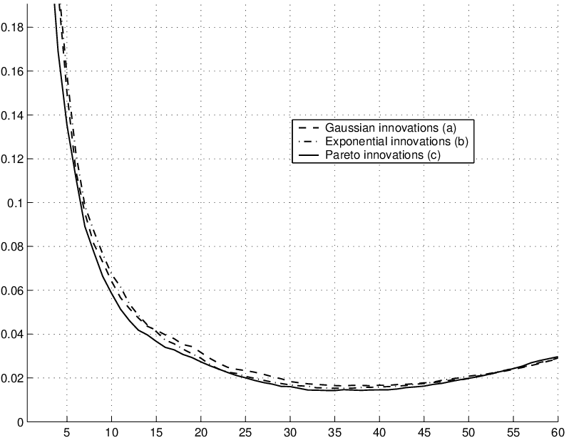
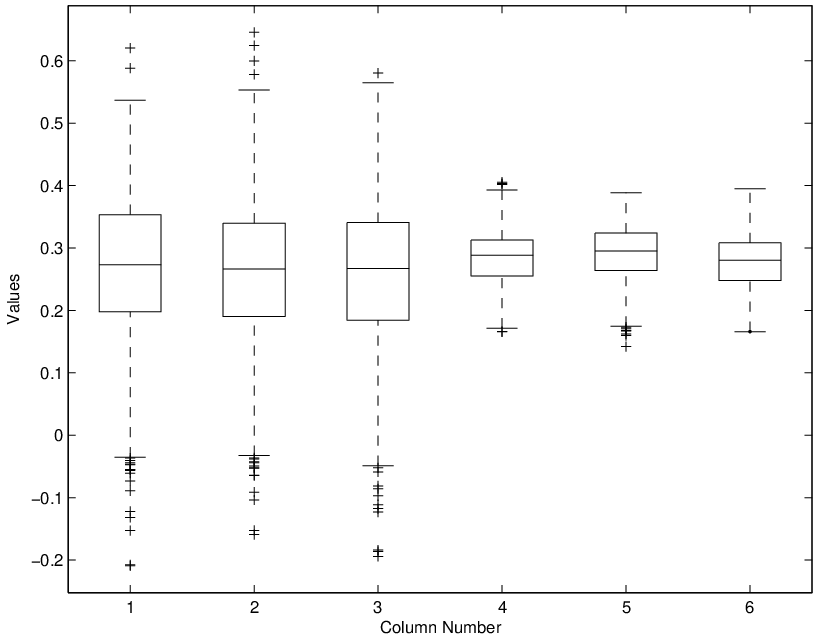
Whereas it is possible to simulate exactly a Gaussian FARIMA(p,d,q)(p,d,q) process (e.g. computing the covariance structure and using Levinson-Durbin algorithm), there is no general way to do it for non Gaussian processes. In the Monte-Carlo experiment, the process (Xt)(X_{t}) is obtained using a truncated MA(∞\infty) representation. For each realization of each process, we evaluate the squared error (d^m−d)(\hat{d}_{m}-d) and define the Monte Carlo MSE as the average of those errors. We have focused on the sensitivity with respect to the distribution of ZZ of the bandwidth mm which is optimal in the MSE sense. Figure 1 and Table 1 show that for sample size n=250n=250 the MSE is minimized at m=37m=37 or 3838 which means that the optimal bandwidth is about the same for those three linear processes. Figure 2 represents the box-and-whiskers plot of the GPH estimator for two different sample sizes and the three models we are concerned with. Here again, the sensitivity with respect to the distribution of the driving noise is hardly discernible. In Table 1 we displayed the value of the bias and of the mean square error of the GPH at this estimated optimal bandwidth.
Refer to caption
Figure 1. Comparisons of the MSE versus the bandwidth for the FARIMA processes (a),(b) and (c). Sample size n=250n=250
Refer to caption
Figure 2. Box-plot of the GPH estimator for processes (a),(b) and (c), sample size n=250,2500n=250,2500
(a) (b) (c)
nn=250 mo​p​tm_{opt} 37 37 38
𝔼MC​(d^mo​p​t−d){\mathbb{E}}_{\text{MC}}(\hat{d}_{m_{opt}}-d) -0.03037 -0.03751 -0.03871
𝔼MC​((d^mo​p​t−d)2){\mathbb{E}}_{\text{MC}}((\hat{d}_{m_{opt}}-d)^{2}) 0.01507 0.01508 0.01569
nn=500 mo​p​tm_{opt} 64 60 61
𝔼MC​(d^mo​p​t−d){\mathbb{E}}_{\text{MC}}(\hat{d}_{m_{opt}}-d) -0.02813 -0.01871 -0.02778
𝔼MC​((d^mo​p​t−d)2){\mathbb{E}}_{\text{MC}}((\hat{d}_{m_{opt}}-d)^{2}) 0.00807 0.00734 0.00766
nn=1000 mo​p​tm_{opt} 106 117 107
𝔼MC​(d^mo​p​t−d){\mathbb{E}}_{\text{MC}}(\hat{d}_{m_{opt}}-d) -0.01984 -0.02377 -0.01737
𝔼MC​((d^mo​p​t−d)2){\mathbb{E}}_{\text{MC}}((\hat{d}_{m_{opt}}-d)^{2}) 0.00507 0.00393 0.00438
nn=2500 mo​p​tm_{opt} 222 212 238
𝔼MC​(d^mo​p​t−d){\mathbb{E}}_{\text{MC}}(\hat{d}_{m_{opt}}-d) -0.01492 -0.00967 -0.02037
𝔼MC​((d^mo​p​t−d)2){\mathbb{E}}_{\text{MC}}((\hat{d}_{m_{opt}}-d)^{2}) 0.00207 0.00202 0.00219
nn=5000 mo​p​tm_{opt} 377 385 370
𝔼MC​(d^mo​p​t−d){\mathbb{E}}_{\text{MC}}(\hat{d}_{m_{opt}}-d) -0.01097 -0.00937 -0.01269
𝔼MC​((d^mo​p​t−d)2){\mathbb{E}}_{\text{MC}}((\hat{d}_{m_{opt}}-d)^{2}) 0.00106 0.00104 0.00097
Table 1. Optimal bandwidth, bias and MSE for processes (a), (b) and (c) and different sample sizes nn. All those values are estimated by Monte Carlo

Appendix A Edgeworth expansion for triangular arrays

In this section we recall the theorem established in Faÿ, Moulines, and Soulier (2004). Let (Zt)t∈ℤ(Z_{t})_{t\in{\mathbb{Z}}} be an i.i.d sequence and (𝐔n,j)j∈ℤ,n∈ℕ({\mathbf{U}}_{n,j})_{j\in{\mathbb{Z}},n\in{\mathbb{N}}} an array of vectors in ℝu{\mathbb{R}}^{u}, where uu is an integer. Define 𝐒n=∑j∈ℤ𝐔n,j​Zj{\mathbf{S}}_{n}=\sum_{j\in{\mathbb{Z}}}{\mathbf{U}}_{n,j}Z_{j} and let 𝐕n=∑j∈ℤ𝐔n,j​𝐔n,j′{\mathbf{V}}_{n}=\sum_{j\in{\mathbb{Z}}}{\mathbf{U}}_{n,j}{\mathbf{U}}^{\prime}_{n,j}. For 𝝂∈ℕu{\boldsymbol{\nu}}\in{\mathbb{N}}^{u}, 2≤|𝝂|≤s2\leq|{\boldsymbol{\nu}}|\leq s, denote χn,𝝂\chi_{n,{\boldsymbol{\nu}}} the cumulants of 𝐒n{\mathbf{S}}_{n}. Then χn,𝝂=κ|𝝂|​∑j∈ℤ𝐔n,j𝝂.\chi_{n,{\boldsymbol{\nu}}}=\kappa_{|{\boldsymbol{\nu}}|}\sum_{j\in{\mathbb{Z}}}{\mathbf{U}}_{n,j}^{{\boldsymbol{\nu}}}. where κr\kappa_{r} denotes the rr-th cumulant of Z1Z_{1}, r≤sr\leq s. Consider the following assumptions.

  • (B1)

    There exist positive constants v∗v_{*} and v∗v^{*} such that

    v∗≤lim infnvmin​[𝐕n]≤lim supnvmax​[𝐕n]≤v∗\displaystyle v_{*}\leq\liminf_{n}v_{\min}[{\mathbf{V}}_{n}]\leq\limsup_{n}v_{\max}[{\mathbf{V}}_{n}]\leq v^{*}

    where vmin​[𝐕n]v_{\min}[{\mathbf{V}}_{n}] (resp. vmax​[𝐕n]v_{\max}[{\mathbf{V}}_{n}]) is the smallest (resp. the largest) eigenvalue of 𝐕n{\mathbf{V}}_{n}.

  • (B2)

    There exist positive constants η\eta, c0c_{0}, a sequence (Mn)n∈ℕ(M_{n})_{n\in{\mathbb{N}}} of positive numbers, and a sequence (Jn)n∈ℕ(J_{n})_{n\in{\mathbb{N}}} of subsets of ℤ{\mathbb{Z}}, such that, for all n≥0n\geq 0

    supj∈ℤ‖𝐔n,j‖≤Mn\displaystyle\sup_{j\in{\mathbb{Z}}}\|{\mathbf{U}}_{n,j}\|\leq M_{n} (A.1)
    limn→∞Mn=0\displaystyle\lim_{n\to\infty}M_{n}=0 (A.2)
    card⁡(Jn)≤c0​Mn−2and∑j∈Jn‖𝐔n,j‖2∑j∈ℤ‖𝐔n,j‖2≥η.\displaystyle\mathrm{card}(J_{n})\leq c_{0}M_{n}^{-2}\quad\text{and}\quad\frac{\sum_{j\in J_{n}}\|{\mathbf{U}}_{n,j}\|^{2}}{\sum_{j\in{\mathbb{Z}}}\|{\mathbf{U}}_{n,j}\|^{2}}\geq\eta. (A.3)
  • (B3)

    There exist ζ≥1\zeta\geq 1 and a sequence (Mn)n∈ℕ(M_{n})_{n\in{\mathbb{N}}} satisfying (A.1) such that

    supn≥0Mnζ​∑j∈ℤ‖𝐔n,j‖<∞.\sup_{n\geq 0}M_{n}^{\zeta}\sum_{j\in{\mathbb{Z}}}\|{\mathbf{U}}_{n,j}\|<\infty\;.
Theorem 12 (Faÿ, Moulines, and Soulier, 2004).

Let s≥3s\geq 3, and p′≥0p^{\prime}\geq 0 be integers and p≥1p\geq 1 be a real number. Assume (A(A1))(s,p,p′s,p,p^{\prime}), (B(B1)) and (B(B2)). Assume in addition either (B(B3)) or p′≥sp^{\prime}\geq s in (A(A1))(s,p,p′s,p,p^{\prime}). Then, there exist a constant CC and an integer NN (depending only on the distribution of Z1Z_{1}, and the constants appearing in the assumptions) such that, for all n≥Nn\geq N, the distribution of 𝐒n{\mathbf{S}}_{n} has a density qnq_{n} with respect to Lebesgue measure on ℝu{\mathbb{R}}^{u} which satisfies

sup𝐱∈ℝu(1+‖𝐱‖s)​|qn​(𝐱)−∑r=0s−3Pr​(𝐱,𝐕n,{χn,𝝂})|≤C​∑j∈ℤ‖𝐔n,j‖s\displaystyle\sup_{{\mathbf{x}}\in{\mathbb{R}}^{u}}(1+\|{\mathbf{x}}\|^{s})\Bigl|q_{n}({\mathbf{x}})-\sum_{r=0}^{s-3}P_{r}({\mathbf{x}},{\mathbf{V}}_{n},\{\chi_{n,{\boldsymbol{\nu}}}\})\Bigr|\leq C\sum_{j\in{\mathbb{Z}}}\|{\mathbf{U}}_{n,j}\|^{s} (A.4)

Appendix B Proof of Theorem 1

The proof consists in checking that assumptions (B(B1)), (B(B2)) and (B(B3)) hold uniformly with respect to ψ∈𝒢⁡(α,β,δ)\psi\in\mathcal{G}(\alpha,\beta,\delta) and 𝐤{\mathbf{k}} for 𝐔n,j{\mathbf{U}}_{n,j}’s of the form (2.9). To prove (B(B1)), write 𝐕n​(𝐤)=𝐕⁡(𝐤)+𝐖n​(𝐤){\mathbf{V}}_{n}({\mathbf{k}})={\mathbf{V}}({\mathbf{k}})+{\mathbf{W}}_{n}({\mathbf{k}}), with 𝐕⁡(𝐤){\mathbf{V}}({\mathbf{k}}) defined in (3.5). Define ‖𝐖‖1=max⁡∑j=1v1≤i≤v⁡|wi,j|\|{\mathbf{W}}\|_{1}=\max_{1\leq i\leq v}\sum_{j=1}^{v}|w_{i,j}| for any matrix 𝐖=(wi,j)1≤i,j≤v{\mathbf{W}}=(w_{i,j})_{1\leq i,j\leq v}. Similarly to Hannan (1960, p. 54), we have under (3.1)

‖𝐖n​(𝐤)‖1≤C⁡(α,β)​n−1.\|{\mathbf{W}}_{n}({\mathbf{k}})\|_{1}\leq C(\alpha,\beta)n^{-1}. (B.1)

The matrices 𝐕⁡(𝐤){\mathbf{V}}({\mathbf{k}}) have the following algebraic property.

Lemma 13.

There exist two positive constants v∗v_{*} and v∗v^{*} such that

2​v∗≤infvmin​[𝐕⁡(𝐤)]≤supvmax​[𝐕⁡(𝐤)]≤2​v∗2v_{*}\leq\inf v_{\min}[{\mathbf{V}}({\mathbf{k}})]\leq\sup v_{\max}[{\mathbf{V}}({\mathbf{k}})]\leq 2v^{*} (B.2)

where the infimum and supremum are taken over all the uu-tuples of distinct integers in ℕu{\mathbb{N}}^{u}.

Proof.

Noting that trace​[𝐕​(𝐤)]=u\text{trace}[{\mathbf{V}}({\mathbf{k}})]=u,

vmax​[𝐕⁡(𝐤)]≤trace​[𝐕⁡(𝐤)]/2​u=1/2.\displaystyle v_{\max}[{\mathbf{V}}({\mathbf{k}})]\leq\text{trace}[{\mathbf{V}}({\mathbf{k}})]/{2u}=1/2. (B.3)

Take v∗=1/4v^{*}=1/4. Recall that k1<⋯<kuk_{1}<\dots<k_{u}. Note that, for any n≥2​ku+2​r+1n\geq 2k_{u}+2r+1, 𝐕⁡(𝐤){\mathbf{V}}({\mathbf{k}}) is the covariance matrix of

2​π​(cr,n,k1Y,sr,n,k1Y,…,cr,n,kuY,sr,n,kuY)\sqrt{2\pi}(c^{Y}_{r,n,k_{1}},s^{Y}_{r,n,k_{1}},\dotsc,c^{Y}_{r,n,k_{u}},s^{Y}_{r,n,k_{u}})

with cr,n,kY=(2πarn)−1/2∑t=1nht,nrYtcos(tλk)c^{Y}_{r,n,k}=(2\pi a_{r}n)^{-1/2}\sum_{t=1}^{n}h_{t,n}^{r}Y_{t}\cos(t\lambda_{k}) and sr,n,kY=(2πarn)−1/2∑t=1nht,nrYtsin(tλk)s^{Y}_{r,n,k}=(2\pi a_{r}n)^{-1/2}\sum_{t=1}^{n}h_{t,n}^{r}Y_{t}\sin(t\lambda_{k}) the sine and cosine transform of a unit-variance zero-mean Gaussian white noise (Yn)n∈ℤ(Y_{n})_{n\in{\mathbb{Z}}}. Recall that

cr,n,kY=ar−1/2∑l=0r(−1)l()lrc0,n,k+lYandsr,n,kY=ar−1/2∑l=0r(−1)l()lrs0,n,k+lY.c^{Y}_{r,n,k}=a_{r}^{-1/2}\sum_{l=0}^{r}(-1)^{l}\left({}^{r}_{l}\right)\;c^{Y}_{0,n,k+l}\ \ \ \text{and}\ \ \ s^{Y}_{r,n,k}=a_{r}^{-1/2}\sum_{l=0}^{r}(-1)^{l}\left({}^{r}_{l}\right)\;s^{Y}_{0,n,k+l}\;. (B.4)

The random variables c0,n,kc_{0,n,k} and s0,n,ks_{0,n,k}, k=1,…,[(n−1)/2]k=1,\dots,[(n-1)/2] are centered i.i.d Gaussian with variance 1/4​π1/4\pi. Assume that 𝐕⁡(𝐤){\mathbf{V}}({\mathbf{k}}) is not invertible. It yields that for some 2​u2u-tuple of reals (α1,β1,⋯,αu,βu)≠(0,0,⋯,0,0)(\alpha_{1},\beta_{1},\cdots,\alpha_{u},\beta_{u})\neq(0,0,\cdots,0,0),

∑j=1u(αj​cr,n,kj+βj​sr,n,kj)=𝕃20.\sum_{j=1}^{u}(\alpha_{j}c_{r,n,k_{j}}+\beta_{j}s_{r,n,k_{j}})\stackrel{{\scriptstyle\mathbb{L}^{2}}}{{=}}0.

Then by (B.4), there exists a linear combination of c0,n,kc_{0,n,k}’s and s0,n,ks_{0,n,k}’s that is equal to zero. c0,n,ku+rc_{0,n,k_{u}+r} and s0,n,ku+rs_{0,n,k_{u}+r} appear in this combination with coefficients ar−1/2(−1)rαua_{r}^{-1/2}(-1)^{r}\alpha_{u} and ar−1/2(−1)rβua_{r}^{-1/2}(-1)^{r}\beta_{u}, respectively. It follows from the independence and non-degeneracy of the c0,n,kc_{0,n,k}’s and s0,n,ks_{0,n,k}’s that αu=βu=0\alpha_{u}=\beta_{u}=0. Iterating the argument yields the contradiction αu=βu=αu−1=βu−1=⋯=α1=β1=0\alpha_{u}=\beta_{u}=\alpha_{u-1}=\beta_{u-1}=\cdots=\alpha_{1}=\beta_{1}=0. Thus for any uu-tuple 𝐤{\mathbf{k}} of distinct integers

vmin​[𝐕​(𝐤)]>0.\displaystyle v_{\min}[{\mathbf{V}}({\mathbf{k}})]>0. (B.5)

It remains to prove that vmin​[𝐕​(𝐤)]v_{\min}[{\mathbf{V}}({\mathbf{k}})] is bounded away from zero uniformly in 𝐤{\mathbf{k}}. Define

Ku={𝐤=(k1,⋯,ku′)∈ℕu′,1≤u′≤u,0<ki+1−ki≤r}.K_{u}=\{{\mathbf{k}}=(k_{1},\cdots,k_{u^{\prime}})\in{\mathbb{N}}^{u^{\prime}},1\leq u^{\prime}\leq u,0<k_{i+1}-k_{i}\leq r\}.

Note now that by (3.5), vmin​[𝐕​(𝐤)]v_{\min}[{\mathbf{V}}({\mathbf{k}})] is a function of the vector (k2−k1,k3−k2,⋯,ku−ku−1)(k_{2}-k_{1},k_{3}-k_{2},\cdots,k_{u}-k_{u-1}) thus taking finitely many different values on KuK_{u}. From the this remark and (B.5),

v1=definf𝐤∈Kuvmin​[𝐕⁡(𝐤)]>0v_{1}\stackrel{{\scriptstyle\mathrm{def}}}{{=}}\inf_{{\mathbf{k}}\in K_{u}}v_{\min}[{\mathbf{V}}({\mathbf{k}})]>0 (B.6)

since the infimum is taken on a finite set of positive values. Consider now a uu-tuple 𝐤{\mathbf{k}} that does not belong to KuK_{u}; In this case, for some i∈{1,⋯,u−1}i\in\{1,\cdots,u-1\}, ki+1−ki>rk_{i+1}-k_{i}>r, and then 𝐤{\mathbf{k}} may be partitioned as L≥2L\geq 2 blocks of indexes (𝐤1,…,𝐤L)({\mathbf{k}}_{1},\dots,{\mathbf{k}}_{L}) such that all the 𝐤i{\mathbf{k}}_{i}’s belong to KuK_{u} and, for all i∈{1,⋯,L−1}i\in\{1,\cdots,L-1\}, min⁡𝐤i+1−max⁡𝐤i>r\min{\mathbf{k}}_{i+1}-\max{\mathbf{k}}_{i}>r. Let lil_{i} denotes the length of the block 𝐤i,i=1,⋯,L{\mathbf{k}}_{i},i=1,\cdots,L. By this construction and (3.5), the matrix 𝐕⁡(𝐤){\mathbf{V}}({\mathbf{k}}) has a block-diagonal structure

𝐕⁡(𝐤)=(𝐕⁡(𝐤1)𝟎⋱𝟎𝐕⁡(𝐤L)).\displaystyle{\mathbf{V}}({\mathbf{k}})=\left(\begin{array}[]{ccc}{\mathbf{V}}({\mathbf{k}}_{1})&&\boldsymbol{0}\\ &\ddots&\\ \boldsymbol{0}&&{\mathbf{V}}({\mathbf{k}}_{L})\end{array}\right)\;.

Using (B.6),

vmin​[𝐕⁡(𝐤)]​(vmax​[𝐕⁡(𝐤)])2​u−1≥det[𝐕⁡(𝐤)]=∏i=1Ldet[𝐕⁡(𝐤i)]≥∏i=1Lv12​li=v12​u.v_{\min}[{\mathbf{V}}({\mathbf{k}})](v_{\max}[{\mathbf{V}}({\mathbf{k}})])^{2u-1}\geq\det[{\mathbf{V}}({\mathbf{k}})]=\prod_{i=1}^{L}\det[{\mathbf{V}}({\mathbf{k}}_{i})]\geq\prod_{i=1}^{L}v_{1}^{2l_{i}}=v_{1}^{2u}. (B.7)

We conclude from (B.7) and (B.3) that

vmin​[𝐕⁡(𝐤)]≥v12​u​22​u−1=:v2>0.v_{\min}[{\mathbf{V}}({\mathbf{k}})]\geq v_{1}^{2u}2^{2u-1}=:v_{2}>0. (B.8)

(B.2) follows from (B.6) and (B.8) with v∗=12​min⁡(v1,v2)v_{*}=\frac{1}{2}\min(v_{1},v_{2}). ∎

Proof of Theorem 1.

By (B.1) and Lemma 13, (B(B1)) holds with v∗v_{*} and v∗v^{*} of Lemma 13, for some N0N_{0}, n≥N0n\geq N_{0} and uniformly in 𝐤,α{\mathbf{k}},\alpha and β\beta. With (B.3),

|∑j∈ℤ∥𝐔n,j(𝐤)∥2−u|=|trace[𝐕n(𝐤)]−u|≤C(α,β)n−1/2.\displaystyle\Bigl|\sum_{j\in{\mathbb{Z}}}\|{\mathbf{U}}_{n,j}({\mathbf{k}})\|^{2}-u\Bigr|=\left|\text{trace}[{\mathbf{V}}_{n}({\mathbf{k}})]-u\right|\leq C(\alpha,\beta)n^{-1/2}. (B.9)

Prove now that (B(B2)) is verified. Since ff is bounded away from zero and ∑j∈ℤ|ψj|≤β<∞\sum\nolimits_{j\in{\mathbb{Z}}}|\psi_{j}|\leq\beta<\infty, (A.1) and (A.2) are verified with Mn=defC(r)βα−1/2n−1/2M_{n}\stackrel{{\scriptstyle\mathrm{def}}}{{=}}C(r)\beta\alpha^{-1/2}n^{-1/2}. Put Jn={j,|j|<2​n}J_{n}=\{j,|j|<2n\}. Then card​(Jn)≤c0​Mn−2\text{card}(J_{n})\leq c_{0}M_{n}^{-2} for some c0c_{0} depending only on r,α,βr,\alpha,\beta and

∑|j|∈ℤ∖Jn‖𝐔n,j​(𝐤)‖2≤C⁡(r)​α−2​n−1​∑|j|≥2​n(∑t=1n|ψt+j|)2≤C⁡(r)​α−2​∑|j|≥2​n∑t=1nψt+j2≤C⁡(r)​α−2​∑|j|≥n|j|​ψj2.\sum_{|j|\in{\mathbb{Z}}\setminus J_{n}}\|{\mathbf{U}}_{n,j}({\mathbf{k}})\|^{2}\leq C(r)\alpha^{-2}n^{-1}\sum_{|j|\geq 2n}\left(\sum_{t=1}^{n}|\psi_{t+j}|\right)^{2}\\ \leq C(r)\alpha^{-2}\sum_{|j|\geq 2n}\sum_{t=1}^{n}\psi_{t+j}^{2}\leq C(r)\alpha^{-2}\sum_{|j|\geq n}|j|\psi_{j}^{2}. (B.10)

Under (3.1), |ψj|≤β|j|−1/2−δ|\psi_{j}|\leq\beta|j|^{-1/2-\delta} so that

∑|j|≥n|j|​ψj2≤β​n−2​δ​∑|j|≥n|j|1/2+δ​|ψj|≤β2​n−2​δ\displaystyle\sum_{|j|\geq n}|j|\psi_{j}^{2}\leq\beta n^{-2\delta}\sum_{|j|\geq n}|j|^{1/2+\delta}|\psi_{j}|\leq\beta^{2}n^{-2\delta} (B.11)

For any ϵ>0\epsilon>0 and large enough nn, ∑|j|≥n‖𝐔n,j​(𝐤)‖2≤ϵ\sum_{|j|\geq n}\|{\mathbf{U}}_{n,j}({\mathbf{k}})\|^{2}\leq\epsilon uniformly in 𝐤{\mathbf{k}} and ψ∈𝒢⁡(α,β,δ)\psi\in\mathcal{G}(\alpha,\beta,\delta). (A.3) follows from (B.9), (B.10) and (B.11). Finally,

∑j∈ℤ∥𝐔n,j(𝐤)∥≤C(r)α−1/2n−1/2∑t=1n∑j∈ℤ|ψt+j|=C(r)α−1/2n1/2∑j∈ℤ|ψj|≤C(r)α−1/2βn1/2=C(r)2α−1β2Mn−1\sum_{j\in{\mathbb{Z}}}\|{\mathbf{U}}_{n,j}({\mathbf{k}})\|\leq C(r)\alpha^{-1/2}n^{-1/2}\sum_{t=1}^{n}\sum_{j\in{\mathbb{Z}}}|\psi_{t+j}|=C(r)\alpha^{-1/2}n^{1/2}\sum_{j\in{\mathbb{Z}}}|\psi_{j}|\\ \leq C(r)\alpha^{-1/2}\beta n^{1/2}=C(r)^{2}\alpha^{-1}\beta^{2}M_{n}^{-1}

so that (B(B3)) holds with ζ=1\zeta=1. ∎

Appendix C Proof of Lemma 8

The proof is an adaptation of Lang and Soulier (2002) to fit our need of uniformity of the bounds with respect to the function ψ\psi whether it belongs to ℱglobal\mathcal{F}_{\mathrm{global}} or ℱlocal\mathcal{F}_{\mathrm{local}} only. For sake of brevity, the proof is omitted and we refer the interested reader to their paper. It derives from their more general analytical lemma that we recall here.

Lemma 14 (Lang and Soulier (2002)).

Let q∈ℕq\in{\mathbb{N}}, K≥1K\geq 1, ϑ∈(0,π]\vartheta\in(0,\pi]. Let ψ\psi be an integrable function on [−π,π][-\pi,\pi], such that for all x∈(0,ϑ]∖{0}x\in(0,\vartheta]\setminus\{0\}, ψ​(−x)=ψ¯​(x)\psi(-x)=\bar{\psi}(x) and

|ψ⁡(x)−ψ⁡(y)|≤K​|ψ⁡(x)|+|ψ⁡(y)|x∧y​|x−y|,for all​(x,y)∈(0,ϑ]×(0,ϑ]\displaystyle|\psi(x)-\psi(y)|\leq K\frac{|\psi(x)|+|\psi(y)|}{x\wedge y}\,|x-y|,\quad\text{for all}(x,y)\in(0,\vartheta]\times(0,\vartheta] (C.1)

Assume that |ψ||\psi| is regularly varying at zero with index ρ\rho and that

ψ⁡(x)=xρ​c​(x)​exp⁡{∫xϑg⁡(s)s​𝑑s}\psi(x)=x^{\rho}c(x)\exp\left\{\int_{x}^{\vartheta}\frac{g(s)}{s}\,{\mathrm{d}}s\right\}

with (i) limx→0g⁡(x)=0\lim_{x\to 0}g(x)=0; (ii) limx→0c⁡(x)\lim_{x\to 0}c(x) exists in (0,∞)(0,\infty). Let DnD_{n} be such that for x∈[−π,π]x\in[-\pi,\pi],

|Dn​(x)|≤C​n1/2(1+n​|x|)q+1.\displaystyle|D_{n}(x)|\leq C\frac{n^{1/2}}{(1+n|x|)^{q+1}}. (C.2)
  • •

    If ρ∈(−1,2​q+1)\rho\in(-1,2q+1), there exists a constant CC such that, for all n≥1n\geq 1 and all kk such that 0<xk≤ϑ/20<x_{k}\leq\vartheta/2,

    |∫−ππ(ψ⁡(x)ψ⁡(xk)−1)​|Dn​(xk−x)|2​𝑑x|≤C​logν⁡(q)⁡(k)​k−1.\displaystyle\left|\int_{-\pi}^{\pi}\left(\frac{\psi(x)}{\psi(x_{k})}-1\right)|D_{n}(x_{k}-x)|^{2}\,{\mathrm{d}}x\right|\leq C\log^{\nu(q)}(k)k^{-1}. (C.3)

    with ν⁡(0)=1\nu(0)=1 and ν⁡(q)=0\nu(q)=0 if q≥1q\geq 1.

  • •

    If ρ∈(−1/2,q+1/2)\rho\in(-1/2,q+1/2), there exists a constant CC such that, for all n≥1n\geq 1 and all integers k,jk,j such that 0<xk≠xj≤ϑ/20<x_{k}\neq x_{j}\leq\vartheta/2,

    |∫−ππ(ψ⁡(x)ψ⁡(xk)−1)​Dn​(xk−x)​Dn​(xj−x)¯​dx|+|∫−ππ(ψ⁡(x)ψ⁡(xk)−1)​Dn​(xk−x)​Dn​(x+xj)​dx|≤{C(1+|ψ(xj)/ψ(k)|)|k−j|−q(j∨k)−1≤C(jk)−1/2(q>0);C(jk)−1/2log(j∨k)(q=0).\left|\int_{-\pi}^{\pi}\left(\frac{\psi(x)}{\psi(x_{k})}-1\right)D_{n}(x_{k}-x)\overline{D_{n}(x_{j}-x)}\,{\mathrm{d}}x\right|\\ +\left|\int_{-\pi}^{\pi}\left(\frac{\psi(x)}{\psi(x_{k})}-1\right)D_{n}(x_{k}-x)D_{n}(x+x_{j})\,{\mathrm{d}}x\right|\\ \leq\left\{\begin{array}[]{ll}C(1+|\psi(x_{j})/\psi(_{k})|)|k-j|^{-q}(j\vee k)^{-1}\leq C(jk)^{-1/2}&(q>0);\\ C(jk)^{-1/2}\log(j\vee k)&(q=0).\end{array}\right. (C.4)
  • •

    For any β>0\beta>0, if ρ∈(−1,2​q+1)\rho\in(-1,2q+1), for any integer kk such that 0<xk≤ϑ/20<x_{k}\leq\vartheta/2,

    |∫−ππψ⁡(x)​|x|βψ⁡(xk)​|Dn​(xk−x)|2​𝑑x|≤C⁡{k−2​q−1+(k/n)β}.\displaystyle\left|\int_{-\pi}^{\pi}\frac{\psi(x)|x|^{\beta}}{\psi(x_{k})}|D_{n}(x_{k}-x)|^{2}\,{\mathrm{d}}x\right|\leq C\left\{k^{-2q-1}+(k/n)^{\beta}\right\}. (C.5)
  • •

    If ρ∈(−1/2,q+1/2)\rho\in(-1/2,q+1/2), for any integers j,kj,k such that 0<xk≠xj≤ϑ/20<x_{k}\neq x_{j}\leq\vartheta/2,

    |∫−ππψ⁡(x)​|x|βψ⁡(xk)​|Dn​(xk−x)​Dn​(xj−x)¯|​dx|+|∫−ππψ⁡(x)​|x|βψ⁡(xk)​|Dn​(xk−x)​Dn​(xj+x)|​dx|≤C⁡(1+|ψ⁡(xj)/ψ⁡(xk)|)​{(j​k)−q​(j∨k)−1+|j−k|−q−1​((j∨k)/n)β​logν⁡(q)⁡(j∨k)}≤C{(jk)−1/2+((j∨k)/n)βlogν⁡(q)(j∨k)}.\left|\int_{-\pi}^{\pi}\frac{\psi(x)|x|^{\beta}}{\psi(x_{k})}|D_{n}(x_{k}-x)\overline{D_{n}(x_{j}-x)}|\,{\mathrm{d}}x\right|+\left|\int_{-\pi}^{\pi}\frac{\psi(x)|x|^{\beta}}{\psi(x_{k})}|D_{n}(x_{k}-x)D_{n}(x_{j}+x)|\,{\mathrm{d}}x\right|\\ \leq C(1+|\psi(x_{j})/\psi(x_{k})|)\left\{(jk)^{-q}(j\vee k)^{-1}+|j-k|^{-q-1}((j\vee k)/n)^{\beta}\log^{\nu(q)}(j\vee k)\right\}\\ \leq C\left\{(jk)^{-1/2}+((j\vee k)/n)^{\beta}\log^{\nu(q)}(j\vee k)\right\}. (C.6)

Appendix D Proof of Theorem 6

The proof of Theorem 6 consists in checking that assumptions (B(B1)), (B(B2)) hold uniformly.

Lemma 15.

There exist integers N0N_{0}, K0K_{0}, and v∗>0,v∗>0v_{*}>0,v^{*}>0 (depending only on ϑ,β,δ,Δ,μ\vartheta,\beta,\delta,\Delta,\mu) such that, for all n≥N0n\geq N_{0}, we have,

  1. (1)

    for all uu-tuple 𝐤{\mathbf{k}} of distinct integers, 1≤min⁡𝐤≤max⁡𝐤≤mn1\leq\min{\mathbf{k}}\leq\max{\mathbf{k}}\leq m_{n},

    vmax​[𝐕n​(𝐤)]≤v∗;v_{\max}[{\mathbf{V}}_{n}({\mathbf{k}})]\leq v^{*}\;; (D.1)
  2. (2)

    for all integer kk, 1≤k≤mn1\leq k\leq m_{n}

    v∗≤vmin​[𝐕n​(k)];v_{*}\leq v_{\min}[{\mathbf{V}}_{n}(k)]\;; (D.2)
  3. (3)

    for all uu-tuple 𝐤{\mathbf{k}} of distinct integers, K0≤min⁡𝐤≤max⁡𝐤≤mnK_{0}\leq\min{\mathbf{k}}\leq\max{\mathbf{k}}\leq m_{n},

    v∗≤vmin​[𝐕n​(𝐤)].v_{*}\leq v_{\min}[{\mathbf{V}}_{n}({\mathbf{k}})]\;. (D.3)
Proof.

As in Appendix B, we put 𝐕n​(𝐤)=𝐕⁡(𝐤)+𝐖n​(𝐤){\mathbf{V}}_{n}({\mathbf{k}})={\mathbf{V}}({\mathbf{k}})+{\mathbf{W}}_{n}({\mathbf{k}}) where 𝐕⁡(𝐤){\mathbf{V}}({\mathbf{k}}) is defined in (3.5). Applying Lemma 8, we obtain

‖𝐖n​(𝐤)‖1≤C⁡(ϑ,β,δ,Δ,μ)​{1k1+(mnn)β​log⁡(mnn)under(4.5),1k1under(4.6).\|{\mathbf{W}}_{n}({\mathbf{k}})\|_{1}\leq C(\vartheta,\beta,\delta,\Delta,\mu)\begin{cases}\frac{1}{k_{1}}+\left(\frac{m_{n}}{n}\right)^{\beta}\log\left(\frac{m_{n}}{n}\right)&\text{under}\quad(\ref{cond:local}),\\ \frac{1}{k_{1}}&\text{under}\quad(\ref{cond:global}).\end{cases} (D.4)

(D.1) follows immediately. The proof of (D.3) follows by picking N0,K0N_{0},K_{0} large enough. For (D.2), it remains to prove that for any integer kk, 1≤k≤K01\leq k\leq K_{0}, 𝐕n​(k){\mathbf{V}}_{n}(k) converges to a positive definite matrix 𝐕~​(k)\widetilde{\mathbf{V}}(k) and that this convergence is uniform w.r.t to ψ\psi, for ψ∈ℱlocal​(ϑ,β,δ,Δ,μ)\psi\in\mathcal{F}_{\mathrm{local}}(\vartheta,\beta,\delta,\Delta,\mu) or ψ∈ℱglobal​(ϑ,β,δ,Δ,μ)\psi\in\mathcal{F}_{\mathrm{global}}(\vartheta,\beta,\delta,\Delta,\mu). What follows is an adaptation of (Iouditsky et al., 2001, Lemma 7.3). Write

𝔼[|ωr,n,k|2]=1f⁡(λk)(∫|λ|≤ϑ​π+∫|λ|>ϑ​π)|Dr,n(λ−λk)|2f(λ)dλ=:A1+A2{\mathbb{E}}[|\omega_{r,n,k}|^{2}]=\frac{1}{f(\lambda_{k})}\left(\int_{|\lambda|\leq\vartheta\pi}+\int_{|\lambda|>\vartheta\pi}\right)|D_{r,n}(\lambda-\lambda_{k})|^{2}f(\lambda)d\lambda=:A_{1}+A_{2} (D.5)

where Dr,nD_{r,n} is defined in (2.2). For n≥4​π​K0/ϑn\geq 4\pi K_{0}/\vartheta, 1≤k≤K01\leq k\leq K_{0} and |λ|≥ϑ​π|\lambda|\geq\vartheta\pi, |n⁡(λ−λk)|≥n​ϑ/2|n(\lambda-\lambda_{k})|\geq n\vartheta/2. Using (2.3) and (4.1), we get

A2≤C​λk2​dλk2​d​f​(λk)​n−2​r−1​∫|λ|>ϑ​πλ2​d​f​(λ)​𝑑λ≤C​n−2​rA_{2}\leq\frac{C\lambda_{k}^{2d}}{\lambda_{k}^{2d}f(\lambda_{k})}n^{-2r-1}\int_{|\lambda|>\vartheta\pi}\lambda^{2d}f(\lambda)d\lambda\leq Cn^{-2r} (D.6)

By change of variable,

A1=n2​d​|1−e−i​λk|2​df∗​(λk)∫|λ|≤n​ϑ|n−1/2Dr,n(λ/n−λk)|2n−2​d|1−e−iλ/n|−2​df∗(λn)dλ.A_{1}=\frac{n^{2d}|1-{\mathrm{e}}^{-{\mathrm{i}}\lambda_{k}}|^{2d}}{f^{*}(\lambda_{k})}\int_{|\lambda|\leq n\vartheta}\left|n^{-1/2}D_{r,n}(\lambda/n-\lambda_{k})\right|^{2}n^{-2d}|1-{\mathrm{e}}^{-{\mathrm{i}}\lambda/n}|^{-2d}f^{*}(\frac{\lambda}{n})d\lambda.

Write limn→∞n−1/2Dr,n(λ/n)=12​π​ar∫01(1−e2​i​π​s)re−i​s​λds=:h^r(λ)\lim_{n\to\infty}n^{-1/2}D_{r,n}(\lambda/n)=\frac{1}{\sqrt{2\pi a_{r}}}\int_{0}^{1}(1-{\mathrm{e}}^{2{\mathrm{i}}\pi s})^{r}{\mathrm{e}}^{-{\mathrm{i}}s\lambda}ds=:\hat{h}_{r}(\lambda). By Riemann approximation, it can be seen that |n−1/2Dr,n(λ/n)−h^r(λ)|≤C(1+|λ|)/n|n^{-1/2}D_{r,n}(\lambda/n)-\hat{h}_{r}(\lambda)|\leq C(1+|\lambda|)/n. Note also that |h^r​(λ)|≤C​|λ|−r−1|\hat{h}_{r}(\lambda)|\leq C|\lambda|^{-r-1}. Then

|A1−n2​d​|1−ei​λk|2​df∗​(λk)×∫−n​ϑn​ϑ|h^r​(λ−2​π​k)|2​n−2​d​|1−ei​λ/n|−2​d​f∗​(λn)​𝑑λ|≤C​k2​d​n−r≤C​n−r.\Biggl|A_{1}-\frac{n^{2d}|1-{\mathrm{e}}^{{\mathrm{i}}\lambda_{k}}|^{2d}}{f^{*}(\lambda_{k})}\times\int_{-n\vartheta}^{n\vartheta}\left|\hat{h}_{r}(\lambda-2\pi k)\right|^{2}n^{-2d}|1-{\mathrm{e}}^{{\mathrm{i}}\lambda/n}|^{-2d}f^{*}(\frac{\lambda}{n})d\lambda\Biggr|\\ \leq Ck^{2d}n^{-r}\leq Cn^{-r}. (D.7)

Here and in the following, CC is a generic constant which depends only on ϑ,β,δ,Δ,μ,r\vartheta,\beta,\delta,\Delta,\mu,r and K0K_{0}. For |λ|≤n​ϑ|\lambda|\leq n\vartheta, using (4.5),

f∗​(0)f∗​(λk)​|n−2​d​|1−ei​λ/n|−2​d−|λ|−2​d|+|f∗​(λn)−f∗​(0)|f∗​(λk)​n−2​d​|1−ei​λ/n|−2​d\displaystyle\frac{f^{*}(0)}{f^{*}(\lambda_{k})}\left|n^{-2d}|1-{\mathrm{e}}^{{\mathrm{i}}\lambda/n}|^{-2d}-|\lambda|^{-2d}\right|+\frac{|f^{*}(\frac{\lambda}{n})-f^{*}(0)|}{f^{*}(\lambda_{k})}n^{-2d}|1-{\mathrm{e}}^{{\mathrm{i}}\lambda/n}|^{-2d}
≤C⁡{|n−2​d​|1−ei​λ/n|−2​d−|λ|−2​d|+n−2​d​|1−ei​λ/n|−2​d​|λn|β′}\displaystyle\leq C\left\{\left|n^{-2d}|1-{\mathrm{e}}^{{\mathrm{i}}\lambda/n}|^{-2d}-|\lambda|^{-2d}\right|+n^{-2d}|1-{\mathrm{e}}^{{\mathrm{i}}\lambda/n}|^{-2d}|\frac{\lambda}{n}|^{\beta^{\prime}}\right\} (D.8)

with β′=β∧1\beta^{\prime}=\beta\wedge 1. For x∈[−π,π],2π​|x|≤|ei​x−1|=|2​sin⁡x2|≤|x|x\in[-\pi,\pi],\frac{2}{\pi}|x|\leq|{\mathrm{e}}^{{\mathrm{i}}x}-1|=|2\sin\frac{x}{2}|\leq|x| and ||ei​x−1|−|x||≤x2/2||{\mathrm{e}}^{{\mathrm{i}}x}-1|-|x||\leq\ x^{2}/2. Also, for any υ∈ℝ,x>0,y>0,|xυ−yυ|≤|υ​|(xυ−1∨yυ−1)|​x−y|\upsilon\in{\mathbb{R}},x>0,y>0,|x^{\upsilon}-y^{\upsilon}|\leq|\upsilon|(x^{\upsilon-1}\vee y^{\upsilon-1})|x-y|. Using those relations, write, for λ∈[−n​π,n​π]\lambda\in[-n\pi,n\pi],

|n−2​d​|1−ei​λ/n|−2​d−|λ|−2​d|\displaystyle\Bigl|n^{-2d}|1-{\mathrm{e}}^{{\mathrm{i}}\lambda/n}|^{-2d}-|\lambda|^{-2d}\Bigr| ≤C​n−2​d​|λn|−2​d−1​||1−ei​λ/n|−|λn||\displaystyle\leq Cn^{-2d}|\frac{\lambda}{n}|^{-2d-1}\Bigl||1-{\mathrm{e}}^{{\mathrm{i}}\lambda/n}|-|\frac{\lambda}{n}|\Bigr|
≤C​n−1​|λ|−2​d+1\displaystyle\leq Cn^{-1}|\lambda|^{-2d+1}

Then

∫−n​ϑn​ϑ\displaystyle\int_{-n\vartheta}^{n\vartheta} |h^r​(2​π​k−λ)|2​|n−2​d​|1−ei​λ/n|−2​d−|λ|−2​d|​d​λ\displaystyle|\hat{h}_{r}(2\pi k-\lambda)|^{2}\left|n^{-2d}|1-{\mathrm{e}}^{{\mathrm{i}}\lambda/n}|^{-2d}-|\lambda|^{-2d}\right|d\lambda
≤C​n−1​∫−n​ϑn​ϑ|h^r​(2​π​k−λ)|2​|λ|−2​d+1​𝑑λ\displaystyle\leq Cn^{-1}\int_{-n\vartheta}^{n\vartheta}|\hat{h}_{r}(2\pi k-\lambda)|^{2}|\lambda|^{-2d+1}d\lambda
≤C​n−1​∫−n​ϑn​ϑ|h^r​(2​π​k−λ)|2​|λ|2​r​𝑑λ≤C​n−1\displaystyle\leq Cn^{-1}\int_{-n\vartheta}^{n\vartheta}|\hat{h}_{r}(2\pi k-\lambda)|^{2}|\lambda|^{2r}d\lambda\leq Cn^{-1} (D.9)

and

∫−n​ϑn​ϑ\displaystyle\int_{-n\vartheta}^{n\vartheta} |h^r​(2​π​k−λ)|2​n−2​d​|1−ei​λ/n|−2​d​|λn|β′​d​λ\displaystyle|\hat{h}_{r}(2\pi k-\lambda)|^{2}n^{-2d}|1-{\mathrm{e}}^{{\mathrm{i}}\lambda/n}|^{-2d}|\frac{\lambda}{n}|^{\beta^{\prime}}d\lambda
≤n−β′​∫−n​ϑn​ϑ|h^r​(2​π​k−λ)|2​|λ|−2​d+β′​𝑑λ\displaystyle\leq\ n^{-\beta^{\prime}}\int_{-n\vartheta}^{n\vartheta}|\hat{h}_{r}(2\pi k-\lambda)|^{2}|\lambda|^{-2d+\beta^{\prime}}d\lambda
≤C​n−β′.\displaystyle\leq Cn^{-\beta^{\prime}}. (D.10)

Gathering (D.5), (D.6), (D.7), (D.8), (D.9), (D.10) yields

|𝔼⁡[|ωr,n,k|2]−(2​π)2​d​k2​d​f∗​(0)f∗​(λk)​∫∞+∞|h^r​(λ−2​π​k)|2​|λ|−2​d​𝑑λ|≤C​n−β′\Biggl|{\mathbb{E}}[|\omega_{r,n,k}|^{2}]-\frac{(2\pi)^{2d}k^{2d}f^{*}(0)}{f^{*}(\lambda_{k})}\int_{\infty}^{+\infty}\left|\hat{h}_{r}(\lambda-2\pi k)\right|^{2}|\lambda|^{-2d}d\lambda\Biggr|\leq Cn^{-\beta^{\prime}}

Similar arguments leads to

|𝔼⁡[ωr,n,k2]−(2​π)2​d​k2​d​f∗​(0)f∗​(λk)​∫∞+∞h^r​(λ−2​π​k)​h^r​(λ+2​π​k)​|λ|−2​d​𝑑λ|≤C​n−β′\Biggl|{\mathbb{E}}[\omega_{r,n,k}^{2}]-\frac{(2\pi)^{2d}k^{2d}f^{*}(0)}{f^{*}(\lambda_{k})}\int_{\infty}^{+\infty}\hat{h}_{r}(\lambda-2\pi k)\hat{h}_{r}(\lambda+2\pi k)|\lambda|^{-2d}d\lambda\Biggr|\leq Cn^{-\beta^{\prime}}

Defining the scalar product (u,v)d=∫ℝu⁡(λ)​v​(λ)​|λ|−2​d​𝑑λ(u,v)_{d}=\int_{\mathbb{R}}u(\lambda)v(\lambda)|\lambda|^{-2d}d\lambda, Then det𝐕n​(k)\det{\mathbf{V}}_{n}(k) is uniformly approximated by the Gram determinant of the functions h^r​(λ−2​k​π)\hat{h}_{r}(\lambda-2k\pi) and h^r​(λ+2​k​π)\hat{h}_{r}(\lambda+2k\pi) associated with the product (⋅,⋅)d(\cdot,\cdot)_{d} and then is a continuous function of ηk​(d):=limn→∞𝔼⁡[|ωr,n,k|2]\eta_{k}(d):=\lim_{n\rightarrow\infty}{\mathbb{E}}[\left|\omega_{r,n,k}\right|^{2}] and ηk′​(d):=limn→∞𝔼⁡[ωr,n,k2]\eta^{\prime}_{k}(d):=\lim_{n\rightarrow\infty}{\mathbb{E}}[\omega_{r,n,k}^{2}].. The whole set of functions h^r​(λ+2​j​π),j∈ℤ\hat{h}_{r}(\lambda+2j\pi),j\in{\mathbb{Z}} is linearly independent, so that those determinant are positive. Using continuity of ηk\eta_{k} and ηk′\eta^{\prime}_{k} w.r.t. dd, the infimum on the compact set [−Δ,δ][-\Delta,\delta] and the minimum over k=1,…,K0k=1,\dots,K_{0} is positive too, which concludes the proof. ∎

Lemma 16.

There exists a constant CC (depending only on ϑ\vartheta, β\beta, δ\delta, Δ\Delta, μ\mu,rr) such that for all k∈{1,…,n~}k\in\{1,\dots,\tilde{n}\},

1n​f​(λk)|∑t=1nht,nrψt+jei​t​λk|≤Cn−1/2.\frac{1}{\sqrt{nf(\lambda_{k})}}\left|\sum_{t=1}^{n}h_{t,n}^{r}\psi_{t+j}{\mathrm{e}}^{{\mathrm{i}}t\lambda_{k}}\right|\leq Cn^{-1/2}. (D.11)
Proof.

The main tool of the proof is the bound (2.3) and the technique are the same as the one used in the proof of Lemma 8. Decompose

|ψ⁡(λk)|−1​12​π​ar​n​∑t=1nht,nr​ψt−j​ei​t​λk=|ψ⁡(λk)|∫−ππ−1⁡ψ⁡(λ)​ei​j​λ​Dn,r​(λk−λ)​𝑑λ\displaystyle|\psi(\lambda_{k})|^{-1}\frac{1}{\sqrt{2\pi a_{r}n}}\sum_{t=1}^{n}h_{t,n}^{r}\psi_{t-j}{\mathrm{e}}^{{\mathrm{i}}t\lambda_{k}}=|\psi(\lambda_{k})|^{-1}\int_{-\pi}^{\pi}\psi(\lambda){\mathrm{e}}^{{\mathrm{i}}j\lambda}D_{n,r}(\lambda_{k}-\lambda)d\lambda

into

A1\displaystyle A_{1} =|ψ(λk)|−1(∫−π−ϑ+∫ϑπ)ψ(λ)ei​j​λDn,r(λk−λ)dλ,\displaystyle=|\psi(\lambda_{k})|^{-1}\left(\int_{-\pi}^{-\vartheta}+\int_{\vartheta}^{\pi}\right)\psi(\lambda){\mathrm{e}}^{{\mathrm{i}}j\lambda}D_{n,r}(\lambda_{k}-\lambda)d\lambda,
A2\displaystyle A_{2} =|ψ⁡(λk)|−1​ψ∗​(0)​∫−ϑϑ(1−ei​λ)−d​ei​j​λ​Dn,r​(λk−λ)​𝑑λ,\displaystyle=|\psi(\lambda_{k})|^{-1}\psi^{*}(0)\int_{-\vartheta}^{\vartheta}(1-{\mathrm{e}}^{{\mathrm{i}}\lambda})^{-d}{\mathrm{e}}^{{\mathrm{i}}j\lambda}D_{n,r}(\lambda_{k}-\lambda)d\lambda,
A3\displaystyle A_{3} =|ψ⁡(λk)|∫−ϑϑ−1⁡(1−ei​λ)−d​(ψ∗​(λ)−ψ∗​(0))​ei​j​λ​Dn,r​(λk−λ)​𝑑λ.\displaystyle=|\psi(\lambda_{k})|^{-1}\int_{-\vartheta}^{\vartheta}(1-{\mathrm{e}}^{{\mathrm{i}}\lambda})^{-d}(\psi^{*}(\lambda)-\psi^{*}(0)){\mathrm{e}}^{{\mathrm{i}}j\lambda}D_{n,r}(\lambda_{k}-\lambda)d\lambda.

By Eq. (2.3), if |λ|∈[ϑ,π]|\lambda|\in[\vartheta,\pi], |Dn,r(λk−λ)|≤Cn−1/2−r|D_{n,r}(\lambda_{k}-\lambda)|\leq Cn^{-1/2-r}. Note that n−1​λkd=n−1​λk−1​λkd+1≤1/(2​π​k)n^{-1}\lambda_{k}^{d}=n^{-1}\lambda_{k}^{-1}\lambda_{k}^{d+1}\leq 1/(2\pi k). (4.1) implies that |A1|≤Cn1/2−rk−1≤Cn−1/2|A_{1}|\leq Cn^{1/2-r}k^{-1}\leq Cn^{-1/2}. Consider A2A_{2}. Since ∫−ππDn,r​(λ)​𝑑λ=0\int_{-\pi}^{\pi}D_{n,r}(\lambda)d\lambda=0,

A2=∫−ϑϑΔ⁡(λ,λk)​Dn,r​(λk−λ)​𝑑λ,Δ⁡(λ,λk)=((1−ei​λ)−d−(1−ei​λk)−d)​ei​j​λ​|ψ⁡(λk)|−1.A_{2}=\int_{-\vartheta}^{\vartheta}\Delta(\lambda,\lambda_{k})D_{n,r}(\lambda_{k}-\lambda)d\lambda,\quad\Delta(\lambda,\lambda_{k})=\left((1-{\mathrm{e}}^{{\mathrm{i}}\lambda})^{-d}-(1-{\mathrm{e}}^{{\mathrm{i}}\lambda_{k}})^{-d}\right){\mathrm{e}}^{{\mathrm{i}}j\lambda}|\psi(\lambda_{k})|^{-1}.

Decompose this integral on the intervals [−ϑ,−λk/2][-\vartheta,-\lambda_{k}/2], [−λk/2,λk/2][-\lambda_{k}/2,\lambda_{k}/2], [λk/2,2​λk][\lambda_{k}/2,2\lambda_{k}] and [2​λk,ϑ][2\lambda_{k},\vartheta]. If λ∈[−λk/2,λk/2]\lambda\in[-\lambda_{k}/2,\lambda_{k}/2], then |Dn,r​(λk−λ)|≤C​n​k−r−1|D_{n,r}(\lambda_{k}-\lambda)|\leq C\sqrt{n}k^{-r-1} and |Δ⁡(λ,λk)|≤C⁡(|λ|−d​λkd+1)|\Delta(\lambda,\lambda_{k})|\leq C\left(|\lambda|^{-d}\lambda_{k}^{d}+1\right). Hence :

|∫−λk/2λk/2Δ(λ,λk)Dn,r(λk−λ)dλ|≤Ck−rn−1/2.\left|\int_{-\lambda_{k}/2}^{\lambda_{k}/2}\Delta(\lambda,\lambda_{k})D_{n,r}(\lambda_{k}-\lambda)d\lambda\right|\leq Ck^{-r}n^{-1/2}.

If λ∈[λk/2,2​λk]\lambda\in[\lambda_{k}/2,2\lambda_{k}], then |Δ⁡(λ,λk)|≤C⁡(λk−1​|λ−λk|+1)|\Delta(\lambda,\lambda_{k})|\leq C\left(\lambda_{k}^{-1}|\lambda-\lambda_{k}|+1\right). Since ∫−λk/2λk(1+n|λ|)−r−1dλ≤Cn−1\int_{-\lambda_{k}/2}^{\lambda_{k}}(1+n|\lambda|)^{-r-1}d\lambda\leq Cn^{-1}, we have

|∫λk/22​λkΔ(λ,λk)Dn,r(λk−λ)dλ|≤Cn−1/2.\left|\int_{\lambda_{k}/2}^{2\lambda_{k}}\Delta(\lambda,\lambda_{k})\;D_{n,r}(\lambda_{k}-\lambda)d\lambda\right|\leq Cn^{-1/2}.

If λ∈[2​λk,ϑ]\lambda\in[2\lambda_{k},\vartheta] (and similarly on [−ϑ,−λk/2][-\vartheta,-\lambda_{k}/2]), we use that |Δ⁡(λ,λk)|≤C⁡(λ−d​λkd+1)|\Delta(\lambda,\lambda_{k})|\leq C(\lambda^{-d}\lambda_{k}^{d}+1) and |Dn,r(λ−λk)|≤n−1/2−r|λ−λk|−1−r|D_{n,r}(\lambda-\lambda_{k})|\leq n^{-1/2-r}|\lambda-\lambda_{k}|^{-1-r} . Hence,

|∫2​λkϑΔ(λ,λk)Dn,r(λk−λ)dλ|≤Cn−1/2−r∫λk∞(λdλk−d+1)λ−1−rdλ≤Cn−1/2k−r.\left|\int_{2\lambda_{k}}^{\vartheta}\Delta(\lambda,\lambda_{k})D_{n,r}(\lambda_{k}-\lambda)d\lambda\right|\leq Cn^{-1/2-r}\int_{\lambda_{k}}^{\infty}\left(\lambda^{d}\lambda_{k}^{-d}+1\right)\lambda^{-1-r}d\lambda\leq Cn^{-1/2}k^{-r}.

Consider A3A_{3}. Under (4.3), we have

|A3|≤C​λkd​∫−ϑϑ|λ|−d+β​|Dn,r​(λ−λk)|​𝑑λ.|A_{3}|\leq C\lambda_{k}^{d}\int_{-\vartheta}^{\vartheta}|\lambda|^{-d+\beta}|D_{n,r}(\lambda-\lambda_{k})|d\lambda.

Decompose this integral as above. If λ∈[−λk/2,λk/2]\lambda\in[-\lambda_{k}/2,\lambda_{k}/2], proceeding as above:

λkd∫−λk/2λk/2|λ|−d+β|Dn,r(λ−λk)|dλ≤Cn−1/2k−rλkβ.\lambda_{k}^{d}\int_{-\lambda_{k}/2}^{\lambda_{k}/2}|\lambda|^{-d+\beta}|D_{n,r}(\lambda-\lambda_{k})|d\lambda\leq Cn^{-1/2}k^{-r}\lambda_{k}^{\beta}.

If λk∈[λk/2,2​λk]\lambda_{k}\in[\lambda_{k}/2,2\lambda_{k}], λkd​|λ|−d+β≤C​λkβ\lambda_{k}^{d}|\lambda|^{-d+\beta}\leq C\lambda_{k}^{\beta}, and ∫λk/22​λk|Dn,r(λ−λk)|dλ≤Cn−1/2\int_{\lambda_{k}/2}^{2\lambda_{k}}|D_{n,r}(\lambda-\lambda_{k})|d\lambda\leq Cn^{-1/2}. Hence:

λkd∫λk/22​λk|λ|−d+β|Dn,r(λ−λk)|dλ≤Cn−1/2λkβ.\lambda_{k}^{d}\int_{\lambda_{k}/2}^{2\lambda_{k}}|\lambda|^{-d+\beta}|D_{n,r}(\lambda-\lambda_{k})|d\lambda\leq Cn^{-1/2}\lambda_{k}^{\beta}.

Finally, if λ∈[2​λk,ϑ]\lambda\in[2\lambda_{k},\vartheta] (and similarly, if λ∈[−ϑ,−λk/2]\lambda\in[-\vartheta,-\lambda_{k}/2]), we have as above:

λkd∫2​λkϑλ−d+βλ−1−rdλ≤Cλkdn−1/2−r∫λkϑλ−d−1−rdλ=Cn−1/2k−r.\lambda_{k}^{d}\int_{2\lambda_{k}}^{\vartheta}\lambda^{-d+\beta}\lambda^{-1-r}d\lambda\leq C\lambda_{k}^{d}n^{-1/2-r}\int_{\lambda_{k}}^{\vartheta}\lambda^{-d-1-r}d\lambda=Cn^{-1/2}k^{-r}.

∎

Lemma 17.

There exists a constant CC (depending only on ϑ\vartheta, β\beta, δ\delta, Δ\Delta, μ\mu,rr) such that for all k∈{1,…,n~}k\in\{1,\dots,\tilde{n}\},

1n​f​(λk)|∑t=1nht,nrψt+jei​t​λk|≤Cn−1/2λkd−1(1+|j|)d−1≤Cn−1/2((1+|j|)/n)d−1.\frac{1}{\sqrt{nf(\lambda_{k})}}\left|\sum_{t=1}^{n}h_{t,n}^{r}\psi_{t+j}{\mathrm{e}}^{{\mathrm{i}}t\lambda_{k}}\right|\leq Cn^{-1/2}\;\lambda_{k}^{d-1}(1+|j|)^{d-1}\leq Cn^{-1/2}((1+|j|)/n)^{d-1}. (D.12)
Proof.

By applying the definition of the weights ht,nrh^{r}_{t,n} and summation by parts, we have:

∑t=1nht,nrψt+jei​t​λ=∑p=0r(−1)p()pr∑t=1nψt+jei​t​(λ+λp),\displaystyle\sum_{t=1}^{n}h_{t,n}^{r}\psi_{t+j}{\mathrm{e}}^{{\mathrm{i}}t\lambda}=\sum_{p=0}^{r}(-1)^{p}\left({}^{r}_{p}\right)\sum_{t=1}^{n}\psi_{t+j}{\mathrm{e}}^{{\mathrm{i}}t(\lambda+\lambda_{p})},
∑t=1nψt+j​ei​t​λk=∑t=1n−1{(∑u=1tei​u​λk)​(ψt+j−ψt+j+1)+(∑u=1nei​u​λk)​ψn+j}.\displaystyle\sum_{t=1}^{n}\psi_{t+j}{\mathrm{e}}^{{\mathrm{i}}t\lambda_{k}}=\sum_{t=1}^{n-1}\left\{\left(\sum_{u=1}^{t}{\mathrm{e}}^{{\mathrm{i}}u\lambda_{k}}\right)(\psi_{t+j}-\psi_{t+j+1})+\left(\sum_{u=1}^{n}{\mathrm{e}}^{{\mathrm{i}}u\lambda_{k}}\right)\;\psi_{n+j}\right\}.

For all y∈(0,π)y\in(0,\pi) and all ℓ∈ℕ∗\ell\in{\mathbb{N}}^{*}, |∑u=1ℓei​u​y|≤2/y\left|\sum_{u=1}^{\ell}{\mathrm{e}}^{{\mathrm{i}}uy}\right|\leq 2/y. The proof follows from condition (4.2). ∎

Proceed now with the proof of Theorem 6. If |j|≥n|j|\geq n, then ((1+|j|)/n)d−1≤1((1+|j|)/n)^{d-1}\leq 1. Hence by Lemma 16, for some constant CC which depends only on β\beta, δ\delta, Δ\Delta, ϑ\vartheta, μ\mu, rr and the distribution of Z1Z_{1},

∀j,n,𝐤,Mn,j=defCn−1/2(1∧((1+|j|)/n)δ−1)≥∥𝐔n,j(𝐤)∥.\forall\ j,n,{\mathbf{k}},\ \ M_{n,j}\stackrel{{\scriptstyle\mathrm{def}}}{{=}}Cn^{-1/2}\left(1\wedge((1+|j|)/n)^{\delta-1}\right)\geq\|{\mathbf{U}}_{n,j}({\mathbf{k}})\|.

Note that

Mn=defsupj∈ℤMn,j=Cn−1/2.M_{n}\stackrel{{\scriptstyle\mathrm{def}}}{{=}}\sup_{j\in{\mathbb{Z}}}M_{n,j}=Cn^{-1/2}.

Then (A.1) and (A.2) hold uniformly in 𝐤{\mathbf{k}}. By Lemma 15, Eq. (D.3) or (D.2), we have

∑j‖𝐔n,j​(𝐤)‖2=trace​[𝐕n​(𝐤)]≥v∗>0.\sum_{j}\|{\mathbf{U}}_{n,j}({\mathbf{k}})\|^{2}=\text{trace}[{\mathbf{V}}_{n}({\mathbf{k}})]\geq v_{*}>0.

Finally, define for any γ≥1\gamma\geq 1 the set Jn={j∈ℤ,|j|≤γ​n}J_{n}=\{j\in{\mathbb{Z}},|j|\leq\gamma n\}. Then card​(Jn)≤c0​Mn−2\textrm{card}(J_{n})\leq c_{0}M_{n}^{-2} and

∑j∈ℤ∖Jn‖𝐔n,j​(𝐤)‖2∑j∈ℤ‖𝐔n,j​(𝐤)‖2≤∑j∈ℤ∖JnMn,j2∑j∈ℤ‖𝐔n,j​(𝐤)‖2≤C​(v∗)−1​n1−2​δ​∑|j|≥γ​nj2​δ−2≤C​(v∗)−1​γ2​δ−1.\frac{\sum_{j\in{\mathbb{Z}}\setminus J_{n}}\|{\mathbf{U}}_{n,j}({\mathbf{k}})\|^{2}}{\sum_{j\in{\mathbb{Z}}}\|{\mathbf{U}}_{n,j}({\mathbf{k}})\|^{2}}\leq\frac{\sum_{j\in{\mathbb{Z}}\setminus J_{n}}M_{n,j}^{2}}{\sum_{j\in{\mathbb{Z}}}\|{\mathbf{U}}_{n,j}({\mathbf{k}})\|^{2}}\leq C(v_{*})^{-1}n^{1-2\delta}\sum_{|j|\geq\gamma n}j^{2\delta-2}\leq C(v_{*})^{-1}\gamma^{2\delta-1}.

Choosing γ\gamma large enough yields (A.3) uniformly.

Appendix E Proofs of Corollaries 3, 4, 9 and  10

Proof of Corollary 3.

By the triangle inequality, the LHS of inequality (3.7) is bounded by

|𝔼⁡[g⁡(𝐒n​(𝐤))]−∫ℝ2​ug⁡(𝐱)​φ𝐕n​(𝐤)​(𝐱)​𝑑𝐱|+|∫ℝ2​ug⁡(𝐱)​{φ𝐕n​(𝐤)​(𝐱)−φ𝐕⁡(𝐤)​(𝐱)}​𝑑𝐱|.\left|{\mathbb{E}}\left[g({\mathbf{S}}_{n}({\mathbf{k}}))\right]-\int_{{\mathbb{R}}^{2u}}g({\mathbf{x}})\varphi_{{\mathbf{V}}_{n}({\mathbf{k}})}({\mathbf{x}})\,{\mathrm{d}}{\mathbf{x}}\right|+\left|\int_{{\mathbb{R}}^{2u}}g({\mathbf{x}})\left\{\varphi_{{\mathbf{V}}_{n}({\mathbf{k}})}({\mathbf{x}})-\varphi_{{\mathbf{V}}({\mathbf{k}})}({\mathbf{x}})\right\}\,{\mathrm{d}}{\mathbf{x}}\right|.

By Corollary 2 with s=3s=3, the first term of the previous display is bounded by Cn−1/2N3(g)Cn^{-1/2}N_{3}(g). For AA a matrix, denote ρ⁡(A)\rho(A) its spectral radius. Denote 𝐈a{\mathbf{I}}_{a} the aa-dimensional identity matrix. To bound the second term, note that ρ⁡(𝐕n​(𝐤)−𝐕⁡(𝐤))≤C⁡(α,β)​n−1\rho({\mathbf{V}}_{n}({\mathbf{k}})-{\mathbf{V}}({\mathbf{k}}))\leq C(\alpha,\beta)n^{-1} by (B.1) and that τ⁡(g,𝐕⁡(𝐤))≥1\tau(g,{\mathbf{V}}({\mathbf{k}}))\geq 1 by definition, then apply the following lemma which is an easy adaptation of Soulier (2001, Theorem 2.1). ∎

Lemma 18.

Let Γ\Gamma be a uu-dimensional positive matrix. There exists ϵ>0\epsilon>0 and a constant CC such that, for all symmetric positive matrix Γ′\Gamma^{\prime} verifying ρ⁡(Γ′−1−Γ−1)<ϵ\rho(\Gamma^{\prime-1}-\Gamma^{-1})<\epsilon, and for all measurable functions gg on ℝu{\mathbb{R}}^{u} satisfying ‖g‖Γ2<∞\|g\|^{2}_{\Gamma}<\infty, we have

|∫ℝug⁡(𝐱)​{φΓ′​(𝐱)−φΓ​(𝐱)}​𝑑𝐱|≤C​ρτ⁡(g,Γ)/2​(Γ′−Γ)​‖g‖Γ.\left|\int_{{\mathbb{R}}^{u}}g({\mathbf{x}})\left\{\varphi_{\Gamma^{\prime}}({\mathbf{x}})-\varphi_{\Gamma}({\mathbf{x}})\right\}d{\mathbf{x}}\right|\leq C\rho^{\tau(g,\Gamma)/2}(\Gamma^{\prime}-\Gamma)\;\|g\|_{\Gamma}\;.
Proof of Corollary 4.

The LHS of (3.10) is bounded by A1+A2+A3+A4A_{1}+A_{2}+A_{3}+A_{4} with

A1\displaystyle A_{1} =|𝔼[g(𝐒n(𝐤))]−∫ℝ2​ug(𝐱)∑r=0s−3Pr(𝐱,𝐕n(𝐤),{χn,𝝂(𝐤)})}d𝐱|,\displaystyle=\left|{\mathbb{E}}\left[g({\mathbf{S}}_{n}({\mathbf{k}}))\right]-\int_{{\mathbb{R}}^{2u}}g({\mathbf{x}})\sum_{r=0}^{s-3}P_{r}({\mathbf{x}},{\mathbf{V}}_{n}({\mathbf{k}}),\{\chi_{n,{\boldsymbol{\nu}}}({\mathbf{k}})\})\}\,{\mathrm{d}}{\mathbf{x}}\right|\;,
A2\displaystyle A_{2} =|∫ℝ2​ug⁡(𝐱)​{φ𝐕n​(𝐤)​(𝐱)−φ𝐈2​u/2​(𝐱)}​𝑑𝐱|,\displaystyle=\left|\int_{{\mathbb{R}}^{2u}}g({\mathbf{x}})\left\{\varphi_{{\mathbf{V}}_{n}({\mathbf{k}})}({\mathbf{x}})-\varphi_{{\mathbf{I}}_{2u}/2}({\mathbf{x}})\right\}\,{\mathrm{d}}{\mathbf{x}}\right|\;,
A3\displaystyle A_{3} =|∫ℝ2​ug⁡(𝐱)​P1​(𝐱,𝐕n​(𝐤),{χn,𝝂​(𝐤)})​𝑑𝐱|,\displaystyle=\left|\int_{{\mathbb{R}}^{2u}}g({\mathbf{x}})P_{1}({\mathbf{x}},{\mathbf{V}}_{n}({\mathbf{k}}),\{\chi_{n,{\boldsymbol{\nu}}}({\mathbf{k}})\})\,{\mathrm{d}}{\mathbf{x}}\right|\;,
A4\displaystyle A_{4} =|∫ℝ2​ug(𝐱)∑r=2s−3Pr(𝐱,𝐕n(𝐤),{χn,𝝂(𝐤)})}d𝐱|,\displaystyle=\left|\int_{{\mathbb{R}}^{2u}}g({\mathbf{x}})\sum_{r=2}^{s-3}P_{r}({\mathbf{x}},{\mathbf{V}}_{n}({\mathbf{k}}),\{\chi_{n,{\boldsymbol{\nu}}}({\mathbf{k}})\})\}\,{\mathrm{d}}{\mathbf{x}}\right|\;,

A4=0A_{4}=0 if s=4s=4. Using (3), we get τ⁡(g,𝐈2​u/2)=2\tau(g,{\mathbf{I}}_{2u}/2)=2. It follows, as in the proof of Corollary 3 that A2A_{2} is bounded by C​n−1​‖g‖𝐕⁡(𝐤)Cn^{-1}\|g\|_{{\mathbf{V}}({\mathbf{k}})}, whereas A1A_{1} is bounded by Cn−(s−2)/2Ns(g)Cn^{-(s-2)/2}N_{s}(g). Write shortly Pr​(𝐱,𝐕n​(𝐤),{χn,𝝂​(𝐤)})=Rr​(𝐱)​φ𝐕n​(𝐤)P_{r}({\mathbf{x}},{\mathbf{V}}_{n}({\mathbf{k}}),\{\chi_{n,{\boldsymbol{\nu}}}({\mathbf{k}})\})=R_{r}({\mathbf{x}})\varphi_{{\mathbf{V}}_{n}({\mathbf{k}})}, where RrR_{r} is a polynomial of order r+2r+2 (the dependence w.r.t 𝐕n​(𝐤){\mathbf{V}}_{n}({\mathbf{k}}) and {χn,𝝂​(𝐤)}\{\chi_{n,{\boldsymbol{\nu}}}({\mathbf{k}})\} is ommited in this notation). Note also that

|χn,𝝂​(𝐤)|≤|κ|𝝂||​∑j∈ℤ‖𝐔n,j​(𝐤)‖|𝝂|≤|κ|𝝂||​Mn|𝝂|−2​(∑j∈ℤ‖𝐔n,j​(𝐤)‖2)≤|κ|𝝂||​Mn|𝝂|−2​trace​[𝐕n​(𝐤)]≤C​|κ|𝝂||​Mn|𝝂|−2|\chi_{n,{\boldsymbol{\nu}}}({\mathbf{k}})|\leq|\kappa_{|{\boldsymbol{\nu}}|}|\sum_{j\in{\mathbb{Z}}}\|{\mathbf{U}}_{n,j}({\mathbf{k}})\|^{|{\boldsymbol{\nu}}|}\leq|\kappa_{|{\boldsymbol{\nu}}|}|M_{n}^{|{\boldsymbol{\nu}}|-2}(\sum_{j\in{\mathbb{Z}}}\|{\mathbf{U}}_{n,j}({\mathbf{k}})\|^{2})\\ \leq|\kappa_{|{\boldsymbol{\nu}}|}|M_{n}^{|{\boldsymbol{\nu}}|-2}\text{trace}[{\mathbf{V}}_{n}({\mathbf{k}})]\leq C|\kappa_{|{\boldsymbol{\nu}}|}|M_{n}^{|{\boldsymbol{\nu}}|-2} (E.1)

where Mn≤C(α,β)n−1/2M_{n}\leq C(\alpha,\beta)n^{-1/2}. Then, the coefficients of RrR_{r} are O⁡(n−(r/2))O(n^{-(r/2)}) uniformly in 𝐤{\mathbf{k}} and ψ\psi since they involve χn,𝝂​(𝐤)\chi_{n,{\boldsymbol{\nu}}}({\mathbf{k}})’s with |𝝂|=r|{\boldsymbol{\nu}}|=r and elements of 𝐕n−1​(𝐤){\mathbf{V}}_{n}^{-1}({\mathbf{k}}) (Bhattacharya and Rao, 1976, for details, see). Let 𝐅n​(𝐤)=def(𝐕n−1​(𝐤)−𝐕−1​(𝐤))/2{\mathbf{F}}_{n}({\mathbf{k}})\stackrel{{\scriptstyle\mathrm{def}}}{{=}}({\mathbf{V}}_{n}^{-1}({\mathbf{k}})-{\mathbf{V}}^{-1}({\mathbf{k}}))/2 and write

∫g⁡(𝐱)​φ𝐕n​(𝐤)​(𝐱)​Rr​(𝐱)​𝑑𝐱=|det𝐕⁡(𝐤)det𝐕n​(𝐤)|1/2​∫g⁡(𝐱)​Rr​(𝐱)​exp⁡{−𝐱′​𝐅n​(𝐤)​𝐱}​φ𝐕⁡(k)​(𝐱)​𝑑𝐱\int g({\mathbf{x}})\varphi_{{\mathbf{V}}_{n}({\mathbf{k}})}({\mathbf{x}})R_{r}({\mathbf{x}})\,{\mathrm{d}}{\mathbf{x}}=\left|\frac{\det{\mathbf{V}}({\mathbf{k}})}{\det{\mathbf{V}}_{n}({\mathbf{k}})}\right|^{1/2}\int g({\mathbf{x}})R_{r}({\mathbf{x}})\exp\{-{\mathbf{x}}^{\prime}{\mathbf{F}}_{n}({\mathbf{k}}){\mathbf{x}}\}\varphi_{{\mathbf{V}}(k)}({\mathbf{x}})\,{\mathrm{d}}{\mathbf{x}} (E.2)

By (B.1), ‖𝐅n​(𝐤)‖1≤C​n−1\|{\mathbf{F}}_{n}({\mathbf{k}})\|_{1}\leq Cn^{-1} and |det(𝐕n(𝐤))−1/2−det(𝐈2​u/2)−1/2|≤Cn−1|\det({\mathbf{V}}_{n}({\mathbf{k}}))^{-1/2}-\det({\mathbf{I}}_{2u}/2)^{-1/2}|\leq Cn^{-1} uniformly so that A4≤C​n−1​‖(1+‖𝐱‖s)​g​(𝐱)‖2​𝐈2​u/3A_{4}\leq Cn^{-1}\|(1+\|{\mathbf{x}}\|^{s})g({\mathbf{x}})\|_{2{\mathbf{I}}_{2u}/3}. We can derive this way that A3≤Cn−1/2A_{3}\leq Cn^{-1/2} which is not enough. Improving this bound requires some care and uses the symmetries of gg. Actually, R1R_{1} is a sum of polynomials which are odd with respect to one or three components. Write

|exp⁡{−𝐱′​𝐅n​(𝐤)​𝐱}−1+𝐱′​𝐅n​(𝐤)​𝐱|≤C​n−2​‖𝐱‖4​exp⁡{C​n−1​‖𝐱‖2}\displaystyle|\exp\{-{\mathbf{x}}^{\prime}{\mathbf{F}}_{n}({\mathbf{k}}){\mathbf{x}}\}-1+{\mathbf{x}}^{\prime}{\mathbf{F}}_{n}({\mathbf{k}}){\mathbf{x}}|\leq Cn^{-2}\|{\mathbf{x}}\|^{4}\exp\left\{Cn^{-1}\|{\mathbf{x}}\|^{2}\right\} (E.3)

and notice that {1−𝐱′​𝐅n​(𝐤)​𝐱}​R1​(𝐱)\{1-{\mathbf{x}}^{\prime}{\mathbf{F}}_{n}({\mathbf{k}}){\mathbf{x}}\}R_{1}({\mathbf{x}}) is a sum of polynomials of the form ∏iri​(x2​i−1,x2​i)\prod_{i}r_{i}(x_{2i-1},x_{2i}), each of them being odd with respect to at least one variable. Consider a typical term odd with respect to x1x_{1}, say. Using (3)

∫ℝ2​ug⁡(𝐱)​∏iri​(x2​i−1,x2​i)​φ𝐈2​u/2​(𝐱)​d𝐱=∫ℝ2g1​(x1,x2)​r1​(x1,x2)​φ𝐈2/2​(x1,x2)​d​x1​d​x2×∫ℝ2​u−2∏i>1gi(x2​i−1,x2​i)ri(x2​i−1,x2​i)φ𝐈2​u−2/2(𝐱)dx3⋯dx2​u=0,\int_{{\mathbb{R}}^{2u}}g({\mathbf{x}})\prod_{i}r_{i}(x_{2i-1},x_{2i})\varphi_{{\mathbf{I}}_{2u}/2}({\mathbf{x}})\,{\mathrm{d}}{\mathbf{x}}=\int_{{\mathbb{R}}^{2}}g_{1}(x_{1},x_{2})r_{1}(x_{1},x_{2})\varphi_{{\mathbf{I}}_{2}/2}(x_{1},x_{2})\,{\mathrm{d}}x_{1}\,{\mathrm{d}}x_{2}\\ \times\int_{{\mathbb{R}}^{2u-2}}\prod_{i>1}g_{i}(x_{2i-1},x_{2i})r_{i}(x_{2i-1},x_{2i})\varphi_{{\mathbf{I}}_{2u-2}/2}({\mathbf{x}})\,{\mathrm{d}}x_{3}\cdots\,{\mathrm{d}}x_{2u}=0,

since the first integral vanishes. Hence, ∫ℝ4h⁡(𝐱)​R1​(𝐱)​(𝐱′​𝐅n​(𝐤)​𝐱)​φ𝐈4​(𝐱)​𝑑𝐱=0.\int_{{\mathbb{R}}^{4}}h({\mathbf{x}})R_{1}({\mathbf{x}})({\mathbf{x}}^{\prime}{\mathbf{F}}_{n}({\mathbf{k}}){\mathbf{x}})\varphi_{{\mathbf{I}}_{4}}({\mathbf{x}})\,{\mathrm{d}}{\mathbf{x}}=0. Gathering (E.1), (E.2) and (E.3), A3≤C​n−2A_{3}\leq Cn^{-2}. ∎

Proofs of Corollaries 9 and 10.

As those corollaries are the counterparts of Corollaries 3 and 4 in a long memory context, we only gives the necessary adaptations from the preceding proofs. From Lemma 8, ρ⁡(𝐕n​(k)−𝐕⁡(k))≤C​p​(k,k,n,β)\rho({\mathbf{V}}_{n}(k)-{\mathbf{V}}(k))\leq Cp(k,k,n,\beta), ‖𝐅n​(𝐤)‖1≤C​p​(k,j,n,β)\|{\mathbf{F}}_{n}({\mathbf{k}})\|_{1}\leq Cp(k,j,n,\beta) and

|det(𝐕n(𝐤))−1/2−det(𝐕(𝐤))−1/2|≤Cp(k,j,n,β).\displaystyle|\det({\mathbf{V}}_{n}({\mathbf{k}}))^{-1/2}-\det({\mathbf{V}}({\mathbf{k}}))^{-1/2}|\leq Cp(k,j,n,\beta).

The LHS of (E.3) is now bounded by p2​(k,j,n,β)​‖𝐱‖4​exp⁡{C​p​(k,j,n,β)​‖𝐱‖2}p^{2}(k,j,n,\beta)\|{\mathbf{x}}\|^{4}\exp\left\{Cp(k,j,n,\beta)\|{\mathbf{x}}\|^{2}\right\}. The term A3A_{3} is then bounded by

Cn−1/2p2(k,j,n,β)∫ℝ4∥𝐱∥5h(𝐱)exp{−∥𝐱∥2(1+Cp(k,j,n,β))}d𝐱.Cn^{-1/2}p^{2}(k,j,n,\beta)\int_{{\mathbb{R}}^{4}}\|{\mathbf{x}}\|^{5}h({\mathbf{x}})\exp\{-\|{\mathbf{x}}\|^{2}(1+Cp(k,j,n,\beta))\}\,{\mathrm{d}}{\mathbf{x}}.

If m=o⁡(n)m=o(n) and K1>2​CK_{1}>2C, then for large enough nn and K1≤k<j−r≤m−rK_{1}\leq k<j-r\leq m-r, the integral is uniformly bounded. Thus A3≤Cn−1/2p2(k,j,n,β)A_{3}\leq Cn^{-1/2}p^{2}(k,j,n,\beta) whereas A1≤C​p2​(k,j,n,β)A_{1}\leq Cp^{2}(k,j,n,\beta). ∎

Appendix F Proof of Theorem 11

In the sequel, CC denotes a constant which depends only on β\beta, δ\delta, ϑ\vartheta, μ\mu and the distribution of Z1Z_{1} and whose value may change upon each appearance. Note first that |νk|=O⁡(log⁡(k)),sm2/m→C>0|\nu_{k}|=O(\log(k)),\ \ s_{m}^{2}/m\to C>0 (see for instance Robinson (1995b), or Hurvich, Deo, and Brodsky (1998)). Define f∗​(λ)=|1−e−i​λ|−2​d​f​(λ)f^{*}(\lambda)=|1-{\mathrm{e}}^{-{\mathrm{i}}\lambda}|^{-2d}f(\lambda) and L⁡(λ)=log⁡(f∗​(λ)/f∗​(0))L(\lambda)=\log(f^{*}(\lambda)/f^{*}(0)). Since ψ∈ℱ⁡(ϑ,β,δ,Δ,μ)\psi\in\mathcal{F}(\vartheta,\beta,\delta,\Delta,\mu), there exists a constant CC such that

∀k∈{1,⋯,m},|L⁡(λk)|≤C​|λk|β.\forall k\in\{1,\cdots,m\},\ |L(\lambda_{k})|\leq C|\lambda_{k}|^{\beta}. (F.1)

Let η¯\bar{\eta} denote 𝔼⁡(log⁡‖𝐘‖2){\mathbb{E}}(\log\|{\mathbf{Y}}\|^{2}) where 𝐘{\mathbf{Y}} is a centered Gaussian random vector with covariance matrix 𝐈2/2{\mathbf{I}}_{2}/2. Define ηk=log⁡(Ik/f⁡(λk))−η¯\eta_{k}=\log(I_{k}/f(\lambda_{k}))-\bar{\eta}, 1≤k≤m1\leq k\leq m. With these notations and since ∑k=1mνk=0\sum_{k=1}^{m}\nu_{k}=0, (4.11) yields

d^m=d+sm−2​∑k=1mνk​ηk+sm−2​∑k=1mνk​L​(λk)=:d+Wm+bm.\hat{d}_{m}=d+s_{m}^{-2}\sum_{k=1}^{m}\nu_{k}\eta_{k}+s_{m}^{-2}\sum_{k=1}^{m}\nu_{k}L(\lambda_{k})=:d+W_{m}+b_{m}. (F.2)

The mean-square error of the GPH writes 𝔼⁡((d^m−d)2)=𝔼​Wm2+2​bm​𝔼​Wm+bm2{\mathbb{E}}((\hat{d}_{m}-d)^{2})={\mathbb{E}}W_{m}^{2}+2b_{m}{\mathbb{E}}W_{m}+b_{m}^{2}. Applying (F.1) and the Cauchy-Schwartz inequality,

|bm|≤C​sm−2​∑k=1m|νk|​λkβ≤C​(m/n)β.|b_{m}|\leq Cs_{m}^{-2}\sum_{k=1}^{m}|\nu_{k}|\lambda_{k}^{\beta}\leq C(m/n)^{\beta}. (F.3)

Thus, to prove Theorem 11, we only need to show that 𝔼⁡[Wm2]≤C​m−1{\mathbb{E}}[W_{m}^{2}]\leq Cm^{-1}. We now compute 𝔼⁡[Wm2]{\mathbb{E}}[W_{m}^{2}]. Let ℓ=ℓ⁡(m)\ell=\ell(m) be a non decreasing sequence of integers such that 1≤ℓ≤m1\leq\ell\leq m and define W1,m=sm−2​∑k=1ℓνk​ηkW_{1,m}=s_{m}^{-2}\sum_{k=1}^{\ell}\nu_{k}\eta_{k} and W2,m=Wm−W1,mW_{2,m}=W_{m}-W_{1,m}. We first give a bound for 𝔼⁡[W1,m2]{\mathbb{E}}[W_{1,m}^{2}]. Note that

𝔼⁡[W1,m2]≤ℓ​sm−4​∑k=1ℓνk2​𝔼​[ηk2].{\mathbb{E}}[W_{1,m}^{2}]\leq\ell s_{m}^{-4}\sum_{k=1}^{\ell}\nu_{k}^{2}{\mathbb{E}}[\eta_{k}^{2}]. (F.4)

For 𝐱∈ℝ2{\mathbf{x}}\in{\mathbb{R}}^{2}, define g⁡(𝐱)=log⁡(‖𝐱‖2)−η¯g({\mathbf{x}})=\log(\|{\mathbf{x}}\|^{2})-\bar{\eta}. Then ηk=g⁡(𝐒n,k)\eta_{k}=g({\mathbf{S}}_{n,k}) and N3​(g2)<∞N_{3}(g^{2})<\infty. For (x1,…,x4)∈ℝ2(x_{1},\dots,x_{4})\in{\mathbb{R}}^{2}, define h⁡(x1,…,x4)=g⁡(x1,x2)​g​(x3,x4)h(x_{1},\dots,x_{4})=g(x_{1},x_{2})g(x_{3},x_{4}). Then ηk​ηj=h⁡(𝐒n,(k,j))\eta_{k}\eta_{j}=h({\mathbf{S}}_{n,(k,j)}), hh has property (3) and

N5​(h)=∫ℝ4g⁡((x1,x2))​g​((x3,x4))1+‖𝐱‖5≤4​(N5/2​(g))2​𝑑𝐱<∞N_{5}(h)=\int_{{\mathbb{R}}^{4}}\frac{g((x_{1},x_{2}))g((x_{3},x_{4}))}{1+\|{\mathbf{x}}\|^{5}}\leq 4(N_{5/2}(g))^{2}\,{\mathrm{d}}{\mathbf{x}}<\infty

where we have used 4​(1+(a2+b2)s/2)≥(1+|a|s/2)​(1+|b|s/2)4(1+(a^{2}+b^{2})^{s/2})\geq(1+|a|^{s/2})(1+|b|^{s/2}). Note that N4​(h)=N2​(g)=+∞N_{4}(h)=N_{2}(g)=+\infty, which motivates the expansion up to order s=5s=5. Let σ2=defvar⁡(log⁡‖𝐘‖2)=π2/6\sigma^{2}\stackrel{{\scriptstyle\mathrm{def}}}{{=}}\mathrm{var}(\log\|{\mathbf{Y}}\|^{2})=\pi^{2}/6. Applying Corollaries 9 and 10 respectively to the functions g,hg,h, we get for some integer l0l_{0} and any k,jk,j such that l0≤k<j≤ml_{0}\leq k<j\leq m,

|𝔼⁡[ηk2]−σ2|\displaystyle|{\mathbb{E}}[\eta_{k}^{2}]-\sigma^{2}| ≤C(β,δ,ϑ,μ){k−1+(k/n)β+n−1/2}\displaystyle\leq C(\beta,\delta,\vartheta,\mu)\left\{k^{-1}+(k/n)^{\beta}+n^{-1/2}\right\} (F.5)
|𝔼⁡[ηk​ηj]|\displaystyle\left|{\mathbb{E}}[\eta_{k}\eta_{j}]\right| ≤C⁡(β,δ,ϑ,μ)​{k−2+(j/n)2​β+n−1}.\displaystyle\leq C(\beta,\delta,\vartheta,\mu)\left\{k^{-2}+(j/n)^{2\beta}+n^{-1}\right\}. (F.6)

(F.4) and (F.5) yield 𝔼⁡[W1,m2]≤C​ℓ2​m−2{\mathbb{E}}[W_{1,m}^{2}]\leq C\ell^{2}m^{-2}. We now bound 𝔼⁡[W2,m2]{\mathbb{E}}[W_{2,m}^{2}]:

𝔼⁡[W2,m2]\displaystyle{\mathbb{E}}[W_{2,m}^{2}] =sm−4​∑k=ℓ+1mνk2​𝔼​[ηk2]+2​sm−4​∑ℓ<k<j≤mνk​νj​𝔼​[ηk​ηj].\displaystyle=s_{m}^{-4}\sum_{k=\ell+1}^{m}\nu_{k}^{2}{\mathbb{E}}[\eta_{k}^{2}]+2s_{m}^{-4}\sum_{\ell<k<j\leq m}\nu_{k}\nu_{j}{\mathbb{E}}[\eta_{k}\eta_{j}].

Using (F.5) and (F.6), we obtain

|𝔼⁡[W2,m2]−sm−2​σ2|≤\displaystyle\left|{\mathbb{E}}[W_{2,m}^{2}]-s_{m}^{-2}\sigma^{2}\right|\leq C(β,δ,ϑ,μ)sm−4∑k=ℓ+1mνk2(k−1+(k/n)β+n−1/2)\displaystyle C(\beta,\delta,\vartheta,\mu)s_{m}^{-4}\sum_{k=\ell+1}^{m}\nu_{k}^{2}\left(k^{-1}+(k/n)^{\beta}+n^{-1/2}\right)
+C(β,δ,ϑ,μ)sm−4∑ℓ<k<j≤mνkνj(k−2+(j/n)2​β+n−1)\displaystyle+C(\beta,\delta,\vartheta,\mu)s_{m}^{-4}\sum_{\ell<k<j\leq m}\nu_{k}\nu_{j}\left(k^{-2}+(j/n)^{2\beta}+n^{-1}\right)
=\displaystyle= C(β,δ,ϑ,μ)sm−2{1+O(ℓ−1/2+m1/2l−3/2+m2​β+1n−2​β+m/n)}.\displaystyle C(\beta,\delta,\vartheta,\mu)s_{m}^{-2}\left\{1+O\left(\ell^{-1/2}+m^{1/2}l^{-3/2}+m^{2\beta+1}n^{-2\beta}+m/n\right)\right\}. (F.7)

Choosing ℓ≤m\ell\leq m such that ℓ2=o⁡(m)\ell^{2}=o(m) and m=o⁡(ℓ3)m=o(\ell^{3}) (for instance ℓ=[mη]\ell=[m^{\eta}] with 1/3<η<1/21/3<\eta<1/2) yields 𝔼⁡[Wm2]=O⁡(m−1){\mathbb{E}}[W_{m}^{2}]=O(m^{-1}). This bound and (F.3) conclude the proof of Theorem 11.

References

  • Arcones [1994] M. Arcones. Limit theorems for nonlinear functionals of a stationary Gaussian sequence of vectors. Ann. Probab., 22(4):2243–2274, 1994.
  • Bartlett [1955] M.S. Bartlett. An introduction to stochastic processes. Cambridge University Press, 1955.
  • Bhattacharya and Rao [1976] R.N. Bhattacharya and R. Ranga Rao. Normal approximation and asymptotic expansions. Wiley, 1st edition, 1976.
  • Chen and Hannan [1980] Z.-G. Chen and E.J. Hannan. The distribution of periodogram ordinates. J. Time Ser. Anal., 1:73–82, 1980.
  • Deo and Chen [2000] R.S. Deo and W.W. Chen. On the integral of the squared periodogram. Stoch. Proc. App., 85(1):159–176, 2000.
  • Doukhan et al. [2002] P. Doukhan, G. Oppenheim, and M. S. Taqqu, editors. Long-range Dependence: Theory and Applications. Birkhäuser, 2002.
  • Faÿ et al. [2002] G. Faÿ, E. Moulines, and Ph. Soulier. Non linear functionals of the periodogram. J. Time Ser. Anal., 23(5):523–553, Sep 2002.
  • Faÿ et al. [2004] G. Faÿ, E. Moulines, and Ph. Soulier. Edgeworth expansions for linear statistics of possibly long range dependent linear processes. Statistics and Probability Letters, 66(3):275–288, 2004.
  • Faÿ et al. [2008] G. Faÿ, E. Moulines, F. Roueff, and M. Taqqu. Estimators of long-memory: Fourier versus wavelets. arXiv:0801.4329v1 [math.ST], 2008.
  • Geweke and Porter-Hudak [1983] J. Geweke and S. Porter-Hudak. The estimation and application of long memory time series models. J. Time Ser. Anal., 4:221–238, 1983.
  • Ginovian [2003] M. S. Ginovian. Asymptotically efficient nonparametric estimation of nonlinear spectral functionals. In Proceedings of the Eighth Vilnius Conference on Probability Theory and Mathematical Statistics, Part I (2002), volume 78, pages 145–154, 2003.
  • Giraitis et al. [1997] L. Giraitis, P. Robinson, and A. Samarov. Rate optimal semiparametric estimation of the memory parameter of the Gaussian time series with long range dependence. J. Time Ser. Anal., 18:49–61, 1997.
  • Götze and Hipp [1983] F. Götze and C. Hipp. Asymptotic expansions for sum of weakly dependent random vectors. Z. Wahrscheinlichkeitstheorie und verwandte Gebiete, 64:211–239, 1983.
  • Hannan [1960] E. J. Hannan. Time series analysis. Methuen’s Monographs on Applied Probability and Statistics. Methuen& Co. Ltd., London, 1960.
  • Hurvich and Beltrao [1993] C. M. Hurvich and K. I. Beltrao. Asymptotics for the low-frequency ordinates of the periodogram of a long- memory time series. J. Time Ser. Anal., 14(5):455–472, 1993.
  • Hurvich et al. [1998] C. M. Hurvich, R. Deo, and J. Brodsky. The mean squared error of Geweke and Porter-Hudak’s estimator of the memory parameter of a long-memory time series. J. Time Ser. Anal., 19(1):19–46, 1998.
  • Hurvich and Chen [2000] C. W. Hurvich and W.W. Chen. An efficient taper for potentially overdifferenced long-memory time series. J. Time Ser. Anal., 21:155–180, 2000.
  • Iouditsky et al. [2001] A. Iouditsky, E. Moulines, and Ph. Soulier. Adaptive estimation of the fractional differencing coefficient. Bernoulli, 7(5):699–731, 2001.
  • Janas and von Sachs [1995] D. Janas and R. von Sachs. Consistency for non-linear functions of the periodogram of tapered data. J. Time Ser. Anal., 16:585–606, 1995.
  • Lang and Soulier [2002] G. Lang and P. Soulier. Empirical spectral process. Application to the estimation of long memory. Unpublished, 2002. URL http://www.tsi.enst.fr/∼\simsoulier/papers/uclt.ps.
  • Lee et al. [1995] Y. H. Lee, S. Cho, W. C. Kim, and B. U. Park. On estimating integrated squared spectral density derivatives. J. Statist. Plann. Inference, 48(2):165–184, 1995.
  • Moulines and Soulier [1999] E. Moulines and Ph. Soulier. Broad band log-periodogram regression of time series with long range dependence. Ann. Statist., 27(3):1415–1539, 1999.
  • Robinson [1995a] P.M. Robinson. Gaussian semiparametric estimation of long range dependence. Annals of Statistics, 24:1630–1661, 1995a.
  • Robinson [1995b] P.M. Robinson. Log-periodogram regression of time series with long range dependence. Ann. Statist., 23:1043–1072, 1995b.
  • Shimotsu and Phillips [2002] Katsumi Shimotsu and Peter C. B. Phillips. Pooled log periodogram regression. J. Time Ser. Anal., 23(1):57–93, 2002.
  • Soulier [2001] Philippe Soulier. Moment bounds and central limit theorem for functions of Gaussian vectors. Statist. Probab. Lett., 54(2):193–203, 2001.
  • Taniguchi [1979] M. Taniguchi. On estimation of parameters of Gaussian stationary processes. J. Appl. Probab., 16:575–591, 1979.
  • Taniguchi [1980] M. Taniguchi. On estimation of the integrals of certain functions of spectral density. J. Appl. Probab., 17:73–83, 1980.
  • Taniguchi [1991] M. Taniguchi. Higher order asymptotic theory for time series analysis. Number 68 in Lecture Notes in Statistics. Springer-Verlag, 1991.
  • Taqqu [1977] M.S. Taqqu. Law of the iterated logarithm for sums of nonlinear functions of Gaussian variables that exhibit long range dependence. Z. Wahrscheinlichkeitstheorie verw. Gebiete, 40:203–238, 1977.
  • Velasco [2000] C. Velasco. Non-Gaussian log-periodogram regression. Econometric Theory, 16:44–79, 2000.
  • von Sachs [1994] R. von Sachs. Peak-insensitive non-parametric spectrum estimation. J. Time Ser. Anal., 15(4):453–474, 1994.