跳到论文正文
W Papers独立论文阅读器 arXiv:0807.5039 论文正文 计算阅读时间 · 0%
引用这篇论文根据当前论文元数据生成,正式投稿前建议核对。


License: arXiv.org perpetual non-exclusive license
arXiv:0807.5039v2 [hep-ph] 13 Dec 2008

CERN-PH-TH/2008-161

SLAC-PUB-13342

Constraints on New Physics in MFV models:
a model-independent analysis of Δ​F=1\Delta F=1 processes

Tobias Hurtha,b, Gino Isidoric,d, Jernej F. Kamenikd,e, Federico Mesciad

aCERN, Dept. of Physics, Theory Division, CH-1211 Geneva, Switzerland
bSLAC, Stanford University, Stanford, CA 94309, USA
cScuola Normale Superiore and INFN, Piazza dei Cavalieri 7, 56126 Pisa, Italy
dINFN, Laboratori Nazionali di Frascati, Via E. Fermi 40, I-00044 Frascati, Italy
eJ. Stefan Institute, Jamova 39, P. O. Box 3000, 1001 Ljubljana, Slovenia

Abstract

We analyse the constraints on dimension-six Δ​F=1\Delta F=1 effective operators in models respecting the MFV hypothesis, both in the one-Higgs doublet case and in the two-Higgs doublet scenario with large tan⁡β\tan\beta. The constraints are derived mainly from the b→sb\to s inclusive observables measured at the BB factories. The implications of these bounds in view of improved measurements in exclusive and inclusive observables in b→s​ℓ+​ℓ−b\to s\ell^{+}\ell^{-} and s→d​ν​ν¯s\to d\nu\bar{\nu} transitions are discussed.

1 Introduction

The Standard Model (SM) can be viewed as the renormalizable part of an effective field theory, valid up to some still undetermined cut-off scale Λ\Lambda above the electroweak scale, (2GF)−1/2≈250(\sqrt{2}G_{F})^{-1/2}\approx 250 GeV. Theoretical arguments based on a natural solution of the hierarchy problem suggest that Λ\Lambda should not exceed a few TeV. This expectation leads to a paradox when combined with the absence of significant deviations from the SM in loop-induced flavour-violating observables, potentially sensitive to very high energy scales. An effective solution to this problem is provided by the so-called hypothesis of Minimal Flavour Violation [1], namely by the assumption that the SM Yukawa couplings are the only relevant breaking sources of the S​U​(3)5SU(3)^{5} flavour symmetry [2] of the low-energy effective theory.11 1  For earlier/alternative definitions of the MFV hypothesis see Ref. [3, 4].

This symmetry and symmetry-breaking ansatz is realised in various explicit extensions of the SM, such as supersymmetric models (see e.g. Ref [5, 6] and [7]) or models with extra dimensions (see e.g. Ref. [8]). However, its main virtue is the possibility to perform a general analysis of new-physics effects in low-energy observables independently of the ultraviolet completion of the model. As shown in Ref. [1], the MFV hypothesis allows to build a rather predictive effective theory in terms of SM and Higgs fields. The predictions on flavour-violating observables derived within this effective theory are powerful tests of the underlying flavour structure of the model: if falsified, these tests would unambiguously signal the presence of new symmetry-breaking terms.

The observables most relevant to test the MFV hypothesis and, within this framework, to constrain the structure of the effective theory are Δ​F=2\Delta F=2 and Δ​F=1\Delta F=1 flavour-changing neutral-current (FCNC) processes. An updated analysis of the Δ​F=2\Delta F=2 sector, or the meson-antimeson mixing amplitudes, has been presented recently in Ref. [9]. The goal of this work is a complete analysis of the Δ​F=1\Delta F=1 sector, or the rare-decay amplitudes.

Using the currently available measurements of Δ​F=1\Delta F=1 FCNC processes from b→sb\to s and s→ds\to d transitions (see Table 1) we derive updated bounds on the effective scale of new physics within MFV models. We consider in particular both the scenario of one effective Higgs doublet and the case of two Higgs doublets and large tan⁡β\tan\beta, where we are free to change the relative normalization of the two Yukawa couplings and to decouple the breaking of U​(1)PQU(1)_{\rm PQ} and S​U​(3)5SU(3)^{5} global symmetries  [1].

Having derived the bounds on the effective operators from the observables listed in Table 1, we derive a series of predictions for exclusive and inclusive observables in b→s​ℓ+​ℓ−b\to s\ell^{+}\ell^{-} and s→d​ν​ν¯s\to d\nu\bar{\nu} transitions which have not been measured so far with high accuracy. On the one hand, these predictions indicate where to look for large new physics effects in the flavour sector, even under the pessimistic hypothesis of MFV. On the other hand, some of these predictions could provide, in the future, a proof of the MFV hypothesis: a set of deviations from the SM exhibiting the correlation predicted by this symmetry structure.

The paper is organised as follows: in Section 2 we review the structure of the effective Δ​F=1\Delta F=1 Hamiltonian under the MFV hypothesis. The theoretical expressions of the observables analysed, in terms of the Wilson coefficients of the effective theory, are presented in Section 3. The numerical bounds on the scale of new physics and the predictions for future measurements are discussed in Section 4 and 5, respectively. The results are briefly summarised in the Conclusions.

Observable Experiment SM prediction
ℬ(B→Xsγ)[Eγ>1.6GeV]\mathcal{B}(B\to X_{s}\gamma)_{[E_{\gamma}>1.6~\mathrm{GeV}]} (3.52±0.24)×10−4(3.52\pm 0.24)\times 10^{-4} [10] (3.13±0.23)×10−4(3.13\pm 0.23)\times 10^{-4} [11, 12, 13]
ℬ(B→Xsℓ+ℓ−)[q2∈[0.04,1.0]GeV2]\mathcal{B}(B\to X_{s}\ell^{+}\ell^{-})_{[q^{2}\in[0.04,1.0]~\mathrm{GeV}^{2}]} (0.6±0.5)×10−6\left(0.6\pm 0.5\right)\times 10^{-6} (0.8±0.2)×10−6\left(0.8\pm 0.2\right)\times 10^{-6}
ℬ(B→Xsℓ+ℓ−)[q2∈[1.0,6.0]GeV2]\mathcal{B}(B\to X_{s}\ell^{+}\ell^{-})_{[q^{2}\in[1.0,6.0]~\mathrm{GeV}^{2}]} (1.6±0.5)×10−6\left(1.6\pm 0.5\right)\times 10^{-6} [14, 15]22 2 Here we quote naïve averages of the values obtained by the experiments and with symmetrized errors. (1.6±0.1)×10−6\left(1.6\pm 0.1\right)\times 10^{-6}  [16, 17, 18, 19, 20, 21, 22, 23]
ℬ(B→Xsℓ+ℓ−)[q2>14.4GeV2]\mathcal{B}(B\to X_{s}\ell^{+}\ell^{-})_{[q^{2}>14.4~\mathrm{GeV}^{2}]} (4.4±1.3)×10−7\left(4.4\pm 1.3\right)\times 10^{-7} (2.4±0.8)×10−7\left(2.4\pm 0.8\right)\times 10^{-7}
ℬ⁡(Bs→μ+​μ−)\mathcal{B}(B_{s}\to\mu^{+}\mu^{-}) <5.8×10⁻⁸​(95%​CL)<5.8\times 10^{-8}~(95\%~\mathrm{CL}) [24] (4.1±0.8)×10−9(4.1\pm 0.8)\times 10^{-9} [25, 26]
A¯F​B(B→K∗ℓ+ℓ−)[q2<6.25GeV2]\bar{A}_{FB}(B\to K^{*}\ell^{+}\ell^{-})_{[q^{2}<6.25~\mathrm{GeV}^{2}]} 0.24−0.24+0.190.24^{+0.19}_{-0.24} −0.01±0.02-0.01\pm 0.02
A¯F​B(B→K∗ℓ+ℓ−)[q2>10.24GeV2]\bar{A}_{FB}(B\to K^{*}\ell^{+}\ell^{-})_{[q^{2}>10.24~\mathrm{GeV}^{2}]} 0.76−0.34+0.530.76^{+0.53}_{-0.34} [27] 0.20±0.080.20\pm 0.08 [28, 29, 30, 31]
ℬ⁡(K+→π+​ν​ν¯)\mathcal{B}(K^{+}\to\pi^{+}\nu\bar{\nu}) (14.7−8.9+13.0)×10−11\left(14.7^{+13.0}_{-8.9}\right)\times 10^{-11} [32] (8.6±0.9)×10−11(8.6\pm 0.9)\times 10^{-11} [33, 34, 35, 36, 37]
Table 1: Main observables used to determine bounds on the MFV dimension-six operators. The SM predictions are updated according to the most recent determinations of the SM input values (see Section 4).

2 MFV and Δ​F=1\Delta F=1 processes

Under the MFV hypothesis, the dimension-six effective operators relevant to down-type FCNC transitions, both with one or two Higgs doublets, can be defined as follows [1]:

𝒪H​1=i⁡(Q¯L​λFC​γμ​QL)​HU†​Dμ​HU,𝒪H​2=i⁡(Q¯L​λFC​τa​γμ​QL)​HU†​τa​Dμ​HU,𝒪G​1=HD​(Q¯L​λFC​λd​σμ​ν​Ta​DR)​(gs​Gμ​νa),𝒪G​2=(Q¯L​λFC​γμ​Ta​QL)​(gs​Dμ​Gμ​νa),𝒪F​1=HD​(Q¯L​λFC​λd​σμ​ν​DR)​(e​Fμ​ν),𝒪F​2=(Q¯L​λFC​γμ​QL)​(e​Dμ​Fμ​ν),𝒪ℓ​1=(Q¯L​λFC​γμ​QL)​(L¯L​γμ​LL),𝒪ℓ​2=(Q¯L​λFC​γμ​τa​QL)​(L¯L​γμ​τa​LL),𝒪ℓ​3=(Q¯L​λFC​γμ​QL)​(E¯R​γμ​ER),𝒪S​1=(Q¯L​λFC​λd​DR)​(E¯R​λℓ​LL).\begin{array}[]{ll}{\cal O}_{H1}=i\left({\bar{Q}}_{L}\lambda_{\rm FC}\gamma_{\mu}Q_{L}\right)H_{U}^{\dagger}D_{\mu}H_{U}~,&{\cal O}_{H2}=i\left({\bar{Q}}_{L}\lambda_{\rm FC}\tau^{a}\gamma_{\mu}Q_{L}\right)H_{U}^{\dagger}\tau^{a}D_{\mu}H_{U}~,\\ {\cal O}_{G1}=H_{D}\left({\bar{Q}}_{L}\lambda_{\rm FC}\lambda_{d}\sigma_{\mu\nu}T^{a}D_{R}\right)(g_{s}G^{a}_{\mu\nu})~,&{\cal O}_{G2}=\left({\bar{Q}}_{L}\lambda_{\rm FC}\gamma_{\mu}T^{a}Q_{L}\right)(g_{s}D_{\mu}G^{a}_{\mu\nu})~,\\ {\cal O}_{F1}=H_{D}\left({\bar{Q}}_{L}\lambda_{\rm FC}\lambda_{d}\sigma_{\mu\nu}D_{R}\right)(eF_{\mu\nu})~,&{\cal O}_{F2}=\left({\bar{Q}}_{L}\lambda_{\rm FC}\gamma_{\mu}Q_{L}\right)(eD_{\mu}F_{\mu\nu})~,\\ {\cal O}_{\ell 1}=\left({\bar{Q}}_{L}\lambda_{\rm FC}\gamma_{\mu}Q_{L}\right)({\bar{L}}_{L}\gamma_{\mu}L_{L})~,&{\cal O}_{\ell 2}=\left({\bar{Q}}_{L}\lambda_{\rm FC}\gamma_{\mu}\tau^{a}Q_{L}\right)({\bar{L}}_{L}\gamma_{\mu}\tau^{a}L_{L})~,\\ {\cal O}_{\ell 3}=\left({\bar{Q}}_{L}\lambda_{\rm FC}\gamma_{\mu}Q_{L}\right)({\bar{E}}_{R}\gamma_{\mu}E_{R})~,&{\cal O}_{S1}=\left({\bar{Q}}_{L}\lambda_{\rm FC}\lambda_{d}D_{R}\right)({\bar{E}}_{R}\lambda_{\ell}L_{L})~.\end{array} (1)

The five fermion fields (QLQ_{L}, DRD_{R}, URU_{R}, LLL_{L}, ERE_{R}) carry a flavour index (i=1,…,3i=1,\ldots,3): since we are interested in FCNC processes of down-type quarks, it is convenient to work in the mass-eigenstate basis of charged leptons and down-type quarks, where λd,ℓ=diag⁡{md,ℓ/⟨HD⟩}\lambda_{d,\ell}={\rm diag}\{m_{d,\ell}/\langle H_{D}\rangle\}. In this basis the flavour-changing coupling (λFC)i​j(\lambda_{\mathrm{FC}})_{ij} can be expanded as

(λFC)={(YU​YU†)i​j≈λt2​V3​i∗​V3​ji≠j,0i=j,(\lambda_{\rm FC})=\left\{\begin{array}[]{ll}\left(Y_{U}Y_{U}^{\dagger}\right)_{ij}\approx\lambda_{t}^{2}V^{*}_{3i}V_{3j}&\qquad i\not=j~,\\ 0&\qquad i=j~,\end{array}\right. (2)

in terms of the top-quark Yukawa coupling (λt=mt/⟨HU⟩≈1\lambda_{t}=m_{t}/\langle H_{U}\rangle\approx 1) and the CKM matrix (Vi​jV_{ij}). Note that we have defined the operators linear in the gauge fields including appropriate powers of the corresponding gauge couplings (contrary to the original definition of Ref. [1]). Moreover, we have included from the beginning the scalar-density operator 𝒪S​1{\cal O}_{S1}, which plays a relevant role in the two-Higgs doublet case at large tan⁡β=⟨HU⟩/⟨HD⟩\tan\beta=\langle H_{U}\rangle/\langle H_{D}\rangle.33 3  In principle, in the two-Higgs doublet case we can consider additional operators obtained from those in (1) by the exchange HU→HDH_{U}\to H_{D} and/or λFC→YD​YD†​λFC\lambda_{\rm FC}\to Y_{D}Y_{D}^{\dagger}\lambda_{\rm FC}. However, for all the B physics observables we analyse in this work, the effects of these additional operators can be reabsorbed into a redefinition of the couplings of the operators in (1). For all the operators linear in λd\lambda_{d} we could also consider a corresponding set with opposite chirality (DR↔QLD_{R}\leftrightarrow Q_{L}); however, the hierarchical structure of λd\lambda_{d} implies that only one chirality structure is relevant. In the following we restrict the attention to flavour transitions of the type j>ij>i, such as the leading chirality structure is the one in Eq. (1).

Before the breaking of the electroweak symmetry, we define the MFV effective Lagrangian as ℒeff−MFVΔ​F=1=(∑nan​𝒪n)/Λ2\mathcal{L}^{\Delta F=1}_{\rm eff-MFV}=(\sum_{n}a_{n}{\cal O}_{n})/\Lambda^{2}, where aia_{i} are O⁡(1)O(1) couplings and Λ\Lambda is the effective scale of new physics. After the spontaneous breaking of the electroweak symmetry, the operators in (1) are mapped onto the standard basis of FCNC operators, defined by

ℋΔ​F=1eff[j>i]=−GF​αem2​2​π​sin2⁡θWV∗3​iV3​j∑nCMFVn𝒬n+h.c.,\mathcal{H}^{\Delta F=1}_{{\rm eff}~[j>i]}~=~-\frac{G_{\rm F}\alpha_{\rm em}}{2\sqrt{2}\pi\sin^{2}\theta_{\mathrm{W}}}V^{*}_{3i}V_{3j}\sum_{n}C^{\rm MFV}_{n}{\cal Q}_{n}~+~{\rm h.c.}~, (3)

where

𝒬7=eg2​mj​d¯i​σμ​ν​(1+γ5)​dj​Fμ​ν,𝒬8=gsg2​mj​d¯i​σμ​ν​Ta​(1+γ5)​dj​Gμ​νa,𝒬9=d¯i​γμ​(1−γ5)​dj​∑ℓℓ¯​γμ​ℓ,𝒬10=d¯i​γμ​(1−γ5)​dj​∑ℓℓ¯​γμ​γ5​ℓ,𝒬ν​ν¯=d¯i​γμ​(1−γ5)​dj​∑νν¯​γμ​(1−γ5)​ν,𝒬Sℓ=d¯i​(1+γ5)​dj​ℓ¯​(1−γ5)​ℓ.\begin{array}[]{ll}{\cal Q}_{7}=\frac{e}{g^{2}}m_{j}\,\bar{d}_{i}\sigma_{\mu\nu}\left(1+\gamma_{5}\right)d_{j}\,F_{\mu\nu}~,&\vskip 2.84544pt{\cal Q}_{8}=\frac{g_{s}}{g^{2}}m_{j}\,\bar{d}_{i}\sigma_{\mu\nu}T^{a}\left(1+\gamma_{5}\right)d_{j}\,G^{a}_{\mu\nu}~,\\ {\cal Q}_{9}=\bar{d}_{i}\gamma_{\mu}\left(1-\gamma_{5}\right)d_{j}\,\sum_{\ell}~\bar{\ell}\gamma_{\mu}\ell~,&\vskip 2.84544pt{\cal Q}_{10}=\bar{d}_{i}\gamma_{\mu}\left(1-\gamma_{5}\right)d_{j}\,\sum_{\ell}~\bar{\ell}\gamma_{\mu}\gamma_{5}\ell~,\\ {\cal Q}_{\nu\bar{\nu}}=\bar{d}_{i}\gamma_{\mu}\left(1-\gamma_{5}\right)d_{j}\,\sum_{\nu}~\bar{\nu}\gamma_{\mu}\left(1-\gamma_{5}\right)\nu~,&\vskip 2.84544pt{\cal Q}^{\ell}_{S}=\bar{d}_{i}\left(1+\gamma_{5}\right)d_{j}\;\bar{\ell}\left(1-\gamma_{5}\right)\ell~.\end{array} (4)

Defining

ϵi=(Λ0Λ)2​ai,Λ0=λt​sin2⁡θW​mWαem≈2.4​TeV,\epsilon_{i}=\left(\frac{\Lambda_{0}}{\Lambda}\right)^{2}a_{i}~,\qquad\Lambda_{0}=\frac{\lambda_{t}\sin^{2}\theta_{W}m_{W}}{\alpha_{\rm em}}\approx 2.4~{\rm TeV}~, (5)

the modified initial conditions of the Wilson coefficients of this effective Hamiltonian at the electroweak scale, δ​Ci=CiMFV​(μH)−CiSM​(μH)\delta C_{i}=C^{\rm MFV}_{i}(\mu_{H})-C^{\rm SM}_{i}(\mu_{H}), are [1]

δ​C7=2​g2​ϵF​1,δ​C8=2​g2​ϵG​1,δ​C9=ϵℓ​1+ϵℓ​2+ϵℓ​3−[(1−4​sin2⁡θW)​ϵZ+2​e2​ϵF​2],δ​C10=ϵZ−ϵℓ​1−ϵℓ​2+ϵℓ​3,δ​CSℓ=λdj​λℓ​ϵS​1,δ​Cν​ν¯=ϵZ+ϵℓ​1−ϵℓ​2,\begin{array}[]{ll}\delta C_{7}={2g^{2}}\epsilon_{F1}~,&\delta C_{8}=2g^{2}\epsilon_{G1}~,\\ \delta C_{9}=\epsilon_{\ell 1}+\epsilon_{\ell 2}+\epsilon_{\ell 3}-\left[(1-4\sin^{2}\theta_{W})\epsilon_{Z}+2e^{2}\epsilon_{F2}\right]\,,&\delta C_{10}=\epsilon_{Z}-\epsilon_{\ell 1}-\epsilon_{\ell 2}+\epsilon_{\ell 3}~,\\ \delta C^{\ell}_{S}=\lambda_{d_{j}}\lambda_{\ell}~\epsilon_{S1}~,&\delta C_{\nu\bar{\nu}}=\epsilon_{Z}+\epsilon_{\ell 1}-\epsilon_{\ell 2}~,\end{array} (6)

where ϵZ=(ϵH​1+ϵH​2)/2\epsilon_{Z}=(\epsilon_{H1}+\epsilon_{H2})/2.

At this point it is useful to compare our effective Δ​F=1\Delta F=1 Hamiltonian to those adopted in similar analyses in the recent literature. Bounds on the scale of new physics and corresponding predictions for rare decays in MFV scenarios have been discussed also by other authors (see e.g. Ref. [38, 39, 40]). However, most of the recent analyses concentrated on a specific version of the general MFV framework [1], the so-called constrained MFV (CMFV) [3]. While MFV as proposed in [1] is an hypothesis about the symmetry-breaking structure of the S​U​(3)5SU(3)^{5} flavour symmetry, the CMFV contains a further dynamical assumption: the hypothesis of no new effective dimension-six flavour-changing operators beside the SM ones (after electroweak symmetry breaking). In practice, also this dynamical assumption can be related to a symmetry-breaking issue: namely the hypothesis about the breaking of the U​(1)PQU(1)_{\rm PQ} symmetry of the SM gauge Lagrangian [1]. Indeed independently from the value of tan⁡β=⟨HU⟩/⟨HD⟩\tan\beta=\langle H_{U}\rangle/\langle H_{D}\rangle, in absence of a sizable U​(1)PQU(1)_{\rm PQ} breaking the coefficient of the scalar operator is too small to compensate the strong λdj​λℓ\lambda_{d_{j}}\lambda_{\ell} suppression in Eq. (6). Since large U​(1)PQU(1)_{\rm PQ} breakings can occur in well-motivated extensions of the SM, such as supersymmetric models (see e.g. [41, 42, 43]), we make no specific assumptions about its size and take into account also the effects of the scalar operators. For the same reason, using the definition of λFC\lambda_{\rm FC} in (2) we remove from the operator basis terms contributing to flavour-conserving processes induced by the diagonal component of YU​YU†Y_{U}Y_{U}^{\dagger}. At large tan⁡β\tan\beta flavour-diagonal terms could receive additional contributions of the type YD​YD†Y_{D}Y_{D}^{\dagger}, therefore we cannot use them to bound the flavour-changing terms. This does not occur in the CMFV, where Z→b​b¯Z\to b\bar{b} provide a useful constraint on flavour-changing operators [40].

2.1 Effective weak Hamiltonian at μ=mb\mu=m_{b}

When computing Δ​F=1\Delta F=1 observables, we need to take into account also the contributions of four-quark operators. Following the notation of Ref. [16], we write the complete effective Hamiltonian relevant to b→sb\to s transitions as

ℋeffb→s\displaystyle{\cal H}^{b\to s}_{\rm eff} =\displaystyle= −4​GF2​[Vu​s∗​Vu​b​(C1c​P1u+C2c​P2u)+Vc​s∗​Vc​b​(C1c​P1c+C2c​P2c)]\displaystyle-\frac{4G_{F}}{\sqrt{2}}[V^{*}_{us}V_{ub}(C^{c}_{1}P^{u}_{1}+C^{c}_{2}P^{u}_{2})+V^{*}_{cs}V_{cb}(C^{c}_{1}P^{c}_{1}+C^{c}_{2}P^{c}_{2})] (7)
−\displaystyle- 4​GF2​{∑i=310[(Vu​s∗​Vu​b+Vc​s∗​Vc​b)​Cic+Vt​s∗​Vt​b​Cit]​Pi+Vt​s∗​Vt​b​C0ℓ​P0ℓ}+h.c.,\displaystyle\frac{4G_{F}}{\sqrt{2}}\left\{\sum_{i=3}^{10}[(V^{*}_{us}V_{ub}+V^{*}_{cs}V_{cb})C^{c}_{i}\;+\;V^{*}_{ts}V_{tb}C^{t}_{i}]P_{i}+V^{*}_{ts}V_{tb}C^{\ell}_{0}P^{\ell}_{0}\right\}~+~{\rm h.c.}\,,

where

P1u=(s¯L​γμ​Ta​uL)​(u¯L​γμ​Ta​bL),P5=(s¯L​γμ1​γμ2​γμ3​bL)​∑q(q¯​γμ1​γμ2​γμ3​q),P2u=(s¯L​γμ​uL)​(u¯L​γμ​bL),P6=(s¯L​γμ1​γμ2​γμ3​Ta​bL)​∑q(q¯​γμ1​γμ2​γμ3​Ta​q),P1c=(s¯L​γμ​Ta​cL)​(c¯L​γμ​Ta​bL),P7=egs2​mb​(s¯L​σμ​ν​bR)​Fμ​ν,P2c=(s¯L​γμ​cL)​(c¯L​γμ​bL),P8=1gs​mb​(s¯L​σμ​ν​Ta​bR)​Gμ​νa,P3=(s¯L​γμ​bL)​∑q(q¯​γμ​q),P10=e2gs2​(s¯L​γμ​bL)​∑ℓ(ℓ¯​γμ​γ5​ℓ),P4=(s¯L​γμ​Ta​bL)​∑q(q¯​γμ​Ta​q),P9=e2gs2​(s¯L​γμ​bL)​∑ℓ(ℓ¯​γμ​ℓ).\begin{array}[]{ll}P^{u}_{1}=(\bar{s}_{L}\gamma_{\mu}T^{a}u_{L})(\bar{u}_{L}\gamma^{\mu}T^{a}b_{L})~,&\vskip 8.5359ptP_{5}=(\bar{s}_{L}\gamma_{\mu_{1}}\gamma_{\mu_{2}}\gamma_{\mu_{3}}b_{L})\sum_{q}(\bar{q}\gamma^{\mu_{1}}\gamma^{\mu_{2}}\gamma^{\mu_{3}}q)~,\\ P^{u}_{2}=(\bar{s}_{L}\gamma_{\mu}u_{L})(\bar{u}_{L}\gamma^{\mu}b_{L})~,&\vskip 8.5359ptP_{6}=(\bar{s}_{L}\gamma_{\mu_{1}}\gamma_{\mu_{2}}\gamma_{\mu_{3}}T^{a}b_{L})\sum_{q}(\bar{q}\gamma^{\mu_{1}}\gamma^{\mu_{2}}\gamma^{\mu_{3}}T^{a}q)~,\\ P^{c}_{1}=(\bar{s}_{L}\gamma_{\mu}T^{a}c_{L})(\bar{c}_{L}\gamma^{\mu}T^{a}b_{L})~,&\vskip 8.5359ptP_{7}=\frac{e}{g_{s}^{2}}m_{b}(\bar{s}_{L}\sigma^{\mu\nu}b_{R})F_{\mu\nu}~,\\ P^{c}_{2}=(\bar{s}_{L}\gamma_{\mu}c_{L})(\bar{c}_{L}\gamma^{\mu}b_{L})~,&\vskip 8.5359ptP_{8}=\frac{1}{g_{s}}m_{b}(\bar{s}_{L}\sigma^{\mu\nu}T^{a}b_{R})G_{\mu\nu}^{a}~,\\ P_{3}=(\bar{s}_{L}\gamma_{\mu}b_{L})\sum_{q}(\bar{q}\gamma^{\mu}q)~,&\vskip 8.5359ptP_{10}=\frac{e^{2}}{g_{s}^{2}}(\bar{s}_{L}\gamma_{\mu}b_{L})\sum_{\ell}(\bar{\ell}\gamma^{\mu}\gamma_{5}\ell)~,\\ P_{4}=(\bar{s}_{L}\gamma_{\mu}T^{a}b_{L})\sum_{q}(\bar{q}\gamma^{\mu}T^{a}q)~,&\vskip 8.5359ptP_{9}=\frac{e^{2}}{g_{s}^{2}}(\bar{s}_{L}\gamma_{\mu}b_{L})\sum_{\ell}(\bar{\ell}\gamma^{\mu}\ell)~.\\ \end{array} (8)

With respect to the SM literature we also add the scalar-density operator with right-handed bb quark,

P0ℓ=e216​π2​(s¯L​bR)​(ℓ¯R​ℓL),P^{\ell}_{0}=\frac{e^{2}}{16\pi^{2}}(\bar{s}_{L}b_{R})(\bar{\ell}_{R}\ell_{L})~, (9)

which plays an important role in the large tan⁡β\tan\beta regime. This operator is present also in the SM, but it is usually neglected because of the of strong suppression of its Wilson coefficients.

In principle we should consider new-physics effects both in the four-quark (P1−6P_{1-6}) and in the FCNC operators. However, four-quark operators receive a large SM contribution which is naturally much larger with respect to the new-physics one in the MFV scenario. Moreover four-quark operators do not contribute at the tree-level to the observables we are considering (FCNC processes). As a result, it is a good approximation to consider new-physics effects only in the leading FCNC operators:44 4  Even including explicit new-physics contributions to C1−6C_{1-6}, to an excellent accuracy these could reabsorbed into the Wilson coefficients of the FCNC operators.

C7t​(μH)\displaystyle C^{t}_{7}(\mu_{H}) =\displaystyle= C7,S​Mt​(μH)+αs4​π​δ​C7,\displaystyle C^{t}_{7,SM}(\mu_{H})+\frac{\alpha_{s}}{4\pi}\delta C_{7}~,
C8t​(μH)\displaystyle C^{t}_{8}(\mu_{H}) =\displaystyle= C8,S​Mt​(μH)+αs4​π​δ​C8,\displaystyle C^{t}_{8,SM}(\mu_{H})+\frac{\alpha_{s}}{4\pi}\delta C_{8}~,
C9t​(μH)\displaystyle C^{t}_{9}(\mu_{H}) =\displaystyle= C9,S​Mt​(μH)+αs4​π​sin2⁡θW​δ​C9,\displaystyle C^{t}_{9,SM}(\mu_{H})+\frac{\alpha_{s}}{4\pi\sin^{2}\theta_{\mathrm{W}}}\delta C_{9}~, (10)
C10t​(μH)\displaystyle C^{t}_{10}(\mu_{H}) =\displaystyle= C10,S​Mt​(μH)+αs4​π​sin2⁡θW​δ​C10,\displaystyle C^{t}_{10,SM}(\mu_{H})+\frac{\alpha_{s}}{4\pi\sin^{2}\theta_{\mathrm{W}}}\delta C_{10}~,
C0ℓ​(μH)\displaystyle C^{\ell}_{0}(\mu_{H}) =\displaystyle= 2sin2⁡θW​δ​CSℓ,\displaystyle\frac{2}{\sin^{2}\theta_{\mathrm{W}}}\delta C^{\ell}_{S}~,

with the δ​Ci\delta C_{i} given in Eq. (6). The initial conditions for the SM terms are obtained by a NNLO matching of the effective Wilson coefficients at the high scale μH∈[80,160]​GeV\mu_{H}\in[80,160]~\mathrm{GeV}, using CKM unitarity to get rid of Vc​b∗​Vc​s/Vt​b∗​Vt​sV^{*}_{cb}V_{cs}/V^{*}_{tb}V_{ts} [16].

To a good approximation, in all the considered low-energy observables δ​C7\delta C_{7} and δ​C8\delta C_{8} appear in a fixed linear combination:

δ​C7+0.3​δ​C8.\delta C_{7}+0.3~\delta C_{8}~. (11)

For this reason, in the following we set δ​C8=0\delta C_{8}=0 and treat only δ​C7\delta C_{7} as independent fit parameter (avoiding the flat direction in the parameter space determined by Eq. (11)). The bounds on δ​C7\delta C_{7} thus obtained should therefore be interpreted as bounds on the δ​C7\delta C_{7}–δ​C8\delta C_{8} combination in Eq. (11).

The Wilson coefficients are evolved from the high scale down to μb=O⁡(mb)\mu_{b}=O(m_{b}) using SM renormalization group equations at the NNLO accuracy [44, 45]. At the low scale it is convenient to define the effective coefficients [18]

A7\displaystyle A_{7} =\displaystyle= 4​παs​(μb)​C7​(μb)−13​C3​(μb)−49​C4​(μb)−203​C5​(μb)−809​C6​(μb),\displaystyle\frac{4\pi}{\alpha_{s}(\mu_{b})}C_{7}(\mu_{b})-\frac{1}{3}C_{3}(\mu_{b})-\frac{4}{9}C_{4}(\mu_{b})-\frac{20}{3}C_{5}(\mu_{b})-\frac{80}{9}C_{6}(\mu_{b}), (12)
A9\displaystyle A_{9} =\displaystyle= 4​παs​(μb)​C9​(μb)+∑i=16Ci​(μb)​γi​9(0)​ln⁡mbμ+43​C3​(μb)+649​C5​(μb)+6427​C6​(μb),\displaystyle\frac{4\pi}{\alpha_{s}(\mu_{b})}C_{9}(\mu_{b})+\sum_{i=1}^{6}C_{i}(\mu_{b})\gamma_{i9}^{(0)}\ln\frac{m_{b}}{\mu}+\frac{4}{3}C_{3}(\mu_{b})+\frac{64}{9}C_{5}(\mu_{b})+\frac{64}{27}C_{6}(\mu_{b}), (13)
A10\displaystyle A_{10} =\displaystyle= 4​παs​(μb)​C10​(μb),\displaystyle\frac{4\pi}{\alpha_{s}(\mu_{b})}C_{10}(\mu_{b}), (14)
T9\displaystyle T_{9} =\displaystyle= 43​C1​(μb)+C2​(μb)+6​C3​(μb)+60​C5​(μb),\displaystyle\frac{4}{3}C_{1}(\mu_{b})+C_{2}(\mu_{b})+6C_{3}(\mu_{b})+60C_{5}(\mu_{b}), (15)
U9\displaystyle U_{9} =\displaystyle= −72​C3​(μb)−23​C4​(μb)−38​C5​(μb)−323​C6​(μb),\displaystyle-\frac{7}{2}C_{3}(\mu_{b})-\frac{2}{3}C_{4}(\mu_{b})-38C_{5}(\mu_{b})-\frac{32}{3}C_{6}(\mu_{b}), (16)
W9\displaystyle W_{9} =\displaystyle= −12​C3​(μb)−23​C4​(μb)−8​C5​(μb)−323​C6​(μb),\displaystyle-\frac{1}{2}C_{3}(\mu_{b})-\frac{2}{3}C_{4}(\mu_{b})-8C_{5}(\mu_{b})-\frac{32}{3}C_{6}(\mu_{b})\,, (17)

where Ci​(μ)=Cit​(μ)−Cic​(μ)C_{i}(\mu)=C^{t}_{i}(\mu)-C^{c}_{i}(\mu), γi​9(0)\gamma_{i9}^{(0)} is given in [16] and we have neglected the tiny uu-quark loop contribution to A9A_{9}. The reference input values used in this procedure are collected in Table 2.

Quantity Value
sin2⁡θW\sin^{2}\theta_{W} 0.23120.2312
αs​(mZ)\alpha_{s}(m_{Z}) 0.11870.1187
αem​(mZ)\alpha_{\rm em}(m_{Z}) 1/127.81/127.8
mbM​S¯​(mb)m_{b}^{\overline{MS}}(m_{b}) 4.2​GeV4.2~\mathrm{GeV}
mtM​S¯​(mt)m_{t}^{\overline{MS}}(m_{t}) 165​GeV165~\mathrm{GeV}
Table 2: Reference input values used in the matching and in the RGE evolution of the Wilson coefficients.

Beside BB physics, we are interested also in s→ds\to d transitions and particularly in the rare decays K→π​ν​ν¯K\to\pi\nu\bar{\nu}. In the MFV framework these are described by the following simple effective Hamiltonian

ℋeffs→d=GF​αem​(mZ)2​∑ℓ=e,μ,τ(yν2​π​sin2⁡θW​Pν​ν¯)+h.c.,\mathcal{H}^{s\to d}_{\rm eff}=\frac{G_{F}\alpha_{\rm em}\left(m_{Z}\right)}{\sqrt{2}}{{\sum_{\ell=e,\mu,\tau}}}\left(\frac{y_{\nu}}{2\pi\sin^{2}\theta_{W}}P_{\nu\bar{\nu}}\right)+\mathrm{h.c.}\;, (18)

where

Pν​ν¯\displaystyle P_{\nu\bar{\nu}} =\displaystyle= (s¯​γμ​d)​(ν¯ℓ​γμ​(1−γ5)​νℓ),\displaystyle\left(\bar{s}\gamma_{\mu}d\right)\left(\bar{\nu}_{\ell}\gamma^{\mu}\left(1-\gamma_{5}\right)\nu_{\ell}\right)~, (19)
yν\displaystyle y_{\nu} =\displaystyle= 1|Vu​s|​(λt​(Xt+δ​Cν​ν¯)+R​e​λc​P~u,c),\displaystyle{\frac{1}{|V_{us}|}}\left(\lambda_{t}(X_{t}+\delta C_{\nu\bar{\nu}})+{Re}\lambda_{c}\widetilde{P}_{u,c}\right)\;, (20)

with λq=Vq​s∗​Vq​d\lambda_{q}=V_{qs}^{\ast}V_{qd}, Xt=1.464±0.041X_{t}=1.464\pm 0.041, P~u,c=(0.2248)4​Pu,c\widetilde{P}_{u,c}=(0.2248)^{4}\,P_{u,c} [33] and Pu,c=0.41±0.04P_{u,c}=0.41\pm 0.04 [34, 35, 36].

3 Observables

The observables we are interested in, either to derive bounds from the existing measurements or to obtain predictions for future measurements, are the differential decay distributions of B→Xs​ℓ+​ℓ−B\to X_{s}\ell^{+}\ell^{-} and B→(K∗,K)​ℓ+​ℓ−B\to(K^{*},K)\ell^{+}\ell^{-} decays, and the integrated rates of Bs,d→ℓ+​ℓ−B_{s,d}\to\ell^{+}\ell^{-}, B→Xs​γB\to X_{s}\gamma, B→K(∗)​ν​ν¯B\to K^{(*)}\nu\bar{\nu} and K→π​ν​ν¯K\to\pi\nu\bar{\nu}. In the following we analyse the theoretical expressions of these observables in terms of the (non-standard) Wilson coefficients of the MFV effective theory.

3.1 B→Xs​ℓ+​ℓ−B\to X_{s}\ell^{+}\ell^{-}

In order to minimise the theoretical uncertainty, we normalise all the observables to the corresponding SM predictions. The numerical values for the SM predictions are computed at full NNLO accuracy, applying also QED corrections, following the analysis of Ref. [21, 22], and non-perturbative 1/mb1/m_{b} corrections [19, 23]. On the other hand, since full NNLO expressions for the non-standard operator basis in (7) are not available, the relative deviations from the SM are computed at NLO accuracy (with partial inclusion of NNLO corrections, as discussed below). Given the overall good agreement between data and SM predictions, and the corresponding smallness of non-standard effects, this procedure minimise the theoretical uncertainty.

Following the standard notations of B→Xs​ℓ+​ℓ−B\to X_{s}\ell^{+}\ell^{-} analyses within the SM, we define the effective coefficients

C~7eff\displaystyle\widetilde{C}_{7}^{\rm eff} =\displaystyle= [1+αsπ​ω7​(s^)]​A7+…,\displaystyle\left[1+\frac{\alpha_{s}}{\pi}\omega_{7}(\hat{s})\right]A_{7}+\ldots, (21a)
C~9eff\displaystyle\widetilde{C}_{9}^{\rm eff} =\displaystyle= [1+αsπ​ω9​(s^)]​[A9+T9​h​(m^c2,s^)+U9​h​(1,s^)+W9​h​(0,s^)]+…,\displaystyle\left[1+\frac{\alpha_{s}}{\pi}\omega_{9}(\hat{s})\right][A_{9}+T_{9}h(\hat{m}_{c}^{2},\hat{s})+U_{9}h(1,\hat{s})+W_{9}h(0,\hat{s})]+\ldots, (21b)
C~10eff\displaystyle\widetilde{C}_{10}^{\rm eff} =\displaystyle= [1+αsπ​ω9​(s^)]​A10+…,\displaystyle\left[1+\frac{\alpha_{s}}{\pi}\omega_{9}(\hat{s})\right]A_{10}+\ldots, (21c)

where all quantities with a hat are normalized to the bb quark pole mass (x^=x/mb\hat{x}=x/m_{b}). The leading-order gluon bremmsstrahlung corrections ωi​(s^)\omega_{i}(\hat{s}) and the loop function h⁡(x,y)h(x,y) can be found in [19, 18], while the dots denote additional perturbative αs\alpha_{s} and electro-magnetic corrections, as well as non-perturbative power corrections, which we only consider for the SM normalization. The Wilson coefficients are evolved down to the low scale μb=2.5​GeV\mu_{b}=2.5~\mathrm{GeV}, using the input values in Table 2. As shown in [19], using such a low renormalisation scale minimise the NNLO QCD corrections to the B→Xs​ℓ+​ℓ−B\to X_{s}\ell^{+}\ell^{-} differential rate. An important difference with respect to the SM case is the presence of the P0ℓP_{0}^{\ell} operator. To the level of accuracy we are working at, its inclusion is straightforward, since it is renormalised only in a multiplicative way.

We are now ready to compute the inclusive decay spectra. Neglecting the strange quark mass while keeping the full dependence on the lepton mass, we get for the unnormalized forward-backward assymmetry and the rate

d​AF​Bd​s^\displaystyle\frac{\mathrm{d}A_{FB}}{\mathrm{d}\hat{s}} =\displaystyle= GF2​αem2​mb5256​π5​|Vt​b​Vt​s∗|2​(1−s^)2​(1−4​m^ℓ2s^2)\displaystyle\frac{G_{F}^{2}\alpha_{\mathrm{em}}^{2}m_{b}^{5}}{256\pi^{5}}\left|V_{tb}V_{ts}^{\ast}\right|^{2}(1-\hat{s})^{2}\left(1-\frac{4\hat{m}_{\ell}^{2}}{\hat{s}^{2}}\right)
×{−2Re(C~9effC~10eff∗)s^−4Re(C~7effC~10eff∗)+Re(C~9effC0ℓ∗)m^ℓ+2Re(C~7effC0ℓ∗)m^ℓ},\displaystyle\times\left\{-2{Re}\left(\widetilde{C}_{9}^{\rm eff}\widetilde{C}_{10}^{{\rm eff}*}\right)\hat{s}-4{Re}\left(\widetilde{C}_{7}^{\rm eff}\widetilde{C}_{10}^{{\rm eff}*}\right)+{Re}\left(\widetilde{C}_{9}^{\rm eff}C_{0}^{\ell*}\right)\hat{m}_{\ell}+{2{Re}\left(\widetilde{C}_{7}^{\rm eff}C_{0}^{\ell*}\right)\hat{m}_{\ell}}\right\}\,,
d​Γd​s^\displaystyle\frac{d\Gamma}{d\hat{s}} =\displaystyle= GF2​αem2​mb5768​π5​|Vt​b​Vt​s∗|2​(1−s^)2​1−4​m^ℓ2s^2\displaystyle\frac{G_{F}^{2}\alpha_{\mathrm{em}}^{2}m_{b}^{5}}{768\pi^{5}}\left|V_{tb}V_{ts}^{\ast}\right|^{2}(1-\hat{s})^{2}\sqrt{1-\frac{4\hat{m}_{\ell}^{2}}{\hat{s}^{2}}} (23)
×\displaystyle\times {[12Re(C~7effC~9eff∗)+4​|C~7eff|2​(2+s^)s^](1+2​m^ℓ2s^)+6m^ℓ2(|C~9eff|2−|C~10eff|2)\displaystyle\Bigg\{\Bigg[12Re(\widetilde{C}_{7}^{\rm eff}\widetilde{C}_{9}^{\rm eff\ast})+\frac{4|\widetilde{C}_{7}^{\rm eff}|^{2}(2+\hat{s})}{\hat{s}}\Bigg]\Bigg(1+\frac{2\hat{m}_{\ell}^{2}}{\hat{s}}\Bigg)+6\hat{m}_{\ell}^{2}(|\widetilde{C}_{9}^{\rm eff}|^{2}-|\widetilde{C}_{10}^{\rm eff}|^{2})
+\displaystyle+ (|C~9eff|2+|C~10eff|2)​[1+2​s^+2​m^ℓ2​(1−s^)s^]+34​s^​[(1−4​m^ℓ2s^)​|C0ℓ|2]\displaystyle(|\widetilde{C}_{9}^{\rm eff}|^{2}+|\widetilde{C}_{10}^{\rm eff}|^{2})\Bigg[1+2\hat{s}+\frac{2\hat{m}_{\ell}^{2}(1-\hat{s})}{\hat{s}}\Bigg]+\frac{3}{4}\hat{s}\Bigg[\Bigg(1-\frac{4\hat{m}_{\ell}^{2}}{\hat{s}}\Bigg)|C_{0}^{\ell}|^{2}\Bigg]
+\displaystyle+ 3m^ℓRe(C0ℓC~10eff∗)}.\displaystyle 3\hat{m}_{\ell}Re(C_{0}^{\ell}\widetilde{C}_{10}^{\rm eff\ast})\Bigg\}\,.

As anticipated, these expressions are used only to evaluate the relative impact of new physics. Altogether, the estimated theoretical errors for the integrated inclusive rates reported in Table 1 are around 10%−30%10\%-30\%. In the numerical analysis this error is added in quadrature to the experimental one, which, at present, provides the largely dominant source of uncertainty.55 5  There are two sources of theoretical uncertainties which, at present, are difficult to estimate: i) non-perturbative power corrections of order αs​Λ/mb\alpha_{s}\Lambda/m_{b}; ii) radiative corrections associated to the soft-photon experimental cuts applied in the experiments. In the first case the effect is estimated to be of O⁡(5%)O(5\%) by simple dimensional counting [46] (more sophisticated estimates using the vacuum insertion method in the context of B→Xs​γB\rightarrow X_{s}\gamma confirm this naive estimate [47]). As far as radiative corrections are concerned, the theoretical predictions include a correction due to collinear logs [22] which does not correspond to the treatment of soft and collinear photons performed so far by the experiments [48]. We guesstimate this mismatch as a 10%10\% uncertainty in the high-q2q^{2} region and 5%5\% error in the low-q2q^{2} region. Given the large experimental uncertainties, which are still dominant, the impact of these additional theory errors turns out to be negligible. However, we stress that in the future a reduction of the theory uncertainties can be obtained only with a proper treatment of soft-photon corrections.

3.2 B→(K∗,K)​ℓ+​ℓ−B\to(K^{*},K)\ell^{+}\ell^{-}, B→(K∗,K)​ν​ν¯B\to(K^{*},K)\nu\bar{\nu}

Exclusive modes are affected by a substantially larger theoretical uncertainty with respect to the inclusive ones. However, they are experimentally easier and allow to probe or constrain combinations of Wilson coefficients which are not accessibe (or hardly accessible) in the inclusive modes. The most interesting observables for our analysis are the forward-backward asymmetry (FBA) in B→K∗​ℓ+​ℓ−B\to K^{*}\ell^{+}\ell^{-} and the lepton universality ratio in B→K(∗)​ℓ+​ℓ−B\to K^{(*)}\ell^{+}\ell^{-}. In addtion, interesting predictions can be derived for the B→(K∗,K)​ν​ν¯B\to(K^{*},K)\nu\bar{\nu} decay rates.

In the B→K∗​ℓ+​ℓ−B\to K^{*}\ell^{+}\ell^{-} case we need to introduce seven independent hadronic form factors (VV, A0−2A_{0-2}, T1−3T_{1-3} [49, 31]). Following Refs. [50, 51] we define the following set of auxiliary variables:

A⁡(s^)\displaystyle A(\hat{s}) =\displaystyle= 21+m^K∗​C9eff​(s^)​V​(s^)+4​m^bs^​C7eff​T1​(s^),\displaystyle\frac{2}{1+\hat{m}_{K^{*}}}C_{9}^{\rm eff}(\hat{s})V(\hat{s})+\frac{4\hat{m}_{b}}{\hat{s}}C_{7}^{\rm eff}T_{1}(\hat{s})\;,
B⁡(s^)\displaystyle B(\hat{s}) =\displaystyle= (1+m^K∗)​[C9eff​(s^)​A1​(s^)+2​m^bs^​(1−m^K∗)​C7eff​T2​(s^)],\displaystyle(1+\hat{m}_{K^{*}})\left[C_{9}^{\rm eff}(\hat{s})A_{1}(\hat{s})+\frac{2\hat{m}_{b}}{\hat{s}}(1-\hat{m}_{K^{*}})C_{7}^{\rm eff}T_{2}(\hat{s})\right]\;,
C⁡(s^)\displaystyle C(\hat{s}) =\displaystyle= 11−m^K∗2​[(1−m^K∗)​C9eff​(s^)​A2​(s^)+2​m^b​C7eff​(T3​(s^)+1−m^K∗2s^​T2​(s^))],\displaystyle\frac{1}{1-\hat{m}_{K^{*}}^{2}}\left[(1-\hat{m}_{K^{*}})C_{9}^{\rm eff}(\hat{s})A_{2}(\hat{s})+2\hat{m}_{b}C_{7}^{\rm eff}\left(T_{3}(\hat{s})+\frac{1-\hat{m}_{K^{*}}^{2}}{\hat{s}}T_{2}(\hat{s})\right)\right]\;,
D⁡(s^)\displaystyle D(\hat{s}) =\displaystyle= 1s^​[C9eff​(s^)​((1+m^K∗)​A1​(s^)−(1−m^K∗)​A2​(s^)−2​m^K∗​A0​(s^))−2​m^b​C7eff​T3​(s^)],\displaystyle\frac{1}{\hat{s}}\left[C_{9}^{\rm eff}(\hat{s})\left((1+\hat{m}_{K^{*}})A_{1}(\hat{s})-(1-\hat{m}_{K^{*}})A_{2}(\hat{s})-2\hat{m}_{K^{*}}A_{0}(\hat{s})\right)-2\hat{m}_{b}C_{7}^{\rm eff}T_{3}(\hat{s})\right]\;,
E⁡(s^)\displaystyle E(\hat{s}) =\displaystyle= 21+m^K∗​C10eff​V​(s^),\displaystyle\frac{2}{1+\hat{m}_{K^{*}}}{C_{10}^{\rm eff}}V(\hat{s})\;,
F⁡(s^)\displaystyle F(\hat{s}) =\displaystyle= (1+m^K∗)​C10eff​A1​(s^),\displaystyle(1+\hat{m}_{K^{*}}){C_{10}^{\rm eff}}A_{1}(\hat{s})\;,
G⁡(s^)\displaystyle G(\hat{s}) =\displaystyle= 11+m^K∗​C10eff​A2​(s^),\displaystyle\frac{1}{1+\hat{m}_{K^{*}}}{C_{10}^{\rm eff}}A_{2}(\hat{s})\;,
H⁡(s^)\displaystyle H(\hat{s}) =\displaystyle= 1s^​C10eff​[(1+m^K∗)​A1​(s^)−(1−m^K∗)​A2​(s^)−2​m^K∗​A0​(s^)],\displaystyle\frac{1}{\hat{s}}{C_{10}^{\rm eff}}\left[(1+\hat{m}_{K^{*}})A_{1}(\hat{s})-(1-\hat{m}_{K^{*}})A_{2}(\hat{s})-2\hat{m}_{K^{*}}A_{0}(\hat{s})\right]\;,
X⁡(s^)\displaystyle X(\hat{s}) =\displaystyle= −mK∗mb​A0​(s^)​C0ℓ,\displaystyle-\frac{m_{K^{*}}}{m_{b}}A_{0}(\hat{s})C_{0}^{\ell}\,, (24)

where now all quantities with a hat are normalized to the physical meson mass (and bremmstrahulng corrections are omitted from the effective Wilson coefficients without the tilde). Also in this case the above expressions are used only to evaluate deviations from the SM. As far as the SM predictions are concerned, in this case the most accurate results are obtained by means of QCD factorisation and SCET [28, 29, 30, 52, 53]. However, here we adopt a conservative point of view and evaluate the SM predictions and the corresponding errors by means of the parametrisation and QCD SR calculations of Ref. [31]. Then we enlarge the theoretical errors by the differences between our SM predictions and known QCD factorization and SCET results [28, 29, 30]. In practice, given the large experimental errors, this choice has almost no influence on the constraints derived.

Using the auxiliary variables in Eq. (24), the un-normalised FBA then reads

d​𝒜FBd​s^\displaystyle\frac{{\rm d}{\cal A}_{\rm FB}}{{\rm d}\hat{s}} =\displaystyle= GF2​αem2​mB5210​π5|Vt​s∗Vt​b|2u^(s^)2×\displaystyle\frac{G_{F}^{2}\,\alpha^{2}_{\mathrm{em}}\,m_{B}^{5}}{2^{10}\pi^{5}}\left|V_{ts}^{\ast}V_{tb}\right|^{2}\,{\hat{u}}(\hat{s})^{2}\times (25)
×{s^​R​e​(B​E∗)+s^​R​e​(A​F∗)−m^ℓm^K∗2​[λ​R​e​(X​C∗)−(1−m^K∗2−s^)​R​e​(X​B∗)]},\displaystyle\times\left\{\hat{s}{Re}(BE^{\ast})+\hat{s}{Re}(AF^{\ast})-\frac{\hat{m}_{\ell}}{\hat{m}_{K^{*}}^{2}}\left[{\lambda}{Re}(XC^{\ast})-(1-\hat{m}_{K^{*}}^{2}-\hat{s}){Re}(XB^{\ast})\right]\right\},\qquad

where

u^​(s^)\displaystyle{\hat{u}}(\hat{s}) =\displaystyle= λ⁡(1−4​m^ℓ2s^),\displaystyle\sqrt{{\lambda}(1-4\frac{\hat{m}_{\ell}^{2}}{\hat{s}})}\;, (26)
λ\displaystyle{\lambda} ≡\displaystyle\equiv λ⁡(1,m^K∗2,s^)=1+m^K∗4+s^2−2​s^−2​m^K∗2​(1+s^).\displaystyle{\lambda}(1,\hat{m}_{K^{*}}^{2},\hat{s})=1+\hat{m}_{K^{*}}^{4}+\hat{s}^{2}-2\hat{s}-2\hat{m}_{K^{*}}^{2}(1+\hat{s})\;. (27)

Similarly the decay rate can be written as

d​Γd​s^=GF2​αem2​mB5210​π5|Vt​s∗Vt​b|2×{|A|23λ(s^+m^ℓ2)+|E|23λ(s^−m^ℓ2)\displaystyle\frac{d\Gamma}{d\hat{s}}=\frac{G_{F}^{2}\,\alpha_{\rm em}^{2}\,m_{B}^{5}}{2^{10}\pi^{5}}\left|V_{ts}^{\ast}\,V_{tb}\right|^{2}\times\Bigg\{\frac{|A|^{2}}{3}{\lambda}\left(\hat{s}+\hat{m}_{\ell}^{2}\right)+\frac{|E|^{2}}{3}{\lambda}\left(\hat{s}-\hat{m}_{\ell}^{2}\right)\Bigg.
+14​m^K∗2​[|B|2​(λ−u^​(s^)2/3+8​m^K∗2​(s^+2​m^ℓ2))+|F|2​(λ−u^​(s^)2/3+8​m^K∗2​(s^−4​m^ℓ2))]\displaystyle\qquad\Bigg.+\frac{1}{4\hat{m}_{K^{*}}^{2}}\left[|B|^{2}\left({\lambda}-{\hat{u}}(\hat{s})^{2}/3+8\hat{m}_{K^{*}}^{2}(\hat{s}+2\hat{m}_{\ell}^{2})\right)+|F|^{2}\left({\lambda}-{\hat{u}}(\hat{s})^{2}/3+8\hat{m}_{K^{*}}^{2}(\hat{s}-4\hat{m}_{\ell}^{2})\right)\right]\Bigg.
+λm^K∗2​[s^​|X|2+2​m^ℓ​λ​(R​e​(X​F∗)−s^​R​e​(X​H∗)−(1−m^K∗2)​R​e​(X​G∗))]\displaystyle\qquad+\frac{{\lambda}}{\hat{m}_{K^{*}}^{2}}\left[\hat{s}|X|^{2}+2\hat{m}_{\ell}{\lambda}({Re}(XF^{\ast})-\hat{s}{Re}(XH^{\ast})-(1-\hat{m}_{K^{*}}^{2}){Re}(XG^{\ast}))\right]
+λ4​m^K∗2​[|C|2​(λ−u^​(s^)2/3)+|G|2​(λ−u^​(s^)2/3+4​m^ℓ2​(2+2​m^K∗2−s^))]\displaystyle\qquad\Bigg.+\frac{{\lambda}}{4\hat{m}_{K^{*}}^{2}}\left[|C|^{2}({\lambda}-{\hat{u}}(\hat{s})^{2}/3)+|G|^{2}\left({\lambda}-{\hat{u}}(\hat{s})^{2}/3+4\hat{m}_{\ell}^{2}(2+2\hat{m}_{K^{*}}^{2}-\hat{s})\right)\right]\Bigg.
−12​m^K∗2​[R​e​(B​C∗+F​G∗)​(1−m^K∗2−s^)​(λ−u^​(s^)2/3)+4​m^ℓ2​R​e​(F​G∗)​λ]\displaystyle\qquad\Bigg.-\frac{1}{2\hat{m}_{K^{*}}^{2}}\left[{Re}(BC^{\ast}+FG^{\ast})(1-\hat{m}_{K^{*}}^{2}-\hat{s})({\lambda}-{\hat{u}}(\hat{s})^{2}/3)+4\hat{m}_{\ell}^{2}{Re}(FG^{\ast}){\lambda}\right]\Bigg.
−2m^ℓ2m^K∗2λ[Re(FH∗)−Re(GH∗)(1−m^K∗2)]+|H|2m^ℓ2m^K∗2s^λ}.\displaystyle\qquad\Bigg.-2\frac{\hat{m}_{\ell}^{2}}{\hat{m}_{K^{*}}^{2}}{\lambda}\left[{Re}(FH^{\ast})-{Re}(GH^{\ast})(1-\hat{m}_{K^{*}}^{2})\right]+|H|^{2}\frac{\hat{m}_{\ell}^{2}}{\hat{m}_{K^{*}}^{2}}\hat{s}{\lambda}\Bigg\}\;. (28)

In the B→K​ℓ+​ℓ−B\to K\ell^{+}\ell^{-} case we only need three form factors (f+f_{+}, f0f_{0} and fTf_{T}) [54]. Again we define a set of auxiliary variables [50, 51]

A′\displaystyle A^{\prime} =\displaystyle= C9eff​(s^)​f+​(s^)+2​m^b1+m^K​C7eff​fT​(s^),\displaystyle{C}_{9}^{\mathrm{eff}}(\hat{s})f_{+}(\hat{s})+\frac{2\hat{m}_{b}}{1+\hat{m}_{K}}{C}_{7}^{\mathrm{eff}}f_{T}(\hat{s}),
C′\displaystyle C^{\prime} =\displaystyle= C10eff​f+​(s^),\displaystyle{C}^{\mathrm{eff}}_{10}f_{+}(\hat{s}),
D′\displaystyle D^{\prime} =\displaystyle= 1−m^K2s^​C10eff​[f0​(s^)−f+​(s^)],\displaystyle\frac{1-\hat{m}_{K}^{2}}{\hat{s}}{C}^{\mathrm{eff}}_{10}[f_{0}(\hat{s})-f_{+}(\hat{s})],
X′\displaystyle X^{\prime} =\displaystyle= 1−m^K22​m^b​C0ℓ​f0​(s^),\displaystyle\frac{1-\hat{m}_{K}^{2}}{2\hat{m}_{b}}C_{0}^{\ell}f_{0}(\hat{s}), (29)

in terms of which

d​Γd​s^=GF2​αem2​mB5210​π5|Vt​bVt​s∗|2u^(s^){(|A′|2+|C′|2)[λ−u^​(s^)23]\displaystyle\frac{d\Gamma}{d\hat{s}}=\frac{G_{F}^{2}\alpha_{\mathrm{em}}^{2}m_{B}^{5}}{2^{10}\pi^{5}}\left|V_{tb}V_{ts}^{\ast}\right|^{2}\hat{u}(\hat{s})\Bigg\{(|A^{\prime}|^{2}+|C^{\prime}|^{2})\Bigg[\lambda-\frac{\hat{u}(\hat{s})^{2}}{3}\Bigg] (30)
+\displaystyle+ 4​|C′|2​m^ℓ2​(2+2​m^K2−s^)+8​R​e​(C′​D′⁣∗)​m^ℓ2​(1−m^K2)+4​|D′|2​m^ℓ2​s^+|X′|2​(2​s^−4​m^ℓ2)\displaystyle 4|C^{\prime}|^{2}\hat{m}_{\ell}^{2}(2+2\hat{m}_{K}^{2}-\hat{s})+8Re(C^{\prime}D^{\prime*})\hat{m}_{\ell}^{2}(1-\hat{m}_{K}^{2})+4|D^{\prime}|^{2}\hat{m}_{\ell}^{2}\hat{s}+|X^{\prime}|^{2}(2\hat{s}-4\hat{m}_{\ell}^{2})
+\displaystyle+ 4Re(D′X′∗)m^ℓs^+4Re(C′X′∗)m^ℓ(1−m^K2)}.\displaystyle 4Re(D^{\prime}{X^{\prime}}^{*})\hat{m}_{\ell}\hat{s}+4Re(C^{\prime}{X^{\prime}}^{*})\hat{m}_{\ell}(1-\hat{m}_{K}^{2})\Bigg\}.

In comparison to B→K(∗)​ℓ+​ℓ−B\to K^{(*)}\ell^{+}\ell^{-}, theoretical calculations of the decay amplitudes for B→K(∗)​ν​ν¯B\to K^{(*)}\nu\bar{\nu} are considerably more reliable, owing to the absence of long-distance interactions that affect charged-lepton channels. We consider the missing energy distribution of the decay rates in terms the energy of the neutrino pair in the B rest frame and define the dimensionless variable x^=E^m​i​s​s\hat{x}=\hat{E}_{miss}, which varies in the range (1−m^K(∗)2)/2<x^<1−m^K(∗)(1-\hat{m}_{K^{(*)}}^{2})/2<\hat{x}<1-\hat{m}_{K^{(*)}}. For the B→K∗​ν​ν¯B\to K^{*}\nu\bar{\nu} channel, the partial rate then reads [55, 56]

d​Γd​x^\displaystyle\frac{d\Gamma}{d\hat{x}} =\displaystyle= GF2​αem2​mB5128​π5|Vt,bVt,s∗|2|δ​Cν​ν¯+Xtsin2⁡θW|2λ1/2{s^[(m^K∗+1)A1(s^)−λ1/2​V​(s^)m^K∗+1]2\displaystyle\frac{G_{F}^{2}\alpha_{\mathrm{em}}^{2}m_{B}^{5}}{128\pi^{5}}\left|V_{t,b}V_{t,s}^{*}\right|^{2}\left|\frac{{\delta C}_{\nu\bar{\nu}}+{X}_{{t}}}{\sin^{2}\theta_{W}}\right|^{2}\lambda^{1/2}\left\{\hat{s}\left[\left(\hat{m}_{K^{*}}+1\right)A_{1}\left(\hat{s}\right)-\frac{\lambda^{1/2}V\left(\hat{s}\right)}{\hat{m}_{K^{*}}+1}\right]^{2}\right. (31)
+s^​[(m^K∗+1)​A1​(s^)+λ1/2​V​(s^)m^K∗+1]2\displaystyle\left.+\hat{s}\left[\left(\hat{m}_{K^{*}}+1\right)A_{1}\left(\hat{s}\right)+\frac{\lambda^{1/2}V\left(\hat{s}\right)}{\hat{m}_{K^{*}}+1}\right]^{2}\right.
+[(m^K∗+1)2​(λ+4​m^K∗2−2​m^K∗2)​A1​(s^)−λ​A2​(s^)2​m^K∗​(m^K∗+1)]2},\displaystyle\left.+\left[\frac{\left(\hat{m}_{K^{*}}+1\right)^{2}\left(\sqrt{\lambda+4\hat{m}_{K^{*}}^{2}}-2\hat{m}_{K^{*}}^{2}\right)A_{1}\left(\hat{s}\right)-\lambda A_{2}\left(\hat{s}\right)}{2\hat{m}_{K^{*}}\left(\hat{m}_{K^{*}}+1\right)}\right]^{2}\right\}\,,

while in the case of B→K​ν​ν¯B\to K\nu\bar{\nu} we have

d​Γd​x^=GF2​αem2​mB5128​π5​|Vt,b​Vt,s∗|2​|δ​Cν​ν¯+Xtsin2⁡θW|2​f+​(s^)​λ3/2.\frac{d\Gamma}{d\hat{x}}=\frac{G_{F}^{2}\alpha_{\mathrm{em}}^{2}m_{B}^{5}}{128\pi^{5}}\left|V_{t,b}V_{t,s}^{*}\right|^{2}\left|\frac{{\delta C}_{{\nu\bar{\nu}}}+{X}_{{t}}}{\sin^{2}\theta_{W}}\right|^{2}{f_{+}}(\hat{s}){\lambda}^{3/2}\,. (32)

3.3 B→Xs​γB\to X_{s}\gamma

Since the scalar-density operator does not contribute to B→Xs​γB\to X_{s}\gamma, in this case the treatment is completely equivalent to the SM. We can thus take advantage of the complete NNLO analysis of Ref. [11]. Expressing the branching ratio in terms of the initial conditions of C7C_{7} and expanding around the SM value we can write [11, 12, 57]

ℬ(B→Xsγ)[Eγ>1.6GeV]\displaystyle\mathcal{B}(B\to X_{s}\gamma)_{[E_{\gamma}>1.6~\mathrm{GeV}]} =\displaystyle= |Vt​s​Vt​b∗Vc​b|2​6.00×10⁻⁵Cu​c​[3.15−7.18​δ​C7+4.74​(δ​C7)2].\displaystyle\left|\frac{V_{ts}V^{*}_{tb}}{V_{cb}}\right|^{2}\frac{6.00\times 10^{-5}}{C_{uc}}\left[3.15-7.18\delta C_{7}+4.74(\delta C_{7})^{2}\right]\,. (33)

where Cu​c=|Vu​b/Vc​b|2​Γ​(B→Xc​e​ν)/Γ⁡(B→Xu​e​ν)C_{uc}=|V_{ub}/V_{cb}|^{2}\Gamma(B\to X_{c}e\nu)/\Gamma(B\to X_{u}e\nu) and its numerical value is reported in Table 3. Following Ref. [11] we assign a theoretical error of 0.23×10−40.23\times 10^{-4} to this expression.

Thanks to the precise experimental measurement of the B→Xs​γB\to X_{s}\gamma rate, Eq. (33) provide a very stringent bound on non-standard contributions to electric-dipole and chromomagnetic operators. As anticipated, we do not treat δ​C8\delta C_{8} as an independent parameter in the fit: the bounds on δ​C7\delta C_{7} derived by means of Eq. (33) should be interpreted as bounds on the linear δ​C7\delta C_{7}–δ​C8\delta C_{8} combination in Eq. (11).

3.4 Bs,d→ℓ+​ℓ−B_{s,d}\to\ell^{+}\ell^{-}

The pure leptonic decays Bs→ℓ+​ℓ−B_{s}\to\ell^{+}\ell^{-} receive contributions only from the effective operators P10P_{10} and P0ℓP^{\ell}_{0}. These are free from the contamination of four-quark operators, which makes the generalization to the b→db\to d case straightforward.

The Bs→ℓ+​ℓ−B_{s}\to\ell^{+}\ell^{-} rates can be written as

Γ⁡(Bs→ℓ+​ℓ−)=αem2​GF2​|Vt​b∗​Vt​s​A10|216​π3​mBs​mℓ2​fBs2​1−4​mℓ2mBs2​[|1+δS|2+(1−4​mℓ2mBs2)​|δS|2],\Gamma(B_{s}\to\ell^{+}\ell^{-})=\frac{\alpha_{\rm em}^{2}G_{F}^{2}|V_{tb}^{*}V_{ts}A_{10}|^{2}}{16\pi^{3}}m_{B_{s}}m_{\ell}^{2}f_{B_{s}}^{2}\sqrt{1-4\frac{m^{2}_{\ell}}{m^{2}_{B_{s}}}}\left[|1+\delta_{S}|^{2}+\left(1-4\frac{m^{2}_{\ell}}{m^{2}_{B_{s}}}\right)|\delta_{S}|^{2}\right]~, (34)

where

δS=C0ℓ​mBs24​A10​(mb+ms)​mℓ=C0ℓλℓ​λb​mBs2tanβ24​A10​⟨HU⟩2​mbmb+ms.\delta_{S}~=~\frac{C_{0}^{\ell}m_{B_{s}}^{2}}{4A_{10}(m_{b}+m_{s})m_{\ell}}~=~\frac{C_{0}^{\ell}}{\lambda_{\ell}\lambda_{b}}\frac{m_{B_{s}}^{2}\tan\beta^{2}}{4A_{10}\langle H_{U}\rangle^{2}}\frac{m_{b}}{m_{b}+m_{s}}~. (35)

The Bd→ℓ+​ℓ−B_{d}\to\ell^{+}\ell^{-} rates are obtained from Eq. (34) with the exchange {Vt​s\{V_{ts}, mBsm_{B_{s}}, ms}→{Vt​dm_{s}\}\to\{V_{td}, mBdm_{B_{d}}, md}m_{d}\}. Neglecting tiny corrections of O⁡(ms/mb)O(m_{s}/m_{b}), this leads to one of the most stringent tests of the MFV scenario, both at small and large tan⁡β\tan\beta values, namely the relation

Γ⁡(Bs→ℓ+​ℓ−)Γ⁡(Bd→ℓ+​ℓ−)≈fBs​mBsfBd​mBd​|Vt​sVtd|2.\frac{\Gamma(B_{s}\to\ell^{+}\ell^{-})}{\Gamma(B_{d}\to\ell^{+}\ell^{-})}\approx\frac{f_{B_{s}}m_{B_{s}}}{f_{B_{d}}m_{B_{d}}}\left|\frac{V_{ts}}{V_{t_{d}}}\right|^{2}~. (36)

On the other hand, we stress that the relation between Bs,d→ℓ+​ℓ−B_{s,d}\to\ell^{+}\ell^{-} rates and Δ​F=2\Delta F=2 observables discussed in [38] holds only in specific (constrained) versions of the MFV scenario.

3.5 K→π​ν​ν¯K\to\pi\nu\bar{\nu}

The branching ratio of charged and neutral K→π​ν​ν¯K\to\pi\nu\bar{\nu} decays can be simply expressed as

ℬ⁡(K+→π+​ν​ν¯)=κν+​(1+ΔE​M)​|yν|2,ℬ⁡(KL→π0​ν​ν¯)=κνL​[I​m​(yν)]2,\mathcal{B}\left(K^{+}\rightarrow\pi^{+}\nu\bar{\nu}\right)=\kappa_{\nu}^{+}\left(1+\Delta_{EM}\right)\displaystyle|y_{\nu}|^{2}~,\qquad\mathcal{B}\left(K_{L}\rightarrow\pi^{0}\nu\bar{\nu}\right)=\kappa_{\nu}^{L}\displaystyle[{Im}(y_{\nu})]^{2}~, (37)

where from [33, 37] κν+=0.7867​(43)×10−5\kappa_{\nu}^{+}=0.7867(43)\times 10^{-5} and κνL=3.3624​(264)×10−5\kappa_{\nu}^{L}=3.3624(264)\times 10^{-5} whereas the electromagnetic corrections ΔE​M=−(0.30±0.05)%\Delta_{EM}=-(0.30\pm 0.05)\% . Similarly to Bs,d→ℓ+​ℓ−B_{s,d}\to\ell^{+}\ell^{-} rates, also in this case we have two observables controlled by a single free parameter: the real coefficient δ​Cν​ν¯\delta C_{\nu\bar{\nu}} in Eq. (20). Thus also in this case the ratio of the two K→π​ν​ν¯K\to\pi\nu\bar{\nu} rates leads to a significant model-independent test of the MFV hypothesis.

Quantity Value
|Vu​s||V_{us}| 0.2255±0.00070.2255\pm 0.0007 [33]
|Vc​b||V_{cb}| (4.1±0.1)×10−2(4.1\pm 0.1)\times 10^{-2} [10]
|Vu​b||V_{ub}| (3.8±0.4)×10−3(3.8\pm 0.4)\times 10^{-3} [10]
γ\gamma (70.3±6.3)o(70.3\pm 6.3)^{o} [9]
fBsf_{B_{s}} (0.260±0.030)​GeV(0.260\pm 0.030)~\mathrm{GeV} [26]
fBs/fBdf_{B_{s}}/f_{B_{d}} (1.21±0.06)(1.21\pm 0.06) [59]
ℬ⁡(B→Xc​ℓ​ν)\mathcal{B}(B\to X_{c}\ell\nu) (10.75±0.16)×10−2(10.75\pm 0.16)\times 10^{-2} [10]
Cu​cC_{uc} 0.58±0.010.58\pm 0.01 [11]
Table 3: Main inputs used in the numerical analysis (inputs not explicitly indicated in this Table are taken from Ref. [58]).

4 Numerical analysis

In order to determine the presently allowed range of the δ​Ci\delta C_{i} we have performed a global fit of the Δ​F=1\Delta F=1 observables in Table 1. The main numerical inputs beside rare processes used in the fits are reported in Table 3. The latter have been assumed to be not correlated and not polluted by new physics effects. In particular, as far the CKM angle γ\gamma is concerned, we have used the results of Ref. [9] where the CKM matrix is determined using only tree-level observables. Our fitting procedure follows the method adopted by the UTFit collaboration [9]: we integrate over the probability distributions of inputs and conditional probability distributions of observables assuming validity of MFV to obtain (after proper normalization) the probability distributions for the δ​Ci\delta C_{i}.

δ​Ci\delta C_{i} 95%95\% probability bound Observables
δ​C7\delta C_{7} [−0.14,0.06]∪[1.42,1.62][-0.14,0.06]\cup[1.42,1.62] B→Xs​γB\to X_{s}\gamma, B→Xs​ℓ+​ℓ−B\to X_{s}\ell^{+}\ell^{-}
δ​C9\delta C_{9} [−2.8,0.8][-2.8,0.8] B→Xs​ℓ+​ℓ−B\to X_{s}\ell^{+}\ell^{-}
δ​C10\delta C_{10} [−0.4,2.3][-0.4,2.3] B→Xs​ℓ+​ℓ−B\to X_{s}\ell^{+}\ell^{-}, Bs→μ+​μ−B_{s}\to\mu^{+}\mu^{-}
δ​CSμ/mb\delta C^{\mu}_{S}/m_{b} [−0.09,0.09]/(4.2​GeV)[-0.09,0.09]/({\rm 4.2GeV}) Bs→μ+​μ−B_{s}\to\mu^{+}\mu^{-}
δ​Cν​ν¯\delta C_{\nu\bar{\nu}} [−6.1,2.0][-6.1,2.0] K+→π+​ν​ν¯K^{+}\to\pi^{+}\nu\bar{\nu}
Table 4: Combined bounds on the effective Wilson coefficients in the MFV scenario, and observables used to derive the bounds (in the case of the scalar operator we report the bound in terms of the scale-independent combination δ​CSμ/mb\delta C^{\mu}_{S}/m_{b}).
Operator Λi​@​95%\Lambda_{i}@95\% prob. [TeV] Observables
HD†​(D¯R​λd​λFC​σμ​ν​QL)​(e​Fμ​ν)H_{D}^{\dagger}\left({\bar{D}}_{R}\lambda_{d}\lambda_{\rm FC}\sigma_{\mu\nu}Q_{L}\right)(eF_{\mu\nu}) 6.16.1 B→Xs​γB\to X_{s}\gamma, B→Xs​ℓ+​ℓ−B\to X_{s}\ell^{+}\ell^{-}
HD†​(D¯R​λd​λFC​σμ​ν​Ta​QL)​(gs​Gμ​νa)H_{D}^{\dagger}\left({\bar{D}}_{R}\lambda_{d}\lambda_{\rm FC}\sigma_{\mu\nu}T^{a}Q_{L}\right)(g_{s}G^{a}_{\mu\nu}) 3.43.4 B→Xs​γB\to X_{s}\gamma, B→Xs​ℓ+​ℓ−B\to X_{s}\ell^{+}\ell^{-}
(Q¯L​λFC​γμ​QL)​(e​Dμ​Fμ​ν)\left({\bar{Q}}_{L}\lambda_{\rm FC}\gamma_{\mu}Q_{L}\right)(eD_{\mu}F_{\mu\nu}) 1.51.5 B→Xs​ℓ+​ℓ−B\to X_{s}\ell^{+}\ell^{-}
i⁡(Q¯L​λFC​γμ​QL)​HU†​Dμ​HUi\left({\bar{Q}}_{L}\lambda_{\rm FC}\gamma_{\mu}Q_{L}\right)H_{U}^{\dagger}D_{\mu}H_{U} 1.1a1.1^{a} B→Xs​ℓ+​ℓ−B\to X_{s}\ell^{+}\ell^{-}, Bs→μ+​μ−B_{s}\to\mu^{+}\mu^{-}
i⁡(Q¯L​λFC​τa​γμ​QL)​HU†​τa​Dμ​HUi\left({\bar{Q}}_{L}\lambda_{\rm FC}\tau^{a}\gamma_{\mu}Q_{L}\right)H_{U}^{\dagger}\tau^{a}D_{\mu}H_{U} 1.11.166 6 A discrete ambiguity is removed at 90%90\% probability, improving the bound to 2.32.3 TeV. B→Xs​ℓ+​ℓ−B\to X_{s}\ell^{+}\ell^{-}, Bs→μ+​μ−B_{s}\to\mu^{+}\mu^{-}
(Q¯L​λFC​γμ​QL)​(L¯L​γμ​LL)\left({\bar{Q}}_{L}\lambda_{\rm FC}\gamma_{\mu}Q_{L}\right)({\bar{L}}_{L}\gamma_{\mu}L_{L}) 1.71.7 B→Xs​ℓ+​ℓ−B\to X_{s}\ell^{+}\ell^{-}, Bs→μ+​μ−B_{s}\to\mu^{+}\mu^{-}
(Q¯L​λFC​γμ​τa​QL)​(L¯L​γμ​τa​LL)\left({\bar{Q}}_{L}\lambda_{\rm FC}\gamma_{\mu}\tau^{a}Q_{L}\right)({\bar{L}}_{L}\gamma_{\mu}\tau^{a}L_{L}) 1.71.7 B→Xs​ℓ+​ℓ−B\to X_{s}\ell^{+}\ell^{-}, Bs→μ+​μ−B_{s}\to\mu^{+}\mu^{-}
(Q¯L​λFC​γμ​QL)​(E¯R​γμ​ER)\left({\bar{Q}}_{L}\lambda_{\rm FC}\gamma_{\mu}Q_{L}\right)({\bar{E}}_{R}\gamma_{\mu}E_{R}) 2.72.7 B→Xs​ℓ+​ℓ−B\to X_{s}\ell^{+}\ell^{-}, Bs→μ+​μ−B_{s}\to\mu^{+}\mu^{-}
Table 5: Individual bounds on the scale of new physics for the most relevant MFV operators.

The resulting ranges for the δ​Ci\delta C_{i} and the corresponding bounds on the scale of new physics for the various operators are shown in Tables 4 and 5, and in Fig. 1. The bounds in Table 4 are the results of the global fit, where all the δ​Ci\delta C_{i} are allowed to vary. The most interesting correlations among pairs of δ​Ci\delta C_{i} of the global fit are shown in Fig. 1. On the other hand, the bounds in Table 5 correspond to the bound on the scale of each non-standard operator, assuming the others to have a negligible impact. Note that the correlations of the δ​Ci\delta C_{i} play a non-trivial role also in Table 5, by means of Eq. (6): each bound corresponds to setting one of the the ai=±1a_{i}=\pm 1 and the others to zero. In case of sign ambiguities, the bound on the scale corresponds to the lower allowed value.

In the case of the scalar-density operator, the translation of the bound on δ​CSμ\delta C^{\mu}_{S} into a bound on the scale is not straightforward as for the other operators. Assuming that the coefficient of 𝒪S​1\mathcal{O}_{S1} in Eq. (1) does not depend on tan⁡β\tan\beta and setting aS​1=±1a_{S1}=\pm 1 we get

Λ[OS​1]>Λ0(λb​λμ|δ​CSμ|max)1/2=(1.5TeV)×(tan⁡β50)[95%prob.].\Lambda_{[O_{S1}]}>\Lambda_{0}\left(\frac{\lambda_{b}\lambda_{\mu}}{\left|\delta C^{\mu}_{S}\right|_{\rm max}}\right)^{1/2}=(1.5~{\rm TeV})\times\left(\frac{\tan\beta}{50}\right)~[95\%~{\rm prob.}]~. (38)

This bound, comparable to most of the bounds in Table 5, is especially interesting in specific models, where it can be identified with a bound on the mass of heavy Higgs fields. This happens for instance in the MSSM, where aS​1a_{S1} is suppressed by 1/16​π21/16\pi^{2} (𝒪S​1\mathcal{O}_{S1} being forbidden at the tree level by the Peccei-Quinn symmetry) but grows linearly with tan⁡β\tan\beta [1]. In particular, setting |aS​1|/Λ2=tan⁡β/(16​π2​MH2)|a_{S1}|/\Lambda^{2}=\tan\beta/(16\pi^{2}M_{H}^{2}), leads to

MH>(830GeV)×(tan⁡β50)3/2[95%prob.].M_{H}>(830~{\rm GeV})\times\left(\frac{\tan\beta}{50}\right)^{3/2}~[95\%~{\rm prob.}]~. (39)

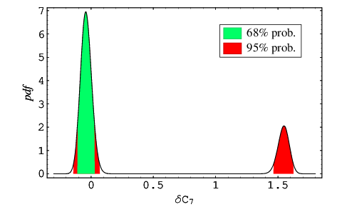
As far the sign of C7C_{7} is concerned, we find that the wrong sign solution to C7C_{7} is still allowed, but has a lower probability compared to the SM sign. As shown in Fig. 2, the large contribution to δ​C7\delta C_{7}, corresponding to a sign flip of C7​(mb)C_{7}(m_{b}), has a probability of about 30%. We stress that the sign flip of C7​(mb)C_{7}(m_{b}) occurs only if C9C_{9} receives a sizable non-standard contribution. This is consistent with the conclusion of Ref. [60], where the wrong sign solution to C7C_{7} has been excluded assuming small new-physics effects in the other Wilson coefficients.

Refer to caption
Refer to caption
Refer to caption
Figure 1: Correlation plots for the pairs of shifts in the Wilson coefficients. Allowed regions at 68% (in green) and 95% (in red) probability.
Refer to caption
Figure 2: Probability distribution of δ​C7\delta C_{7}.

The impact of the low- and high-energy regions in B→Xs​ℓ+​ℓ−B\to X_{s}\ell^{+}\ell^{-}, which are often neglected, can be seen in Fig. 3, where we plot the most interesting 68% and 95% allowed regions with or without the information of these two measurements. In view of future experimental improvements, we report below the numerical values of the main observables expanded in powers of the δ​Ci\delta C_{i}:

ℬ⁡(B→Xs​γ)​(Eγ>1.6​GeV)=3.13​(23)×10−4×(1−2.28​δ​C7+1.51​δ​C72),\displaystyle\mathcal{B}(B\to X_{s}\gamma)(E_{\gamma}>1.6\mathrm{GeV})=3.13(23)\times 10^{-4}\times(1-2.28\delta C_{7}+1.51\delta C_{7}^{2})\,, (40)
ℬ⁡(B→Xs​ℓ+​ℓ−)​(q2∈[0.0021,0.04]​GeV2)=0.8​(2)×10−6\displaystyle\mathcal{B}(B\to X_{s}\ell^{+}\ell^{-})(q^{2}\in[0.0021,0.04]~\mathrm{GeV}^{2})=0.8(2)\times 10^{-6}
×[1+2.02δC72+0.20δC92+0.20δC102−2.23δC7+0.23δC9−0.37δC10+0.31δC7δC9\displaystyle\hskip 28.45274pt\times\left[1+2.02\delta C_{7}^{2}+0.20\delta C_{9}^{2}+0.20\delta C_{10}^{2}-2.23\delta C_{7}+0.23\delta C_{9}-0.37\delta C_{10}+0.31\delta C_{7}\delta C_{9}\right.
+0.01(δCSμ)2−0.01δC10δCSμ+0.01δCSμ]\displaystyle\hskip 28.45274pt\left.+0.01(\delta C^{\mu}_{S})^{2}-0.01\delta C_{10}\delta C^{\mu}_{S}+0.01\delta C^{\mu}_{S}\right]\,
ℬ⁡(B→Xs​ℓ+​ℓ−)​(q2∈[1.0,6.0]​GeV2)=1.6​(1)×10−6\displaystyle\mathcal{B}(B\to X_{s}\ell^{+}\ell^{-})(q^{2}\in[1.0,6.0]~\mathrm{GeV}^{2})=1.6(1)\times 10^{-6}
×[1+0.64δC72+0.61δC92+0.61δC102−0.03δC7+0.86δC9−1.15δC10+0.73δC7δC9\displaystyle\hskip 28.45274pt\times\left[1+0.64\delta C_{7}^{2}+0.61\delta C_{9}^{2}+0.61\delta C_{10}^{2}-0.03\delta C_{7}+0.86\delta C_{9}-1.15\delta C_{10}+0.73\delta C_{7}\delta C_{9}\right.
+0.13(δCSμ)2−0.03δC10δCSμ+0.04δCSμ],\displaystyle\hskip 28.45274pt\left.+0.13(\delta C^{\mu}_{S})^{2}-0.03\delta C_{10}\delta C^{\mu}_{S}+0.04\delta C^{\mu}_{S}\right]\,,
ℬ⁡(B→Xs​ℓ+​ℓ−)​(q2∈[14.4,25.0]​GeV2)=2.3​(7)×10−7\displaystyle\mathcal{B}(B\to X_{s}\ell^{+}\ell^{-})(q^{2}\in[14.4,25.0]~\mathrm{GeV}^{2})=2.3(7)\times 10^{-7}
×[1+0.05δC72+0.28δC7+0.59δC92+0.59δC102+1.04δC9−1.13δC10+0.32δC7δC9\displaystyle\hskip 28.45274pt\times\left[1+0.05\delta C_{7}^{2}+0.28\delta C_{7}+0.59\delta C_{9}^{2}+0.59\delta C_{10}^{2}+1.04\delta C_{9}-1.13\delta C_{10}+0.32\delta C_{7}\delta C_{9}\right.
+0.27(δCSμ)2−0.02δC10δCSμ+0.02δCSμ],\displaystyle\hskip 28.45274pt\left.+0.27(\delta C^{\mu}_{S})^{2}-0.02\delta C_{10}\delta C^{\mu}_{S}+0.02\delta C^{\mu}_{S}\right]\,, (41)
ℬ⁡(Bs→μ+​μ−)\displaystyle\mathcal{B}(B_{s}\to\mu^{+}\mu^{-}) =\displaystyle= 4.1​(8)×10−9×[(1−1.04​δ​C10−29.3​δ​CSμ)2+860​(δ​CSμ)2],\displaystyle 4.1(8)\times 10^{-9}\times\left[(1-1.04\delta C_{10}-29.3\delta C^{\mu}_{S})^{2}+860(\delta C^{\mu}_{S})^{2}\right]\,, (42)
ℬ⁡(K+→π+​ν​ν¯)\displaystyle\mathcal{B}(K^{+}\to\pi^{+}\nu\bar{\nu}) =\displaystyle= 8.6​(9)×10−11​[1+0.96​δ​Cν​ν¯+0.24​δ​Cν​ν¯2].\displaystyle 8.6(9)\times 10^{-11}\left[1+0.96\delta C_{\nu\bar{\nu}}+0.24\delta C_{\nu\bar{\nu}}^{2}\right]\,. (43)
Refer to caption
Refer to caption
Figure 3: Correlation plots for the pairs of shifts in the Wilson coefficients, which are most affected by including the low and high energy regions in B→Xs​ℓ+​ℓ−B\to X_{s}\ell^{+}\ell^{-}. The left plot shows regions allowed at 68% (in green) while in the right plot, the regions shown are allowed at 95% (in red). The dark and light shaded regions correspond to the fit with and without the low and high energy regions in B→Xs​ℓ+​ℓ−B\to X_{s}\ell^{+}\ell^{-} respectively.

Since the experimental information of exclusive B→K∗​ℓ+​ℓ−B\to K^{*}\ell^{+}\ell^{-} modes is quite good [27], we have also investigated the impact of including these observables in the fit. In this case we have used the results of Ref. [31] for the hadronic form factors and their corresponding errors, taking into account additional theoretical uncertainty due to neglected additional long distance effects [28, 29, 30].

The FB asymmetry plays a significant role. In particular, the normalised FB asymmetry

𝒜¯FB​(q2)=1d​Γ/d​q2​d​𝒜FBd​q2\bar{\cal A}_{\rm FB}(q^{2})=\frac{1}{{\rm d}\Gamma/{\rm d}q^{2}}\frac{{\rm d}{\cal A}_{\rm FB}}{{\rm d}q^{2}} (44)

is interesting since the main uncertainty due to the form factors, namely the overall normalization of the decay rate, partly cancels out. Moreover, AF​B​(B→K∗​ℓ+​ℓ−)A_{FB}(B\to K^{*}\ell^{+}\ell^{-}) in the low q2q^{2} energy region is very small in the SM due to the destructive interference of C7C_{7} and C9C_{9} (resulting in the famous zero of the asymmetry at low q2q^{2}). It is therefore a good probe of the relative sign of the Wilson coefficients. The impact of including the presently available data on 𝒜FB​(B→K∗​ℓ+​ℓ−){\cal A}_{\rm FB}(B\to K^{*}\ell^{+}\ell^{-}) is shown in Fig. 4.77 7 AF​B​(B→K∗​ℓ+​ℓ−)A_{FB}(B\to K^{*}\ell^{+}\ell^{-}) has been measured both by Belle [61] and Babar [27]. However, in Ref. [61] only the fully integrated asymmetry has been reported. The normalised values of AF​B​(B→K∗​ℓ+​ℓ−)A_{FB}(B\to K^{*}\ell^{+}\ell^{-}) in different q2q^{2} bins, as reported in Ref. [27], represent the most useful information for our purpose. For this reason, we have restricted our numerical analysis only to the results in Ref. [27]. As can be seen, at present the additional information significantly reduces part of the ambiguities in the δ​C9\delta C_{9}–δ​C10\delta C_{10} and δ​C10\delta C_{10}–δ​C0μ\delta C^{\mu}_{0} planes only at 68%68\% probability level. On the other hand, the overall bounds on the scales of individual coefficients do not change in appreciable way. This may seem at odds with conclusions reached in refs. [27, 61]. However, the central experimental values for the high q2q^{2} region lie approximately 1.5 standard deviations above the range of possible theory predicitions within MFV satisfying other bounds. In addition, this range of theory predictions spans less than two experimental standard deviations. Under the assumption of MFV validity, the present FB asymmetry measurements therefore cannot significantly affect the 95%95\% probability regions of δ​Ci\delta C_{i}. As seen on Fig. 4, the situation would however improve dramatically, once the experimental precision would approximately double.

Contrary to the FB asymmetry, it turns out that the K∗K^{*} longitudinal polarization is not very sensitive to new physics in the MFV scenario.

Refer to caption
Refer to caption
Figure 4: Correlation plots for the pairs of shifts in the Wilson coefficients, which are most affected by including the exclusive AF​BA_{FB} observables. Allowed regions at 68% with (dark green) and without (light green) exclusive AF​BA_{FB} observables are shown.

For completeness, we report below the numerical expressions of AF​B​(B→K∗​ℓ+​ℓ−)A_{FB}(B\to K^{*}\ell^{+}\ell^{-}), integrated and normalised to the decay rate as in Ref. [27] expanded in powers of the δ​Ci\delta C_{i}:

𝒜FB​(B→K∗​ℓ+​ℓ−)q2<6.25​GeV2Γ​(B→K∗​ℓ+​ℓ−)q2<6.25​GeV2=−0.01(2)×\displaystyle\frac{\mathcal{A}_{\rm FB}(B\to K^{*}\ell^{+}\ell^{-})_{q^{2}<6.25~\mathrm{GeV}^{2}}}{\Gamma(B\to K^{*}\ell^{+}\ell^{-})_{q^{2}<6.25~\mathrm{GeV}^{2}}}=-0.01(2)\times
×(1−20.δC7−11.δC9+1.δC10+21.δC7δC10+11.δC9δC10)(1+1.2​δ​C72−0.7​δ​C7+0.5​δ​C92+0.5​δ​C102+0.6​δ​C9−1.0​δ​C10+0.8​δ​C7​δ​C9),\displaystyle\hskip 28.45274pt\times\frac{(1-20.\delta C_{7}-11.\delta C_{9}+1.\delta C_{10}+21.\delta C_{7}\delta C_{10}+11.\delta C_{9}\delta C_{10})}{(1+1.2\delta C_{7}^{2}-0.7\delta C_{7}+0.5\delta C_{9}^{2}+0.5\delta C_{10}^{2}+0.6\delta C_{9}-1.0\delta C_{10}+0.8\delta C_{7}\delta C_{9})}\,,
𝒜FB​(B→K∗​ℓ+​ℓ−)q2>10.24​GeV2Γ​(B→K∗​ℓ+​ℓ−)q2>10.24​GeV2=0.20(8)×\displaystyle\frac{\mathcal{A}_{\rm FB}(B\to K^{*}\ell^{+}\ell^{-})_{q^{2}>10.24~\mathrm{GeV}^{2}}}{\Gamma(B\to K^{*}\ell^{+}\ell^{-})_{q^{2}>10.24~\mathrm{GeV}^{2}}}=0.20(8)\times
×(1+0.5​δ​C7+1.2​δ​C9−1.0​δ​C10−0.5​δ​C7​δ​C10−1.3​δ​C9​δ​C10)(1+0.1​δ​C72+0.4​δ​C7+0.6​δ​C92+0.6​δ​C102+1.0​δ​C9−1.2​δ​C10+0.4​δ​C7​δ​C9).\displaystyle\hskip 28.45274pt\times\frac{(1+0.5\delta C_{7}+1.2\delta C_{9}-1.0\delta C_{10}-0.5\delta C_{7}\delta C_{10}-1.3\delta C_{9}\delta C_{10})}{(1+0.1\delta C_{7}^{2}+0.4\delta C_{7}+0.6\delta C_{9}^{2}+0.6\delta C_{10}^{2}+1.0\delta C_{9}-1.2\delta C_{10}+0.4\delta C_{7}\delta C_{9})}\,.\qquad (45)

In the above expressions, we have neglected the scalar operator contributions, which are made negligible by the strong bound coming from Bs→μ+​μ−B_{s}\to\mu^{+}\mu^{-}. However, δ​CSμ\delta C^{\mu}_{S} dominates possible NP effects in the lepton universality ratios of B→K(∗)​ℓ+​ℓ−B\to K^{(*)}\ell^{+}\ell^{-}, as we discuss in the next section.

5 Predictions
Refer to caption
Refer to caption
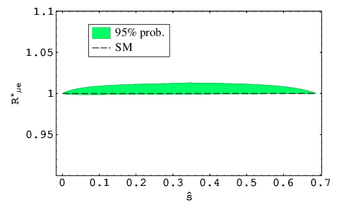
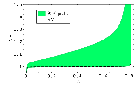
Figure 5: 95% probability allowed ranges for the lepton universality ratio (muon/electron) for the differential distributions of B→K​ℓ+​ℓ−B\to K\ell^{+}\ell^{-} (left) and B→K∗​ℓ+​ℓ−B\to K^{*}\ell^{+}\ell^{-} (right).

Using the bounds on the MFV operators discussed in the previous section, we obtain a series of constraints for FCNC processes which are not well measured yet. The most interesting predictions can be summarised as follows:
Refer to caption
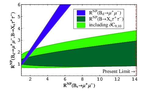
Figure 6: Correlations between Bs→μ+​μ−B_{s}\to\mu^{+}\mu^{-}, Bd→μ+​μ−B_{d}\to\mu^{+}\mu^{-}, and Bs→Xs​τ+​τ−B_{s}\to X_{s}\tau^{+}\tau^{-}. For a given value of ℬ⁡(Bs→μ+​μ−)\mathcal{B}(B_{s}\to\mu^{+}\mu^{-}), normalised to the SM prediction (horizonatal axis), we plot the range of ℬ⁡(Bd→μ+​μ−)\mathcal{B}(B_{d}\to\mu^{+}\mu^{-}) and ℬ⁡(Bs→Xs​μ+​μ−)\mathcal{B}(B_{s}\to X_{s}\mu^{+}\mu^{-}), both normalised to the correponding SM predictions (vertical axis).
  • •

    R(μ/e)​(B→K(∗)​ℓ+​ℓ−)R^{(\mu/e)}(B\to K^{(*)}\ell^{+}\ell^{-}).
    As pointed out in Ref. [51] the lepton universality ratios (or the muon to electron ratios of branching ratios) in B→K(∗)​ℓ+​ℓ−B\to K^{(*)}\ell^{+}\ell^{-} are very clean probes of possible scalar density operators. Within the MFV framework there is a one-to-one correspondence between possible deviations from the SM in the lepton universality ratios and the contribution of the scalar-density operator in Bs→μ+​μ−B_{s}\to\mu^{+}\mu^{-}. Thanks to the substantial improvement on Bs→μ+​μ−B_{s}\to\mu^{+}\mu^{-}, the effect is highly constrained.

    The present allowed ranges for the differential distributions of the lepton universality ratios are shown in Fig. 5. As can be seen, the effect is negligibly small in the B→K∗B\to K^{*} case. In the B→KB\to K case there is still some room for deviations from the SM, but only in the high-q2q^{2} region, where the decay is suppressed. The maximal integrated effect is reported in Table 6. Note the major improvement with respect to the analysis of Ref. [51], where the loose bound on Bs→μ+​μ−B_{s}\to\mu^{+}\mu^{-} allowed much larger non-standard effects.

  • •

    ℬ⁡(Bd→μ+​μ−)\mathcal{B}(B_{d}\to\mu^{+}\mu^{-})
    As anticipated, probably the best test of the MFV scenario in the Δ​F=1\Delta F=1 sector is the ratio in Eq. (36). Taking into account the present bound on Bs→μ+​μ−B_{s}\to\mu^{+}\mu^{-} this implies the upper limit

    ℬ⁡(Bd→μ+​μ−)<1.2×10⁻⁹,\mathcal{B}(B_{d}\to\mu^{+}\mu^{-})<1.2\times 10^{-9}~, (46)

    at 95% probability. The clear correlation between ℬ⁡(Bd→μ+​μ−)\mathcal{B}(B_{d}\to\mu^{+}\mu^{-}) and ℬ⁡(Bs→μ+​μ−)\mathcal{B}(B_{s}\to\mu^{+}\mu^{-}) in the MFV framework is illustrated in Fig. 6.

  • •

    ℬ⁡(B→Xs​τ+​τ−)\mathcal{B}(B\to X_{s}\tau^{+}\tau^{-})
    The bound on the scalar-current operator allows us to derive a non-trivial bound also on ℬ⁡(B→Xs​τ+​τ−)\mathcal{B}(B\to X_{s}\tau^{+}\tau^{-}), which at large tan⁡β\tan\beta is sensitive to scalar-current operators. The parametrical dependence on the modified Wilson coefficient of the integrated branching ratio is

    ℬ​(B→Xs​τ+​τ−)q2∈[14.4,25.0]​GeV2\displaystyle\mathcal{B}(B\to X_{s}\tau^{+}\tau^{-})_{q^{2}\in[14.4,25.0]~\mathrm{GeV}^{2}} =\displaystyle= 1.6​(5)×10−7\displaystyle 1.6(5)\times 10^{-7} (47)
    ×(1+0.06​δ​C72+0.38​δ​C7+0.81​δ​C92+0.41​δ​C102+1.41​δ​C9CLOSE\displaystyle\hskip-170.71652pt\times(1+0.06\delta C_{7}^{2}+0.38\delta C_{7}+0.81\delta C_{9}^{2}+0.41\delta C_{10}^{2}+1.41\delta C_{9}
    OPEN−0.78​δ​C10+0.43​δ​C7​δ​C9−0.54​δ​C10​δ​CSτ+0.52​δ​CSτ+0.32​δ​CSτ2).\displaystyle\hskip-170.71652pt-0.78\delta C_{10}+0.43\delta C_{7}\delta C_{9}-0.54\delta C_{10}\delta C^{\tau}_{S}+0.52\delta C^{\tau}_{S}+0.32{\delta C^{\tau}_{S}}^{2})\,.

    Assuming δ​CSτ=(mτ/mμ)​δ​CSμ\delta C^{\tau}_{S}=(m_{\tau}/m_{\mu})\delta C^{\mu}_{S}, in agreement with Eq. (6), and taking into account the allowed ranges of the Wilson coefficients in Table  4, we obtain the 95%95\% probability bound reported in Table 6.

  • •

    d​AF​B/d​q2​(B→Xs​ℓ+​ℓ−)\mathrm{d}A_{FB}/\mathrm{d}q^{2}(B\to X_{s}\ell^{+}\ell^{-})
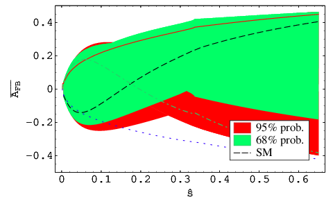
    Taking into account the available constraints on C7,9,10C_{7,9,10}, the resulting allowed range for the inclusive FB asymmetry is shown in Fig. 7. As can be seen, in this case there is still a large room for non-standard effects: this observable is one of the few examples of quantities which could exhibit large deviations from the SM even in the pessimistic MFV framework. On the other hand, present data exclude most confgurations with flipped sgn(C9/C10C_{9}/C_{10}) at 68%68\% probability.

  • •

    ℬ⁡(B→K(∗)​ν​ν¯)\mathcal{B}(B\to K^{(*)}\nu\bar{\nu}) and ℬ⁡(KL→π0​ν​ν¯)\mathcal{B}(K_{L}\to\pi^{0}\nu\bar{\nu})
    From the K+→ν​ν¯K^{+}\to\nu\bar{\nu} bound on δ​Cν​ν\delta C_{\nu\nu} we can bound the rates of all the ν​ν¯\nu\bar{\nu}-type FCNC transitions88 8 These predictions are valid only in the limit where we can neglect operators with the Yu†​Yu​Yd†​YdY_{u}^{\dagger}Y_{u}Y_{d}^{\dagger}Y_{d} flavour structure. This condition is always fullfiled at small/moderate tan⁡β\tan\beta and even at large tan⁡β\tan\beta holds in most excplicit MFV scenarios.. The most interesting predictions are reported in Table 6 (in the ℬ⁡(B→K(∗)​ν​ν¯)\mathcal{B}(B\to K^{(*)}\nu\bar{\nu}) case we take into account form-factor uncertainties along the lines discussed in Section 3.2). For completeness, we give the numerical expressions of the KL→π0​ν​ν¯K_{L}\to\pi^{0}\nu\bar{\nu} and B→K(∗)​ν​ν¯B\to K^{(*)}\nu\bar{\nu} branching ratios:

    ℬ⁡(KL→π0​ν​ν¯)\displaystyle\mathcal{B}(K_{L}\to\pi^{0}\nu\bar{\nu}) =\displaystyle= 2.9​(5)×10−11​[1+1.37​δ​Cν​ν¯+0.47​δ​Cν​ν¯2],\displaystyle 2.9(5)\times 10^{-11}\left[1+1.37\delta C_{\nu\bar{\nu}}+0.47\delta C_{\nu\bar{\nu}}^{2}\right]\,,
    ℬ⁡(B→K​ν​ν¯)\displaystyle\mathcal{B}(B\to K\nu\bar{\nu}) =\displaystyle= 0.5​(1)×10−5​[1+1.2​δ​Cν​ν¯+0.4​δ​Cν​ν¯2],\displaystyle 0.5(1)\times 10^{-5}\left[1+1.2\delta C_{\nu\bar{\nu}}+0.4\delta C_{\nu\bar{\nu}}^{2}\right]\,,
    ℬ⁡(B→K∗​ν​ν¯)\displaystyle\mathcal{B}(B\to K^{*}\nu\bar{\nu}) =\displaystyle= 1.2​(3)×10−5​[1+1.2​δ​Cν​ν¯+0.4​δ​Cν​ν¯2].\displaystyle 1.2(3)\times 10^{-5}\left[1+1.2\delta C_{\nu\bar{\nu}}+0.4\delta C_{\nu\bar{\nu}}^{2}\right]\,. (48)
Observable Experiment MFV bound SM prediction
R(μ/e)​(B→K​ℓ+​ℓ−)−1R^{(\mu/e)}(B\to K\ell^{+}\ell^{-})-1 0.17±0.280.17\pm 0.28 [62, 63]99 9 Here we quote naïve averages of the values obtained by the experiments and with symmetrized errors. [−0.004,0.14][-0.004,0.14] O⁡(10−4)O(10^{-4}) [64]
R(μ/e)​(B→K∗​ℓ+​ℓ−)−1R^{(\mu/e)}(B\to K^{*}\ell^{+}\ell^{-})-1 0.37−0.40+0.53±0.090.37^{+0.53}_{-0.40}\pm 0.09 [63] [−0.002,0.01][-0.002,0.01] ∼<10−2\stackrel{{\scriptstyle<}}{{{}_{\sim}}}10^{-2}
ℬ⁡(Bd→μ+​μ−)\mathcal{B}(B_{d}\to\mu^{+}\mu^{-}) <1.8×10⁻⁸<1.8\times 10^{-8} [24] <1.2×10⁻⁹<1.2\times 10^{-9} 1.3​(3)×10−101.3(3)\times 10^{-10}
ℬ⁡(B→Xs​τ+​τ−)\mathcal{B}(B\to X_{s}\tau^{+}\tau^{-}) – <5×10⁻⁷<5\times 10^{-7} 1.6​(5)×10−71.6(5)\times 10^{-7}
ℬ⁡(B→K​ν​ν¯)\mathcal{B}(B\to K\nu\bar{\nu}) [65] <0.4×10⁻⁴<0.4\times 10^{-4} (0.5±0.1)×10−5(0.5\pm 0.1)\times 10^{-5}
ℬ⁡(B→K∗​ν​ν¯)\mathcal{B}(B\to K^{*}\nu\bar{\nu}) [65] <9.4×10⁻⁵<9.4\times 10^{-5} (1.2±0.3)×10−5(1.2\pm 0.3)\times 10^{-5}
ℬ⁡(KL→π0​ν​ν¯)\mathcal{B}(K_{L}\to\pi^{0}\nu\bar{\nu}) [66] <2.9×10⁻¹⁰<2.9\times 10^{-10} 2.9​(5)×10−112.9(5)\times 10^{-11}
Table 6: Predicted observables. All bounds are 95% probability limits. In the first two lines, the SM predictions refer to the kinematical region where lepton-mass phase-space effects can be safely neglected. The experimental results on ν​ν¯\nu\bar{\nu} modes are not explicilty indicated since only 90% C.L. limits are available.
Refer to caption
Refer to caption
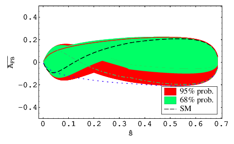
Figure 7: 95% probability allowed range for the inclusive normalised FB asymmetry in B→Xs​ℓ+​ℓ−B\to X_{s}\ell^{+}\ell^{-} (left) and B→K∗​ℓ+​ℓ−B\to K^{*}\ell^{+}\ell^{-} (right). The dashed curve denotes the central value of the SM prediction. The other three lines indicate the central values obtained flipping sgn(C7/C10C_{7}/C_{10}) and/or sgn(C9/C10C_{9}/C_{10}).

6 Conclusions

The MFV hypothesis provides an efficient tool to analyse flavour-violating effects in extensions of the SM. The effective theory built on this symmetry and and symmetry-breaking hypothesis leads to: 1) a natural suppression of flavour violating effects, in agreement with present observations, even for for new physics in the TeV range; 2) a series of experimentally testable predictions, which could help to identify the underlying mechanism of flavour symmetry breaking.

In this paper we have presented a general analysis of the MFV effective theory in the Δ​F=1\Delta F=1 sector. From the current stringent bounds on possible deviations from the SM in various BB-physics observables we have derived the bounds on the scale of new-physics reported in Table 5. As can be seen, these bounds are perfectly compatible with new dynamics in the TeV range. We recall that the in models where new particles contribute to FCNC processes only at the loop level, the bounds on the particle masses are one order of magnitude weaker with respect to the the bounds reported in Table 5: Λ∼4​π​mNP\Lambda\sim 4\pi m_{\rm NP}. Thus in weakly-interacting theories respcting the MFV hypothesis and with no tree-level FCNC, we could expect new particles well within the reach of the LHC.

Using the bounds on the effective operators, taking into account the correlations implied by the observables measured so far, we have derived a series of predictions for future high-statistics studies of flavour physics. This has allowed us to identify observables which could still exhibit large deviations for the SM even under the pessimistic hypothesis of MFV. The most interesting ones are the rare decays Bs,d→μ+​μ−B_{s,d}\to\mu^{+}\mu^{-}, rare BB and KK decays with a neutrino pair in the final state, and the FB asymmetry in B→K∗​ℓ+​ℓ−B\to K^{*}\ell^{+}\ell^{-} decays. The allowed parameter space for the latter is shown in Fig. 7.

Using the current bounds on MFV operators we have also identified a series of stringent tests of this symmetry principle. The most interesting negative predictions are summarised in Table 6. If these predictions were falsified by future experiments, we could unambiguously conclude that there exist new flavour symmetry-breaking structures beyond the SM Yukawa couplings. The effective theory allows us to obtain also some positive predictions, namely correlations among different observables which could still exhibit a deviation form the SM. The most interesting of such positive predictions is the correlation between Bs→μ+​μ−B_{s}\to\mu^{+}\mu^{-} and Bd→μ+​μ−B_{d}\to\mu^{+}\mu^{-} implied by Eq. (36) and illustrated in Fig. 6. A clear evidence of physics beyond the SM in both channels, respecting this correlation, would provide a strong support of the MFV hypothesis.

Acknowledgements

We thank J. Charles, S. Descotes-Genon and U. Haisch for interesting discussions, and D. Guadagnoli for his comments on the manuscript. This work is supported by the EU under contract MTRN-CT-2006-035482 Flavianet.

References

  • [1] G. D’Ambrosio, G. F. Giudice, G. Isidori and A. Strumia, Nucl. Phys. B 645 (2002) 155 [arXiv:hep-ph/0207036].
  • [2] R. S. Chivukula and H. Georgi, Phys. Lett. B 188 (1987) 99.
  • [3] A. J. Buras, et al. Phys. Lett. B 500 (2001) 161 [arXiv:hep-ph/0007085].
  • [4] A. Ali and D. London, Eur. Phys. J. C 9 (1999) 687 [arXiv:hep-ph/9903535]; A. J. Buras, Acta Phys. Polon. B 34 (2003) 5615 [arXiv:hep-ph/0310208]; B. Grinstein, V. Cirigliano, G. Isidori and M. B. Wise, Nucl. Phys. B 763 (2007) 35 [arXiv:hep-ph/0608123].
  • [5] E. Gabrielli and G. F. Giudice, Nucl. Phys. B 433, 3 (1995) [Erratum-ibid. B 507, 549 (1997)] [arXiv:hep-lat/9407029]; L. J. Hall and L. Randall, Phys. Rev. Lett. 65 (1990) 2939.
  • [6] P. Paradisi, M. Ratz, R. Schieren and C. Simonetto, arXiv:0805.3989 [hep-ph]; G. Colangelo, E. Nikolidakis and C. Smith, arXiv:0807.0801 [hep-ph]; B. Dudley and C. Kolda, arXiv:0805.4565 [hep-ph].
  • [7] E. Nikolidakis and C. Smith, Phys. Rev. D 77, 015021 (2008) [arXiv:0710.3129 [hep-ph]].
  • [8] G. Cacciapaglia, C. Csaki, J. Galloway, G. Marandella, J. Terning and A. Weiler, JHEP 0804 (2008) 006 [arXiv:0709.1714 [hep-ph]].
  • [9] M. Bona et al. [UTfit Collaboration], JHEP 0803 (2008) 049 [arXiv:0707.0636 [hep-ph]]; for UT angle γ\gamma we use the updated value on http://www.utfit.org/.
  • [10] E. Barberio et al. [Heavy Flavor Averaging Group (HFAG) Collaboration], arXiv:0704.3575 [hep-ex], and online update at http://www.slac.stanford.edu/xorg/hfag
  • [11] M. Misiak et al., Phys. Rev. Lett. 98, 022002 (2007) [arXiv:hep-ph/0609232].
  • [12] M. Misiak and M. Steinhauser, Nucl. Phys. B 764 (2007) 62 [arXiv:hep-ph/0609241].
  • [13] U. Haisch, arXiv:0805.2141 [hep-ph].
  • [14] M. Iwasaki et al. [Belle Collaboration], Phys. Rev. D 72, 092005 (2005) [arXiv:hep-ex/0503044].
  • [15] B. Aubert et al. [BABAR Collaboration], Phys. Rev. Lett. 93, 081802 (2004) [arXiv:hep-ex/0404006].
  • [16] C. Bobeth, M. Misiak and J. Urban, Nucl. Phys. B 574, 291 (2000) [arXiv:hep-ph/9910220].
  • [17] H. H. Asatryan, H. M. Asatrian, C. Greub and M. Walker, Phys. Rev. D 65 (2002) 074004 [arXiv:hep-ph/0109140].
  • [18] H. M. Asatrian, K. Bieri, C. Greub and A. Hovhannisyan, Phys. Rev. D 66, 094013 (2002) [arXiv:hep-ph/0209006].
  • [19] A. Ghinculov, T. Hurth, G. Isidori and Y. P. Yao, Nucl. Phys. B 685, 351 (2004) [arXiv:hep-ph/0312128].
  • [20] C. Bobeth, P. Gambino, M. Gorbahn and U. Haisch, JHEP 0404, 071 (2004) [arXiv:hep-ph/0312090].
  • [21] T. Huber, E. Lunghi, M. Misiak and D. Wyler, Nucl. Phys. B 740, 105 (2006) [arXiv:hep-ph/0512066].
  • [22] T. Huber, T. Hurth and E. Lunghi, arXiv:0712.3009 [hep-ph].
  • [23] Z. Ligeti and F. J. Tackmann, Phys. Lett. B 653 (2007) 404 [arXiv:0707.1694 [hep-ph]].
  • [24] T. Aaltonen et al. [CDF Collaboration], Phys. Rev. Lett. 100 (2008) 101802 [arXiv:0712.1708 [hep-ex]].
  • [25] G. Buchalla, A. J. Buras and M. E. Lautenbacher, Rev. Mod. Phys. 68 (1996) 1125 [arXiv:hep-ph/9512380].
  • [26] Q. Mason et al. [HPQCD Collaboration and UKQCD Collaboration], Phys. Rev. Lett. 95, 052002 (2005) [arXiv:hep-lat/0503005]; C. Bernard et al. [Fermilab Lattice, MILC and HPQCD Collaborations], PoS LATTICE2007, 370 (2007).
  • [27] B. Aubert et al. [BABAR Collaboration], arXiv:0804.4412 [hep-ex]; Phys. Rev. D 73, 092001 (2006) [arXiv:hep-ex/0604007].
  • [28] M. Beneke, T. Feldmann and D. Seidel, Nucl. Phys. B 612, 25 (2001) [arXiv:hep-ph/0106067].
  • [29] M. Beneke, T. Feldmann and D. Seidel, Eur. Phys. J. C 41 (2005) 173 [arXiv:hep-ph/0412400].
  • [30] A. Ali, G. Kramer and G. h. Zhu, Eur. Phys. J. C 47 (2006) 625 [arXiv:hep-ph/0601034].
  • [31] P. Ball and R. Zwicky, Phys. Rev. D 71 (2005) 014029 [arXiv:hep-ph/0412079].
  • [32] S. Adler et al. [E787 Collaboration], Phys. Rev. D 77 (2008) 052003; V. V. Anisimovsky et al. [E949 Collaboration], Phys. Rev. Lett. 93 (2004) 031801 [arXiv:hep-ex/0403036].
  • [33] M. Antonelli et al. [FlaviaNet Working Group on Kaon Decays], arXiv:0801.1817 [hep-ph] and online update at http://www.lnf.infn.it/wg/vus/ from Rare K decays and Decay Constants.
  • [34] J. Brod and M. Gorbahn, arXiv:0805.4119 [hep-ph].
  • [35] A. J. Buras, M. Gorbahn, U. Haisch and U. Nierste, JHEP 0611, 002 (2006) [arXiv:hep-ph/0603079]; Phys. Rev. Lett. 95, 261805 (2005) [arXiv:hep-ph/0508165].
  • [36] G. Isidori, F. Mescia and C. Smith, Nucl. Phys. B 718, 319 (2005) [arXiv:hep-ph/0503107].
  • [37] F. Mescia and C. Smith, Phys. Rev. D 76, 034017 (2007) [arXiv:0705.2025 [hep-ph]].
  • [38] A. J. Buras, Phys. Lett. B 566, 115 (2003) [arXiv:hep-ph/0303060].
  • [39] C. Bobeth, M. Bona, A. J. Buras, T. Ewerth, M. Pierini, L. Silvestrini and A. Weiler, Nucl. Phys. B 726 (2005) 252 [arXiv:hep-ph/0505110].
  • [40] U. Haisch and A. Weiler, Phys. Rev. D 76, 074027 (2007) [arXiv:0706.2054 [hep-ph]].
  • [41] K. S. Babu and C. F. Kolda, Phys. Rev. Lett. 84 (2000) 228 [arXiv:hep-ph/9909476].
  • [42] G. Isidori and A. Retico, JHEP 0111 (2001) 001 [arXiv:hep-ph/0110121].
  • [43] W. Altmannshofer, A. J. Buras and D. Guadagnoli, JHEP 0711 (2007) 065 [arXiv:hep-ph/0703200].
  • [44] P. Gambino, M. Gorbahn and U. Haisch, Nucl. Phys. B 673 (2003) 238 [arXiv:hep-ph/0306079].
  • [45] M. Gorbahn and U. Haisch, Nucl. Phys. B 713, 291 (2005) [arXiv:hep-ph/0411071].
  • [46] G. Buchalla, G. Isidori and S. J. Rey, Nucl. Phys. B 511 (1998) 594 [arXiv:hep-ph/9705253].
  • [47] S. J. Lee, M. Neubert and G. Paz, Phys. Rev. D 75 (2007) 114005 [arXiv:hep-ph/0609224].
  • [48] T. Huber, T. Hurth and E. Lunghi, arXiv:0807.1940 [hep-ph].
  • [49] P. Ball and R. Zwicky, JHEP 0110 (2001) 019 [arXiv:hep-ph/0110115].
  • [50] A. Ali, P. Ball, L. T. Handoko and G. Hiller, Phys. Rev. D 61 (2000) 074024 [arXiv:hep-ph/9910221].
  • [51] G. Hiller and F. Kruger, Phys. Rev. D 69, 074020 (2004) [arXiv:hep-ph/0310219].
  • [52] R. J. Hill, T. Becher, S. J. Lee and M. Neubert, JHEP 0407 (2004) 081 [arXiv:hep-ph/0404217].
  • [53] U. Egede, T. Hurth, J. Matias, M. Ramon and W. Reece, arXiv:0807.2589 [hep-ph].
  • [54] P. Ball and R. Zwicky, Phys. Rev. D 71 (2005) 014015 [arXiv:hep-ph/0406232].
  • [55] G. Buchalla, G. Hiller and G. Isidori, Phys. Rev. D 63 (2001) 014015 [arXiv:hep-ph/0006136].
  • [56] P. Colangelo, F. De Fazio, R. Ferrandes and T. N. Pham, Phys. Rev. D 73 (2006) 115006 [arXiv:hep-ph/0604029].
  • [57] M. Misiak, private communication.
  • [58] W. M. Yao et al. [Particle Data Group], J. Phys. G 33, 1 (2006), and online update at http://pdg.lbl.gov/
  • [59] N. Tantalo, arXiv:hep-ph/0703241;S. Hashimoto, hep-ph/0411126; D. Becirevic, hep-ph/0310072.
  • [60] P. Gambino, U. Haisch and M. Misiak, Phys. Rev. Lett. 94, 061803 (2005) [arXiv:hep-ph/0410155].
  • [61] A. Ishikawa et al., Phys. Rev. Lett. 96 (2006) 251801 [arXiv:hep-ex/0603018].
  • [62] K. Abe et al. [Belle Collaboration], arXiv:hep-ex/0410006.
  • [63] B. Aubert [The BABAR Collaboration], arXiv:0807.4119 [hep-ex].
  • [64] C. Bobeth, G. Hiller and G. Piranishvili, JHEP 0712 (2007) 040 [arXiv:0709.4174 [hep-ph]].
  • [65] K. F. Chen et al. [BELLE Collaboration], Phys. Rev. Lett. 99 (2007) 221802 [arXiv:0707.0138 [hep-ex]]; B. Aubert et al. [BABAR Collaboration], Phys. Rev. Lett. 94 (2005) 101801 [arXiv:hep-ex/0411061].
  • [66] J. Nix et al. [E391a Collaboration], Phys. Rev. D 76 (2007) 011101 [arXiv:hep-ex/0701058].