Dynamical Analysis on Gene Activity in the Presence of Repressors and an Interfering Promoter

Hiizu Nakanishi, Namiko Mitarai, and Kim Sneppen Affiliation: Niels Bohr Institute, Blegdamsvej 17, Dk 2100, Copenhagen, Denmark Affiliation: Department of Physics, Kyushu University 33, Fukuoka 812-8582, Japan

August 24, 2026

Abstract

Detailed derivations for the mathematical expressions in the text are given.

Introduction

The regulation of the activity of a particular gene involves a complex interplay between a promoter, an RNA polymerase (RNAP), and one or several transcription factors (TF) [1, 2]. Ignoring the internal dynamics associated with transcription initiation, the probability for obtaining a successful RNAP elongation initiation can be estimated from an equilibrium unbinding ratio of TF[3, 4]. When internal steps in transcription initiations becomes sizeable we need to consider the race between these steps and the kinetics of TF binding.

The binding/unbinding rates of TF to bind to an operator is critically influenced by competitive non-specific bindings [5, 6]. Recent measurements of in vivo dynamics in an E. coli cell finds that a single lac repressor needs between 60 and 360 seconds to locate its operator [6]. For TF whose copy number is of the order of 10 to 100 per cell, a cleared operator can remain free for up to about 30 seconds. In comparison, RNAP transcription initiation rates varies considerably, and can be as fast as 1.8 transcription initiation per second for a certain ribosomal promoter [7]. Therefore, there is “room” for effects associated to the race between first bindings of a TF or an RNAP once the promoter is cleared.

In a number of both procaryotic and eucaryotic systems, the promoter activity are not only influenced by TF, but are also modulated by interfering promoters [8, 9, 10, 11, 12, 13, 14, 15]. For example, the regulation between lytic and lysogenic maintenance promoters in the P2 class of bacteriophages involves transcription interferences (TI) as well as TF’s that repress the promoter activities [11]. And in lambdoid phages the initial lysis-lysogeny decision is modulated by TI between the promoter PRE activated by CII and the promoter PR repressed by CI.

Dodd et al.[15] presented a framework to deal with TI and multiple TF’s, using an assumption about fast equilibrium reactions of TF-binding and closed complex formation. In the present paper, we develop a formalism that deals with the competition between time scales of TF binding/unbinding and transcription initiation process, and examine the effect of interference.

Refer to caption — Figure 1: (a) Model of promoter pS with a single TF that represses the promoter by competitive binding to an operator that overlaps with the promoter. The promoter activity is given in terms of the three-step Hawley-McClure model for transcription initiation, with indicated transition rates for formation of closed complex, that of open complex, and elongation. (b) Same as in (a), but with addition of a convergent promoter that interfere with both RNAP binding to pS and with binding of TF.

Fig.1 shows a single promoter pS with an operator site for a repressive TF (left panel), and with a convergent promoter pA (right panel). For both cases, we illustrate the three basic steps of transcription initiation: (i) RNAP reversible binding to form a closed complex, (ii) irreversible transition to open complex, and (iii) initiation of transcription elongation. The rates for these three steps are promoter dependent [16, 17, 18]. As for the initial binding, given the fact that the maximum activity for ribosomal promoters reaches 1.8 transcriptions per second[7], the time needed for an RNAP to diffuse to a promoter cannot be longer than $\sim 0.5$ sec. Regarding the later steps where RNAP forms open complex and subsequently initiates transcription to leave the promoter, their time scales may vary a great deal from one promoter to another[19, 20, 21, 22, 23].

In the following, we will investigate in detail how these time scales play together to determine the extent to which a promoter is sensitive to repressors and to clearance due to the interference by elongating RNAP’s from other promoters[24].

Models

We study the promoter activity under influence of transcription factor(TF) and transcription interference(TI) based on mathematical analysis on simple models of promoter in the following three levels. Our goal is to understand regulation of the three step model for transcription initiation originally proposed by Hawley-McClure[16, 17], but we also analyze its simplified versions, i.e. the single step model and the two step model. The comparison of these three levels of models gives us intuitive understanding of the promoter behavior.

Three Models for Elongation Initiation

Let us start by describing the bare models with neither TF nor TI (Fig.2).

i) The single step model of transcription initiation is the model where the whole process is dominated by a slowest step, thus its elongation initiation is represented by a simple Poissonian process with the rate $\Omega_{0}$ .

ii) In the two step model, the transcription initiation consists of two steps: first, RNAP binds to the promoter site with the on-rate $k_{\rm on}$ , and then initiates elongation with the rate $k_{e}$ . The transcription initiation rate for the overall process $\Omega_{0}$ is given by[14]

\Omega_{0}={k_{\rm on}k_{e}\over k_{\rm on}+k_{e}}={1\over\tau_{\rm on}+\tau_{e}}

(1)

with

\tau_{\rm on}\equiv{1\over k_{\rm on}},\quad\tau_{e}\equiv{1\over k_{e}}.

(2)

The last expression of (1) simply shows that the average interval of elongation initiation $1/\Omega_{0}$ is the sum of the two times: $\tau_{\rm on}$ , the time for RNAP to form the on-state, and $\tau_{e}$ , the time to start elongation in the on-state.

iii) In the three step model, two states within the RNAP binding state are differentiated: the one with closed DNA complex and the other with open DNA complex. The transition between the RNAP unbinding state (off-state) and the RNAP binding state with closed DNA is reversible, and characterized by the binding rate $k_{b}$ and the unbinding rate $k_{u}$ . When RNAP is in the closed complex state, the transition to the open state is irreversible with the rate $k_{o}$ . Finally, the open complex is followed by elongation initiation with the rate $k_{e}$ . This three step model of transcription initiation was originally proposed by Hawley-McClure[16, 17].

The three step model reduces to the two step model with the effective on-rate $k_{\rm on}^{*}$ given by

k_{\rm on}^{*}\equiv{k_{o}\over 1+k_{u}/k_{b}}

(3)

in the case where the off-state and the closed DNA binding state are in equilibrium. This is fulfilled when the initial reversible process of RNAP binding/unbinding is faster than the other processes: $k_{b}$ , $k_{u}\gg k_{o}$ , $k_{e}$ [14]. The effective on-rate $k_{\rm on}^{*}$ in eq.(3) can be understood as the open rate $k_{o}$ reduced by the equilibrium expectation of being unbound.

The overall elongation rate $\Omega_{0}$ for the three step model has been shown[14] to be

\Omega_{0}={1\over 1/k_{b}+1/k_{\rm on}^{*}+1/k_{e}}={1\over\tau_{b}+\tau_{o}^{*}+\tau_{e}}

(4)

with

\tau_{b}\equiv{1\over k_{b}},\quad\tau_{o}^{*}\equiv{1\over k_{\rm on}^{*}}=\tau_{o}+{k_{u}\over k_{o}}\,\tau_{b},\quad\tau_{o}\equiv{1\over k_{o}}.

(5)

The time $\tau_{o}^{*}$ is the time for the system to form an open complex after an RNAP binds to form a closed state for the first time. It is the sum of the two times: (i) $\tau_{o}$ , the time to form an open complex without unbinding, and (ii) the binding time $\tau_{b}$ multiplied by the average number of times of RNAP unbindings before forming an open complex, $k_{u}/k_{o}$ (a detailed explanation of mathematical interpretation is given in the appendix of the supplement). Note that this expression holds for a general case, not limited to the case where the two step approximation is valid.

In the above discussion, we have ignored the self-occlusion effect, where the next RNAP cannot bind to the operator site until the previous RNAP goes away from it. If we include this self-occlusion effect, the bare activity $\Omega_{\rm so}$ should be

\Omega_{\rm so}=\left[\Omega_{0}^{-1}+\tau_{\rm so}\right]^{-1}

(6)

with $\tau_{\rm so}$ being the time that RNAP needs to clear the promoter.

Transcription Factor

For each of these models, we consider the effect of a repressive transcription factor(TF), which we assume completely prevents RNAP from binding while it binds to the operator site. It is also assumed that RNAP binding to the promoter site prevents TF from binding to the operator site. The binding and unbinding rates of TF are denoted by $k_{b}^{\rm TF}$ and $k_{u}^{\rm TF}$ , respectively.

We will study, in particular, the strong repression regime, i.e. the dissociation ratio $k_{u}^{\rm TF}/k_{b}^{\rm TF}$ is small. In such a case, TF binds for most of the time, preventing transcription initiation, but once a TF falls off, the promoter is free to initiate a burst of transcription elongations until another TF binds to the operator site (Fig.3(b)).

Transcription Interference

The effect of transcription interference(TI) on the promoter pS is examined by exposing it to transcribing RNAP’s from another promoter pA in parallel [9] or in convergent [8, 11] configuration (the latter case is illustrated in Fig.1(b)). The interfering promoter pA is characterized by the transcription initiation rate $\Omega_{A}$ and the initiation interval distribution $p_{A}(\tau)$ . The RNAP’s from pA are assumed to clear both the promoter and the operator sites of pS (sitting duck interference) and to occlude them while passing. This causes bursts of transcriptions after the interference until another TF binds(Fig.3(c)).

There are several additional complications related to TI. (i) The RNAP sitting at the operator and the TF at the promoter of pS may not simply fall off by the interfering RNAP from pA, but may block it (roadblock effect). (ii) Between the promoter and the operator, there should be time difference for the sitting duck interference and the occlusion to take place because they extend over a certain finite size and are located at difference places along DNA. (iii) The interference may also take place through collision with an RNAP from pA after an RNAP from pS starts elongation. (iv) The interference between pS and pA should be mutual, namely, pS can also interfere in the pA activity while pA interferes with pS.

In the case where pS and pA are in a parallel configuration, the collision effect (iii) and mutual interference (iv) do not exist. Even in a converging configuration, the collision effect is not significant when the distance between pS and pA is short, i.e. the traveling time between the two promoters is much shorter than the activity interval of the promoters. As for the mutual interference, the effect of pS on pA is negligible when the activity $\Omega_{A}$ of pA is much larger than the activity $\Omega$ of pS.

These effects (i) $\sim$ (iv) introduce further complications in the problem, but we are going to ignore all of them in the following.

Outline of Theory

The quantity we are going to examine is the averaged elongation initiation rate, or activity of pS, under the influence of TF and TI. Under the repression by TF, a promoter initiates transcriptions in bursts and we will see how TI can activate the promoter. This effect can be prominent especially when the TF repression is strong and the time scale for TF is slow. In this section, we outline the theory. Detailed derivations of formulas are given in the supplement.

Single Promoter Property

As tools for the analysis, we use the following two functions: (i) $p(\tau)$ , the probability distribution for time intervals between subsequent elongation initiation events, and (ii) $C(t)$ , the averaged time-dependent rate of elongation initiation after both the promoter and the operator sites are cleared. We first examine $p(\tau)$ and $C(t)$ for pS without TI, but under the effect of TF.

The average elongation rate $\Omega$ without TI is the inverse of the average elongation interval, thus it is related with $p(\tau)$ as

\Omega=\left[\int_{0}^{\infty}p(\tau)\tau\,d\tau\right]^{-1}.

(7)

The time dependent elongation rate $C(t)$ is actually a correlation function of elongation initiations without TI because it can be regarded as a probability density of initiation at the time $t$ provided that there was an initiation at $t=0$ . This can be directly calculated from $p(\tau)$ . For large $t$ , $C(t)$ approaches the promoter strength $\Omega$ ,

\Omega=\lim_{t\to\infty}C(t)

(8)

because the effect of the initiation at $t=0$ lasts only a finite time.

Transcription Interference

Now, we consider TI. Under the influence of interfering promoter pA, the promoter pS and its operator site are assumed to be cleared every time an RNAP from pA passes, and the activity of pS will change as $C(t)$ after that. Thus the time averaged activity during the interval of length $\tau$ is given by

{1\over\tau}\int_{0}^{\tau-\tau_{\rm occ}}\hskip-4.30554ptC(t)\,dt,

(9)

where we have included the occlusion time $\tau_{\rm occ}$ . The occlusion time $\tau_{\rm occ}(=1\sim 2\,{\rm sec})$ [25] is the time where the pS promoter cannot bind a new RNAP due to a transcribing RNAP from pA. This effect is not included in the correlation function $C(t)$ , because the correlation function defined here is a single promoter property.

The overall average activity of pS is the average of eq.(9) over the interval distribution of pA, namely, $p_{A}(\tau)$ . It is important to notice, however, that this average is not with the weight $p_{A}(\tau)$ itself but with the weight proportional to $p_{A}(\tau)\tau$ because the probability that a given time falls in the interval of length $\tau$ is proportional to $p_{A}(\tau)\tau$ , not $p_{A}(\tau)$ . Therefore, the final expression for the elongation rate under TI is

\Omega_{\rm TI}={\displaystyle\int_{\tau_{\rm occ}}^{\infty}p_{A}(\tau)\tau\,\left[{1\over\tau}\int_{0}^{\tau-\tau_{\rm occ}}\hskip-10.00002ptC(t)\,dt\right]\,d\tau\over\displaystyle\int_{0}^{\infty}p_{A}(\tau)\tau\,d\tau}.

(10)

The occlusion effect by RNAP from pA is explicitly included as a finite $\tau_{\rm occ}$ , but the self-occlusion effect, that the RNAP from pS blocks its own promoter site pS, should be included in the correlation function $C(t)$ if it is considered.

In addition to ignoring (i) roadblock effect, (ii) time difference between the promoter and the operator, (iii) RNAP collision, and (iv) mutual interference, we will further approximate pA as Poissonian, namely,

p_{A}(\tau)=\Omega_{A}\,e^{-\Omega_{A}\tau},

(11)

and also ignore the occlusion time by putting $\tau_{\rm occ}=0$ , and the self-occlusion effects.

Evaluation of $p(\tau)$ and $C(t)$

By assuming each elementary process, such as binding, unbinding, elongation, etc., to be a Poissonian process with a given rate, we can obtain analytic expressions for $p(\tau)$ and $C(t)$ , from which we can calculate the overall elongation rate $\Omega$ for pS for various situation without TI. Using these functions, the elongation activity under the influence of TI is estimated from eq.(10) with $\tau_{\rm occ}=0$ .

Detailed derivation of mathematical formulas is given in the supplement. In the following, we will describe results obtained from those analytic expressions.

Results

We present the numerical evaluations of our expressions for various situations to clarify dynamical effects of TF and TI on the promoter activity.

Activity of a Bare Promoter

Let us start by comparing the three models in a bare form, i.e. without TF and TI.

Fig.4 shows the elongation initiation interval distribution $p(\tau)$ (dashed green lines) and the time dependent activity $C(t)$ after the promoter site have been cleared by the competing activities(solid red lines). The parameters are chosen for the three step model, and those for the two step and the single step models are determined to match them with the three step model using eqs.(3) and (4), namely, $k_{\rm on}=k_{\rm on}^{*}$ and $k_{e}$ to give the same overall activity $\Omega_{0}$ for all the cases.

In the single step model, the elongation initiation is Poissonian, and the interval distribution $p(\tau)$ is a simple exponential with the elongation rate $\Omega_{0}$ . As there will be no correlations between subsequent initiations, the activity $C(t)$ is given by the constant $\Omega_{0}$ .

In the two step model, $p(\tau)$ and $C(t)$ rise linearly from zero as $k_{\rm on}k_{e}\,t$ (the inset in Fig.4(b)). This is because the RNAP has to bind to the promoter site with the rate $k_{\rm on}$ before it initiates elongation with the rate $k_{e}$ . The difference from the single step model is seen in the time scale $t\mathrel{\hbox to0.0pt{\lower 4.0pt\hbox{\hskip 1.0pt$\sim$}\hss}\raise 1.0pt\hbox{$<$}}\min(1/k_{\rm on},1/k_{e})$ . The two step model reduces to the single step model in the case either $k_{e}\ll k_{\rm on}$ or $k_{e}\gg k_{\rm on}$ , but these two cases show quite different behaviors in reaction to TF, as we can see in the following subsections.

In the three step model, the promoter goes through two states after RNAP binding. Therefore $p(\tau)$ and $C(t)$ increases initially as $(1/2)\,k_{b}k_{o}k_{e}t^{2}$ around $t=0$ (the inset in Fig.4(c)). In the case of fast equilibration in the initial transition( $k_{b}$ , $k_{u}\gg k_{o}$ ), the three step model reduces to the two step model with an effective on-rate $k_{\rm on}^{*}$ given by eq.(3).

In general, the main feature of an increased number of intermediate RNAP-promoter states causes an initial rise of $p(\tau)$ and consequently $C(t)$ to be of increasing order in $\tau$ or $t$ . Also the peak in $p(\tau)$ becomes sharper, which in principle could give a non-monotonic behavior of $C(t)$ . For any realistic parameters, however, we find monotonic $C(t)$ for the promoters without TF.

Activity of Regulated Promoter by TF

We now consider a promoter which is regulated by a TF that acts as repressor as illustrated in Fig.1(a). Under strong repression by a slow binding TF, transcriptions occur in bursts with quiescent periods of the length

\tau_{\rm TF}\equiv{1\over k_{u}^{\rm TF}},

(12)

when a TF binds to the operator and suppresses the activity. We will see the general expressions of promoter activity $\Omega_{\rm TF}$ repressed by TF can be put in the form that allows direct interpretation in terms of transcription burst. We evaluate the time-dependent activity $C(t)$ for various parameters under the influence of TF, whose binding and unbinding rates are $k_{b}^{\rm TF}=1\,{\rm s}^{-1}$ with $k_{u}^{\rm TF}/k_{b}^{\rm TF}=$ 0.1, 0.01, and 0.001. $C(t)$ ’s without TF and with TF which never unbinds, i.e. $k_{u}^{\rm TF}=0$ , are also plotted for comparison(dashed green lines).

Single step model

The TF effect on the single step model is rather straightforward. The expression for $C(t)$ is given by

C(t)={\Omega_{0}\over k_{b}^{\rm TF}+k_{u}^{\rm TF}}\left(k_{u}^{\rm TF}+k_{b}^{\rm TF}e^{-(k_{u}^{\rm TF}+k_{b}^{\rm TF})t}\right),

(13)

which is plotted in Fig.5(a). Immediately after the promoter is cleared at $t=0$ , the promoter activity recovers to the bare value $\Omega_{0}$ , but the initial high activity decreases as a TF binds around $t\sim 1/k_{b}^{\rm TF}$ . In the latter stage, the transcription initiation is determined by the equilibrium probability of having a free promoter, $k_{u}^{\rm TF}/(k_{b}^{\rm TF}+k_{u}^{\rm TF})$ . Therefore, $C(t)$ shows an exponential decrease from the initial bare activity $\Omega_{0}$ to the repressed level of averaged activity,

\Omega_{\rm TF}={k_{u}^{\rm TF}\over k_{b}^{\rm TF}+k_{u}^{\rm TF}}\,\Omega_{0},

(14)

for $t\gg 1/k_{b}^{\rm TF}$ . Note that this simple “equilibrium repression formula”[3] for transcription repression holds only for the single step model. More subtle competition comes into the problem for the two and three step model, as we will see below.

It is interesting to see that the equilibrium formula (14) can be also put in the form

\Omega_{\rm TF}={n_{\rm bst}\over\tau_{\rm bst}+\tau_{\rm TF}}

(15)

with

\tau_{\rm bst}\equiv{1\over k_{b}^{\rm TF}},\quad n_{\rm bst}\equiv\Omega_{0}\,\tau_{\rm bst},

(16)

and $\tau_{\rm TF}$ defined in (12). This allows direct interpretation in terms of transcription burst; $\tau_{\rm bst}$ and $n_{\rm bst}$ are the typical time scale and the number of transcriptions, respectively, of a single transcription burst, and $\tau_{\rm TF}$ is the typical time scale of the quiescent period between the bursts with TF bound to the operator. The expression (15) represents that the average promoter activity $\Omega_{\rm TF}$ is given by the number of transcriptions in a burst $n_{\rm bst}$ divided by the time interval between the consecutive bursts, $\tau_{\rm bst}+\tau_{\rm TF}$ . Note that the expression (15) itself is valid in general case and not limited to the case where the transcriptions occurs in burst, namely, the promoter is strongly repressed by a slow binding TF.

Two step model

The situation is a little more complicated for the two step model. In Fig.5(b) and (c), two cases are shown: one with $k_{\rm on}=0.1\,{\rm s^{-1}}$ and the other with $k_{\rm on}=1\,{\rm s^{-1}}$ ; In the first case, the time scales of the two transitions, the on-rate and the elongation rate, are same, but in the second case, the on-rate is much faster than the elongation rate. The elongation rate $k_{e}$ are chosen to give the same bare activity $\Omega_{0}$ for the two cases.

The general behavior of $C(t)$ is that (i) first it increases as $k_{\rm on}k_{e}t$ until TF starts binding, (ii) then it reaches a plateau value, and (iii) finally it goes to the steady activity $\Omega_{\rm TF}$ averaged over long time.

The time averaged activity with TF is given by

\Omega_{\rm TF}={k_{u}^{\rm TF}\over[k_{e}/(k_{\rm on}+k_{e})]\,k_{b}^{\rm TF}+k_{u}^{\rm TF}}\,\Omega_{0},

(17)

with $\Omega_{0}$ being the bare activity of the two step model (1). Note that the repression factor by TF, i.e. $\Omega_{\rm TF}/\Omega_{0}$ , is given by the “equilibrium formula” (14) only when $k_{e}\gg k_{\rm on}$ . In the other limit, TF cannot repress the promoter as one might expect from the dissociation constant of TF, $k_{u}^{\rm TF}/k_{b}^{\rm TF}$ .

This time averaged activity (17) can be also expressed in the same form with eq.(15),

\Omega_{\rm TF}={n_{\rm bst}\over\tau_{\rm bst}+\tau_{\rm TF}},

(18)

but $n_{\rm bst}$ and $\tau_{\rm bst}$ are given by

n_{\rm bst}\equiv{k_{\rm on}\over k_{b}^{\rm TF}},\quad\tau_{\rm bst}\equiv{1\over k_{b}^{\rm TF}}+n_{\rm bst}{1\over k_{e}},

(19)

Here, $n_{\rm bst}$ can be understood as the number of transcriptions in a burst before a TF binds to the operator because $k_{\rm on}/k_{b}^{\rm TF}$ is the “winning ratio” of RNAP to TF for binding. The bursting time $\tau_{\rm bst}$ is the sum of the binding time of TF, $1/k_{b}^{\rm TF}$ , and the elongation time, $1/k_{e}$ , multiplied by the number of transcriptions. Again, this expressions is valid in general case although it is interpreted best in the bursting situation.

In the strong repression limit where the bursting time is negligible compared with the quiescent time, we have

\Omega_{\rm TF}\approx{k_{\rm on}\over k_{b}^{\rm TF}}\cdot k_{u}^{\rm TF}\qquad\mbox{when }\tau_{\rm bst}\ll\tau_{\rm TF}.

(20)

Note that the time averaged activity in this limit does not depend on the elongation rate $k_{e}$ in the on-state. This is because the time scale is set by the slowest rate $k_{u}^{\rm TF}$ . The promoter produces a burst of $n_{\rm bst}(=k_{\rm on}/k_{b}^{\rm TF})$ transcriptions while a TF is not bound, but once a TF binds, it has to wait a time $\sim\tau_{\rm TF}(=1/k_{u}^{\rm TF})$ for TF to unbind.

In the case $k_{b}^{\rm TF}\gg k_{e}\gg k_{u}^{\rm TF}$ , the plateau becomes a maximum; $C(t)$ can be approximated as

	$\displaystyle C(t)$	$\displaystyle\approx$	$\displaystyle{k_{e}k_{\rm on}\over k_{b}^{\rm TF}+k_{\rm on}}\Bigl(e^{-k_{b}^{\rm TF}k_{e}/(k_{b}^{\rm TF}+k_{\rm on})\cdot t}$		(21)
			$\displaystyle\qquad\qquad\qquad-e^{-(k_{b}^{\rm TF}+k_{\rm on})t}\Bigr)$		(21)

for $t\mathrel{\hbox to0.0pt{\lower 4.0pt\hbox{\hskip 1.0pt$\sim$}\hss}\raise 1.0pt\hbox{$<$}}1/k_{e}\cdot\ln(k_{e}/k_{u}^{\rm TF})$ (see the supplement). From this expression, we can estimate the maximum value $C_{\rm max}$ as

C_{\rm max}\approx{k_{\rm on}\over k_{b}^{\rm TF}+k_{\rm on}}\,k_{e}={n_{\rm bst}\over t_{\rm pl}}

(22)

with the plateau time

t_{\rm pl}\equiv\Bigl(n_{\rm bst}+1\Bigr)\,{1\over k_{e}}.

(23)

for the time region

{1\over k_{b}^{\rm TF}+k_{\rm on}}\mathrel{\hbox to0.0pt{\lower 4.0pt\hbox{\hskip 1.0pt$\sim$}\hss}\raise 1.0pt\hbox{$<$}}t\mathrel{\hbox to0.0pt{\lower 4.0pt\hbox{\hskip 1.0pt$\sim$}\hss}\raise 1.0pt\hbox{$<$}}t_{\rm pl}.

(24)

The time dependent activity $C(t)$ shows maximum after the promoter site is clarified. The maximum value (22) can be understood as $k_{e}$ times branching probability to the on-state $k_{\rm on}/(k_{b}^{\rm TF}+k_{\rm on})$ . This and eq.(20) show that the promoter repression by TF is determined by the competition between TF and RNAP for binding to DNA, namely, between the binding rate $k_{b}^{\rm TF}$ and $k_{\rm on}$ . Therefore, even if the bare activity is the same, the repression by a TF can be quite different. This can be seen in Fig.5: $k_{\rm on}=0.1\,{\rm s}^{-1}$ (b) and $1\,{\rm s}^{-1}$ (c) with the same $\Omega_{0}=0.05\,{\rm s}^{-1}$ . The repression in Fig.5(c) is about 10 times weaker than that in (b), because $k_{\rm on}$ is 10 times faster.

After TF falls off from the operator site, the promoter produces a burst of $n_{\rm bst}(=k_{\rm on}/k_{b}^{\rm TF})$ transcriptions on average before another TF binds. Note that $t_{\rm pl}\approx\tau_{\rm bst}$ in the case $k_{\rm on}\gg k_{b}^{\rm TF}$ , namely, $n_{\rm bst}\gg 1$ .

Three step model

In the full three step model, the RNAP have to pass through a closed DNA complex state first. The transition between this closed complex state and the off-state is reversible, but its rates can be relatively fast compared with the transition rates of the following steps. The fast initial binding process tends to make TF repression less efficient. This has been verified by measurements on promoters with strong RNAP binding affinity [23].

The general expression for the time averaged activity with TF is again given by

\Omega_{\rm TF}={n_{\rm bst}\over\tau_{\rm bst}+\tau_{\rm TF}}

(25)

with

	$\displaystyle n_{\rm bst}$	$\displaystyle\equiv$	$\displaystyle{k_{b}\over k_{b}^{\rm TF}}\cdot{k_{o}\over k_{o}+k_{u}},$		(26)
	$\displaystyle\tau_{\rm bst}$	$\displaystyle\equiv$	$\displaystyle{1\over k_{b}^{\rm TF}}+n_{\rm bst}\left({1\over k_{o}}+{1\over k_{e}}\right).$		(27)

The number of transcriptions in a burst $n_{\rm bst}$ is now given by the winning ratio $k_{b}/k_{b}^{\rm TF}$ of RNAP to TF multiplied by the branching ratio $k_{o}/(k_{o}+k_{u})$ in the closed state to the open state. The bursting time $\tau_{\rm bst}$ is the sum of the TF binding time $1/k_{b}^{\rm TF}$ and the time needed for elongation after RNAP binding to the promoter multiplied by the number of transcriptions. Note that the bare activity $\Omega_{0}$ in eq.(4) can be expressed as

\Omega_{0}={n_{\rm bst}\over\tau_{\rm bst}},

(28)

which also holds for the other two models.

It is easy to see from eqs.(4) and (25) that the repression factor $\Omega_{\rm TF}/\Omega_{0}$ is given by the “equilibrium formula” (14) only when $k_{e}$ , $k_{o}\gg k_{b}$ , $k_{b}^{\rm TF}$ , namely, the internal time scales are negligible. Note that the expression (25) can be put also in Michaelis-Menten form using (effective) dissociation constants (See Appendix).

In the strong repression limit where the bursting time is negligible, it is easy to see that

	$\displaystyle\Omega_{\rm TF}$	$\displaystyle\approx$	$\displaystyle{n_{\rm bst}\over\tau_{\rm TF}}\,=\,\frac{k_{o}}{k_{u}+k_{o}}\cdot{k_{b}\over k_{b}^{\rm TF}}\cdot k_{u}^{\rm TF}$		(29)
			$\displaystyle\qquad\qquad\mbox{ when }\tau_{\rm bst}\ll\tau_{\rm TF}$		(29)

from eqs.(25) and (26). This reduces to eq.(20) with $k_{\rm on}$ replaced by $k_{\rm on}^{*}$ of eq.(3), in the case of a weakly bound closed complex ( $k_{u}\gg k_{b},\,k_{o}$ ), because $k_{\rm on}^{*}\approx k_{o}k_{b}/k_{u}$ in this limit.

Fig.6 shows the time dependent activity profiles for three promoters whose bare activities are similar but with different closed complex formation transition rates. The first two cases, (a) and (b), are for the same $k_{\rm on}^{*}=0.909\,{\rm s^{-1}}$ , but for the last case (c) $k_{\rm on}^{*}=0.0545\,{\rm s^{-1}}$ . One see that the promoters respond differently to repression by a TF. The arrows show the maximum value $C_{\rm max}$ of eq.(22) with the plateau time

t_{\rm pl}\equiv\Bigl(n_{\rm bst}+1\Bigr)\,\left({1\over k_{o}}+{1\over k_{e}}\right)

(30)

and $n_{\rm bst}$ for the three step model.

Schematic Description for Time-Dependent Activity

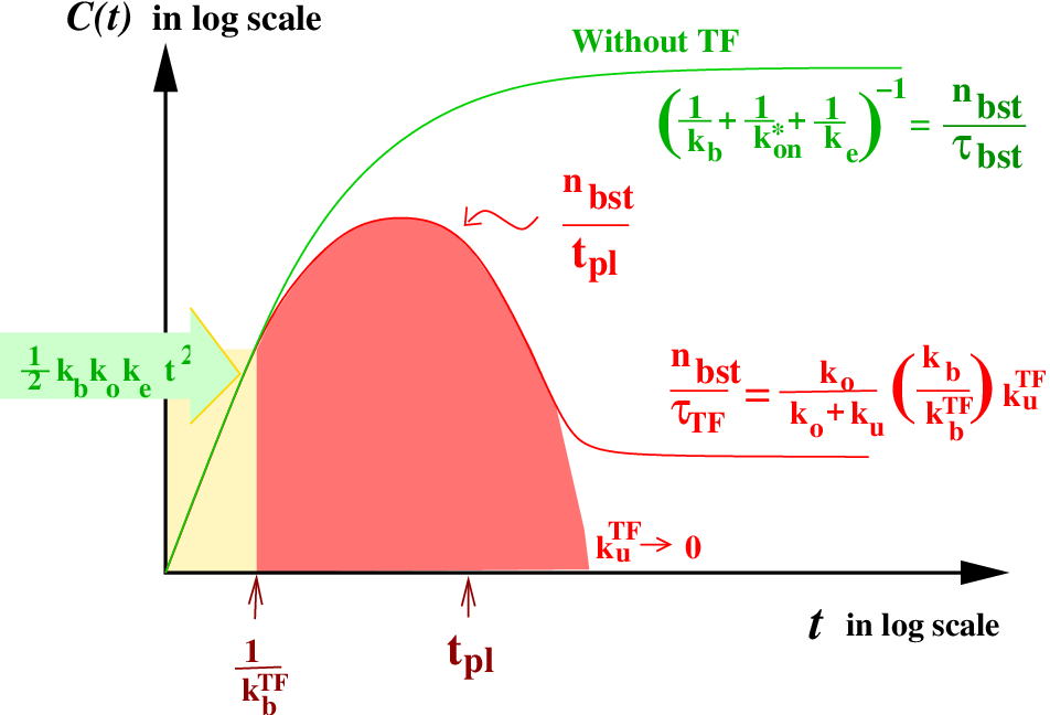
With all these results, Fig.7 summarizes the behavior of time dependent activity $C(t)$ for the promoter with fast initial binding/unbinding under the strong but slow TF repression:

(k_{u},\,k_{b})\,\mathrel{\hbox to0.0pt{\lower 4.0pt\hbox{\hskip 1.0pt$\sim$}\hss}\raise 1.0pt\hbox{$>$}}(k_{b}^{\rm TF},\,k_{o},\,k_{e})\gg k_{u}^{\rm TF},

(31)

where we have a typical bursting of transcriptions with

n_{\rm bst}\mathrel{\hbox to0.0pt{\lower 4.0pt\hbox{\hskip 1.0pt$\sim$}\hss}\raise 1.0pt\hbox{$>$}}1,\quad\tau_{\rm TF}\gg t_{\rm pl}\approx\tau_{\rm bst}.

(32)

After the clarification of the promoter and operator sites, the activity increases initially as

C(t)\approx{1\over 2}k_{b}k_{o}k_{e}t^{2},\qquad\mbox{for }t\mathrel{\hbox to0.0pt{\lower 4.0pt\hbox{\hskip 1.0pt$\sim$}\hss}\raise 1.0pt\hbox{$<$}}{1\over k_{b}^{\rm TF}}

(33)

until TF starts binding.

Then, it reaches the (maximum) plateau value:

C_{\rm max}\approx{n_{\rm bst}\over t_{\rm pl}}={n_{\rm bst}\over n_{\rm bst}+1}\cdot{1\over 1/k_{o}+1/k_{e}}\quad\mbox{for }t\mathrel{\hbox to0.0pt{\lower 4.0pt\hbox{\hskip 1.0pt$\sim$}\hss}\raise 1.0pt\hbox{$<$}}t_{\rm pl}.

(34)

Finally, $C(t)$ diminishes down to the long time averaged steady value with TF,

\Omega_{\rm TF}={n_{\rm bst}\over\tau_{\rm bst}+\tau_{\rm TF}}\approx{n_{\rm bst}\over\tau_{\rm TF}}

(35)

From eqs.(34) and (35), the enhancement factor $f_{\rm enh}$ that the promoter can be activated after the clearance of the site is given by

f_{\rm enh}\equiv{C_{\rm max}\over\Omega_{\rm TF}}\approx{\tau_{\rm bst}+\tau_{\rm TF}\over t_{\rm pl}}\approx{\tau_{\rm TF}\over t_{\rm pl}}

(36)

This expression formalizes our original discussion that one obtain large relative peak activity when TF repression is strong, $(\tau_{\rm bst},\,t_{\rm pl})\ll\tau_{\rm TF}$ , but slow $k_{b}^{\rm TF}\ll k_{b}$ , namely, $n_{\rm bst}\gg 1$ . The promoters with shorter “internal time” $1/k_{o}+1/k_{e}$ have larger relative peak activity, and therefore they will be more prone to de-repression by TI.

Interfering with Regulated Promoter Activity

We now consider the interfering promoters pS and pA where pA is relatively strong in comparison with pS, and pS is strongly repressed by a slow TF. In this case, the average activity $\Omega_{\rm TI}$ is given by eq.(10), using the time-dependent activity $C(t)$ without TI and the elongation interval distribution $p_{A}(\tau)$ of pA.

In the following, we ignore the occlusion time $\tau_{\rm occ}$ by RNAP from pA; This should not be bad for the promoter whose activity is of order or less than 0.1 s^-1, but may not be so good for a more active promoter. For $p_{A}(\tau)$ , we will use the exponential distribution (11), which corresponds to the single step Poissonian promoter pA.

The expression for $\Omega_{\rm TI}$ of (10) basically gives the average of $C(t)$ over the typical time scale of pA, which is $\Omega_{A}^{-1}$ . Therefore, if you look at $\Omega_{\rm TF}$ as a function of $\Omega_{A}$ , then $\Omega_{\rm TI}$ would show a maximum around $\Omega_{A}\sim 1/t_{\rm max}$ in the case that $C(t)$ has a maximum around $t\approx t_{\rm max}$ .

Two step model:

we can obtain the explicit expression for $\Omega_{\rm TI}$ , which can be approximated as

\Omega_{\rm TI}\approx{n_{\rm bst}\over t_{\rm pl}+\Omega_{A}^{-1}}\times{k_{b}^{\rm TF}+k_{\rm on}\over k_{b}^{\rm TF}+k_{\rm on}+\Omega_{A}}

(37)

for $\Omega_{A}\gg k_{u}^{\rm TF}$ in the regime $k_{b}^{\rm TF}\gg k_{e}\gg k_{u}^{\rm TF}$ . Here, $n_{\rm bst}$ is the number of transcriptions in a burst defined in eq.(19), and $t_{\rm pl}$ is the plateau time (23). This expresses the activity of the de-repressed two-step promoter in terms of the product of two factors; the first factor corresponds to the averaged activity for the bursting whose interval is given by $t_{\rm pl}+\Omega_{A}^{-1}$ . This factor represents the de-repression by the interference through removal of TF by RNAP from pA before it dissociates by itself. The second factor represents the suppression by removing the open complex, i.e. sitting duck interference.

The expression (37) shows a maximum

\Omega_{\rm TI,max}\approx{n_{\rm bst}\over t_{\rm pl}}\quad\mbox{at }\Omega_{A}\approx\sqrt{k_{b}^{\rm TF}+k_{\rm on}\over t_{\rm pl}}

(38)

which corresponds to eq.(22). The promoter activity is actually increased by the transcription interference. The enhancement factor, or the ratio $\Omega_{\rm TI,max}/\Omega_{\rm TF}$ , is the same as in eq.(36).

Three step model:

We cannot write down a compact expression, but Fig.8 shows $\Omega_{\rm TI}$ vs. $\Omega_{A}$ (lower panels) along with the corresponding $C(t)$ (upper panels) for the three step model with different values of parameters. One can see the correspondence between the upper and lower panels: The activity as function of $\Omega_{A}$ approximately resembles the activity profiles a time $t\sim 1/\Omega_{A}$ plotted in corresponding upper panels. Notice also that the potential activation by a convergent promoter is largest for large $k_{o}$ and $k_{e}$ , as expected from eq.(36). Finally, the relative effect of de-repression can be very large, in the case of very slow dissociation rate for the transcription factor.

Summary and Discussions

We have presented a mathematical framework that expresses the dynamics of a promoter in the Hawley-McClure model. The formalism opens for discussion on the promoter activity with transcription factors (TF) and transcriptional interference (TI) by an interfering promoter, and allows us to deal with the interplay among these elements.

In our formalism, the activity of a single promoter is characterized by the correlation function $C(t)$ , which represents the averaged time dependent activity after the transcription initiation at $t=0$ . Any modifications to the activity of the single promoter, such as that by TF, are taken into account through the correlation function $C(t)$ . On the other hand, the effects from an interfering promoter punctuates the promoter/operator activity with the time scale of transcription initiation from the interfering promoter. This is represented by the expression (10).

We have studied the effects of a repressive TF on the promoter activity. The general expressions for the promoter activity can be put in the form that is associated with the transcription burst, namely, a burst of $n_{\rm bst}$ transcriptions during the bursting time $\tau_{\rm bst}$ followed by a quiescent period of the length $\tau_{\rm TF}$ . This is actually what happens in the case of a strongly repressed promoter by a slow binding TF. It should be noted that the “equilibrium formula” (14) for the promoter activity repressed by TF is not valid unless the time scales of internal processes are negligible compared with binding/unbinding times of RNAP, because a TF competes with RNAP for binding to DNA.

Under the transcription interference (TI) considered in the present work, an interfering RNAP simply clears both the promoter and operator sites. If the promoter is strongly repressed by a TF, such interference is most likely to relieve the promoter out of repression, and interrupts the quiescent period to shorten to $1/\Omega_{A}$ when $\Omega_{A}>k_{u}^{TF}$ .

Experimental Observations

Let us discuss experimental relevance of our theoretical results for transcription burst and its modification by transcription interference.

Transcription Bursts:

Experimentally, bunched promoter activities have been seen in several eucaryotic systems involving TF’s [26, 27], and they have been interpreted to occur in response to transformation in heterochromatin states, or as a result of a promoter approaching transcription factories [28]. For procaryotes, bunched activities have only been observed for the promoter $P_{\rm lac/ara}$ under the fully induced condition[29], and has been interpreted without TF[30].

On the other hand, transcription bursts induced by activators have been examined in models and experiments on the yeast GAL1-promoter [31], considering transcription activation by the TATA-binding protein. The operator position has been also shown to influence “bunchiness” of a promoter[32].

To the best of our knowledge, transcription bursts due to repressor as are analyzed in the present paper have not been observed yet experimentally.

Transcription Interference:

We have, at present, no direct experimental evidences for the possibility of de-repression by transcriptional interference(TI). Its biological relevance, however, could be widespread in phage and E. coli; Convergent promoters is a common regulatory motif for all temperate phages that has a CII like protein, and about 100 examples of convergent promoters have been also found in E. coli [14].

To show how TI with de-repression could help us to understand a biological system, let us discuss the hyp-mutant of lambda; This system is intriguing because of its high production of Cro in the lysogeny and its enhanced immunity against infection of other lambdas[33, 34]. Its DNA configuration resembles that in Fig.1(b) and the parameters in Fig.8 are matched to this system. Therefore, the maximal repression case there corresponds to the case of the promoter PR in lambda repressed by the factor of about 500 due to CI [35, 36, 37]. The strength of hyp-PRE is not known, but Fig.8 suggests that PR in lysogen could be de-repressed by the factor 10 $\sim$ 30 due to TI from hyp-PRE, provided that open complex formation is fast and that CI binds to OR relatively slowly. This could explain, at least, a part of the large amount of Cro found in the lysogeny of the hyp-mutant.

Another example is the $O_{R3}O_{R2}O_{R3}$ mutant, which has been also found to show stable lysogens[38], even though it is expected to be producing Cro 10 $\sim$ 30 times more than a normal lambda[4], as in the case of the hyp-mutant. Such similarity, i.e. the stable lysogens under the high production of Cro, between the $O_{R3}O_{R2}O_{R3}$ and the hyp-mutant leads us to speculate that the remarkable robustness of the lysogens[39] of these phages should be rooted in the same unknown mechanism.

Experimental Proposal

Burst activity should be most directly monitored by a real time observation, but also can be examined quantitatively from the number distribution of mRNA in a cell. This may be obtained if one can take snapshots of an assembly of cells from which the number of mRNA contained in each cell can be counted. The reaction rate constants for RNAP and TF should be able to be estimated from the mRNA distribution.

For example, from the distribution one can calculate the Fano factor $\nu$ , which is the ratio of the variance to the average

\nu\equiv{\left<(n-\left<n\right>)^{2}\right>\over\left<n\right>}

(39)

with $n$ being the number of mRNA in a cell. This Fano factor can be directly compared with our estimate of the number of transcriptions in a burst $n_{\rm bst}$ ; In the bursting situation with $n_{\rm bst}\gg 1$ , the Fano factor should be given by $n_{\rm bst}$ if the quiescent periods follow Poissonian process and are much longer than the bursting periods:

\nu\sim n_{\rm bst}={k_{b}\over k_{b}^{\rm TF}}\cdot{k_{o}\over k_{o}+k_{u}}\qquad\mbox{for }\tau_{\rm bst}\ll\tau_{\rm TF},

(40)

but is smaller than that if the burstings are not separated well enough:

\nu<n_{\rm bst}\qquad\mbox{for }\tau_{\rm bst}\mathrel{\hbox to0.0pt{\lower 4.0pt\hbox{\hskip 1.0pt$\sim$}\hss}\raise 1.0pt\hbox{$<$}}\tau_{\rm TF}.

(41)

In the case $n_{\rm bst}\ll 1$ , we would have $\nu\sim 1$ because each elongation initiation follows the Poissonian process. The full information of the distribution allows us more detailed comparison with our analysis.

Another experiment we can propose is to construct DNA with a promoter exposed to a library of interfering promoters with varying strength $\Omega_{A}$ , preferably in a parallel configuration to avoid RNAP collisions. Suppose the promoter is highly repressed by TF with unknown parameters. By examining how the promoter is de-repressed by the interfering promoters, the off-rate $k_{u}^{TF}$ of TF can be estimated as the lower limit of $\Omega_{A}$ that de-represses the promoter.

Simplifications in the Present Treatment

Before concluding, let us discuss some of the effects we have ignored in the present treatment.

Roadblock:

In our analysis of TI, we have assumed that RNAP always displaces TF without roadblock effect, but it is known that some TF’s are roadblocks to RNAP. Roadblocks are most commonly reported in in-vitro experiments [40, 41, 42], whereas presence of elongation factors often allow RNAP to pass the roadblock in in-vivo situations [42, 43]. Reports on in-vivo roadblocks is at present limited to the transcription factor LacI and the restriction enzyme EcoRI [44]. It has been reported that some roadblocks may be translocated, being pushed by two or more RNAP’s[44]. If two consecutive RNAP’s are required to dislocate a TF, the activity of interfering promoter $\Omega_{A}$ in eq.(37) should be replaced by the effective activity, which is half of the original activity, $\Omega_{A}/2$ . This reduction factor 1/2 should be further reduced in the case where a blocked RNAP may fall off before the second one arrives to give a push.

Another possibility that RNAP does not remove TF is that RNAP just passes TF without displacing it; The repressor would simply not leave the vicinity of the operator, and thus maintains its function until it falls off by itself. This kind of situation has been actually observed when an RNAP reads through a nucleosome, displacing only parts of the histone complex[45, 46]. For some TF, one could imagine mixed situations, where TF is displaced but remains in physical proximity during the RNAP passage.

TF’s such as CI in phage 186 [11] and CI in $\lambda$ on OR [37] do not act as roadblocks but are removed, which, we presume, are more common situations.

Time difference for the promoter and the operator:

The interfering RNAP’s clear/occlude the promoter pS first and then the operator in the convergent configuration, and the other way around in the parallel configuration. The time difference of the effects for the two sites depends on the distance between the two sites. If the binding times of TF or RNAP are comparable or shorter than this time difference, we have to take this into account, which makes the situation favorable to the promoter(operator) in the convergent(parallel) configuration.

RNAP collision:

The RNAP from pS may be removed, even after it starts elongating, by colliding with the RNAP from pA. This effect is profound particularly when the distance between pS and pA is large. It has been found that the collision effect becomes substantial for convergent promoters with the pS-pA distance being of the order of $v/(2\Omega_{A})$ , where $v$ ( $\sim 50$ bp/sec) is the transcription elongation speed[14]. For the parallel configuration of promoters, the collision effect does not exist.

Occlusion time:

The occlusion time $\tau_{\rm occ}$ , the time that the promoter pS is occluded by passing the RNAP from pA, was neglected. This has been also considered in [14] and found that pS is influenced substantially by occlusion only when the activity of pA is stronger than 0.1 s^-1.

Mutual interference:

In the convergent configuration of promoters, not only pA interferes with pS, but also pS interferes with pA. Such mutual interference effects are likely to be important in switching mechanisms between equally strong convergent promoters, such as the convergent promoters PR and PRE of lambda phage in the early stages of infection. Full analytical treatment on the mutual interference is not easy in general case, but stochastic simulations [14] and the four-world approximation analysis [15] have been performed. In the present analysis, we consider the highly repressed promoter pS, thus the interference of pS on pA should be negligible. In the case of the parallel configuration, this effect does not exist.

Acknowledgment: We very much like to thank Ian Dodd, Alexandra Ahlgren-Berg, and Adam Palmer for discussions on transcription interference, and Harvey Eisen for suggesting that transcribing RNAP from the hyp-PRE promoter may reduce CI repression of PR in the hyp-mutant of phage lambda. We thank for financial support from the Danish National Research Foundation through the Center for Models of Life.

Appendix: Promoter Activity in Michaelis-Menten Form

Since the process of transcription initiation can be regarded as an enzyme reaction, our results for the averaged promoter activity in the three step model can be put in the form of Michaelis-Menten kinetics.

Let us start by the bare activity without TF. The binding rate $k_{b}$ of RNAP should be proportional to the density of RNAP,

k_{b}\equiv[{\rm RNAP}]\kappa_{b}

(42)

with a reaction constant $\kappa_{b}$ . Then, the bare activity (4) can be written as

\Omega_{0}={[{\rm RNAP}]/K^{*}_{\rm RNAP}\over 1+[{\rm RNAP}]/K^{*}_{\rm RNAP}}\,\Omega_{0}^{\rm max}

(43)

with the maximum activity

\Omega_{0}^{\rm max}\equiv{k_{o}k_{e}\over k_{o}+k_{e}},

(44)

and the effective dissociation constant for RNAP

K^{*}_{\rm RNAP}\equiv\left(1+{k_{u}\over k_{o}}\right){\Omega_{0}^{\rm max}\over\kappa_{b}}.

(45)

TF has been introduced as a competitive inhibitor in our model. Its binding rate can be expressed as

k_{b}^{\rm TF}\equiv[{\rm TF}]\kappa_{b}^{\rm TF},

(46)

with the TF density [TF] and the reaction constant $\kappa_{b}^{\rm TF}$ , then the dissociation constant for TF is given by

K_{\rm TF}\equiv{k_{u}^{\rm TF}\over\kappa_{b}^{\rm TF}}.

(47)

With these parameters, the expression (25) for the averaged activity with TF is written as

\Omega_{\rm TF}={\displaystyle{[{\rm RNAP}]/K^{*}_{\rm RNAP}}\over\displaystyle 1+{[{\rm TF}]/K_{\rm TF}}+{[{\rm RNAP}]/K^{*}_{\rm RNAP}}}\,\Omega_{0}^{\rm max},

(48)

which is in the standard form of Michaelis-Menten kinetics with a competitive inhibitor.

References

[1] Ptashne, M., and A. Gann, 1997. Transcriptional activation by recruitment. Nature 386:569–577.
[2] Roy, S., S. Garges, and S. Adhya, 1998. Activation and Repression of Transcription by Differential Contact: Two Sides of a Coin. J. Biol. Chem. 273:14059–14062.
[3] Shea, M. A., and G. K. Ackers, 1985. The OR control system of bacteriophage lambda. A physical-chemical model for gene regulation. J. Mol. Biol. 181:211–230.
[4] Sneppen, K., and G. Zocchi, 2005. Physics in Molecular Biology, Cambridge university press, 195–196.
[5] Winter, R. B., O. G. Berg, and P. H. von Hippel, 1981. Diffusion-Driven Mechanisms of Protein Translocation on Nucleic Acids. 3. The Escherichia coli lac Repressor-Operator Interaction: Kinetic Measurements and Conclusions. Biochemistry 20:6961–6977.
[6] Elf, J., G.-W. Li, and S. Xie, 2007. Probing Transcription Factor Dynamics at the Single Molecule Level in a Living Cell. Science 316:1191–1194.
[7] Liang, S.-T., M. Bipatnath1, Y.-C. Xu1, S.-L. Chen, P. Dennis, M. Ehrenberg, and H. Bremer, 1999. Activities of consitutive promoters in Escherichia coli. J. Mol. Biol. 292:19–37.
[8] Ward, D. F., and N. E. Murra, 1979. Convergent transcription in bacteriophage lambda: interference with gene expression. J. Mol. Biol. 133:249–266.
[9] Adhya, S., and M. Gottesman, 1982. Promoter occlusion: transcription through a promoter may inhibit its activity. Cell 29:939–944.
[10] Menendez, M., A. Kolb, and H. Buc, 1987. A NEW TARGET FOR CRP ACTION AT THE MALT PROMOTER. EMBO J. 6:4227–4234.
[11] Callen, B. P., K. E. Shearwin, and J. B. Egan, 2004. Transcriptional interference between convergent promoters caused by elongation over the promoter. Mol. Cel. 14:647–656.
[12] Greger, I. H., A. Aranda, and N. Proudfoot, 2000. Balancing transcriptional interference and initiation on the GAL7 promoter of Saccharomyces cerevisiae. Proc. Natl. Acad. Sci. USA 97:8415–8420.
[13] Prescott, E. M., and N. J. Proudfoo, 2002. Transcriptional collision between convergent genes in budding yeast. Proc. Natl. Acad. Sci. USA 99:8796–8801.
[14] Sneppen, K., I. B. Dodd, K. E. Shearwin, A. C. Palmer, R. A. Schubert, B. P. Callen, and J. B. Egan, 2005. A mathematical model for transcriptional interference by RNA polymerase traffic in Escherichia coli. J. Mol. Biol. 346:399–409.
[15] Dodd, I. B., K. E. Shearwin, and K. Sneppen, 2007. Modeling transcriptional interference and DNA looping in gene regulation. J. Mol. Biol. 369:1200–1213.
[16] Hawley, D., and W. McClure, 1982. Mechanism of activation of transcription initiation from the lambda PRM promoter. J. Mol. Biol. 57:493–525.
[17] Buc, H., and W. R. McClure, 1985. Kinetics of open complex formation between Escherichi coli RNA polymerase and the lac UV5 promoter. Evidence for a sequential mechanism involving three steps. Biochemistry 24:2712–2723.
[18] Record Jr, M. T., W. S. Reznikoff, M. L. Craig, K. L. McQuade, and P. J. Schlax, 1996. Escherichia coli RNA polymerase(E $\sigma$ 70) promoters, and the kinetics of the steps of transcription initiation. In F. C. Neidhardt, R. C. III, J. L. Ingraham, E. C. C. Lin, K. R. Low, B. Magasanik, W. S. Reznikoff, M. Riley, M. Schaechter, and H. E. Umbarger, editors, Escherichia coli and Salmonell. typhimurium. American Society for Microbiology, Washington DC, 792–820.
[19] Hsu, L. M., 2002. Promoter clearance and escape in prokaryotes. Biochimica et Biophysica Acta 1577:191–207.
[20] Knaus, R., and H. Bujard, 1988. PL of coliphage lambda: an alternate solution for an efficient promoter. EMB J. 7:2919–2923.
[21] Carpousis, A. J., J. E. Stefano, and J. D. Gralla, 1982. 5’ nucleotide heterogeneity and altered initiation of transcription at mutant lac promoters. J. Mol. Biol. 157:619–633.
[22] Darzacq, X., Y. Shav-Tal1, V. de Turris1, Y. Brody, S. M. Shenoy, R. D. Phair, and R. H. Singer, 2007. In vivo dynamics of RNA polymerase II transcription. Nature Structural and Molecular Biology 14:796–806.
[23] Lanzer, M., and H. Bujard, 1988. Promoters largely determine the efficiency of repressor action. Proc. Natl. Acad. Sci. USA 85:8973–8977.
[24] A java applet for the promoter model with a transcription factor is available at http://cmol.nbi.dk/models/dynamtrans/
dynamtrans.html.
[25] $\tau_{occ}=(r+\ell)/v$ is the time needed to for a RNAP from pA totranscribe acros the pS promoter (length $r+\ell\sim 105bp$ and speed $v$ estimated to be 50bp/sec [14]).
[26] Chubb, J. R., T. Trcek, S. M. Shenoy, and R. H. Singer, 2006. Transcriptional pulsing of a developmental gene. Curr. Biol. 16:R371–3.
[27] Raj, A., C. Peskin, D. Tranchina, D.Y.Vargas, and S. Tyagi, 2006. Stochastic mRNA Synthesis in Mammalian Cell. Plos Biol. 1707–1719.
[28] Cook, P. R., 1999. The organization of replication and transcription. Science 284:1790–1795.
[29] Golding, I., J. Paulsson, S. M. Zawilski, and E. Cox, 2005. Real time kinetics of gene activity in individual bacteria. Cell 123:1025–1036.
[30] Mitarai, N., I. B. Dodd, M. T. Crooks, and K. Sneppen, 2008. The generation of promoter-mediated transcriptional noise in bacteria. PloS Comput. Biol. Accepted for publication.
[31] Blake, W. J., G. Balázsi, M. A. Kohanski, F. J. Isaacs, K. F. Murphy, Y. Kuang, C. R. Cantor, D. R. Walt, and J. J. Collins, 2006. Phenotypic Consequences of Promoter-Mediated Transcriptional Noise. Mol. Cell 24:853–865.
[32] Murphy, K. F., G. Balázsi, and J. J. Collins, 2007. Combinatorial promoter design for engineering noisy gene expression. Proc. Natl. Acad. Sci. USA 104:12726–12731.
[33] Eisen, H., P. Barrand, W. Spiegelman, L. F. Reichardt, S. Heineman, and C. Georgopoulos, 1982. Mutants in the Y-Region of Bacteriophage $\lambda$ constitutive for repressor synthesis: Their isolation and the characterization of the Hyp phenotype. Gene 20:71–81.
[34] Georgopoulos, C., N. McKittric, G. Herrick, and H. Eisen, 1982. An IS4 transposition causes a 13-bp duplication of Phage-lambda DNA and results in the constitutive expression of the CI and Cro Gene-products. Gene 20:83–90.
[35] Révet, B., B. von Wilcken-Bergmann, H. Bessert, A. Barker, and B. Muller-Hil, 1999. Four dimers of lambda repressor bound to two suitably spaced pairs of lambda operators form octamers and DNA loops over large distances. Curr. Biol. 9:151–154.
[36] Dodd, I. B., K. E. Shearwin, A. J. Perkins, T. Burr, A. Hochschild, and J. B. Egan, 2004. Cooperativity in long-range gene regulation by the $\lambda$ CI repressor. Genes and Development 18:344–354.
[37] Ahlgen-Berg, A., and I. Dodd. private communication.
[38] Little, J. W., D. P. Shepley, and D. W. Wert, 1999. Robustness of a gene regulatory circuit. EMBO Journal 18:4299–4307.
[39] Aurell, E., S. Brown, J. Johansen, and K. Sneppen, 2002. Stability puzzles in phage $\lambda$ . Phys. Rev. E 65:51914.
[40] Pavco, P., and D. Steege, 1990. Elongation by Escherichia coli RNA polymerase is blocked in vitro by a site-specific DNA binding protein. J. Biol. Chem. 265:9960–9969.
[41] Iban, M. G., and D. S. Luse, 1991. Transcription on nucleosomal templates by RNA polymerase II in vitro: inhibition of elongation with enhancement of sequence-specific pausing. Genes Dev. 5:683–696.
[42] Reines, D., and J. Mote, 1993. Elongation factor SII-dependent transcription by RNA polymerase II through a sequence-specific DNA-binding protein. Proc. Natl. Acad. Sci. USA 90:1917–1921.
[43] Toulmé, F., C. Mosrin-Huaman, J. Sparkowski, A. Das, M. Leng, and A. Rahmouni, 2000. GreA and GreB proteins revive backtracked RNA polymerase in vivo by promoting transcript trimming. EMBO J. 19:6853–6859.
[44] Epshtein, V., F. Toulmé, A. Rahmouni, S. Borukhov, and E. Nudler, 2003. Transcription through the roadblocks: the role of RNA polymerase cooperation. EMBO J. 22:4719–4727.
[45] Kireeva, M. L., W. Walter, V. Tchernajenko, V. Bondarenko, M. Kashlev, and V. M. Studitsky, 2002. Nucleosome Remodeling Induced by RNA Polymerase II: Loss of the H2A/H2B Dimer during Transcription. Molec. Cell 9:541–552.
[46] Walter, W., M. L. Kireeva, V. M. Studitsky, and M. Kashlev, 2003. Bacterial Polymerase and Yeast Polymerase II Use Similar Mechanisms for Transcription through Nucleosomes. J. Biol. Chem. 278:36148–36156.

Supplement for
“Dynamical Analysis on Gene Activity
in the Presence of Repressors and an Interfering Promoter”

Hiizu Nakanishi ^1,2, Namiko Mitarai ², and Kim Sneppen ¹

¹ Niels Bohr Institute , Blegdamsvej 17, Dk 2100, Copenhagen, Denmark
² Department of Physics, Kyushu University 33, Fukuoka 812-8582, Japan

(August 24, 2026)

Appendix I. Elongation Initiation Interval and Correlation

Let $C(t)$ be the time-dependent activity after the clearance of both the promoter and the operator. Then it can also be regarded as a correlation function of the transcription initiation, and it is related to the initiation interval distribution $p(\tau)$ as

$\displaystyle C(t)=p(t)+\int_{0}^{\infty}d\tau_{1}\int_{0}^{\infty}d\tau_{2}\,\delta(t-\tau_{1}-\tau_{2})\,p(\tau_{1})p(\tau_{2})$		(1)
	$\displaystyle\quad+\int_{0}^{\infty}d\tau_{1}\int_{0}^{\infty}d\tau_{2}\int_{0}^{\infty}d\tau_{3}\,\delta(t-\tau_{1}-\tau_{2}-\tau_{3})\,p(\tau_{1})p(\tau_{2})p(\tau_{3})$
	$\displaystyle\qquad+\cdots.$

Since each term in the right hand side is a convolution of $p(\tau)$ , the Laplace transformation

\tilde{C}(s)\equiv\int_{0}^{\infty}C(t)e^{-st}dt

(2)

can be obtained easily as a sum of geometrical series;

\tilde{C}(s)=\sum_{n=1}^{\infty}\tilde{p}(s)^{n}={\tilde{p}(s)\over 1-\tilde{p}(s)}

(3)

with $\tilde{p}(s)$ being the Laplace transform of $p(\tau)$ .

Appendix II. Bare Promoters

In this section, the explicit expressions for $p(\tau)$ and $C(t)$ for a bare promoter of each model are derived within the approximation that the self-occlusion effect is ignored.

A. Single step model

For the single step model, the elongation initiation is a simple Poissonian process with the rate $\Omega_{0}$ , thus we have

p(\tau)=\Omega_{0}e^{-\Omega_{0}\tau},\qquad\tilde{p}(s)={\Omega_{0}\over s+\Omega_{0}},

(4)

and

\tilde{C}(s)={\Omega_{0}\over s},\qquad C(t)=\Omega_{0}.

(5)

B. Two step model

In the two step model, each elongation interval consists of an off-state period and an on-state period, whose length distributions, $p_{\rm off}(\tau_{\rm off})$ and $p_{\rm on}(\tau_{\rm on})$ , are Poissonian given by

p_{\rm off}(\tau_{\rm off})=k_{\rm on}e^{-k_{\rm on}\tau_{\rm off}},\quad\mbox{and}\quad p_{\rm on}(\tau_{\rm on})=k_{e}e^{-k_{e}\tau_{\rm on}},

(6)

respectively. Since the elongation interval is the sum of the off-period length and the on-period length, the elongation interval distribution $p(\tau)$ for the two step model is given by

p(\tau)=\int_{0}^{\infty}d\tau_{\rm off}\int_{0}^{\infty}d\tau_{\rm on}\,\delta(\tau-\tau_{\rm off}-\tau_{\rm on})p_{\rm off}(\tau_{\rm off})p_{\rm on}(\tau_{\rm on}).

(7)

Again, the right hand side is a convolution of $p_{\rm off}(\tau_{\rm off})$ and $p_{\rm on}(\tau_{\rm on})$ , thus in the Laplace transform, we have

\tilde{p}(s)=\tilde{p}_{\rm off}(s)\,\tilde{p}_{\rm on}(s)={k_{\rm on}k_{e}\over(s+k_{\rm on})(s+k_{e})},

(8)

which gives

p(\tau)=\left\{\begin{array}[]{ll}\displaystyle k_{\rm on}k_{e}\,{e^{-k_{e}\tau}-e^{-k_{\rm on}\tau}\over k_{\rm on}-k_{e}}&\mbox{for }k_{\rm on}\neq k_{e}\\ \displaystyle k_{e}^{2}\,\tau\,e^{-k_{e}\tau}&\mbox{for }k_{\rm on}=k_{e}\end{array}\right..

(9)

Then, the correlation function is given by

\tilde{C}(s)={k_{\rm on}k_{e}\over s(s+k_{\rm on}+k_{e})},\quad C(t)=\Omega_{0}\left(1-e^{-(k_{\rm on}+k_{e})t}\right)

(10)

with $\Omega_{0}$ being the bare activity for the two step model:

\Omega_{0}={k_{\rm on}k_{e}\over k_{\rm on}+k_{e}}={1\over\tau_{\rm on}+\tau_{e}};\qquad\tau_{\rm on}\equiv{1\over k_{\rm on}},\quad\tau_{e}\equiv{1\over k_{e}}.

(11)

Note that the last expression simply represents that the average interval between elongation $1/\Omega_{0}$ is the sum of the average waiting time to become the on-state $\tau_{\rm on}$ and the time for the elongation $\tau_{e}$ .

C. Three step model

In the three step model, the initial transition between the off-state and the closed complex state is reversible, which means that the closed state goes either back to the off-state or forward to the open complex state with the branching ratios $k_{u}$ and $k_{o}$ , or with the probabilities

p\equiv{k_{u}\over k_{u}+k_{o}},\quad\mbox{and}\quad q\equiv{k_{o}\over k_{u}+k_{o}}=1-p,

(12)

respectively. Therefore, the promoter may get into the closed state many times before an RNAP starts elongation. Let $n$ be the number of times that the promoter gets in the closed state before elongation, then the sequence of states and their probabilities are

\begin{array}[]{ccc}n&\mbox{state sequence}&\mbox{probability}\\ \hline\cr 1&\mbox{(off - closed) $\bullet$ open - elong}&q\\ 2&\quad\mbox{(off - closed) $\circ$ (off - closed) $\bullet$ open - elong}&p\,q\\ &\cdot\cdot\cdot&\\ n&\mbox{(off - closed $\circ$)${}^{n-1}$(off - closed) $\bullet$ open - elong}&p^{n-1}q\\ &\cdot\cdot\cdot&\\ \end{array},

(13)

where $\circ$ and $\bullet$ represent the branching probabilities $p$ and $q$ , respectively.

Let $p_{n}(\tau)$ be the elongation interval distribution for the interval during which the promoter goes through the closed state $n$ times, then it is given by a convolution of the life time distribution of the off-state $p_{\rm off}(\tau)$ , the closed state $p_{\rm cl}(\tau)$ , and the open state $p_{\rm op}(\tau)$ ; For example, $p_{1}(\tau)$ is given by

p_{1}(\tau)=\int_{0}^{\infty}d\tau_{\rm off}\int_{0}^{\infty}d\tau_{\rm cl}\int_{0}^{\infty}d\tau_{\rm op}\,\delta(\tau-\tau_{\rm off}-\tau_{\rm cl}-\tau_{\rm op})p_{\rm off}(\tau_{\rm off})p_{\rm cl}(\tau_{\rm cl})p_{\rm op}(\tau_{\rm op}).

(14)

In the same way, the Laplace transform of $p_{n}(\tau)$ for general $n$ is given by

\tilde{p}_{n}(s)=\Bigl(\tilde{p}_{\rm off}(s)\tilde{p}_{\rm cl}(s)\Bigr)^{n}\tilde{p}_{\rm op}(s)

(15)

with

\tilde{p}_{\rm off}(s)={k_{b}\over s+k_{b}},\quad\tilde{p}_{\rm op}(s)={k_{u}+k_{o}\over s+k_{u}+k_{o}},\quad\tilde{p}_{\rm cl}(s)={k_{e}\over s+k_{e}}.

(16)

The elongation interval distribution $p(\tau)$ is the average over $p_{n}(\tau)$ with the probability given by (13), and can be calculated as follows;

\tilde{p}(s)=\sum_{n=1}^{\infty}\tilde{p}_{n}(s)\,p^{n-1}q\quad={\tilde{p}_{\rm off}(s)\tilde{p}_{\rm cl}(s)\over 1-\tilde{p}_{\rm off}(s)\tilde{p}_{\rm cl}(s)p}\,\,\tilde{p}_{\rm op}(s)\,q\quad={k_{b}k_{o}k_{e}\over(s+k_{+})(s+k_{-})(s+k_{e})}

(17)

with

k_{\pm}\equiv{1\over 2}\Bigl[(k_{b}+k_{u}+k_{o})\pm\sqrt{(k_{b}+k_{u}+k_{o})^{2}-4k_{b}k_{o}}\Bigr],

(18)

from which we obtain

p(\tau)={k_{b}k_{o}k_{e}\over(k_{e}-k_{+})(k_{e}-k_{-})}e^{-k_{e}\tau}+{k_{b}k_{o}k_{e}\over\sqrt{(k_{b}+k_{o}+k_{e})^{2}-4k_{b}k_{o}}}\left[{e^{-k_{-}\tau}\over k_{e}-k_{-}}-{e^{-k_{+}\tau}\over k_{e}-k_{+}}\right].

(19)

From eqs.(3) and (17), we have

\tilde{C}(s)={k_{b}k_{o}k_{e}\over s(s+k_{+}^{C})(s+k_{-}^{C})};\quad k_{\pm}^{C}\equiv{1\over 2}\left[(k_{b}+k_{u}+k_{o}+k_{e})\pm\sqrt{(k_{b}+k_{u}+k_{o}-k_{e})^{2}-4k_{b}k_{o}}\right],

(20)

which leads to

C(t)=\Omega_{0}\left[1-{k_{+}^{C}e^{-k_{-}^{C}t}-k_{-}^{C}e^{-k_{+}^{C}t}\over k_{+}^{C}-k_{-}^{C}}\right]

(21)

where $\Omega_{0}$ is the bare activity for the three step model:

\Omega_{0}={k_{b}k_{o}k_{e}\over k_{+}^{C}k_{-}^{C}}\quad={1\over\tau_{b}+\tau_{o}^{*}+\tau_{e}};\qquad\tau_{b}\equiv{1\over k_{b}},\quad\tau_{o}^{*}\equiv{1\over k_{\rm on}^{*}}={1\over k_{o}}+{k_{u}\over k_{o}}\cdot{1\over k_{b}},\quad\tau_{e}\equiv{1\over k_{e}}.

(22)

The average interval between elongations, $1/\Omega_{0}$ , are the sum of the three times: (1) $\tau_{b}$ , the time for RNAP to bind and form the closed complex for the first time, (2) $\tau_{o}^{*}$ , the time for RNAP to form the open complex after the first binding, and (3) $\tau_{e}$ , the time to start elongation. Note that the validity of this expression is not limited to the case within the two step approximation, where $k_{\rm on}^{*}$ can be interpreted as the effective on-rate.

The time $\tau_{o}^{*}$ consists of two parts: (i) $1/k_{o}$ , the time to go forward to the open state, and (ii) the re-binding time $1/k_{b}$ after unbinding multiplied by the average number of unbindings $k_{u}/k_{o}$ . Mathematical derivation of this expression is given in the appendix. We will encounter similar expressions in the following.

Appendix III. Regulated Promoters

Now, we derive the expressions for $p(\tau)$ and $C(t)$ for each model of a bare promoter in the case where the promoter is repressed by a transcription factor (TF). In the case where the suppression is strong by a slow binding TF, the transcription activity occurs in bursts. The averaged activity is given by the long time limit $t\to\infty$ of $C(t)$ .

A. Single step model

The state sequence between elongations can be classified according to the number of TF bindings, and the probability and the interval distribution for each case are obtained as

\begin{array}[]{cccc}n&\mbox{state sequence}&\mbox{probability}&\mbox{interval distribution}\\ \hline\cr 0&\mbox{off $\bullet$ elong}&q&\tilde{p}_{\rm off}(s)\\ 1&\mbox{(off $\circ$ TF) - off $\bullet$ elong}&p\,q&\tilde{p}_{\rm off}(s)\tilde{p}_{\rm TF}(s)\tilde{p}_{\rm off}(s)\\ 2&\mbox{(off $\circ$ TF)${}^{2}$ - off $\bullet$ elong}&p^{2}q&\bigl(\tilde{p}_{\rm off}(s)\tilde{p}_{\rm TF}(s)\bigr)^{2}\tilde{p}_{\rm off}(s)\\ &\cdot\cdot\cdot\\ n&\quad\mbox{(off $\circ$ TF)${}^{n}$ - off $\bullet$ elong}&p^{n}q&\bigl(\tilde{p}_{\rm off}(s)\tilde{p}_{\rm TF}(s)\bigr)^{n}\tilde{p}_{\rm off}(s)\\ &\cdot\cdot\cdot\end{array},

(23)

where TF represents the state with TF at the operator site and

\tilde{p}_{\rm off}(s)\equiv{k_{b}^{\rm TF}+\Omega_{0}\over s+k_{b}^{\rm TF}+\Omega_{0}},\quad\tilde{p}_{\rm TF}(s)\equiv{k_{u}^{\rm TF}\over s+k_{u}^{\rm TF}},\qquad p\equiv{k_{b}^{\rm TF}\over k_{b}^{\rm TF}+\Omega_{0}},\quad q\equiv{\Omega_{0}\over k_{b}^{\rm TF}+\Omega_{0}}.

(24)

Thus, we have

	$\displaystyle\tilde{p}(s)$	$\displaystyle=$	$\displaystyle\sum_{n=0}^{\infty}p^{n}q\bigl(\tilde{p}_{\rm off}(s)\tilde{p}_{\rm TF}(s)\bigr)^{n}\tilde{p}_{\rm off}(s)\quad={\tilde{p}_{\rm off}(s)q\over 1-\tilde{p}_{\rm off}(s)\tilde{p}_{\rm TF}(s)p}\quad={(s+k_{u}^{\rm TF})\Omega_{0}\over(s+k_{+})(s+k_{-})};$		(26)
			$\displaystyle k_{\pm}\equiv{1\over 2}\Bigl[k_{b}^{\rm TF}+k_{u}^{\rm TF}+\Omega_{0}\pm\sqrt{(k_{b}^{\rm TF}+k_{u}^{\rm TF}+\Omega_{0})^{2}-4k_{u}^{\rm TF}\Omega_{0}}\Bigr]$		(26)

and

C(t)={\Omega_{0}\over k_{b}^{\rm TF}+k_{u}^{\rm TF}}\Bigl(k_{u}^{\rm TF}+k_{b}^{\rm TF}e^{-(k_{b}^{\rm TF}+k_{u}^{\rm TF})t}\Bigr).

(27)

Thus, the steady state activity $\Omega_{\rm TF}$ for the single step model is given by

\Omega_{\rm TF}=\lim_{t\to\infty}C(t)={k_{u}^{\rm TF}\over k_{b}^{\rm TF}+k_{u}^{\rm TF}}\,\Omega_{0}\quad={n_{\rm bst}\over\tau_{\rm bst}+\tau_{\rm TF}}

(28)

with

\tau_{\rm bst}\equiv{1\over k_{b}^{\rm TF}},\qquad n_{\rm bst}\equiv\Omega_{0}\tau_{\rm bst},\qquad\tau_{\rm TF}\equiv{1\over k_{u}^{\rm TF}}\,.

(29)

The last expression for $\Omega_{\rm TF}$ allows a simple interpretation in terms of bursting activity; $\tau_{\rm bst}$ and $\tau_{\rm TF}$ are the bursting time and the quiescent time, respectively, and $n_{\rm bst}$ is the number of transcriptions during the bursting time.

B. Two step model

For the two step model, the state sequences, their probabilities, and the interval distributions are

\begin{array}[]{cccc}n&\mbox{state sequence}&\mbox{probability}&\mbox{interval distribution}\\ \hline\cr 0&\mbox{off $\bullet$ on - elong}&q&\tilde{p}_{\rm off}(s)\tilde{p}_{\rm on}(s)\\ 1&\mbox{(off $\circ$ TF) - off $\bullet$ on - elong}&p\,q&\tilde{p}_{\rm off}(s)\tilde{p}_{\rm TF}(s)\tilde{p}_{\rm off}(s)\tilde{p}_{\rm on}(s)\\ 2&\mbox{(off $\circ$ TF)${}^{2}$ - off $\bullet$ on - elong}&p^{2}q&\bigl(\tilde{p}_{\rm off}(s)\tilde{p}_{\rm TF}(s)\bigr)^{2}\tilde{p}_{\rm off}(s)\tilde{p}_{\rm on}(s)\\ &\cdot\cdot\cdot\\ n&\quad\mbox{(off $\circ$ TF)${}^{n}$ - off $\bullet$ on - elong}&p^{n}q&\bigl(\tilde{p}_{\rm off}(s)\tilde{p}_{\rm TF}(s)\bigr)^{n}\tilde{p}_{\rm off}(s)\tilde{p}_{\rm on}(s)\\ &\cdot\cdot\cdot\end{array},

(30)

with

\tilde{p}_{\rm off}(s)={k_{b}^{\rm TF}+k_{\rm on}\over s+k_{b}^{\rm TF}+k_{\rm on}},\quad\tilde{p}_{\rm TF}(s)={k_{u}^{\rm TF}\over s+k_{u}^{\rm TF}},\quad\tilde{p}_{\rm on}(s)={k_{e}\over s+k_{e}},\qquad p\equiv{k_{b}^{\rm TF}\over k_{b}^{\rm TF}+k_{\rm on}},\quad q\equiv{k_{\rm on}\over k_{b}^{\rm TF}+k_{\rm on}}.

(31)

From these, we obtain

$\displaystyle p(\tau)$	$\displaystyle=$	$\displaystyle k_{e}k_{\rm on}\left[{k_{u}^{\rm TF}-k_{e}\over(k_{+}-k_{e})(k_{-}-k_{e})}e^{-k_{e}\tau}+{1\over k_{+}-k_{-}}\left({k_{u}^{\rm TF}-k_{-}\over k_{e}-k_{-}}e^{-k_{-}\tau}-{k_{u}^{\rm TF}-k_{+}\over k_{e}-k_{+}}e^{-k_{+}\tau}\right)\right]$	(33)
		$\displaystyle k_{\pm}\equiv{1\over 2}\left[k_{b}^{\rm TF}+k_{u}^{\rm TF}+k_{\rm on}\pm\sqrt{(k_{b}^{\rm TF}+k_{u}^{\rm TF}+k_{\rm on})^{2}-4k_{u}^{\rm TF}k_{\rm on}}\right]$	(33)
$\displaystyle C(t)$	$\displaystyle=$	$\displaystyle{k_{e}k_{\rm on}k_{u}^{\rm TF}\over k_{+}^{C}k_{-}^{C}}+{k_{e}k_{\rm on}\over k_{+}^{C}-k_{-}^{C}}\left[{k_{-}^{C}-k_{u}^{\rm TF}\over k_{-}^{C}}e^{-k_{-}^{C}t}-{k_{+}^{C}-k_{u}^{\rm TF}\over k_{+}^{C}}e^{-k_{+}^{C}t}\right]$	(34)
		$\displaystyle k_{\pm}^{C}\equiv{1\over 2}\left[(k_{b}^{\rm TF}+k_{\rm on}+k_{u}^{\rm TF}+k_{e})\pm\sqrt{(k_{b}^{\rm TF}+k_{\rm on}+k_{u}^{\rm TF}+k_{e})^{2}-4(k_{\rm on}k_{u}^{\rm TF}+k_{u}^{\rm TF}k_{e}+k_{b}^{\rm TF}k_{e})}\right]$	(35)

The steady state activity $\Omega_{\rm TF}$ is now

\Omega_{\rm TF}=\lim_{t\to\infty}C(t)\quad={k_{e}k_{\rm on}k_{u}^{\rm TF}\over k_{+}^{C}k_{-}^{C}}\quad={k_{e}k_{\rm on}\over k_{\rm on}+k_{e}+(k_{b}^{\rm TF}/k_{u}^{\rm TF})k_{e}}\quad={n_{\rm bst}\over\tau_{\rm bst}+\tau_{\rm TF}},

(36)

with

n_{\rm bst}\equiv{k_{\rm on}\over k_{b}^{\rm TF}},\qquad\tau_{\rm bst}\equiv{1\over k_{b}^{\rm TF}}+n_{\rm bst}{1\over k_{e}}.

(37)

The number of transcriptions during a bursting period is given by the winning ratio of RNAP to TF.

It is interesting to see that eq.(36) can be also put in the form,

\Omega_{\rm TF}={1\over\tau_{\rm on}+\tau_{e}};\qquad\tau_{\rm on}({\rm TF})\equiv\tau_{\rm on}+{k_{b}^{\rm TF}\over k_{\rm on}}\tau_{\rm TF},\quad\tau_{\rm on}={1\over k_{\rm on}},\quad\tau_{e}={1\over k_{e}}\,,

(38)

which is similar to the expression for the bare promoter (11). The expression for $\tau_{\rm on}({\rm TF})$ allows a similar interpretation with that for eqs.(22); the time to reach the on-state from the off-state, $\tau_{\rm on}({\rm TF})$ is the sum of the two times: (1) $\tau_{\rm on}$ , the time to reach the on-state without TF binding, and (2) the TF unbinding time, $\tau_{\rm TF}$ , multiplied by the number of TF bindings, $k_{b}^{\rm TF}/k_{\rm on}$ , before an RNAP binds.

In the case $k_{b}^{\rm TF}\gg k_{e}\gg k_{u}^{\rm TF}\approx 0$ , the correlation function $C(t)$ shows a plateau. As the lowest order estimate, we put simply $k_{u}^{\rm TF}=0$ , then we obtain

C(t)\approx{k_{e}k_{\rm on}\over k_{b}^{\rm TF}+k_{\rm on}}\left(e^{-k_{-}^{C}t}-e^{-k_{+}^{C}t}\right);\qquad k_{+}^{C}\approx k_{b}^{\rm TF}+k_{\rm on},\quad k_{-}^{C}\approx{k_{b}^{\rm TF}k_{e}\over k_{b}^{\rm TF}+k_{\rm on}}.

(39)

therefore, $C(t)$ behaves as

\displaystyle\displaystyle C(t)

\displaystyle\approx

\displaystyle\left\{\begin{array}[]{ll}k_{\rm on}k_{e}t&\mbox{for }\quad t\mathrel{\hbox to0.0pt{\lower 4.0pt\hbox{\hskip 1.0pt$\sim$}\hss}\raise 1.0pt\hbox{$<$}}(k_{b}^{\rm TF}+k_{\rm on})^{-1}\\ \displaystyle{k_{e}k_{\rm on}\over k_{b}^{\rm TF}+k_{\rm on}}&\mbox{for}\quad(k_{b}^{\rm TF}+k_{\rm on})^{-1}\mathrel{\hbox to0.0pt{\lower 4.0pt\hbox{\hskip 1.0pt$\sim$}\hss}\raise 1.0pt\hbox{$<$}}t\mathrel{\hbox to0.0pt{\lower 4.0pt\hbox{\hskip 1.0pt$\sim$}\hss}\raise 1.0pt\hbox{$<$}}t_{\rm pl}\\ \displaystyle{k_{e}k_{\rm on}\over k_{b}^{\rm TF}+k_{\rm on}}\exp\left[-{k_{b}^{\rm TF}k_{e}\over k_{b}^{\rm TF}+k_{\rm on}}t\right]&\mbox{for }\quad t\mathrel{\hbox to0.0pt{\lower 4.0pt\hbox{\hskip 1.0pt$\sim$}\hss}\raise 1.0pt\hbox{$>$}}t_{\rm pl}\end{array}\right.

with the plateau time

t_{\rm pl}\equiv{1\over k_{e}}\left(1+n_{\rm bst}\right)

(41)

and the plateau value

C_{\rm max}\approx{k_{\rm on}\over k_{b}^{\rm TF}+k_{\rm on}}\cdot k_{e}={n_{\rm bst}\over t_{\rm pl}}.

(42)

C. Three step model

For the three step model, additional complication is that there are two reversible transitions, i.e. the transition between the off-state and the closed state, and the transition between the off-state and TF binding state, thus there exist two sequences of transitions within each elongation interval. This can be nicely represented by a binominal expansion;

\begin{array}[]{cccc}\mbox{state sequence}&\mbox{interval distribution with probability}\\ \hline\cr\mbox{off $\odot$ cl $\bullet$ op - elong, }&\tilde{p}_{\rm off}(s)q_{1}\tilde{p}_{\rm cl}(s)q_{2}\tilde{p}_{\rm op}(s)\\ \mbox{$\bigl($ (off$\otimes$TF-)+(off$\odot$cl $\circ$) $\bigr)$ off $\odot$ cl $\bullet$ op - elong, }&\bigl(\tilde{p}_{\rm off}(s)p_{1}\tilde{p}_{\rm TF}(s)+\tilde{p}_{\rm off}(s)q_{1}\tilde{p}_{\rm cl}(s)p_{2}\bigr)\tilde{p}_{\rm off}(s)q_{1}\tilde{p}_{\rm cl}(s)q_{2}\tilde{p}_{\rm op}(s)\\ \mbox{$\bigl($ (off$\otimes$TF-)+(off$\odot$cl $\circ$) $\bigr)^{2}$ off $\odot$ cl $\bullet$ op - elong, }&\bigl(\tilde{p}_{\rm off}(s)p_{1}\tilde{p}_{\rm TF}(s)+\tilde{p}_{\rm off}(s)q_{1}\tilde{p}_{\rm cl}(s)p_{2}\bigr)^{2}\tilde{p}_{\rm off}(s)q_{1}\tilde{p}_{\rm cl}(s)q_{2}\tilde{p}_{\rm op}(s)\\ \cdot\cdot\cdot\\ \mbox{$\bigl($ (off$\otimes$TF-)+(off$\odot$cl $\circ$) $\bigr)^{n}$ off $\odot$ cl $\bullet$ op - elong, }&\bigl(\tilde{p}_{\rm off}(s)p_{1}\tilde{p}_{\rm TF}(s)+\tilde{p}_{\rm off}(s)q_{1}\tilde{p}_{\rm cl}(s)p_{2}\bigr)^{n}\tilde{p}_{\rm off}(s)q_{1}\tilde{p}_{\rm cl}(s)q_{2}\tilde{p}_{\rm op}(s)\\ \cdot\cdot\cdot\end{array}

with the period length distributions

\tilde{p}_{\rm off}(s)={k_{b}^{\rm TF}+k_{b}\over s+k_{b}^{\rm TF}+k_{b}},\quad\tilde{p}_{\rm TF}(s)={k_{u}^{\rm TF}\over s+k_{u}^{\rm TF}},\quad\tilde{p}_{\rm cl}(s)={k_{u}+k_{o}\over s+k_{u}+k_{o}},\quad\tilde{p}_{\rm op}(s)={k_{e}\over s+k_{e}},

and the branching probabilities

p_{1}={k_{b}^{\rm TF}\over k_{b}^{\rm TF}+k_{b}},\quad q_{1}=1-p_{1},\qquad p_{2}={k_{u}\over k_{u}+k_{o}},\quad q_{2}=1-p_{2},

which are represented by the marks: $\otimes$ for $p_{1}$ , $\odot$ for $q_{1}$ , $\circ$ for $p_{2}$ , and $\bullet$ for $q_{2}$ . This gives

\tilde{p}(s)={\tilde{p}_{\rm off}(s)q_{1}\tilde{p}_{\rm cl}(s)q_{2}\tilde{p}_{\rm op}(s)\over 1-\bigl(\tilde{p}_{\rm off}(s)p_{1}\tilde{p}_{\rm TF}(s)+\tilde{p}_{\rm off}(s)q_{1}\tilde{p}_{\rm cl}(s)p_{2}\bigr)},

(43)

and the expression for $p(\tau)$ is

p(\tau)=k_{b}k_{o}k_{e}\left[{k_{u}^{\rm TF}-k_{e}\over(k_{1}-k_{e})(k_{2}-k_{e})(k_{3}-k_{e})}e^{-k_{e}\tau}+\sum_{i=1}^{3}{k_{u}^{\rm TF}-k_{i}\over(k_{i+1}-k_{i})(k_{i-1}-k_{i})(k_{e}-k_{i})}e^{-k_{i}\tau}\right]

(44)

with $-k_{i}$ ( $i=1,2,3$ ) being the solution of the cubic equation

s^{3}+As^{2}+Bs+C=0

(45)

with the coefficients

$\displaystyle A$	$\displaystyle\equiv$	$\displaystyle k_{b}^{\rm TF}+k_{b}+k_{u}^{\rm TF}+k_{u}+k_{o}$
$\displaystyle B$	$\displaystyle\equiv$	$\displaystyle k_{u}^{\rm TF}(k_{u}+k_{b}+k_{o})+k_{b}^{\rm TF}(k_{u}+k_{o})+k_{b}k_{o}$
$\displaystyle C$	$\displaystyle\equiv$	$\displaystyle k_{b}k_{o}k_{u}^{\rm TF}.$

Note that we define $k_{i}$ as a decay rate with a positive real part.

From eqs.(3) and (43), the correlation function $C(t)$ is given by

C(t)={k_{b}k_{o}k_{e}k_{u}^{\rm TF}\over k^{C}_{1}k^{C}_{2}k^{C}_{3}}-k_{b}k_{o}k_{e}\sum_{i=1}^{3}{(k_{u}^{\rm TF}-k^{C}_{i})e^{-k^{C}_{i}t}\over k^{C}_{i}(k^{C}_{i+1}-k^{C}_{i})(k^{C}_{i-1}-k^{C}_{i})},

(46)

with $-k^{C}_{i}$ ( $i=1,2,3$ ) being the solution of the cubic equation

s^{3}+Ds^{2}+Es+F=0

(47)

with the coefficients

$\displaystyle D$	$\displaystyle\equiv$	$\displaystyle k_{b}^{\rm TF}+k_{b}+k_{u}^{\rm TF}+k_{u}+k_{o}+k_{e}$
$\displaystyle E$	$\displaystyle\equiv$	$\displaystyle(k_{b}^{\rm TF}+k_{u}^{\rm TF})(k_{u}+k_{o}+k_{e})+k_{b}(k_{u}^{\rm TF}+k_{o}+k_{e})+(k_{u}+k_{o})k_{e}$
$\displaystyle F$	$\displaystyle\equiv$	$\displaystyle k_{u}^{\rm TF}k_{b}(k_{o}+k_{e})+(k_{b}^{\rm TF}+k_{u}^{\rm TF})(k_{u}+k_{o})k_{e}.$

The steady state activity $\Omega_{\rm TF}$ is

	$\displaystyle\Omega_{\rm TF}$	$\displaystyle=$	$\displaystyle\lim_{t\to\infty}C(t)={k_{b}k_{o}k_{e}k_{u}^{\rm TF}\over k_{u}^{\rm TF}k_{b}(k_{o}+k_{e})+(k_{b}^{\rm TF}+k_{u}^{\rm TF})(k_{u}+k_{o})k_{e}}$		(48)
		$\displaystyle=$	$\displaystyle{n_{\rm bst}\over\tau_{\rm bst}+\tau_{\rm TF}}\quad=\left\{\begin{array}[]{ll}\displaystyle\Omega_{0}&\mbox{for }{k_{b}^{\rm TF}\over k_{u}^{\rm TF}}\to 0\\ \\ \displaystyle{n_{\rm bst}\over\tau_{\rm TF}}&\mbox{for }{k_{b}^{\rm TF}\over k_{u}^{\rm TF}}\to\infty\end{array}\right.,$		(48)

with

n_{\rm bst}\equiv{k_{b}\over k_{b}^{\rm TF}}\,{k_{o}\over k_{o}+k_{u}},\qquad\tau_{\rm bst}\equiv{1\over k_{b}^{\rm TF}}+n_{\rm bst}\left({1\over k_{o}}+{1\over k_{e}}\right),\qquad\tau_{\rm TF}={1\over k_{u}^{\rm TF}},

(53)

and $\Omega_{0}$ being the bare activity of the three step model (22). The number of transcriptions $n_{\rm bst}$ in a burst is now given by the winning ratio of RNAP $k_{b}/k_{b}^{\rm TF}$ multiplied by the branching ratio in the closed state $k_{o}/(k_{o}+k_{u})$ .

The expression for $\Omega_{\rm TF}$ can also be put in the form analogous to eq.(22),

{1\over\Omega_{\rm TF}}=\left[{1\over k_{b}}+{k_{b}^{\rm TF}\over k_{b}}\cdot{1\over k_{u}^{\rm TF}}\right]+\left[{1\over k_{o}}+{k_{u}\over k_{o}}\cdot\left({1\over k_{b}}+{k_{b}^{\rm TF}\over k_{b}}\cdot{1\over k_{u}^{\rm TF}}\right)\right]+{1\over k_{e}}\quad=\tau_{b}({\rm TF})+\tau_{o}^{*}({\rm TF})+\tau_{e}

(54)

with

\qquad\tau_{b}({\rm TF})\equiv\tau_{b}+{k_{b}^{\rm TF}\over k_{b}}\cdot\tau_{\rm TF},\quad\tau_{o}^{*}({\rm TF})\equiv\tau_{o}+{k_{u}\over k_{o}}\cdot\tau_{b}({\rm TF}),\qquad\tau_{b}={1\over k_{b}},\quad\tau_{o}={1\over k_{o}}.

(55)

This allows a similar interpretation with that for eq. (38); The average interval of elongation $1/\Omega_{\rm TF}$ is the sum of three times: (1) $\tau_{b}(TF)$ , the time for RNAP to bind the promoter, (2) $\tau_{o}^{*}(TF)$ , the time to form a open complex for the first time after RNAP binding, and (3) $\tau_{e}$ , the time to elongate after forming the open complex. The time $\tau_{b}(TF)$ is the sum of (i) $\tau_{b}$ , the RNAP binding time, and (ii) the unbinding time, $\tau_{\rm TF}$ , multiplied by the number of TF bindings, $k_{b}^{\rm TF}/k_{b}$ , before an RNAP binds. Similarly, the time $\tau_{o}^{*}(TF)$ is the sum of (i) $\tau_{o}$ , the time to form an open complex, and (ii) the binding time $\tau_{b}(TF)$ multiplied by the average number of RNAP unbindings, $k_{u}/k_{o}$ , before it forms an open complex.

Appendix IV. Promoter Interference

If there is another promoter, pA, competing with the promoter pS in the parallel or converging position, then their activities interfere with each other. Here, we consider only the interference effect on pS by pA. The activity of pA is given by the elongation interval distribution $p_{A}(\tau)$ .

We consider two effects for the transcription interference: occlusion and sitting duck interference. The occlusion is the effect that an RNAP cannot bind to the promoter site of pS while the RNAP from pA is passing over the promoter site. The time that RNAP needs to pass through the promoter site is the occlusion time $\tau_{\rm occ}$ . The sitting duck interference is that the RNAP sitting on the promoter site pS is removed by the RNAP from pA comes to pS.

Under the interference of pA, the pS activity is limited within the elongation intervals from pA. Therefore, the average activity of pS under these effects $\Omega_{\rm TI}$ is the average over the activity within the interval $\tau$ and the average by the probability that a time is in the interval of the length $\tau$ ; This is given by

\Omega_{\rm TI}={\displaystyle\int_{\tau_{\rm occ}}^{\infty}\!\!p_{A}(\tau)\,\tau\,\left({1\over\tau}\int_{0}^{\tau-\tau_{\rm occ}}\!\!\!\!\!\!C(t)\,\,dt\right)d\tau\over\displaystyle\int_{0}^{\infty}p_{A}(\tau)\,\tau\,d\tau},

(56)

using the transcription initiation correlation function $C(t)$ without interference effects.

A. Interference with unregulated promoters

First, we consider the cases where the promoter pS is not regulated by TF. In this case, the correlation function $C(t)$ is rather simple and the interference effect can be represented by a simple factor $\chi$ , that is the averaged fraction of time that is not occluded:

\chi\equiv{\displaystyle\int_{\tau_{\rm occ}}^{\infty}p_{A}(\tau)\,\tau\left({\tau-\tau_{\rm occ}\over\tau}\right)\,d\tau\over\displaystyle\int_{0}^{\infty}p_{A}(\tau)\,\tau\,d\tau}.

(57)

If we assume the simple Poissonian for pA with the activity $\Omega_{A}$ ,

p_{A}(\tau)=\Omega_{A}e^{-\Omega_{A}\tau},

(58)

then $\chi$ is given by

\chi_{P}=e^{-\Omega_{A}\tau_{\rm occ}}.

(59)

(i) In the case that pS can be described by the single step model, $C(t)$ is given by the constant $k_{e}=\Omega_{0}$ as has been calculated (5), thus eq.(56) gives

\Omega_{\rm TI}={\displaystyle\int_{\tau_{\rm occ}}^{\infty}\!\!p_{A}(\tau)\,\tau\,\left({1\over\tau}\int_{0}^{\tau-\tau_{\rm occ}}\!\!\!\!\!\!\Omega_{0}\,\,dt\right)d\tau\over\displaystyle\int_{0}^{\infty}p_{A}(\tau)\,\tau\,d\tau}\quad=\chi\Omega_{0},

(60)

which means that the interference effects reduce the activity by the factor $\chi$ .

(ii) In the case of the two step model with the Poissonian pA, eq.(56) can be estimated as

\Omega_{\rm TI}=\chi_{P}\Omega_{0}\,{k_{\rm on}+k_{e}\over k_{\rm on}+k_{e}+\Omega_{A}}

(61)

using eq.(10). Here, $\Omega_{0}$ is the bare activity (11) for the two step model¹¹ 1 Eq.(61) disagrees with the corresponding expression $\Omega_{\rm TI}=\Omega_{0}\,{\chi(k_{\rm on}+k_{e})\over\chi k_{\rm on}+k_{e}+\Omega_{A}}$ of eq.(4) and Figure 1(d) in Sneppen et al. [J. Mol. Biol. 346 (2005) 399–409](the notations have been changed from the original ones). It is not difficult, however, to see that this expression cannot be correct because this does not reduce to that for the single step case (60) in the $k_{\rm on}\to\infty$ limit. In its derivation, only the on-rate was reduced by the factor $\chi$ , and it was not taken into account that the total probability of the states available to RNAP is limited by the factor $\chi$ . .

B. Interference with regulated promoters

Only difference from the cases above is that we use the correlation $C(t)$ under the effect of TF. We give explicit expressions only for the Poissonian pA (58).

For the single step promoter pS, using eqs.(28) and (56), we obtain

\Omega_{\rm TI}=\chi_{P}\,\Omega_{0}\,\left[{k_{u}^{\rm TF}\over k_{u}^{\rm TF}+k_{b}^{\rm TF}}+{k_{b}^{\rm TF}\over k_{u}^{\rm TF}+k_{b}^{\rm TF}}\cdot{\Omega_{A}\over\Omega_{A}+k_{u}^{\rm TF}+k_{b}^{\rm TF}}\right]\quad=\chi_{P}\,{n_{\rm bst}\over\displaystyle\tau_{\rm bst}+{\tau_{\rm TF}\Omega_{A}^{-1}\over\tau_{\rm TF}+\Omega_{A}^{-1}}}

(62)

with $\chi_{P}$ given by eq.(59) and $n_{\rm bst}$ and $\tau_{\rm bst}$ by eq.(29). The last expression simply shows that the quiescent period is interrupted to be $\Omega_{A}^{-1}$ when $\Omega_{A}^{-1}<\tau_{\rm TF}$ .

For the two step promoter, we give the expression only for $\tau_{\rm occ}=0$ , namely, without the occlusion effect:

	$\displaystyle\Omega_{\rm TI}$	$\displaystyle=$	$\displaystyle{k_{e}k_{\rm on}k_{u}^{\rm TF}\over k_{+}^{C}k_{-}^{C}}+{k_{e}k_{\rm on}\over k_{+}^{C}-k_{-}^{C}}\left[{k_{-}^{C}-k_{u}^{\rm TF}\over k_{-}^{C}}{\Omega_{A}\over\Omega_{A}+k_{-}^{C}}-{k_{+}^{C}-k_{u}^{\rm TF}\over k_{+}^{C}}{\Omega_{A}\over\Omega_{A}+k_{+}^{C}}\right]$
		$\displaystyle=$	$\displaystyle\Omega_{\rm TF}\left[1-{\Omega_{A}(\Omega_{A}+k_{+}^{C}+k_{-}^{C}-k_{+}^{C}k_{-}^{C}/k_{u}^{\rm TF})\over(\Omega_{A}+k_{-}^{C})(\Omega_{A}+k_{+}^{C})}\right]$

with $k_{\pm}^{C}$ given by eq.(35) and $\Omega_{\rm TF}$ being the steady activity under TF by eq.(36).

In the same approximation as eq.(39), $k_{b}^{\rm TF}\gg k_{e}\gg k_{u}^{\rm TF}\approx 0$ , using the approximate form of $k_{\pm}^{C}$ , we obtain

	$\displaystyle\Omega_{\rm TI}$	$\displaystyle\approx$	$\displaystyle k_{\rm on}\,{k_{e}\over\Omega_{A}+k_{b}^{\rm TF}k_{e}/(k_{b}^{\rm TF}+k_{\rm on})}\cdot{1\over 1+(k_{b}^{\rm TF}+k_{\rm on})/\Omega_{A}}\quad={n_{\rm bst}\over t_{\rm pl}+\Omega_{A}^{-1}}\cdot{k_{b}^{\rm TF}+k_{\rm on}\over k_{b}^{\rm TF}+k_{\rm on}+\Omega_{A}}$
		$\displaystyle\approx$	$\displaystyle\left\{\begin{array}[]{ll}\displaystyle n_{\rm bst}\Omega_{A}&\mbox{for }\Omega_{A}\ll 1/t_{\rm pl}={k_{b}^{\rm TF}\over k_{b}^{\rm TF}+k_{\rm on}}k_{e}\\ \displaystyle{n_{\rm bst}\over t_{\rm pl}}&\mbox{for }1/t_{\rm pl}\ll\Omega_{A}\ll(k_{b}^{\rm TF}+k_{\rm on})\\ \displaystyle{n_{\rm bst}\over t_{\rm pl}}\,{k_{b}^{\rm TF}+k_{\rm on}\over\Omega_{A}}={k_{\rm on}k_{e}\over\Omega_{A}}&\mbox{for }(k_{b}^{\rm TF}+k_{\rm on})\ll\Omega_{A}\end{array}\right.$

with $n_{\rm bst}$ (37) and $t_{\rm pl}$ (41). The maximum value of $\Omega_{\rm TI}$ is achieved at $\Omega_{A}\approx\sqrt{k_{b}^{\rm TF}k_{e}}$ . The behavior of $C(t)$ in (39) and $\Omega_{\rm TI}$ as a function of $\Omega_{A}$ correspond to each other by the correspondence $t\sim 1/\Omega_{A}$ .

For the three step model, we give only a formal solution for Poissonian pA:

\Omega_{\rm TI}={k_{b}k_{o}k_{e}k_{u}^{\rm TF}\over k^{C}_{1}k^{C}_{2}k^{C}_{3}}-k_{b}k_{o}k_{e}\sum_{i=1}^{3}{(k_{u}^{\rm TF}-k^{C}_{i})\over k^{C}_{i}(k^{C}_{i+1}-k^{C}_{i})(k^{C}_{i-1}-k^{C}_{i})}\,{\Omega_{A}\over\Omega_{A}+k^{C}_{i}},

(64)

with the same $k_{i}^{C}$ ( $i=1,2,3$ ) with those in eq.(46).

Appendix Appendix: Mathematical explanation for $\tau_{o}^{*}$ in (22)

In this appendix, we will give a mathematical explanation for the expression of $\tau_{o}^{*}$ in eq.(22).

This is the time for RNAP and promoter to form the open complex after the first binding of RNAP. Since the initial binding/unbinding process is reversible, after the first binding, the system may either go forward to form the open complex, or may go backward to unbind with the probabilities,

q={k_{o}\over k_{o}+k_{u}}\quad\mbox{and}\quad p={k_{u}\over k_{o}+k_{u}},

(A.1)

respectively. The average waiting time for either of the cases to happen is

{1\over k_{o}+k_{u}}.

(A.2)

If the system goes backward to unbind the RNAP, then after the time

{1\over k_{b}},

(A.3)

another RNAP binds to form the closed complex again, and the situation becomes the same as before.

If the system goes backward to unbind $n$ times before it proceeds to form the open complex, the times that the system spends and the probabilities that should occur are given

\begin{array}[]{ccc}\displaystyle n&\mbox{time}&\mbox{probability}\\ \hline\cr 1&\displaystyle{1\over k_{o}+k_{u}}&q\\ 2&\displaystyle{1\over k_{o}+k_{u}}+{1\over k_{b}}+{1\over k_{o}+k_{u}}&p\,q\\ &\cdot\cdot\cdot&\\ n&\quad\displaystyle\left({1\over k_{o}+k_{u}}+{1\over k_{b}}\right)n+{1\over k_{o}+k_{u}}&p^{n}\,q\\ &\cdot\cdot\cdot&\end{array}

(A.4)

thus the average time is given by

\sum_{n=0}^{\infty}\left[\left({1\over k_{o}+k_{u}}+{1\over k_{b}}\right)n+{1\over k_{o}+k_{u}}\right]p^{n}\,q={1\over k_{o}}+{k_{u}\over k_{o}}\,{1\over k_{b}}

(A.5)

which is $\tau_{o}^{*}$ in eq.(22).

Dynamical Analysis on Gene Activity in the Presence of Repressors and an Interfering Promoter

Abstract

Introduction

Models

Three Models for Elongation Initiation

Transcription Factor

Transcription Interference

Outline of Theory

Single Promoter Property

Transcription Interference

Evaluation of p⁡(τ)p(\tau) and C⁡(t)C(t)

Results

Activity of a Bare Promoter

Activity of Regulated Promoter by TF

Single step model

Two step model

Three step model

Schematic Description for Time-Dependent Activity

Interfering with Regulated Promoter Activity

Two step model:

Three step model:

Summary and Discussions

Experimental Observations

Transcription Bursts:

Transcription Interference:

Experimental Proposal

Simplifications in the Present Treatment

Roadblock:

Time difference for the promoter and the operator:

RNAP collision:

Occlusion time:

Mutual interference:

Appendix: Promoter Activity in Michaelis-Menten Form

References

Appendix I. Elongation Initiation Interval and Correlation

Appendix II. Bare Promoters

A. Single step model

B. Two step model

C. Three step model

Appendix III. Regulated Promoters

A. Single step model

B. Two step model

C. Three step model

Appendix IV. Promoter Interference

A. Interference with unregulated promoters

B. Interference with regulated promoters

Appendix Appendix: Mathematical explanation for τo∗\tau_{o}^{*} in (22)

Evaluation of $p(\tau)$ and $C(t)$

Appendix Appendix: Mathematical explanation for $\tau_{o}^{*}$ in (22)