Approximately Bisimilar Symbolic Models
for Incrementally Stable Switched SystemsThanks: This work was partially supported by the ANR SETIN project VAL-AMS
and by the NSF CAREER award 0717188.
Abstract.
Switched systems constitute an important modeling paradigm faithfully describing many engineering systems in which software interacts with the physical world. Despite considerable progress on stability and stabilization of switched systems, the constant evolution of technology demands that we make similar progress with respect to different, and perhaps more complex, objectives. This paper describes one particular approach to address these different objectives based on the construction of approximately equivalent (bisimilar) symbolic models for switched systems. The main contribution of this paper consists in showing that under standard assumptions ensuring incremental stability of a switched system (i.e. existence of a common Lyapunov function, or multiple Lyapunov functions with dwell time), it is possible to construct a finite symbolic model that is approximately bisimilar to the original switched system with a precision that can be chosen a priori. To support the computational merits of the proposed approach, we use symbolic models to synthesize controllers for two examples of switched systems, including the boost DC-DC converter.
1. Introduction
Switched systems constitute an important modeling paradigm faithfully describing many engineering systems in which software interacts with the physical world. Although this fact already amply justifies its study, switched systems are also quite intriguing from a theoretical point of view. It is well known that by judiciously switching between stable subsystems one can render the overall system unstable. This motivated several researchers over the years to understand which classes of switching strategies or switching signals preserve stability (see e.g. [Lib03]). Despite considerable progress on stability and stabilization of switched systems, the constant evolution of technology demands that we make similar progress with respect to different, and perhaps more complex, objectives. These comprise the synthesis of control strategies guiding the switched systems through predetermined operating points while avoiding certain regions in the state space, enforcing limit cycles and oscillatory behavior, reconfiguration upon the occurrence of faults, etc.
This paper describes one particular approach to address these different objectives based on the construction of symbolic models that are abstract description of the switched dynamics and in which each abstract state, or symbol, corresponds to an aggregate of states in the switched system. When the symbolic models are finite, controller synthesis problems can be efficiently solved by resorting to mature techniques developed in the areas of supervisory control of discrete-event systems [RW87] and algorithmic game theory [AVW03]. The crucial step is therefore the construction of symbolic models that are detailed enough to capture all the behavior of the original system, but not so detailed that their use for synthesis is as difficult as the original model. This is accomplished, at the technical level, by using the notion of approximate bisimulation. Approximate bisimulation has been introduced in [GP07], as an approximate version of the usual bisimulation relation [Mil89, Par81], and in [Tab06] by using set-valued observations. It generalizes the notion of bisimulation by requiring the outputs of two systems to be close instead of being strictly equal. This relaxed requirement makes it possible to compute symbolic models for larger classes of systems as shown recently for incrementally stable continuous control systems [PGT07].
In this paper, we first extend the standard theorems on asymptotic stability of switched systems, i.e. results based on the existence a common Lyapunov function, or multiple Lyapunov functions with dwell time [Lib03], to study incremental stability of switched systems. The main contribution of the paper consists in showing that under the assumptions ensuring incremental stability of a switched system, it is possible to construct a symbolic model that is approximately bisimilar to the original switched system with a precision that can be chosen a priori. The proof is constructive and it is straightforward to derive a procedure for the computation of these symbolic models. Since in problems of practical interest the state space can be assumed to be bounded, the resulting symbolic model is guaranteed to have finitely many states and can thus be used for algorithmic controller synthesis. To support the computational merits of the proposed approach, we show how to use symbolic models to synthesize controllers for two examples of switched systems. First, we consider the boost DC-DC converter, and show how to synthesize a switched controller that regulates the output voltage at a desired level. For this example, it is possible to find a common Lyapunov function, therefore, we consider a second example that illustrates the use of multiple Lyapunov functions with dwell time. A preliminary version of these results appeared in [GPT08].
In the following, the symbols , , , and denote the set of natural, integer, real, positive and nonnegative real numbers respectively. Given a vector , we denote by its -th coordinate and by its Euclidean norm.
2. Switched systems and incremental stability
2.1. Switched systems
We shall consider the class of switched systems formalized in the following definition.
Definition 2.1.
A switched system is a quadruple where:
- •
is the state space;
- •
is the finite set of modes;
- •
is a subset of which denotes the set of piecewise constant functions from to , continuous from the right and with a finite number of discontinuities on every bounded interval of ;
- •
is a collection of vector fields indexed by . For all , is a locally Lipschitz continuous map.
For all , we denote by the continuous subsystem of defined by the differential equation:
| (2.1) |
We make the assumption that the vector field is such that the solutions of the differential equation (2.1) are defined on an interval of the form with . Necessary and sufficient conditions to be satisfied by can be found in [AS99]. Simpler, but only sufficient, conditions include linear growth or compact support of the vector field .
A switching signal of is a function , the discontinuities of are called switching times. A piecewise function is said to be a trajectory of if it is continuous and there exists a switching signal such that, at each where the function is continuous, is continuously differentiable and satisfies:
We will use to denote the point reached at time from the initial condition under the switching signal . The assumptions on the vector fields ensure for all initial conditions and switching signals, existence and uniqueness of the trajectory of . Furthermore since switching signals have only a finite number of discontinuities on every bounded interval, Zeno behaviors are ruled out. Let us remark that a trajectory of is a trajectory of associated with the constant switching signal , for all . Then, we will use to denote the point reached by at time from the initial condition .
2.2. Incremental stability
The results presented in this paper rely on some stability notions. A continuous function is said to belong to class if it is strictly increasing and . Function is said to belong to class if it is a function and when . A continuous function is said to belong to class if for all fixed , the map belongs to class and for all fixed , the map is strictly decreasing and when .
Definition 2.2.
[Ang02] The subsystem is incrementally globally asymptotically stable (-GAS) if there exists a function such that for all , for all , the following condition is satisfied:
Intuitively, incremental stability means that all the trajectories of the subsystem converge to the same reference trajectory independently of their initial condition. This is an incremental version of the notion of global asymptotic stability (GAS) [Kha96]. Let us remark that when satisfies then -GAS implies GAS, as all the trajectories of converge to the trajectory . Further, if is linear then -GAS and GAS are equivalent. Similarly to GAS, -GAS can be characterized by dissipation inequalities.
Definition 2.3.
A smooth function is a -GAS Lyapunov function for if there exist functions , and such that:
| (2.2) | |||||
| (2.3) |
The following result completely characterizes -GAS in terms of existence of a -GAS Lyapunov function.
Theorem 2.4.
[Ang02] is -GAS if and only if it admits a -GAS Lyapunov function.
Remark 2.5.
For the purpose of this paper, we extend the notion of incremental stability to switched systems as follows:
Definition 2.6.
A switched system is incrementally globally uniformly asymptotically stable (-GUAS) if there exists a function such that for all , for all , for all switching signals , the following condition is satisfied:
| (2.4) |
Let us remark that the speed of convergence specified by the function is independent of the switching signal . Thus, the stability property is uniform over the set of switching signals; hence the notion of incremental global uniform asymptotic stability. Incremental stability of a switched system means that all the trajectories associated with the same switching signal converge to the same reference trajectory independently of their initial condition. This is an incremental version of global uniform asymptotic stability (GUAS) for switched systems [Lib03]. If for all , (i.e. all the subsystems share a common equilibrium), then -GUAS implies GUAS as all the trajectories of converge to the constant trajectory . Further, if for all , is linear, -GUAS and GUAS are equivalent.
It is well known that a switched system whose subsystems are all GAS may exhibit some unstable behaviors under fast switching signals. The same kind of phenomenon can be observed for switched systems with -GAS subsystems. Similarly, the results on common or multiple Lyapunov functions for proving GUAS of switched systems (see e.g. [Lib03]) can be extended to prove -GUAS. Let the functions , and the real number be given by , and .
Theorem 2.7.
Consider a switched system . Let us assume that there exists which is a common -GAS Lyapunov function for subsystems . Then, is -GUAS.
Proof.
When a common -GAS Lyapunov function fails to exist, -GUAS of the switched system can be ensured by using multiple -GAS Lyapunov functions and a restrained set of switching signals. Let denote the set of switching signals with dwell time so that has dwell time if the switching times satisfy and , for all .
Theorem 2.8.
Let and consider a switched system with . Let us assume that for all , there exists a -GAS Lyapunov function for subsystem and that in addition there exists such that:
| (2.5) |
If , then is -GUAS.
Proof.
We shall prove the -GUAS property only for switching signals with an infinite number of discontinuities but a proof for signals with a finite number of discontinuities can be written in a very similar way. Let , , let and let denote the value of the switching signal on the open interval , for . From equation (2.3), for all and
Then, for all and ,
| (2.6) |
Particularly, for and from equation (2.5), it follows that for all ,
Using this inequality, we prove by induction that for all
| (2.7) |
Then, from equations (2.6) and (2.7), for all and ,
Since the switching signal has dwell time , it follows that and therefore for all , . Since , then for all and ,
Hence, for all and
Therefore, for all ,
Equation (2.4) holds with the function given by which belongs to class since by assumption . The same inequality can be shown for switching signals with a finite number of discontinuities; thus, is -GUAS. ∎
In the following, we show that under the assumptions of Theorems 2.7 or 2.8, ensuring incremental stability, it is possible to compute approximately equivalent symbolic models of switched systems. We will make the following supplementary assumption on the -GAS Lyapunov functions: for all , there exists a function such that
| (2.8) |
Note that is not a function of the variable . It is convenient, for later use, to define the function by . We will discuss this assumption later in the paper and we will show that it is not restrictive provided we are interested in the dynamics of the switched system on a compact subset of the state space .
3. Approximate bisimulation
In this section, we present a notion of approximate equivalence which will relate a switched system to the symbolic models that we construct. We start by introducing the class of transition systems which allows us to model switched and symbolic systems in a common framework.
Definition 3.1.
A transition system is a sextuple consisting of:
- •
a set of states ;
- •
a set of labels ;
- •
a transition relation ;
- •
an output set ;
- •
an output function ;
- •
a set of initial states .
is said to be metric if the output set is equipped with a metric , countable if and are countable sets, finite, if and are finite sets.
The transition will be denoted and means that the system can evolve from state to state under the action labelled by . Thus, the transition relation captures the dynamics of the transition system.
Transition systems can serve as abstract models for describing switched systems. Given a switched system where , we define the associated transition system where the set of states is ; the set of labels is ; the transition relation is given by
i.e. subsystem goes from state to state in time ; the set of outputs is ; the observation map is the identity map over ; the set of initial states is . The transition system is metric when the set of outputs is equipped with the metric . Note that the state space of is infinite.
Usual equivalence relationships between transition systems rely on the equality of observed behaviors. In this paper, we are mostly interested in bisimulation equivalence [Mil89, Par81]. Intuitively, a bisimulation relation between two transition systems and is a relation between their set of states explaining how a trajectory of can be transformed into a trajectory of with the same associated sequence of outputs, and vice versa. The requirement of equality of output sequences, as in the classical formulation of bisimulation [Mil89, Par81] is quite strong for metric transition systems. We shall relax this, by requiring output sequences to be close where closeness is measured with respect to the metric on the output space. This relaxation leads to the notion of approximate bisimulation relation introduced in [GP07].
Definition 3.2.
Let , be metric transition systems with the same sets of labels and outputs equipped with the metric . Let be a given precision, a relation is said to be an -approximate bisimulation relation between and if for all :
- •
;
- •
for all , there exists , such that ;
- •
for all , there exists , such that .
The transition systems and are said to be approximately bisimilar with precision , denoted , if:
- •
for all , there exists , such that ;
- •
for all , there exists , such that .
4. Approximately bisimilar symbolic models
In the following, we will work with a sub-transition system of obtained by selecting the transitions of that describe trajectories of duration for some chosen . This can be seen as a sampling process. Particularly, we suppose that switching instants can only occur at times of the form with . This is a natural constraint when the switching in has to be controlled by a microprocessor with clock period . Given a switched system where , and a time sampling parameter , we define the associated transition system where the set of states is ; the set of labels is ; the transition relation is given by
the set of outputs is ; the observation map is the identity map over ; the set of initial states is . The transition system is metric when the set of outputs is equipped with the metric .
4.1. Common Lyapunov function
We first examine the simpler case when there exists a common -GAS Lyapunov function for subsystems . We start by approximating the set of states by the lattice:
where is a state space discretization parameter. By simple geometrical considerations, we can check that for all , there exists such that .
Let us define the approximate transition system where the set of states is ; the set of labels remains the same ; the transition relation is given by
the set of outputs remains the same ; the observation map is the natural inclusion map from to , i.e. ; the set of initial states is . Note that the transition system is countable. Moreover, it is metric when the set of outputs is equipped with the metric . An illustration of the approximation principle is shown on Figure 1.
We now give the result that relates the existence of a common -GAS Lyapunov function for the subsystems to the existence of approximately bisimilar symbolic models for the transition system .
Theorem 4.1.
Consider a switched system with , time and state space sampling parameters and a desired precision . Let us assume that there exists which is a common -GAS Lyapunov function for subsystems and such that equation (2.8) holds for some function . If
| (4.1) |
then, the transition systems and are approximately bisimilar with precision .
Proof.
We start by showing that the relation defined by , if and only if , is an -approximate bisimulation relation. Let , then we have that Thus, the first condition of Definition 3.2 holds. Let , then . There exists such that Then, we have . Let us check that . From equation (2.8),
It follows that
| (4.2) | |||||
because is a -GAS Lyapunov function for subsystem . Then, from equation (4.1) and since is a function,
Hence, . In a similar way, we can prove that, for all , there is such that . Hence is an -approximate bisimulation relation between and .
By definition of , for all , there exists such that . Then,
because of equation (4.1) and is a function. Hence, . Conversely, for all , , then and . Therefore, and are approximately bisimilar with precision . ∎
Let us remark that, for a given time sampling parameter and a desired precision , there always exists sufficiently small such that equation (4.1) holds. This means that for switched systems admitting a common -GAS Lyapunov function there exists approximately bisimilar symbolic models and any precision can be reached for all sampling rates.
The approach presented in this section for the computation of symbolic abstractions is quite similar to the approach presented in [PGT07] for -GAS continuous control systems. Though, instead of defining the approximate bisimulation relation using the infinity norm as in [PGT07], we use sublevel sets of the common -GAS Lyapunov function. This makes it possible, unlike in [PGT07], to compute symbolic models for arbitrary small time sampling parameter . Further, this allows us to extend our approach to switched systems with multiple -GAS Lyapunov functions.
4.2. Multiple Lyapunov functions
If a common -GAS Lyapunov function does not exist, it remains possible to compute approximately bisimilar symbolic models provided we restrict the set of switching signals using a dwell time . In this section, we consider a switched system where . Let be a time sampling parameter; for simplicity and without loss of generality, we will assume that the dwell time is an integer multiple of : there exists such that . Representing using a transition system is a bit less trivial than previously as we need to record inside the state of the transition system the time elapsed since the latest switching occurred. Thus, the transition system associated with is where:
- •
The set of states is , a state means that the current state of is , the current value of the switching signal is and the time elapsed since the latest switching is exactly , if , or at least , if .
- •
The set of labels is .
- •
The transition relation is given by if and only if and one the following holds:
- –
, , and : switching is not allowed because the time elapsed since the latest switch is strictly smaller than the dwell time;
- –
, , and : switching is allowed but no switch occurs;
- –
, , and : switching is allowed and a switch occurs.
- –
- •
The set of outputs is .
- •
The observation map is given by .
- •
The set of initial states is .
One can verify that the output trajectories of are the output trajectories of associated with switching signals with dwell time . The approximation of the set of states of by a symbolic model is done using a lattice, as previously. Let be a state space discretization parameter, we define the transition system where:
- •
The set of states is .
- •
The set of labels remains the same .
- •
The transition relation is given by if and only if and one of the following holds:
- –
, , and ;
- –
, , and ;
- –
, , and .
- –
- •
The set of outputs remains the same .
- •
The observation map is given by .
- •
The set of initial states is .
Note that the transition system is countable. Moreover, and are metric when the set of outputs is equipped with the metric . The following theorem establishes the approximate equivalence of and .
Theorem 4.2.
Consider , a switched system with , time and state space sampling parameters and a desired precision . Let us assume that for all , there exists a -GAS Lyapunov function for subsystem and that equations (2.5) and (2.8) hold for some and functions . If and
| (4.3) |
then, the transition systems and are approximately bisimilar with precision .
Proof.
Let us define the relation by
where are given recursively by
We can easily show that:
| (4.4) |
From equation (4.3) and since and is a function, . It follows from (4.4) that . From equation (4.3), and since is a function and ,
We can now prove that is an -approximate bisimulation relation between and . Let , then
Hence, the first condition of Definition 3.2 holds. Let us prove that the second condition holds as well. Let , then . There exists a transition with . From equation (2.8) and since is a -GAS Lyapunov function for subsystem we can show, similarly to equation (4.2), that
| (4.5) |
We now examine three separate cases:
- •
If , then and ; since , it follows that .
- •
If and , then ; from (4.5), , it follows that .
- •
Similarly, we can show that for any transition , there exists a transition such that . Hence, is an -approximate bisimulation relation.
For all initial states , there exists such that . Then, because of equation (4.3) and is function. Hence, and . Conversely, for all , . Then, and . Thus, and are approximately bisimilar with precision . ∎
Provided that , for a given time sampling parameter and a desired precision, there always exists sufficiently small such that equation (4.3) holds. Thus, if the dwell time is large enough, we can compute symbolic models of arbitrary precision of the switched system. Let us remark that the lower bound we obtain on the dwell time is the same than the one in Theorem 2.8 ensuring incremental stability of the switched system. Also, Theorem 4.1 can be seen as a corollary of Theorem 4.2. Indeed, existence of a common -GAS Lyapunov function is equivalent to equation (2.5) with . Then, no constraint is necessary on the dwell time and equation (4.3) becomes equivalent to (4.1).
The previous Theorems also give indications on the practical computation of these symbolic models. The sets of states of or are countable but infinite. However, in practical control applications, we are usually interested in the dynamics of the switched system only on a compact subset . Then, we can restrict the set of states of or to the sets or which are finite. The computation of the transition relations is then relatively simple since it mainly involves the numerical computation of the points with and . This can be done by simulation of the subsystems . Numerical errors in the computation of these points can be taken into account: it is sufficient to replace by , where is an evaluation of the error, in Theorems 4.1 and 4.2.
Finally, we would like to discuss the assumption made in equation (2.8). This assumption may look quite strong because the inequality has to hold for any triple in , and the function must be independent of . However, if we are interested in the dynamics of the switched system on the compact subset , we only need this assumption to hold for all . Then, it is sufficient to assume that is on . Indeed, for all ,
In this case, equation (2.8) holds. This means that the existence of approximately bisimilar symbolic models on an arbitrary compact subset of does not need more assumptions than existence of common or multiple Lyapunov functions ensuring incremental stability of the switched system.
5. Examples of symbolic control design
In this section, we show the effectiveness of our approach on two examples illustrating the main results of the paper.
5.1. Common Lyapunov functions: the boost DC-DC converter
We first use our methodology to compute symbolic models of a concrete switched system: the boost DC-DC converter (see Figure 2). This is an example of electrical power convertor that has been studied from the point of view of hybrid control in [SEK03, BPM05, BRC05, BPM06].
The boost converter has two operation modes depending on the position of the switch. The state of the system is where is the inductor current and the capacitor voltage. The dynamics associated with both modes are affine of the form () with
It is clear that the boost DC-DC converter is an example of a switched system. In the following, we use the numerical values from [BPM05], that is, in the per unit system, p.u., p.u., p.u., p.u., p.u. and p.u.. The goal of the boost DC-DC converter is to regulate the output voltage across the load . This control problem is usually reformulated as a current reference scheme. Then, the goal is to keep the inductor current around a reference value . This can be done, for instance, by synthesizing a controller that keeps the state of the switched system in an invariant set centered around the reference value.
It can be shown by solving a set of 2 linear matrix inequalities that the subsystems associated with the two operation modes are both incrementally stable and that they share a common -GAS Lyapunov function of the form where is positive definite symmetric. Thus, the switched system is -GAS however it is not GAS because the subsystems do not share a common equilibrium point.
The matrix can be computed using semi-definite programming; for a better numerical conditioning, we rescaled the second variable of the system (i.e. the state of the system becomes ; the matrices , and vector are modified accordingly). We obtained
The corresponding -GAS Lyapunov function has the following characteristics: , , . Let us remark that equation (2.8) holds on the entire state-space with . We set the sampling period to . Then, a symbolic model can be computed for the boost DC-DC converter using the procedure described in Section 4.1. According to Theorem 4.1, a desired precision can be achieved by choosing a state space discretization parameter satisfying . In this example, the ratio between the precision of the symbolic approximation and the state space discretization parameter is quite large. This is explained by the fact that the subsystems are quite weakly stable since the value of is small.

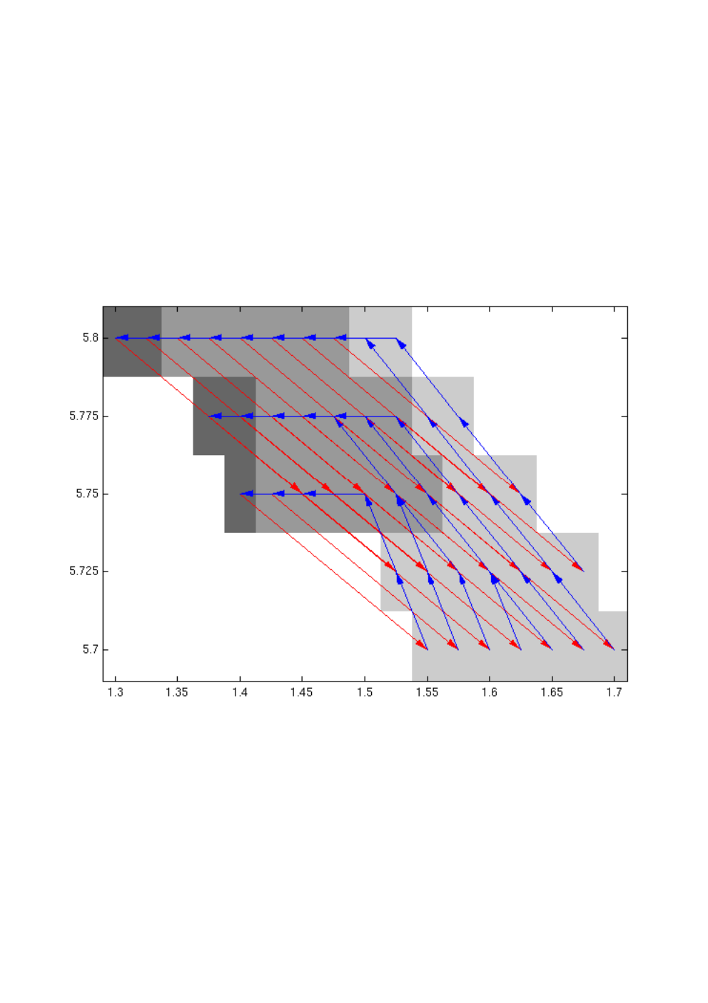
We consider two different values of the precision parameter . We first choose a precision which can be achieved by choosing . This precision is quite poor and makes the computed symbolic model of no practical use. However, it helps to understand the second experiment decribed further. On Figure 3, the symbolic model of the boost DC-DC converter is shown on the left, red and blue arrows represent the transitions associated with mode 1 and 2, respectively. We only represented the transitions that keep the state of the symbolic model in the set . Using supervisory control [RW87], we synthesized the most permissive controller that keeps the state of the symbolic model inside . It is shown on the right figure, the color of the boxes centered around the states of the symbolic model gives the corresponding action of the controller: dark and light gray means that for these states of the symbolic model the controller has to use mode 1 and 2, respectively; medium gray means that for these states the controller can use either mode 1 or mode 2; white means that from these states there does not exist any switching sequence that keeps the state of the symbolic model in , i.e. these states are uncontrollable. From this controller, using the approach presented in [Tab08], one can derive a controller for the boost DC-DC converter that keeps the state of the switched system in . Clearly, the chosen precision is too large to make this controller useful from a practical point of view.
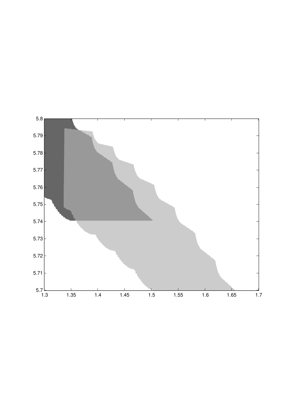
The second value we consider for the precision parameter is . This precision can be achieved by choosing . We do not show the symbolic model as it has too many states () to be represented graphically. We repeat the same experiment with this model, the most permissive controller that keeps the state of the symbolic model in is shown in Figure 4, on the left. The computation of the symbolic model and the synthesis of the supervisory controller, implemented in MATLAB, takes overall less than 60 seconds. From the controller of the symbolic model, we derive a controller for the boost DC-DC converter that keeps the state of the switched system in . We apply a lazy control strategy, when the controller can choose both modes 1 and 2, it just keeps the current operation mode unchanged. A state trajectory of the controlled boost DC-DC converter is shown in Figure 4, on the right. We can see that the trajectory remains in the invariant set.

5.2. Multiple Lyapunov functions
We now consider a second example inspired by a well known switched system with stable subsystems and exhibiting unstable behaviors (see e.g. [Lib03]). The system has two modes and the state space is . The dynamics associated with both modes are affine of the form () with
We consider a control design problem with a safety specification: the goal is to keep the trajectories of the switched system within a specified region of the state-space, denoted , while avoiding a specified subset of unsafe states . We assume that contains the equilibrium points of both systems and therefore the specification cannot be met by neither nor .
The system does not have a common -GAS Lyapunov function because it exhibits unstable behaviors for some switching signals (e.g. apply periodically mode during time unit, then mode during time unit and so on). However, each subsystem has a -GAS Lyapunov function of the form with
The corresponding -GAS Lyapunov functions have the following characteristics: , , . Moreover, the assumptions of Theorem 2.8 hold with , and a dwell-time . Here, again, the switched system is -GAS however it is not GAS because the subsystems do not share a common equilibrium point. Also, equation (2.8) holds on the entire state-space with . We set the sampling period to . Then, a symbolic model can be computed using the procedure described in Section 4.2. According to Theorem 4.2, a desired precision can be achieved by choosing a state space discretization parameter satisfying .
We choose , corresponding to a precision . Then, we used supervisory control to design the most permissive controller that keeps the state of the symbolic model within the set while avoiding . Though our symbolic model has states, the overall computation, including the determination of the symbolic model and the synthesis of the controller, takes only about seconds.
The controller is shown on Figure 5. On the left, respectively on the right, we represented the possible control actions when the current mode is , respectively , and the dwell time has elapsed (i.e. switching is enabled). Dark and light gray means that for these states of the symbolic model the controller has to use mode 1 and 2, respectively; medium gray means that for these states the controller can use either mode 1 or mode 2; white means that these states are uncontrollable and the specification cannot be met from these states.


From the most permissive controller represented on Figure 5, we designed a lazy controller for the symbolic model. Unlike the most permissive controller, the lazy control strategy can be implemented regardless of the current mode and of the time elapsed since the latest switching. The controller is represented on Figure 6, on the left: dark and light gray means that for these states of the symbolic model the controller has to use mode 1 and 2, respectively; medium gray means that for these states the controller must keep the current mode unchanged; white means that these states are uncontrollable. Let us remark that by design, this controller satisfies the dwell time constraint though it does not appear explicitely in the controller description. Using the approach presented in [Tab08], one can derive a controller for the switched system, that keeps the state of the switched system within the set while avoiding . On Figure 6, in the center, we represented an example of switching signals generated by the controller and the corresponding evolution of the state variables. We can check that the switching signal indeed has dwell time . On the right, we represented the associated trajectory of the switched system, satifying the safety property.


6. Conclusion
In this paper, we showed, under assumptions ensuring incremental stability, such as existence of a common -GAS Lyapunov function or multiple -GAS Lyapunov functions with dwell time, the existence of approximately bisimilar symbolic abstractions for switched systems. The proof of existence is constructive: these abstractions are effectively computable and any precision can be achieved. Two non-trivial examples of controller design based on symbolic models of switched systems have been shown.
The authors are currently improving the presented results in two different directions. The controllers resulting from arbitrary specifications may require switching surfaces with complex geometries. This increases the space complexity of controllers and complicates its real-time implementation. To address this difficulty, the authors are currently investigating the synthesis of more conservative controllers that are guaranteed to have lower complexity switching regions. The other direction being investigated is the most efficient enforcement of the dwell time requirement. Instead of building this requirement in the symbolic model, which results in larger symbolic models, it is possible to incorporate this requirement as part of the overall specification. We can thus synthesize controllers based on smaller symbolic models while meeting all the dwell time requirements.
References
- [Ang02] D. Angeli. A Lyapunov approach to incremental stability properties. IEEE Trans. on Automatic Control, 47(3):410–421, March 2002.
- [AS99] D. Angeli and E.D. Sontag. Forward completeness, unboundedness observability, and their Lyapunov characterizations. Systems and Control Letters, 38(3):209–217, 1999.
- [AVW03] A. Arnold, A. Vincent, and I. Walukiewicz. Games for synthesis of controllers with partial observation. Theoretical Computer Science, 28(1):7–34, 2003.
- [BPM05] A.G. Beccuti, G. Papafotiou, and M. Morari. Optimal control of the boost dc-dc converter. In IEEE Conf. on Decision and Control, pages 4457–4462, 2005.
- [BPM06] A.G. Beccuti, G. Papafotiou, and M. Morari. Explicit model predictive control of the boost dc-dc converter. In Analysis and Design of Hybrid Systems, pages 315–320, 2006.
- [BRC05] J. Buisson, P.Y. Richard, and H. Cormerais. On the stabilisation of switching electrical power converters. In Hybrid Systems: Computation and Control, volume 3414 of LNCS, pages 184–197. Springer, 2005.
- [GP07] A. Girard and G.J. Pappas. Approximation metrics for discrete and continuous systems. IEEE Trans. on Automatic Control, 52(5):782–798, 2007.
- [GPT08] A. Girard, G. Pola, and P. Tabuada. Approximately bisimilar symbolic models for incrementally stable switched systems. In Hybrid Systems: Computation and Control, volume 4981 of LNCS, pages 201–214. Springer, 2008.
- [Kha96] H.K. Khalil. Nonlinear Systems. Prentice Hall, 1996.
- [Lib03] D. Liberzon. Switching in Systems and Control. Birkhauser, 2003.
- [Mil89] R. Milner. Communication and Concurrency. Prentice Hall, 1989.
- [Par81] D.M.R. Park. Concurrency and automata on infinite sequences. In GI-Conf. on Theoretical Computer Science, volume 104 of LNCS, pages 167–183. Springer, 1981.
- [PGT07] G. Pola, A. Girard, and P. Tabuada. Approximately bisimilar symbolic models for nonlinear control systems. In IEEE Conf. on Decision and Control, 2007.
- [PW96] L. Praly and Y. Wang. Stabilization in spite of matched unmodeled dynamics and an equivalent definition of input-to-state stability. Math. Control Signals Systems, 9:1–33, 1996.
- [RW87] P.J. Ramadge and W.M. Wonham. Supervisory control of a class of discrete event systems. SIAM Journal on Control and Optimization, 25(1):206–230, 1987.
- [SEK03] M. Senesky, G. Eirea, and T.J. Koo. Hybrid modelling and control of power electronics. In Hybrid Systems: Computation and Control, volume 2623 of LNCS, pages 450–465. Springer, 2003.
- [Tab06] P. Tabuada. Symbolic control of linear systems based on symbolic subsystems. IEEE Trans. on Automatic Control, 51(6):1003–1013, June 2006.
- [Tab08] P. Tabuada. An approximate simulation approach to symbolic control. IEEE Trans. on Automatic Control, 2008. To appear.