Imbalanced superfluid state in an annular disk

Before exploring the properties of imbalanced superfluid in the annular disk geometry, we first consider the 1D ring, which may be viewed as the limiting case where the disk width is so narrow that only one radial mode is relevant. This case has been studied by a number of authors. In the mean field(MF) level, a rigorous analysis for the 1D BdG equation is given in Ref. [19] in the presence of a magnetic field. In terms of 1D Luttinger liquid theory the imbalanced superconducting state is also elucidated by Yang [20], and very recently, the density matrix renormalization group algorithms are implemented on the 1D negative-$U$ Hubbard model to explore the FFLO state in Refs. [21, 22, 23, 24]. The cold fermionic gases with attractive interaction and population imbalance are studied theoretically in Ref. [25] and and Ref. [26].

In this subsection, we follow the MF treatment to give a brief description to the 1D imbalanced superfluid state. We consider a canonical ensemble and fix the number of fermions of different species. Although only the quasi-long range order may exist in 1D system, the MF approach presented in this section is helpful to understand the imbalanced superfluid in 2D annular disk geometry shown in later sections.

The mean field Hamiltonian for a 1D interacting system reads

$\hat{\psi}_{\alpha}(x)$ is the fermion annihilation field at position $x$ with spin index $\alpha$, $\Delta(x)$ is the fermion pairing field, $m$ is the mass of the particle, and $g<0$ is the attractive interaction strength. $\mu_{\alpha}$ are the Lagrangian multipliers or the chemical potentials, which are used to fix the numbers of fermions of different spins at $N_{\uparrow}$ and $N_{\downarrow}$, respectively.

Eq. (1) has the similar form to the well known Su-Schrieffer-Heeger(SSH) model [27] for polyacetylene, which describes a 1D electron system coupled to phonons. In this system, when the phonon fields are condensed in opposite phases at the two ends of the 1D string, there are possible soliton excitations with zero energy in the fermion spectrum. The soliton excitations are also possible in the 1D superfluid Hamiltonian Eq. (1), where the MF pairing parameter $\Delta(x)$ can mimic the phonon field in the SSH model, which is shown briefly below. More details can be found, e.g., in Ref. [19]. For simplicity we take $\mu_{\uparrow}=\mu_{\downarrow}=\mu$, which determines the Fermi momentum $k_{F}=\sqrt{2m\mu}/\hbar$. The low energy physics is described by quasiparticles around the two Fermi points $\pm k_{F}$, i.e., the following decomposition is allowed

with left and right movers defined as

$\Lambda$ is a suitable momentum cutoff. These quasiparticle operators satisfy the standard anti-commutation relations, i.e.,

and all the other anti-commutators are zero. Substituting Eq. 2 into Eq. 1, and neglecting the fast oscillation terms ($\propto\exp(\pm 2ik_{F}x)$), one obtains the following two Hamiltonians to the linear order of $k$,

Here $:A:$ denotes normal ordering of $A$ and $v_{F}$ means the positive Fermi velocity. In the following $\hbar v_{F}$ is taken as unit. $\hat{H}_{1}$ and $\hat{H}_{2}$ are commutative with each other, and connected through the gap equation

The order parameter $\Delta(x)$ is assumed to be real. Eq. 5 shows that the pairing takes place either between $\hat{L}_{\uparrow}$ and $\hat{R}_{\downarrow}$, or between $\hat{L}_{\downarrow}$ and $\hat{R}_{\uparrow}$. Actually, $\left\langle R_{\downarrow}L_{\uparrow}\right\rangle=\left\langle L_{\downarrow}R_{\uparrow}\right\rangle$ by symmetry. Formally, one may have $\hat{H}\sim\hat{H}_{1}+\hat{H}_{2}-\int dx|\Delta(x)|^{2}/g$, but it is emphasized that $\hat{H}_{1,2}$ only describe the low energy excitations near the Fermi surface.

Let’s consider only $H_{1}$ with a twisted $\Delta(x)$, i.e., $\Delta(-\infty)=-\Delta(\infty)=\Delta_{0}$. As shown by Jackiw and Rebbi[28], there is at least one zero mode $\hat{\gamma}_{0\uparrow}$ in the middle of the gap, which is localized in space and reads

It is easy to verify the commutation relation $[\hat{\gamma}_{0\uparrow},\hat{H}_{1}]=0$. Besides this localized zero mode, we also have other quasiparticle excitations $\hat{\gamma}_{n\alpha}$ in the continuum region, where $n$ and $\alpha$ are the energy level and spin indices, respectively. Assuming all of them constitute a complete representation of the Hamiltonian $H_{1}$, the lowest energy states are doubly degenerate in the presence of an order parameter with kink pattern, which is the spinless vacuum of the quasiparticles $\hat{\gamma}_{n\alpha}$ together with the zero mode $\hat{\gamma}_{0\uparrow}$ being either filled or empty. Similar analysis is also valid for the $H_{2}$ branch, for which one can find that the zero mode has the form

which satisfies $[\gamma_{0\downarrow},H_{2}]=0$.

In terms of $\hat{R}_{\sigma}$ and $\hat{L}_{\sigma}$, the total particle number $\hat{N}$ and total spin operator $\hat{S}$ can be written as

where the fast oscillating terms are neglected. Note that the quasiparticle operators $\hat{R}_{\sigma}$ and $\hat{L}_{\sigma}$ can only describe the low energy physics, hence the operator $\hat{N}_{\sigma}$ with normal ordering only measures the particle number relative to the Fermi surface. Obviously, unlike the SSH model[27] and the Jackiw-Rebbi model[28], the charge conservation is broken in the BCS theory, therefore one can not tell how many charges the soliton can carry. Despite this fact, the total spin is still a conserved quantity in our MF treatment, therefore each zero mode may carry half spin as an analog to the half charge investigated in Ref.[27, 28]. But in practice only one spin can be observed at the kink of $\Delta(x)$, since there are two branches of fermions($H_{1}$ and $H_{2}$). To observe the half spin, one must get rid of the fermion doubling problem. Nevertheless, this provides a mechanism to accommodate excess spins with zero energy. The total energy of the soliton measured relative to the uniform BCS state is computed to be $2\Delta_{0}/\pi$[29, 30], which is less than the superfluid gap.

For equally populated species $N_{\uparrow}=N_{\downarrow}$, the lowest energy state is obviously the BCS state with uniform pairing gap. If one spin is flipped from downward to upward, i.e., $N_{\uparrow}+1$ up spin and $N_{\downarrow}-1$ down spin, a pair of soliton and anti-soliton is developed to store these two excess spins. We define the spin imbalance $n$ to be $(N_{\uparrow}-N_{\downarrow})/2$ for spin 1/2 particle. A typical soliton and anti-soliton pair is plotted in Fig. (1a), which is obtained by numerically solving Eq. (1) in a ring, where we use the angle $\theta=2\pi x/L$ as the coordinate. Due to the periodic boundary condition, a single soliton can not exist freely so that it must co-exist with an anti-soliton as a pair with the same width $\xi$. We call these soliton states with each spin per soliton (anti-soliton) as ideal soliton state. Note that since the order parameter is real, this state is also a kind of LO state. Actually, all the self-consistent solutions shown in this paper have real order parameters which minimize the energy, and therefore they are LO state. In the following sections, we omit “LO” for the sake of brevity.

With the increase of the flipped spins, more soliton and anti-soliton pairs are generated. Thus we get the soliton lattice state with $n$ pairs of soliton and anti-soliton as long as the system is in the dilute limit by which we mean $n\xi\ll 2\pi$, here the soliton width $\xi$ is measured in unit of the angle. In the dilute limit, the solitons are well separated from each other, which has two consequences (i) all the midgap states have zero energy, and (ii) each soliton or anti-soliton carries exactly one localized spin. According to these two properties, we distinguish soliton lattice state from the sinusoidally modulated state, where the spin imbalance $n$ is too large to satisfy $n\xi<2\pi$ and solitons overlap considerably with each other. Then the energy spectrum of the midgap states has a dispersion described by the Bloch theorem for a periodic lattice. Such a scenario from soliton lattice to sinusoidally varying state has also been addressed in Ref. [31] from the viewpoint of GL theory. The pairing parameter for both states can be described perfectly by the fitting function $\tilde{\Delta}\tanh(\cos n\theta/\tilde{\xi})$ ¹¹ 1 The soliton lattice pattern of pairing parameter can be described by Jacobi elliptic function as done in Ref. [19], but we do not take that expression for the sake of simplicity. with $\tilde{\Delta}$ and $\tilde{\xi}$ to be determined, which is shown in Fig. 1.

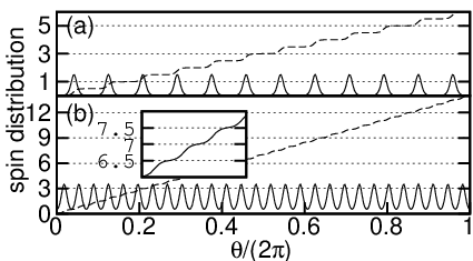
We now introduce two spin distribution functions, local spin distribution $S_{L}(\theta)=\frac{1}{2}\langle\hat{\psi}^{\dagger}_{\uparrow}(\theta)\hat{\psi}_{\uparrow}(\theta)-\hat{\psi}^{\dagger}_{\downarrow}(\theta)\hat{\psi}_{\downarrow}(\theta)\rangle$ as well as integrated spin distribution $S_{I}(\theta)$,

As shown in Fig. 2, the localization of spin density in the soliton lattice state manifests itself in the plateau features of the function $S_{I}(\theta)$. For the sinusoidally modulated state, the plateaus disappear due to the delocalization of spins.

Here we introduce $\mathcal{Q}$ to denote the number of spins per soliton/antisoliton. In the previous subsections, we focused on the state with only one spin($\mathcal{Q}=1$) per soliton. Now we study the case for $\mathcal{Q}\geq 2$, which we call deformed soliton state. Firstly, let us consider the case for odd $\mathcal{Q}$. The order parameter of a deformed soliton state for $\mathcal{Q}=3$ is plotted in Fig. 3(solid lines), which corresponds to 6 excess spins in total. Note that these 6 spins can also be stored in 3 ideal soliton-antisoliton pairs(dashed lines). Hence, we need to compare their energies numerically. It turns out that the deformed soliton is energetically favorable for strong interaction, while the ideal soliton state is preferable for weak interaction. Note that the deformed soliton found in this article has $\mathcal{Q}$ nodes in a narrow region. In fact $\mathcal{Q}$ spins can also be accommodated by a special soliton with only one nodes, which is described by $\Delta_{0}\tanh(x/\xi)$ with $\Delta_{0}\xi=(\mathcal{Q}+1)/2$(see Ref.[30]), however one can show that this solution is not energetically favored by comparing its energy and that of the corresponding well separated multi-soliton state.

In Fig. 3, the upper panel corresponds to a strong interaction case where the three spins are squeezed in a very narrow region with width comparable to that of an ideal soliton $\xi$. The total width is then estimated to be around $2\xi$, which is much smaller than the width $6\xi$ for the ideal soliton state. Thus, one can reasonably believe that the deformed soliton state has lower energy. If the interaction strength $g$ becomes weaker, as shown in the lower panel of Fig. 3, the deformed soliton with $\mathcal{Q}=3$ will inflate and its pattern is getting close to three ideal solitons. When $g$ becomes weak enough, the deformed soliton can not be stable, and is transmuted into an ideal soliton lattice state. The pairing order parameter shown in Fig. 3 can be perfectly fitted with function $\tilde{\Delta}_{0}[\tanh(\cos(\theta-\theta_{0})/\tilde{\xi}_{0})-\tanh(\cos(\theta)/\tilde{\xi}_{0}+\tanh(\cos(\theta+\theta_{0})/\tilde{\xi}_{0}]$ with three parameters $\tilde{\Delta}_{0}$, $\tilde{\xi}_{0}$ and $\tilde{\theta}_{0}$.

Note that the order parameter has a sign change $(-1)^{\mathcal{Q}}$ after crossing $\mathcal{Q}$ ideal solitons and antisolitons. Therefore, if $\mathcal{Q}$ is odd, a deformed soliton can be continuously transmuted into $\mathcal{Q}$ ideal solitons, but this is not true for even $\mathcal{Q}$ due to the mismatched boundary condition of $\Delta(x)$. In addition, the energy of a deformed soliton with even $\mathcal{Q}$ is not energetically favorable in our numerical calculations. Therefore, we do not need to consider the case for even $\mathcal{Q}$.

So far we only consider the system with fixed particle number, and have not included the magnetic field in our analysis. Since the total spin is a good quantum number, the effect of magnetic field can be easily estimated by simply adding Zeeman energy $-\mu_{B}h(N_{\uparrow}-N_{\downarrow})$. Obviously, the state with more excess spins gains magnetic energy, however it is at the cost of the deformation of pairing gap which loses the condensation energy. Therefore, the ground state should correspond to an optimized value of spin imbalance.

Let $n=(N_{\uparrow}-N_{\downarrow})/2$ be the spin imbalance, and the corresponding ground state energy be denoted by $E(n)$. The energy of the BCS state without spin imbalance is thus $E(0)$. Given an external magnetic field $h$, we then need to find the lowest free energy for all possible $n$’s, i.e., minimize $E(n)-2n\mu_{B}h$ with respect to $n$, which leads to an optimal spin imbalance $n_{c}$.

To this purpose, we define the energy cost per spin as

which can also be regarded as the energy cost for creating one soliton. The numerical data of $\varepsilon(n)$ is plotted in Fig. 4. As $n$ increases, the adjacent kinks become closer, which enhances the hopping amplitude of spins between kinks and consequently favors the kinetic energy of spin transfer. However, at the same time, the pairing gap gets smaller, which reduces the condensation energy. Thus the interplay between these two mechanisms leads to the nontrivial pattern of $\varepsilon(n)$ in Fig. 4.

There is a critical value $h_{1}$ of the magnetic field, below which the magnetic energy can not support an ideal soliton, and the system remains in the uniform state. When $h>h_{1}$, the sinusoidally varying state with modulation frequency $n_{c}$ will become energetically favorable. $n_{c}$ can be determined by the minimum of $2n\varepsilon(n)-2n\mu_{B}h$, alternatively, the optimal spin imbalance $n_{c}$ should satisfy

After a little algebraic analysis of Eq. (9), one can see that $n_{c}$ increases as $h$ increases. The first appeared $n_{c}$ is determined by $\epsilon(n_{c})=\mu_{B}h_{1}$ which is far from zero as shown in Fig. 4 and corresponds to a sinusoidally modulated state.

In this subsection, we show the numerical results in the grand canonical ensemble with fixed chemical potentials. For weak magnetic field($2\mu_{B}h=\mu_{\uparrow}-\mu_{\downarrow}$), the Zeeman energy is not enough to break the $s$-wave Cooper pairs, so the system retains the uniform BCS state. Until the magnetic field $h$ exceeds its first critical value $h_{1}$, the sinusoidally-varying LO state emerges. As the magnetic field is further increased, the modulation frequency of the order parameter becomes larger while its magnitude is reduced, until the system enters into the normal state at the second critical magnetic field $h_{2}$. We plot modulation frequency as a function of $h$ in Fig. 10, where one can find plateaus, since there should be integral pairs of domain walls in a ring geometry.

The phase separation(deformed domain wall) state can not be a ground state in the homogeneous magnetic field, except at the critical value $h_{1}$ of magnetic field. Furthermore, unlike the case of fixing particle number, there is no continuous crossover from domain wall state to the sinusoidally-varying state. The onset frequency at the critical magnetic field $h_{1}$ is finite and large enough to form a sinusoidally-varying LO state. The reason is that, to sustain a single domain wall, its magnetic energy gain must fully compensate the energy loss due to the deformation of pairing gap. In such a case there can be more domain walls. However the overlap of domain walls suppresses the pairing gap inevitably, which causes the loss of the condensate energy(see sec. 2.4). At the balance point of these two processes, sinusoidally-varying state shows up accompanied with delocalized spins.

References

- [1] Fulde P and Ferrell R A. Phys. Rev., 135:A550, 1964.
- [2] Larkin A I and Ovchinnikov Yu N. Sov. Phys. JETP, 20:762, 1965.
- [3] Matsuda Y and Shimahara H. J. Phys. Soc. Jpn., 76:051005, 2007.
- [4] Radovan H A, Fortune N A, Murphy T P, Hannahs S T, Palm E C, Tozer S W, and Hall D. Nature, 425:51, 2003.
- [5] Bianchi A, Movshovich R, Capan C, Pagliuso P G, and Sarrao J L. Phys. Rev. Lett., 91:187004, 2003.
- [6] Capan C, Bianchi A, Movshovich R, Christianson A D, Malinowski A, Hundley M F, Lacerda A, Pagliuso P G, and Sarrao J L. Phys. Rev. B, 70:134513, 2004.
- [7] Watanabe T, Kasahara Y, Izawa K, Sakakibara T, Matsuda Y, van der Beek C J, Hanaguri T, Shishido H, Settai R, and Onuki Y. Phys. Rev. B, 70:020506(R), 2004.
- [8] Miclea C F, Nicklas M, Parker D, Maki K, Sarrao J L, Thompson J D, Sparn G, and Steglich F. Phys. Rev. Lett., 96:117001, 2006.
- [9] Kumagai K, Saitoh M, Oyaizu T, Furukawa Y, Takashima S, Nohara M, Takagi H, and Matsuda Y. Phys. Rev. Lett., 97:227002, 2006.
- [10] Zwierlein M W, Schirotzek A, Schunck C H, and Ketterle W. Science, 311:492, 2006.
- [11] Zwierlein M W, Schunck C H, Schirotzek A, and Ketterle W. Nature, 442:54, 2006.
- [12] Partridge G B, Li W, Kamar R I, Liao Y A, and Hulet R G. Science, 311:503, 2006.
- [13] Partridge G B, Li W, Liao Y A, Hulet R G, Haque M, and Stoof H T C. Phys. Rev. Lett., 97:190407, 2006.
- [14] Shin Y, Zwierlein M W, Schunck C W, Schirotzek A, and Ketterle W. Phys. Rev. Lett., 97:030401, 2006.
- [15] Mizushima T, Machida K, and Ichioka M. Phys. Rev. Lett., 94:060404, 2005.
- [16] Machida K, Mizushima T, and Ichioka M. Phys. Rev. Lett., 97:120407, 2006.
- [17] Chen Y, Wang Z D, Zhang F C, and Ting C S. Phys. Rev. B, 79:054512, 2009.
- [18] Yanase Y. arXiv:cond-mat/0902.2275v1, 2009.
- [19] Machida K and Nakanishi H. Phys. Rev. B, 30:122, 1984.
- [20] Yang K. Phys. Rev. B, 63:140511(R), 2001.
- [21] Feiguin A E and Heidrich-Meisner F. Phys. Rev. B, 76:220508(R), 2007.
- [22] Rizzi M, Polini M, Cazalilla M A, Bakhtiari M R, Tosi M P, and Fazio R. Phys. Rev. B, 77:245105, 2008.
- [23] Tezuka M and Ueda M. Phys. Rev. Lett., 100:110403, 2008.
- [24] Feiguin A E and Heidrich-Meisner F. Phys. Rev. Letts., 102:076403, 2009.
- [25] Orso G. Phys. Rev. Lett., 98:070402, 2007.
- [26] Hu H, Liu X-J, and Drummond P D. Phys. Rev. Lett., 98:070403, 2007.
- [27] Su W P, Schrieffer J R, and Heeger A J. Phys. Rev. Lett., 42:1698, 1979.
- [28] Jackiw R and Rebbi C. Phys. Rev. D, 13:3398, 1976.
- [29] Dashen R F, Hasslacher B, and Neveu A. Phys. Rev. D, 12:2443, 1975.
- [30] Takayama H, Lin-Liu Y R, and Maki K. Phys. Rev. B, 21:2388, 1980.
- [31] Buzdin A I and Kachkachi H. phys. Lett. A, 225:341, 1997.
- [32] Vorontsov A B, Sauls J A, and Graf M J. Phys. Rev. B, 72:184501, 2005.