Dynamical pattern formation during growth of a dual-species Bose-Einstein condensate
Abstract
We simulate the growth of a dual species Bose-Einstein condensate using a Gross-Pitaevskii equation with an additional gain term giving rise to the growth. Such growth occurs during simultaneous evaporative cooling of a mixture of two gases. The ground state of a dual condensate is normally either a miscible mixture, or an immiscible phase with two spatially separated components. In a cigar trap the ground state typically consists of one component in the center, and the other component flanking it. Our simulations show that when the condensates are formed in a cigar trap and the mixture is phase separated, then the final state upon the end of the growth is generally far from the true ground state of the system. Instead it consists of multiple, interleaved bubbles of the two species. Such a pattern was observed recently in an experiment by Wieman’s group at JILA [1], and our simulations are in good qualitative agreement with the experiment. We explain the pattern formation as due to the onset of modulation instability during growth, and study the dependence of the final state pattern on various parameters of the system.
I INTRODUCTION
Like common fluid mixtures, dual species Bose-Einstein condensates (BECs) may exhibit both miscible and immiscible phases. In the miscible phase, the two species form a homogeneous solution, while in the immiscible phase, they separate spatially [2, 3]. In a BEC, the occurrence of these phases is controlled by the ratio of the inter-component interaction to that of the intra-component interactions.
The ground state structure of the immiscible phase is typically that of a ball and shell where one species forms a shell around the other, or that of two condensates lying side by side. In a quasi-1D trap, the structure can be of one component flanked by the other. The exact structure depends on the shape of the trap, the size of each component, and the interactions between them. In general, the two components tend to minimize the surface area that separates them, as this surface contributes surface tension energy [3, 4, 5, 6, 7].
By starting from the ground state of a miscible phase and increasing the inter-component repulsion (relative to the intra-component interactions), it is possible to make a transition from the miscible to the immiscible phase. Such a change in the interactions can bring about a modulation instability where the two components separate locally and form a pattern of interleaved bubbles. Alternatively, such a pattern emerges when half the population of one pure component is suddenly transfered to another one, and the two components separate [8, 9, 10].
A recent experiment [1] on a mixture of 85Rb and 87Rb in an elongated cigar trap, observed an intriguing modulated pattern upon the end of evaporative cooling (shown in figure 4 of that reference). The pattern is that of separated and interleaved “bubbles” of the two components, with up to 3-4 bubbles from each component. This behavior is seen when the inter-component repulsion is strong compared to the intra-component interactions, i.e, when an immiscible phase is expected.. These specific patterns were observed even under conditions when the interactions strengths were kept constant during and after the evaporative cooling. Nor is there population transfer involved, as the two components are different isotopes. Following evaporative cooling one may then expect to obtain a binary condensate in its ground state. But the observed modulated pattern does not look like the ground state of the system.
In this paper we suggest that the emergence of this pattern has to do with the dynamics of the formation of the binary condensate during the evaporative cooling. When the condensates are formed they are initially very small. Their mutual interaction (proportional to the densities) is then weak and we expect them to coexist spatially, even when the predicted phase for a Thomas-Fermi (large number of atoms) regime is immiscible. As the condensates grow, spatial separation is triggered by the growing inter-component repulsion. One may expect this to bring about a modulation instability giving rise to the final observed spatial pattern.
Our aim in this paper is to demonstrate this mechanism, predict the conditions for the formation of the spatial structure, and determine the factors that influence the number of bubbles formed. The paper is organized as follows: in section (II) we give the theoretical background: we present the Gross-Pitaevskii gain model for a double condensate, and review the theory of modulation instability mechanism. In section (III) we present and discuss the results of our numerical simulations. We summarize our conclusions in section (IV).
II BINARY CONDENSATE GROWTH MODELING
II.1 Gross-Pitaevskii Gain model
We are interested in the dynamics of the formation and growth of the binary condensate during the evaporative cooling, in order to understand the final spatial pattern that emerges. The description of BEC growth is a challenging theoretical problem. In principle it is possible to perform first-principles numerical simulations of the relevant equations [11, 12]. However, a great deal of physical insight can be obtained from a simpler model. In the first instance, the thermal cloud is much more dilute than the condensate. Therefore, it is plausible to treat the system as a two fluid model, where the thermal component is assumed to be an ideal gas and its interactions with the condensate are neglected. If one is only interested in the condensate, then the role of the thermal component is simply that of a particle reservoir feeding the growing condensate. One thus arrives at the Gross-Pitaevskii gain model [13]. This is a Gross-Pitaevskii equation modified by a linear gain term. For two components, the Gross-Pitaevskii gain equations (GPGE) read:
| (1a) | |||||
| (1b) | |||||
Here, and are the wavefunctions corresponding to the two condensates. The normalization of each wavefunction is taken independently as . and are the corresponding atomic masses. The condensates are assumed to be trapped in axis-symmetric harmonic potentials,
| (2) |
where are the radial and transverse trapping frequencies, and the axial center of the traps. We allow for the possibility of different axial trapping frequencies for the two condensates, as well as for a relative axial shift between the centers of the traps, as occurs in the experiment [1].
The intra-component coupling constants are characterized by the scattering lengths and between atoms of the same species, while the inter-component coupling, , (with ), is determined by the scattering length , where an atom of component 1 scatters from an atom of component 2. The ’s are the gain terms. They contribute to the growth of component within timescale 1/. Intuitively, the growth terms arise from boson statistics, where the probability to add an additional atom to condensate is proportional to the number of atoms already condensed. In practice these are phenomenological parameters and may be estimated by fitting to an experiment.
II.2 Modulation Instability Mechanism
Following the analysis of Refs. [6, 5, 1] we define the parameter
| (3) |
that depends upon the ratio of the single species and interspecies interactions. When the number of atoms is large enough the system may be treated by the Thomas-Fermi approximation, which neglects the kinetic energy. Assuming , there are two regimes: , where the two condensates are miscible, and , where they are immiscible due to the interspecies repulsion.
It is important to bear in mind that this classification is correct only when the Thomas-Fermi approximation is valid. It does not hold for small, trapped condensates, where the kinetic energy terms are significant. In the numerical simulations presented in the next section we shall show that in this case the condensates can initially co-exist spatially even when . As they grow, spatial separation sets in. To have a better understanding of the dynamics of spatial separation, it is useful to consider an idealized system, of two homogeneous condensates in a quasi one dimensional geometry (relevant to the experiment [1]), with respective densities and , co-existing spatially at time , as discussed in detail in Refs. [9, 10]. If , the system is stable. If , the initial state is unstable, and an initially homogeneous system will evolve dynamically. In this so called modulation instability mechanism, the two components separate, and the separation occurs in a wave pattern with a typical length scale which depends on the relative interactions and densities. Regions of over-density of one component appear in regions of under-density of the other component, and vice versa. Nonlinearity accelerates the process and brings about complete spatial separation. A pattern of interleaved bubbles of the two components emerges. The final spatial pattern can be very stable, since there is no room for movement to “the sides”, and the energy barrier for tunneling between the separated bubbles is very big.
The analysis of the modulation instability in a dual component BEC in a quasi 1D geometry was done in Ref. [10]. There, the assumption of equal masses has also been made, which considerably simplifies the analysis. The behavior of the system at small can be deduced from the excitation spectrum. The eigenmodes of the system are characterized by a longitudinal wave number and frequency . For each eigenmode, the wave number is shared by the two components 11 1 In [10] the authors allowed for two independent wave numbers and for the two components. We note that actually must hold for the solution to be an eigenmode. Their results are correct as long as one takes =.. The instability manifests itself in a continuous range of modes which have imaginary frequencies. The most unstable mode is that with imaginary frequency of maximum absolute value. This is the mode that will grow fastest. Its wavenumber is found to be:
| (4) | |||||
where is the radial harmonic oscillator length , and we assume here .
The imaginary frequency of this mode is found to be:
| (5) |
and the time scale for growth is .
III NUMERICAL SIMULATIONS
III.1 Mechanism of dynamical phase separation
We have performed numerical simulations of the growth of the dual 85Rb/87Rb condensate based on Eq. (1). In correspondence with the experiment [1], all our simulations have the following fixed parameters. bohr is the scattering length of 87Rb. bohr is the inter-species scattering length. The trap parameters are: radial frequency Hz for both components; axial frequency Hz for 85Rb and Hz for 87Rb.
We first demonstrate that the true ground state of the system in an immiscible phase is indeed quite simple, as described above. We computed the ground state with , and the other scattering lengths fixed as above, so that . The ground state for this system with 50,000 atoms in each component is shown in Fig. (1). The calculation is 3D, and the figure shows the density profile along the long z-axis, where . We have also performed additional computations which modeled the effects of a gravitational sag that breaks the cylindrical symmetry and slightly shifts the centers of masses of the the two components. In all cases, the ground state was still similar in shape to that of Fig. (1).

We now investigate the consequences of a dynamical growth of a dual condensate during evaporative cooling. The exact growth time of the condensates in the experiment [1] is not known, but has been roughly estimated to be between 100-500 ms 22 2 J. Pino, private communication. In our simulations we begin with the ground state consisting of 10 atoms of each component, and let the condensates grow for 300ms. We choose gain terms , giving rise to a final population of 51,000 atoms in each component. The number of atoms of component at time can be calculated from: . We assume that after 300ms full condensation has been achieved and the growth is terminated. The ’s are then set to zero and further dynamics are atom number conserving. Fig. (2) shows stages in the growth of the dual condensate under these conditions. Animations of this evolution are available at http://grizzly.colorado.edu/ bohn/movies/bubbles.htm

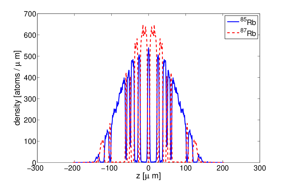
In the initial state (panel ), the number of atoms is very small so that the mean field interactions are weak. Each condensate’s shape is essentially Gaussian and they are almost perfectly overlapping. As the density grows (due to the imaginary gain term), the interactions kick in (around 130ms, compare panels and ), leading to phase separation at the center, where density is largest. After the end of the growth (at 300ms, panel ) the modulation pattern is observed to be quite stable, apart from a breathing motion, with the components almost fully separated and forming multiple interleaved bubbles, as shown in Fig. (3). Note the increasing vertical scales, which account for growing particle numbers.
The onset of the immiscibility is triggered by the emergence of the modulation instability. The natural wavelength of the modulation instability corresponds to the unstable mode with maximum imaginary amplitude. This is where is given by Eq. (4); for the purpose of using this equation, which assumes species with equal masses, we use the average mass of the two isotopes of Rb, neglecting their small mass difference. Also, for our non-homogeneous system, we use in it the maximum density of each component. As the density of the condensates grows, their spatial extent increases and at the same time the modulation instability wavelength decreases. The decrease of the modulation instability wavelength with time is shown in Fig. (4). Around 60ms after the beginning of the growth, the modulation instability wavelength becomes comparable to the size of the condensate as measured by the r.m.s of the density profile of the combined condensates. The onset of dynamical separation is seen somewhat later at 130ms. This lag in time may be due to two factors. Firstly, the MI wavelength Eq. (4) assumes a homogeneous condensate. In other words, it applies when the local density approximation (LDA) is valid. On the other hand, the number of atoms in each component at ms is only about 400. Thus, the LDA approximation is not yet reliable. Secondly, as we discuss below, there is a time scale associated with the growth of the unstable mode, and this leads to a lag between the initial seeding of the instability and its growth to an observable size. Nevertheless, the crossing of the curves of the r.m.s size of the condensate and the modulation instability wavelength indicates, to within a factor of two in time, the onset of the dynamical instability.
As condensation proceeds and the density continues to grow, the spatial extent of the condensates increases and at the same time the modulation instability wavelength decreases further. This leads to the continuous separation of the two components into smaller and smaller “bubbles”, as can be seen in Fig. (2). The final size of individual bubbles is determined by the point at which essentially complete spatial separation between the two components is achieved, so that no more sub-divisions are possible. The exact point at which this happens depends strongly on the non-linear dynamics and is thus difficult to estimate solely from the linear small perturbations analysis which is behind Eq. (4). Typically, the final modulation instability wavelength is much smaller than the size of the observed bubbles, but this has no effect since at this point the bubbles are already almost purely separated components.
Regarding the temporal evolution, we can compare two time scales. One is the time scale over which the condensate’s population grows, and the other is the time scale for the growth of the most unstable mode. This modulation instability time scale depends on the density and thus is itself time-dependent. Fig. (5) shows the evolution of the modulation instability time scale as function of the simulation time, where is given by Eq. (5). As the density of the condensate grows, the timescale for the growth of the most unstable mode is decreasing exponentially. Around 130ms the time scale of growth of the unstable mode becomes comparable to the time scale of growth of the condensates themselves. As we have seen, this coincides with the point where dynamical phase separation begins to be observable in the simulation. With increasing simulation time, the modulation instability growth time scale becomes very short, leading to the rapid appearance of bubbles between 180ms and 240ms in Fig. (2).


III.2 Factors affecting the spatial pattern formation
We explored some of the factors that affect the final spatial pattern upon the end of evaporative cooling. As noted above, the condition for phase separation in the Thomas-Fermi limit is where is defined in Eq. (3). We find that having a negative with larger absolute magnitude leads to the dynamical formation of fewer bubbles. For example, Fig. (6) shows the modulation pattern after 1000ms with the only difference from Fig. (3) that has been reduced from 200 to 81 bohr, so that , which for the previous case equals , is now . The number of separated bubbles is clearly reduced, from 25 in the first case to 17 in the second. The physical reason for this effect is as follows. When is more negative (larger absolute value), the dynamical phase separation begins earlier in the growth process when the size of the condensates is smaller. Since the size of the condensates is smaller, they divide into smaller number of bubbles. Saturation (that is, complete spatial separation of the two components) is also achieved earlier, and no further sub-division occurs at later times. On the other hand, with smaller absolute value of the condensates have a chance to increase there size before the onset of phase separation. Thus, eventually, when phase separation takes place, a larger number of bubbles can be formed.
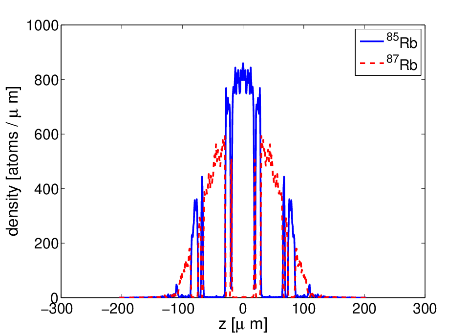
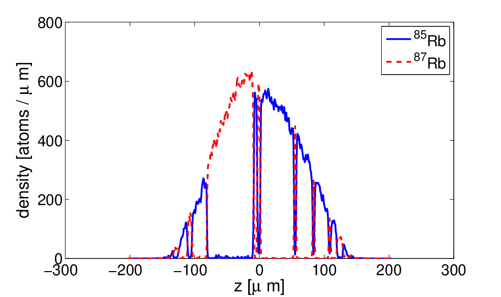
An even more dramatic effect is seen when the centers of the traps of the two components are shifted one from the other along their long axis by a small distance, as may occur due to residual gravitational sag. This can occur when the trap is slightly tilted off the horizontal to the earth, as apparently occurred in the experiment [1]. Even if the tilt is slight, the effect can be large in the axial direction due to the low and different trapping frequencies for the two components in this direction. This leads to asymmetry in the spatial pattern formation. Fig. (7) shows an asymmetrical pattern obtained with a dual condensate with the same interaction parameters as of Fig. (3), but with the centers of the traps of the two components shifted 1.7 m from each other. Fig. (8) shows the time dynamics leading to this pattern. The initial shift is clearly seen in the partial overlap between the “seed” Gaussian of the two components. As the density grows, the inter-component repulsion causes the centers of mass of the two components to move farther apart. At the same time, modulation instability and bubble formation occurs where the two components overlap. Due to the reduced spatial overlap (compared to the case with no shift of the traps’ centers), the final number of bubbles is much reduced.

We also note that the modulation instability mechanism which is at the heart of the spatial pattern formation requires a quasi one dimensional geometry. In a fully 3D trap (with aspect ratio close to one), even if “bubbles” are seeded, they would quickly merge and coalesce. This is because a spatial pattern which contains many bubbles would have higher energy then one with continuous, bulk configuration with no bubbles, due to the contribution of surface tension energy [7]. But, in the quasi 1D trap there is a high energy barrier for the merging of two bubbles of one component separated by a bubble of another component. This is essentially a tunneling process which is highly suppressed. Our numerical simulations support this picture. For example, we find that in a trap with aspect ratio (compared with in the simulations discussed above) it is quite hard to see bubbles, and at most four to five are formed.
Another factor in the growth dynamics concerns the start of condensation of the two components. When the atom numbers of the two components are the same, they have the same critical temperature and so may be expected to begin condensation at the same time. However when the two components contain different number of atoms, the critical temperature of the larger component is higher (), so it may be expected to begin condensation first. The time delay between the start of condensation of the two components will then depend on their atom number ratio and on the rate of evaporative cooling. We have performed simulations with large time delay such that one component begins to condense after the end of condensation of the second. We find that in this case the growth of the component which condenses later occurs at the edges of the first one, and they form a structure similar to the usual ground state, with no bubble pattern. This may be expected since the first component to condense creates a repulsive potential which repels the second component from condensing in the center of the trap. Thus, a sufficient temporal overlap between the condensation of the two components seems essential for formation of a bubble pattern.
III.3 Comparison with experiment
To make a concrete connection with the experimental results [1], we simulated as close as possible the conditions under which the remarkable bubble patterns seen in Fig.(4b) and (4c) of Ref. [1] were observed. The result is shown in Fig. (9). The number of atoms (reported in the caption) was also estimated from the experiment 33 3 J. Pino, private communication, with 87Rb atoms and 85Rb atoms. In this simulation we assume that the two components begin to condense together. Due to the different atom numbers this might not have been the case in the experiment, but should be good enough as long as the time delay between condensation of the two components is not too long. In the simulation We can see the formation of three bubbles of 85Rb immersed in and between the larger cloud of 87Rb. This result is qualitatively similar to that observed in the experiment. The comparison with the experiment is quite encouraging, especially bearing in mind that we do not know parameters such as the exact time(s) of the growth of the two condensates, and the initial condensate “seed” sizes. The condensates in the experiment also show evidence for gravitational sag. In the radial direction, gravitational sag breaks the cylindrical symmetry, an effect we have not attempted to simulate here. However we do include the effect of asymmetry in the axial direction due to residual gravity sag along this direction, which can occur due a slight tilting of the trap from the horizontal to the earth.

IV Conclusions
In this work we have put forward a mechanism which explains the intriguing experimental observations of [1]. These observations showed the formation of a spatial modulated pattern of a dual BEC condensate upon the end of evaporative cooling in an highly elongated cigar trap. The mechanism we suggest includes two crucial elements. One, the growth of the dual condensates which is modeled by imaginary gain terms in the Gross-Pitaevskii gain equation, Eq. (1). Second, as the condensates grow and their mutual interaction becomes more and more dominant, the mechanism of modulation instability kicks in, and gives rise to the evolution of spatial modulation with smaller and smaller wavelength. The initial linear instabilities are amplified by the non-linearity in the system, and this process comes to an end when full spatial separation between the two components is achieved. The final pattern is very long lived due to the large energy barrier for the separated component “bubbles” to cross over each other. The quasi 1D nature of the trap is essential, otherwise no barriers exist to prevent any formed “bubbles” from merging and coalescing into continuous, bulk components.
Naturally, the gain model is a simplified, phenomenological model of the growth of two coherent condensates from the thermal gases, which does not include the interactions between the condensates and the thermal gases, nor any direct temperature dependence. The thermal gas only enters through its role as a particle reservoir (for the gain terms). Thus, in principle, other mechanisms such as thermal fluctuations may also play a role in the final observed spatial pattern in the experiments. It would be of interest to have a more elaborate (but therefore, more complicated) modeling of the evaporative cooling process of a dual condensate. One such possible model may be the stochastic Gross-Pitaevskii equation [14] which recently was shown to give excellent agreement with the experimental observation of spontaneous vortex formation in evaporative cooling of a single component BEC [15]. Nevertheless, the encouraging agreement between our simulations and the experiment supports our belief that the simple model put forward here already captures the essential physics at the root of the observed phenomenon.
Acknowledgements.
S. R. and J. L. B. acknowledge financial support from NSF. M.E. and L.E.H. acknowledge support on NSF grants PHY-0354969 and PHY-0653359.References
- [1] S. B. Papp, J. M. Pino, and C. E. Wieman, arXiv:0802.2591 (2008).
- [2] C. J. Myatt, E. A. Burt, R. W. Ghrist, E. A. Cornell, and C. E. Wieman, Phys. Rev. Lett. 78, 586 (1997).
- [3] B. D. Esry, C. H. Greene, J. P. Burke, and J. L. Bohn, Phys. Rev. Lett. 78, 3594 (1997).
- [4] M. Trippenbach, K. Góral, K. Rza̧żewski, B. Malomed, and Y. B. Band, J. Phys. B 33, 4017 (2000).
- [5] D. M. Jezek and P. Capuzzi, Phys. Rev. A 66, 015602 (2002).
- [6] F. Riboli and M. Modugno, Phys. Rev. A 65, 063614 (2002).
- [7] B. V. Schaeybroeck, arXiv:0805.2512 (2008).
- [8] H. J. Miesner, D. M. Stamper-Kurn, J. Stenger, S. Inouye, A. P. Chikkatur, and W. Ketterle, Phys. Rev. Lett. 82, 2228 (1999).
- [9] K. Kasamatsu and M. Tsubota, Phys Rev. Lett. 93, 100402 (2004).
- [10] K. Kasamatsu and M. Tsubota, Phys. Rev. A 74, 013617 (2006).
- [11] P. D. Drummond and J. F. Corney, Phys. Rev. A 60, R2661 (1999).
- [12] P. B. Blakie and M. J. Davis, Phys. Rev. A 72, 063608 (2005).
- [13] P. D. Drummond and K. V. Kheruntsyan, Phys. Rev. A 63, 013605 (2000).
- [14] C. W. Gardiner and M. J. Davis, J. Phys. B 36, 4731 (2003).
- [15] C. N. Weiler, T. W. Neely, D. R. Scherer, A. S. Bradley, M. J. Davis, and B. P. Anderson, arXiv:0807.3323 (accepted for publication in Nature) (2008).