Supersymmetry with a Chargino NLSP and Gravitino LSP

In the MRSSM, gaugino masses arise from Eq. (1) which generate Dirac masses that pair the gauginos $\left(\tilde{g},\tilde{W}\;\text{and}\;\tilde{B}\right)$ with their fermionic partners $\left(\psi_{\tilde{g}},\psi_{\tilde{W}}\;\text{and}\;\psi_{\tilde{B}}\right)$. Higgsino masses arise from pairing Higgs superfields $H_{u}$ and $H_{d}$ with partner fields $R_{u}$ and $R_{d}$ through a pair of mass terms

$R_{d,u}$ transform identically to $H_{u,d}$ under the electroweak group, except that the $R$-charges are $2$ rather than $0$. This $R$-charge assignment forbids Yukawa-like couplings of the $R$-fields to the matter fields. Hence, only Higgses acquire electroweak symmetry breaking expectation values. Upon electroweak symmetry breaking, the electroweak gauginos mix with the Higgsinos (just like in the MSSM). For completeness, all the multiplets in the MRSSM described in Ref. [29] are listed in Table 1 along with their matter and $R$-charges.

Let us first investigate the neutralino mass matrix in the MRSSM. The $R$-charges determine which neutralinos mix with each other and provide a guiding principle to determine the gauge-eigenstate basis. The vector $N_{+}\equiv\left(\tilde{W}_{3},\tilde{B},\tilde{R}_{u}^{0},\tilde{R}_{d}^{0}\right)$ carries $R$-charge $+1$, while the vector $N_{-}\equiv\left(\psi^{0}_{\tilde{W}},\psi_{\tilde{B}},\tilde{H}_{u}^{0},\tilde{H}_{d}^{0}\right)$ carries a $R$-charge $-1$. Field rotations do not mix up fields with different $R$-charges. Hence, just like with charginos in the MSSM, two independent rotation matrices are required to diagonalize the mass matrix.

The Lagrangian for neutralino masses can be written in the gauge-eigenstate basis as

where the neutralino mass matrix is given as

Here $\langle H_{u}\rangle\equiv v_{u}$ and $\langle H_{d}\rangle\equiv v_{d}$ with $v_{u}^{2}+v_{d}^{2}=v^{2}/2\simeq(174\;{\rm GeV})^{2}$. Notice the apparently unusual location of the $\mu$-terms in Eq. (4) is a direct result of the Dirac nature of the neutralino mass matrix. The physical mass-squareds are given by eigenvalues of $M_{\tilde{N}}M_{\tilde{N}}^{\text{T}}$. There are four new parameters $\lambda_{u},\lambda_{d},\lambda_{u}^{\prime}$ and $\lambda_{d}^{\prime}$ that arise from the superpotential terms

These couplings are unnecessary to the structure of the MRSSM but are nevertheless allowed under all of the charge assignments. Various checks have been performed on Eq. (4) to verify that every entry in this mass matrix is correct, see Appendix B.

For charginos, the mass matrix is even simpler because of the conservation of electromagnetic charge as well as $R$-charge. In the MRSSM there are eight two-component fermions from the winos, Higgsinos, and $R$-fields. Based on the $R$-charges and the electromagnetic charges, the eight fermions can be grouped into following four different classes which do not mix among themselves:

These charges imply that the charginos pair up as

where the chargino mass matrices in our basis are

Since each of these matrices are diagonalized by bi-unitary transformations, four independent rotations are needed for the four vectors listed in Eq. (6) in order to diagonalize the mass matrices.

We are now ready to calculate the mass eigenstates under various assumptions about the parameters of the MRSSM. One qualitative difference from the MSSM is that the Dirac nature of the gauginos allows us to take the gaugino masses $M_{1},M_{2}$ and Higgsino masses $\mu_{u},\mu_{d}$ real and positive (rotating phases into the holomorphic masses for the scalar adjoints and the $\lambda$ parameters) [29]. Examining the gaugino mass matrices, we explore several limits where we can analytically demonstrate that the chargino is the NLSP and obtain a good estimate of the mass difference. Our first treatment is to take $\lambda_{u,d}=\lambda^{\prime}_{u,d}=0$. This is motivated in part to simplify our analysis, but also to emphasize that nonzero values of these couplings are not necessary to obtain a chargino lighter than the lightest neutralino. Further simplifications can result by taking the large $\tan\beta$ limit and the large $M_{1}$ limit. In Sec. 2.3 we generalize and expand the discussion, while still working at tree-level. As we will see, the lightest chargino can be significantly lighter than the lightest neutralino when the $\lambda$ couplings are present with ${\cal O}(g)$ values.

The gaugino mass matrices, Eqs. (4) and (8), simplify in the limit $\lambda_{u,d}=\lambda^{\prime}_{u,d}=0$. Here we will also take $\mu_{u}=\mu_{d}=\mu$, which will prove extremely convenient in our analytic analysis in this section. Equal Higgsino masses will also allow us to illustrate the contrast between the MSSM and the MRSSM. We are obviously not interested in the case where the bino is the lightest gaugino, hence we take large $M_{1}$, consistent with the motivations of Ref. [29]. Integrating out the bino and taking $\tan{\beta}\gg 1$, the neutralino and chargino mass matrices are given by

For charginos, in the case $\tan\beta>1$, we need only consider $M_{\chi_{2}}$ in order to find the lightest chargino mass.

The block diagonal form of $M_{\tilde{N}}$ in Eq. (9) shows that a pair of neutral Higgsinos acquire a (Dirac) mass $\mu$ and do not mix with the other neutralinos. This allows us to further simplify the neutralino mass matrix down to just the upper $2\times 2$ block. Here is the key analytical observation: The upper $2\times 2$ block of $M_{\tilde{N}}$ is identical to $M_{\chi_{2}}$, except that the off-diagonal element is smaller for the neutralino mass matrix. Simple $2\times 2$ diagonalization clearly shows that the lightest chargino is lighter than the lightest neutralino in both the Higgsino limit ($\mu<M_{1},M_{2}$) and the wino limit ($M_{2}<\mu,M_{1}$),

where $\Delta_{+}\equiv m_{\tilde{\chi}^{\pm}_{1}}-m_{\tilde{\chi}^{0}_{1}}$.

It is well known that the one-loop electromagnetic radiative correction increases the chargino mass [11, 12, 13, 14]. But, since the size of the mass difference shown above is not parametrically small compared to the loop contribution, the tree-level splitting can easily dominate so long as one of the diagonal elements does not far exceed the other.

The analytical results are strikingly confirmed by examining a larger region of the MRSSM parameter space numerically. In Figs. 2 and 2 we plot the contours of $\Delta_{+}$, the difference of the lightest chargino mass to the lightest neutralino mass. Fig. 2 explores the mostly-Higgsino limit and was generated by holding $\mu=150$ GeV and $\tan\beta=10$. Similarly, Fig. 2 explores the mostly-wino limit and was generated holding $M_{2}=150$ GeV and $\tan\beta=10$. The regions under the dashed lines in these Figures result in $m_{\tilde{\chi}^{\pm}_{1}}<101$ GeV at tree level and thus will be ignored from further consideration.

In these Figures, it is clear that a chargino is the lightest gaugino in the regions with $\Delta_{+}<0$. This occurs throughout the tree-level parameter space of the wino limit, shown in Fig. 2. Note that we have not included radiative corrections in these numerical results because a full calculation requires knowing the full spectrum of the model. Nevertheless, it is clear that in a wide range of parameter space, the tree-level mass difference is much larger than are expected from radiative corrections, demonstrating that the chargino can indeed be the NLSP.

The full parameter space of the MRSSM is much larger than the MSSM. To keep things manageable we consider the following simplifications: $\lambda_{u}=\lambda_{d}\equiv\lambda$ and $\lambda^{\prime}_{u}=\lambda^{\prime}_{d}\equiv\lambda^{\prime}$. Moreover, it will be useful to define the parameters $M_{\lambda}=\lambda v/2$ and $\tan\theta_{\lambda}=\lambda^{\prime}/\lambda$, analogous to the electroweak parameters $M_{W}=gv/2$ and $\tan\theta_{W}=g^{\prime}/g$. We use perturbation techniques on this mass-squared matrix to find approximate analytical expressions for neutralino masses.

Having demonstrated analytically that the chargino can be the NLSP in several limits, we now turn to analyzing a larger region of the MRSSM parameter space numerically. The neutralino and chargino masses are determined by nine parameters: $M_{1}$, $M_{2}$, $\mu_{u}$, $\mu_{d}$, $\tan\beta$, $\lambda_{u}$, $\lambda_{d}$, $\lambda_{u}^{\prime}$, and $\lambda_{d}^{\prime}$. As it is too cumbersome to do a complete scan, we restrict to the simplifications introduced in the previous subsection: $\lambda_{u}=\lambda_{d}=\lambda$ and $\lambda_{u}^{\prime}=\lambda_{d}^{\prime}=\lambda^{\prime}$. As before, we also trade the parameters $\lambda$ and $\lambda^{\prime}$ for the mass parameters $M_{\lambda}$ and the angle $\theta_{\lambda}$.

In the first part of this subsection we keep $M_{\lambda}$ and $\tan\theta_{\lambda}$ fixed and scan the rest of the parameter space in order to understand the variation of $\Delta_{+}$. Later we will choose a particular point in the $M_{1}$, $M_{2}$, $\mu_{u}$, $\mu_{d}$ and $\tan\beta$ space, and see the dependence of $\Delta_{+}$ on our choice of $M_{\lambda}$ and $\tan\theta_{\lambda}$.

Note that given renormalization group evolution of the superpotential parameters $\lambda$ and $\lambda^{\prime}$, evidently a natural choice is $\tan\theta_{\lambda}=\tan\theta_{W}$. We also use $M_{\lambda}=M_{W}$ to begin our discussion.

First, consider the case of equal Higgsino masses with $\tan\beta=10$. (The one heavy Higgsino scenario, as we described before, is similar to the equal Higgsino scenario at sizeable $\tan\beta$). In Fig. 4 we hold $\mu$ constant and vary $M_{2}$ and $M_{1}$. The shape of the contours are the same as in Fig. 2, where we neglected the “$\lambda$” couplings. The striking difference is that now the mass difference ($\Delta_{+}$) can be as large as $-30$ GeV. In fact, this is why we chose $\mu=200$ GeV, so that the lightest chargino remains above the LEPII limit. In Fig. 4, the same analysis is repeated in the wino limit, with $M_{2}=200$ GeV, where again we see that mass difference $\Delta_{+}$ is negative and can be up to $-30$ GeV.

It is interesting to investigate the dependence of $\Delta_{+}$ on $\tan\beta$ in the wino and Higgsino limits. In Fig. 6, we take $M_{1}=500$ GeV, $M_{2}=200$ GeV, and vary $\mu$ and $\tan\beta$. In Fig. 6, we take $M_{1}=500$ GeV, $\mu=200$ GeV, and vary $M_{2}$ and $\tan\beta$. Both the Figures show similar features. For a given set of mass parameters, the contours are largely insensitive to the value of $\tan\beta$ as long as $\tan\beta$ is sizeable. Close to $\tan\beta=1$ the contours change rapidly. At $\tan\beta=1$ we find $\Delta_{+}\geq 0$ in both the wino and Higgsino cases. The case $\tan\beta<1$ is symmetric with respect to $\tan\beta>1$ upon taking $\tan\beta\rightarrow 1/\tan\beta$.

We can also investigate how $M_{\lambda}$ and $\tan\theta_{\lambda}$ affects the chargino/neutralino mass hierarchy. This is most easily done by considering a specific point in the $M_{1}$, $M_{2}$, $\mu$ and $\tan\beta$ space where $\Delta_{+}$ is large. From Figs. 4 and 4, we find large (negative) $\Delta_{+}$ when $M_{2}\sim\mu$. In addition, $\Delta_{+}$ is almost independent of $M_{1}$ for large enough $M_{1}$. Finally, from Figs. 6 and 6 we see that large $\Delta_{+}$ occurs at large $\tan\beta$.

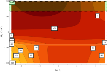
In Fig. 7, the variation of $\Delta_{+}$ in the $M_{\lambda}-\tan\theta_{\lambda}$ plane is shown. We take $M_{1}=600$ GeV and $\tan\beta=10$ with $\mu=M_{2}=250\ {\rm GeV}$. We do not vary $M_{\lambda}$ beyond $\pm 200\ {\rm GeV}$, since even at this value $\lambda$ already exceeds 1. The Figure clearly shows that we get the largest (negative) splitting when $M_{\lambda}$ is positive and $\tan\theta_{\lambda}$ is negative, up to $\Delta_{+}\sim-\mathcal{O}(50\ {\rm GeV})$. The shaded area above the dashed line is excluded since it results in a chargino with mass $m_{\tilde{\chi}^{\pm}_{1}}<101$ GeV. If $\mu=M_{2}$ is reduced, $\Delta_{+}$ becomes larger (negative). On the other hand, the upper bound on $M_{\lambda}$ from the bound on the chargino mass also decreases rapidly. For larger values of $\mu=M_{2}$, the upper bound on $M_{\lambda}$ increases and effectively one can also find a larger splitting.

From various analytical results and numerical figures it is clear that a chargino can be significantly lighter than the lightest neutralino. The mass difference can far exceed the size of radiative corrections to the gaugino masses.

• •

  The expressions for the mass differences between the lightest neutralino and the lightest chargino in Eq. (12) and in Eq. (13) were obtained for $\tan\beta>1$. The case $\tan\beta<1$ can be obtained by substituting $\sin\beta\leftrightarrow\cos\beta$.

• •

  The expressions for $\Delta_{+}$ are given in Eq. (14) and in Eq. (15) when $\mu_{d}$ is large. An alternate limit where $\mu_{u}$ is greater than all other relevant masses may be found by substituting $\sin\beta\leftrightarrow\cos\beta$ in Eq. (14) and in Eq. (15).

• •

  Given the results from the various limits, combined with Figs. 6 and 6, we find that at $\tan\beta=1$, a neutralino is always the lightest gaugino.

• •

  Finally, in the absence of $\lambda$ couplings, the mass difference $\Delta_{+}$ can be obtained in the Higgsino limit without decoupling $M_{1}$. Starting with Eqs. (12) and (14), hold $\tan\theta_{\lambda}$ finite, while independently taking $M_{\lambda}\rightarrow 0$. We obtain

  $$\begin{split}\mu_{u}=\mu_{d}=\mu\quad&\rightarrow\quad\Delta_{+}=-\;\mu\;M_{W}^{2}\left(\frac{2\sin^{2}\beta-1}{M_{2}^{2}}-\frac{\tan^{2}\theta_{W}}{M_{1}^{2}}\right)\;,\\ \text{Large }\mu_{d}\quad&\rightarrow\quad\Delta_{+}=-\;\sin^{2}\beta\;\mu\;M_{W}^{2}\left(\frac{1}{M_{2}^{2}}-\frac{\tan^{2}\theta_{W}}{M_{1}^{2}}\right)\;.\end{split}$$

  (16)

  These expressions demonstrate the chargino can be lighter than the neutralino in the MRSSM without $\lambda$ couplings.

We model the inclusive sparticle signal by the total production cross section for all twelve species of squarks. We do not consider the leptons or Higgses, and assume all squarks to be degenerate in mass. The inclusive squark production cross section as a function of the common squark mass is shown in Fig. 12 below.

In this scenario, the squarks first decay into a quark plus chargino or neutralino. The subsequent decays of the heavy (non-NLSP) charginos/neutralinos depend on the details of the gaugino spectrum: if kinematically allowed, heavy gauginos decay to a light gaugino plus a gauge bosons, otherwise they will decay into three-body decay final state containing a light gauginos plus two fermions. Finally, the chargino NLSPs each decay into $W$ + gravitino. Thus, every supersymmetric event contains at least two on-shell $W$s plus missing energy. Using this model for sparticle production, we want to discuss the sparticle discovery potential via excesses in $W^{+}W^{-}+\hbox to0.0pt{\hbox to7.95831pt{\hfil/\hfil}\hss}E_{T}+X$. Some possible decay chains are shown in Fig. 13.

where $\tilde{\chi}^{+}_{2},\tilde{\chi}^{0}$ are the second-lightest chargino and lightest neutralino respectively. As we can see, in addition to on-shell $W$ pairs, inclusive sparticle events involve cascades containing additional (hard) quarks and leptons. These extra leptons/jets are especially important in scenarios where the chargino lives longer than $\sim 25\ {\rm ns}$: by the time the long-lived charginos decay to objects which can be triggered on, the next bunch-crossing will have occurred in the detector, causing the charginos to be associated with the wrong event. However, if there are extra leptons/jets present in the sparticle decays, one can trigger on those objects instead of on the chargino decay products. Then, by refining the analysis offline to search for charged tracks, the presence of charginos could be revealed.

Another complication in this scenario is the possibility that the second-heaviest chargino and/or the lightest neutralino decay directly into gravitino + $X$ rather than decay via three-body decays. If the heavier chargino decays directly, the signal will still contain two $W$ bosons plus a pair a gravitinos, while if a neutralino decays directly one of the $W$s is replaced by a hard photon or $Z$ ¹¹ 1 Neutral Higgses are also a possibility, which we ignore for simplicity here.. The effect of the direct gravitino decays depends on the relative rates:

where $\Delta$ is the mass difference between the heavy chargino/neutralino ($\tilde{\chi}_{H}$) and the NLSP ($\tilde{\chi}_{L}$): $\Delta=m_{\tilde{\chi}_{H}}-m_{\tilde{\chi}_{L}}$. The prefactor $N_{f}$ is the number of fermionic degrees of freedom $\tilde{\chi_{L}}$ is kinematically allowed to decay into, and $\xi_{L},\xi_{R},(\kappa)$ are mixing angles from the chargino-neutralino-$X$ ($\tilde{\chi}_{H}$-gravitino-$X$) interactions; values in the limits of interest are given in Table 2. We plot $R_{\Gamma}$ for the neutralino as a function of the mass splitting $\Delta$ and gravitino mass in Fig. 14 below.

The region where direct decays are important is restricted to light gravitinos and small splittings. For gravitinos heavier than a few tenths of an eV, the three body decays are always dominant in either of the MRSSM limits we consider. For the MSSM, the large bino component of the lightest neutralino leads to a large $\kappa_{\gamma\tilde{G}}$ and suppressed $\xi_{L,R}$, thus direct decays can be important for gravitinos as heavy as $1\ {\rm eV}$. Neglecting direct decays of heavy gauginos to gravitinos, we now explore various search strategies and backgrounds to $W^{+}W^{-}+\hbox to0.0pt{\hbox to7.95831pt{\hfil/\hfil}\hss}E_{T}$.

The experimental search strategy will depend greatly on the lifetime of the chargino. If the chargino is long-lived but decays within the detector, it will leave a charged track, possibly leading to a displaced vertex. As mentioned above, triggering on the long-lived charginos is troublesome. However, provided they can be found, displaced vertices are great discriminant of new physics from background ²² 2 Lifetimes in the vicinity of $5$ ns would actually be ideal: $5\ {\rm ns}$ is small enough that triggering/resolution is not an issue, yet long enough that timing information in the calorimeter could be used to differentiate signal from background. We thank Dirk Zerwas for bringing this point to our attention..

If the charginos decay promptly, conventional variables such as $H_{T}=\sum_{i=\ell,j}p_{T}$ and $M_{eff}=H_{T}+\hbox to0.0pt{\hbox to7.95831pt{\hfil/\hfil}\hss}E_{T}$ [39] will likely be the first to indicate discovery. Additionally, these variables will be effective handles for separating signal from background. The optimum value for cuts in these variables depends on the superpartner mass scale.

In the case of prompt charginos, the dominant SM backgrounds in $W^{+}W^{-}\hbox to0.0pt{\hbox to7.95831pt{\hfil/\hfil}\hss}E_{T}+X$ are: $\bar{t}t+{\rm jets\ }$, single top + jets, $W^{+}W^{-}/W^{\pm}Z+{\rm jets}$, and $W^{\pm}/Z+{\rm jets}$ ³³ 3 By “+jets” we are including heavy quark flavors $(b,c)$ as well as light.. Exactly which background is most important will depend on the strategy for $W$ pair detection.

Irreducible SM backgrounds that result from $W^{+}W^{-}\rightarrow\ell+\nu+jj$, contain only one true source of missing energy - the neutrino from the leptonic $W$ decay. In addition to providing less $\hbox to0.0pt{\hbox to7.95831pt{\hfil/\hfil}\hss}E_{T}$ to SM events (compared to two neutrinos), with a single source of missing energy one can reconstruct the transverse mass of the $W$ ($m_{T,W}$) from the $p_{T}$ of the lepton and the $\hbox to0.0pt{\hbox to7.95831pt{\hfil/\hfil}\hss}E_{T}$. For the SM events the transverse mass distribution will exhibit a peak near $M_{W}$, followed by steep dropoff. Meanwhile, the $m_{T}$ distribution for the signal will fall much slower (after $M_{W}$) due to the excess $\hbox to0.0pt{\hbox to7.95831pt{\hfil/\hfil}\hss}E_{T}$ carried by the gravitinos. Therefore, by cutting on $m_{T,W}\gtrsim 100\ {\rm GeV}$ we can remove a large fraction of the background while maintaining the signal. The signal may still be polluted by events where two leptons are produced but one of them is missed by the detector. An important background which falls into this category is $\bar{t}t\rightarrow\ell\nu\ell^{\prime}\nu^{\prime}\bar{b}b$ ⁴⁴ 4 The $\bar{t}t$ and single-top backgrounds can be reduced further by rejecting any events with a $b$-tag, at the expense of compromising the stop/sbottom contribution to $(\ref{fig:squarkprod})$, while $W/Z+{\rm jets}$ can be reduced by requiring two jets to reconstruct a $W$..

A second channel to search for $W$ pairs, $\ell\nu\ell^{\prime}\nu^{\prime}$, has the advantage of an additional lepton, which greatly reduces the $W^{\pm}/Z~+$ jets background. Unfortunately, when both $W$’s decay leptonically, the SM backgrounds have higher missing energy, so the efficiency of $\hbox to0.0pt{\hbox to7.95831pt{\hfil/\hfil}\hss}E_{T}$ cuts will be reduced. The $p_{T}$ and $\eta$ of the two leptons remain useful variables for discriminating signal from background.

The third possibility is for both $W$s to decay hadronically. In that case, the signal is 4+ jets + $\hbox to0.0pt{\hbox to7.95831pt{\hfil/\hfil}\hss}E_{T}$ , with four of the jets breaking up into two pairs, each pair reconstructing to a $W$. Although reconstructing $W$s can be difficult with realistic jet resolution, the background can be greatly suppressed by imposing hard cuts ($100\ {\rm GeV}$ or more) on the $p_{T}$ of the reconstructed $W$s and the missing energy. However, unless there is an additional lepton in these events from an earlier cascade decay, multijet QCD becomes an important and difficult background. Further detailed study, in all of the channels mentioned above as well as for a more diverse spectrum are needed.

If the chargino NLSP is long-lived, a charged track will be visible in the detector. Depending on the exact lifetime of the chargino, the charged track will either exit the detector or end in a displaced vertex. Either way, a visible track allows us to rule out the majority of neutralino NLSP scenarios. However, distinguishing a chargino NLSP from a charged slepton NLSP requires more careful study.

As sleptons are much heavier their decay products, the lepton coming from the displaced vertex will tend to be collinear with the slepton track. On the other hand, because $W$s are so massive they will emerge from chargino decays without significant boosting; therefore chargino tracks will demonstrate a distinct kink feature. Additionally, $W$ bosons decay to jets and (democratically) into all three leptons - therefore chargino decays will lead to $e,\mu,\tau$ each in equal amounts, up to reconstruction and detector efficiency effects. Selectron and smuon NLSPs also decay to lepton plus $\hbox to0.0pt{\hbox to7.95831pt{\hfil/\hfil}\hss}E_{T}$, but their final state is a particular lepton flavor (for at least approximately flavor-diagonal slepton masses). By simply counting the number and type of leptons in a data sample, one should easily be able to distinguish selectrons/smuons from charginos. Stau NLSPs are somewhat trickier because taus decay democratically to electrons and muons; however, provided adequate tau-tagging capability at the LHC, staus should also be easily distinguishable from charginos.

Short-lived charginos are somewhat trickier. In principle, the identity of the particle produced along with the gravitino can tell us something about the NLSP; for neutralinos this spectator particle is likely a photon, for a chargino it will be a $W$, and for sleptons the spectator is a lepton. Additionally, the maximum energy achieved by the spectator depends on the LSP mass, allowing one to distinguish WIMP LSP scenarios from gravitino LSP scenarios [4]. In practice, the success of spectator-identification will depend on the details of the sparticle spectrum, and it is easy to dream up tricky scenarios.

To distinguish the chargino NLSP limit of the (N)MSSM from the MRSSM additional observables are needed. One handle is that the hallmark same-sign-lepton signal will be absent [24] whenever the gauginos have a Dirac mass. A second, though less robust discriminant is the mass difference between the lightest neutralino and the lightest chargino. In the MSSM the NLSP chargino occurs when several gauginos are nearly degenerate, thus it is difficult to arrange mass differences (even with large radiative corrections) greater than $\sim 10\ {\rm GeV}$. In the MRSSM large neutralino-chargino mass differences are easier to accommodate, especially if $\lambda,\lambda^{\prime}\neq 0$.

References

- [1] G. F. Giudice and R. Rattazzi, Phys. Rept. 322 (1999) 419–499, [hep-ph/9801271].
- [2] S. Ambrosanio, G. D. Kribs, and S. P. Martin, Nucl. Phys. B516 (1998) 55–69, [hep-ph/9710217].
- [3] N. Cabibbo, G. R. Farrar and L. Maiani, Phys. Lett. B 105, 155 (1981).
- [4] S. Dimopoulos, M. Dine, S. Raby, and S. D. Thomas, Phys. Rev. Lett. 76 (1996) 3494–3497, [hep-ph/9601367].
- [5] S. Ambrosanio, G. L. Kane, G. D. Kribs, S. P. Martin, and S. Mrenna, Phys. Rev. D54 (1996) 5395–5411, [hep-ph/9605398].
- [6] S. Dimopoulos, S. D. Thomas and J. D. Wells, Nucl. Phys. B 488, 39 (1997) [hep-ph/9609434].
- [7] J. A. Bagger, K. T. Matchev, D. M. Pierce and R. j. Zhang, Phys. Rev. D 55, 3188 (1997) [hep-ph/9609444].
- [8] S. Ambrosanio, G. D. Kribs, and S. P. Martin, Phys. Rev. D56 (1997) 1761–1777, [hep-ph/9703211].
- [9] S. Raby, Phys. Lett. B422 (1998) 158–162, [hep-ph/9712254].
- [10] Particle Data Group Collaboration, W. M. Yao et al., J. Phys. G33 (2006) 1–1232.
- [11] L. Randall and R. Sundrum, Nucl. Phys. B557 (1999) 79–118, [hep-th/9810155].
- [12] G. F. Giudice, M. A. Luty, H. Murayama, and R. Rattazzi, JHEP 12 (1998) 027, [hep-ph/9810442].
- [13] H.-C. Cheng, B. A. Dobrescu, and K. T. Matchev, Nucl. Phys. B543 (1999) 47–72, [hep-ph/9811316].
- [14] J. L. Feng, T. Moroi, L. Randall, M. Strassler, and S.-f. Su, Phys. Rev. Lett. 83 (1999) 1731–1734, [hep-ph/9904250].
- [15] G. F. Giudice and A. Pomarol, Phys. Lett. B372 (1996) 253–258, [hep-ph/9512337].
- [16] M. Drees, M. M. Nojiri, D. P. Roy, and Y. Yamada, Phys. Rev. D56 (1997) 276–290, [hep-ph/9701219].
- [17] D. M. Pierce, J. A. Bagger, K. T. Matchev, and R.-j. Zhang, Nucl. Phys. B491 (1997) 3–67, [hep-ph/9606211].
- [18] We have also found that the chargino can be the NLSP at tree-level when . In this region we find the mass difference is smaller than 1% of the NLSP mass. It is not obvious that this region remains after radiative corrections are taken into account, and thus we do not consider this region further.
- [19] P. Fayet, Phys. Lett. B78 (1978) 417.
- [20] J. Polchinski and L. Susskind, Phys. Rev. D26 (1982) 3661.
- [21] L. J. Hall and L. Randall, Nucl. Phys. B352 (1991) 289–308.
- [22] P. J. Fox, A. E. Nelson, and N. Weiner, JHEP 08 (2002) 035, [hep-ph/0206096].
- [23] A. E. Nelson, N. Rius, V. Sanz, and M. Unsal, JHEP 08 (2002) 039, [hep-ph/0206102].
- [24] Z. Chacko, P. J. Fox, and H. Murayama, Nucl. Phys. B706 (2005) 53–70, [hep-ph/0406142].
- [25] L. M. Carpenter, P. J. Fox, and D. E. Kaplan, [hep-ph/0503093].
- [26] I. Antoniadis, K. Benakli, A. Delgado, and M. Quiros, [hep-ph/0610265].
- [27] J. Hisano, M. Nagai, T. Naganawa, and M. Senami, Phys. Lett. B644 (2007) 256–264, [hep-ph/0610383].
- [28] K. Hsieh, Phys. Rev. D77 (2008) 015004, [0708.3970].
- [29] G. D. Kribs, E. Poppitz, and N. Weiner, [0712.2039].
- [30] A. E. Blechman and S.-P. Ng, [0803.3811].
- [31] K. Intriligator, N. Seiberg, and D. Shih, JHEP 04 (2006) 021, [hep-th/0602239].
- [32] J. Bagger, E. Poppitz, and L. Randall, Nucl. Phys. B426 (1994) 3–18, [hep-ph/9405345].
- [33] V. D. Barger, M. S. Berger, and P. Ohmann, Phys. Rev. D49 (1994) 4908–4930, [hep-ph/9311269].
- [34] M. Pospelov and A. Ritz, Annals Phys. 318 (2005) 119–169, [hep-ph/0504231].
- [35] B. C. Allanach, A. Djouadi, J. L. Kneur, W. Porod, and P. Slavich, JHEP 09 (2004) 044, [hep-ph/0406166].
- [36] A. G. Cohen, T. S. Roy, and M. Schmaltz, JHEP 02 (2007) 027, [hep-ph/0612100].
- [37] T. S. Roy and M. Schmaltz, Phys. Rev. D77 (2008) 095008, [0708.3593].
- [38] H. Murayama, Y. Nomura, and D. Poland, Phys. Rev. D77 (2008) 015005, [0709.0775].
- [39] I. Hinchliffe, F. E. Paige, M. D. Shapiro, J. Soderqvist, and W. Yao, Phys. Rev. D55 (1997) 5520–5540, [hep-ph/9610544].