Galaxy Clustering & Galaxy-Galaxy Lensing:
A Promising Union to Constrain Cosmological Parameters
Abstract
Galaxy clustering and galaxy-galaxy lensing probe the connection between galaxies and their dark matter haloes in complementary ways. Since the clustering of dark matter haloes depends on cosmology, the halo occupation statistics inferred from the observed clustering properties of galaxies are degenerate with the adopted cosmology. Consequently, different cosmologies imply different mass-to-light ratios for dark matter haloes. Galaxy-galaxy lensing, which yields direct constraints on the actual mass-to-light ratios, can therefore be used to break this degeneracy, and thus to constrain cosmological parameters. In this paper we establish the link between galaxy luminosity and dark matter halo mass using the conditional luminosity function (CLF), , which gives the number of galaxies with luminosities in the range that reside in a halo of mass . We constrain the CLF parameters using the galaxy luminosity function and the luminosity dependence of the correlation lengths of galaxies. The resulting CLF models are used to predict the galaxy-galaxy lensing signal. For a cosmology that agrees with constraints from the cosmic microwave background, i.e. , the model accurately fits the galaxy-galaxy lensing data obtained from the SDSS. For a comparison cosmology with , however, we can accurately fit the luminosity function and clustering properties of the galaxy population, but the model predicts mass-to-light ratios that are too high, resulting in a strong overprediction of the galaxy-galaxy lensing signal. We conclude that the combination of galaxy clustering and galaxy-galaxy lensing is a powerful probe of the galaxy-dark matter connection, with the potential to yield tight constraints on cosmological parameters. Since this method mainly probes the mass distribution on relatively small (non-linear) scales, it is complementary to constraints obtained from the galaxy power-spectrum, which mainly probes the large-scale (linear) matter distribution.
Keywords:
galaxies: halos — large-scale structure of Universe — dark matter — cosmological parameters — gravitational lensing — methods: statistical1 Introduction
With the advent of large galaxy redshift surveys, it has become possible to obtain accurate measurements of the clustering of galaxies as a function of their properties, such as luminosity, morphology and color (e.g. Guzzo et al. 2000; Norberg et al. 2001, 2002; Zehavi et al. 2005; Wang et al. 2007). Since galaxies are believed to form and reside in dark matter haloes, the clustering strength of a given population of galaxies can be compared to that of dark matter haloes as predicted by numerical simulations or the extended Press-Schechter formalism. Such a comparison reveals a wealth of information about the so-called galaxy-dark matter connection (e.g. Jing, Mo & Börner 1998; Peacock & Smith 2000; Berlind & Weinberg 2002; Yang, Mo & van den Bosch 2003; van den Bosch, Yang & Mo 2003; van den Bosch et al. 2007).
Unfortunately, this method of constraining the link between galaxies and dark matter haloes using galaxy clustering has one important shortcoming: the halo occupation statistics inferred from the observed clustering properties depend on the cosmological parameters adopted. More precisely, models based on different cosmologies can fit the clustering data equally well by simply relying on different halo occupation statistics or, equivalently, different mass-to-light ratios. In order to break this degeneracy between cosmology and halo occupation statistics independent constraints on the mass-to-light ratios are required (e.g. van den Bosch, Mo & Yang 2003; Tinker et al. 2005). One method that can provide these constraints is galaxy-galaxy lensing (hereafter g-g lensing), which probes the mass distributions (and hence the halo masses) around galaxies. This implies that the combination of clustering and lensing in principle holds the potential to put constraints on cosmological parameters (Seljak et al. 2005; Yoo et al. 2006).
The first attempt to detect g-g lensing was made by Tyson et al. (1984), but because of the relatively poor quality of their data they were unable to detect a statistically significant signal. With the advent of wider and deeper surveys becoming available, however, g-g lensing has now been detected with very high significance, and as function of various properties of the lensing galaxies (e.g. Griffiths et al. 1996; Hudson et al. 1998; McKay et al. 2001; Guzik & Seljak 2002; Hoekstra et al. 2003, 2004; Sheldon et al. 2004, 2007a,b; Mandelbaum et al. 2006; Heymans et al. 2006; Johnston et al. 2007; Parker et al. 2007; Mandelbaum, Seljak & Hirata 2008). Unfortunately, a proper interpretation of these data in terms of the link between galaxies and dark matter haloes has been hampered by the fact that the lensing signal can typically only be detected when stacking the signal of many lenses. Since not all lenses reside in haloes of the same mass, the resulting signal is a non-trivial average of the lensing signal due to haloes of different masses. Most studies to date have assumed that the relation between the luminosity of a lens galaxy and the mass of its halo is given by a simple power-law relation with zero scatter (see Limousin et al. 2007 for a detailed overview). However, it has become clear, recently, that the scatter in this relation between light and mass can be very substantial (More et al. 2008b, and references therein). As shown by Tasitsiomi et al. (2004), this scatter has a very significant impact on the actual lensing signal, and thus has to be accounted for in the analysis. In addition, central galaxies (those residing at the center of a dark matter halo) and satellite galaxies (those orbiting around a central galaxy) contribute very different lensing signals, even when they reside in haloes of the same mass (e.g. Natarajan, Kneib & Smail 2002; Yang et al. 2006; Limousin et al. 2007). This has to be properly accounted for (see e.g. Guzik & Seljak 2002), and requires knowledge of both the satellite fractions and of the spatial number density distribution of satellite galaxies within their dark matter haloes.
Over the years, numerous techniques have been developed to interpret galaxy-galaxy lensing measurements (Schneider & Rix 1997; Natarajan & Kneib 1997; Brainerd & Wright 2002; Guzik & Seljak 2001). Several authors have also used numerical simulations to investigate the link between g-g lensing and the galaxy-dark matter connnection (e.g., Tasitsiomi et al. 2004; Limousin et al. 2005; Natarajan, De Lucia & Springel 2007; Hayashi & White 2007). It has become clear from these studies that g-g lensing in principle contains a wealth of information regarding the mass distributions around galaxies; in addition to simply probing halo masses, g-g lensing also holds the potential to measure the shapes, concentrations and radii of dark matter haloes, and the first observational results along these lines have already been obtained (Natarajan et al. 2002; Hoekstra et al. 2004; Mandelbaum et al. 2006; Limousin et al. 2007; Mandelbaum et al. 2008).
In this paper we use an analytical model, similar to that developed by Seljak (2000) and Guzik & Seljak (2001), to predict the g-g lensing signal as a function of the luminosity of the lenses starting from a model for the halo occupation statistics that is constrained to fit the abundances and clustering properties of the lens galaxies. A comparison of these predictions with the data thus allows us to test the mass-to-light ratios inferred from the halo occupation model, and ultimately to constrain cosmological parameters. The model assumes that haloes have NFW (Navarro, Frenk & White 1997) density distributions, and that satellite galaxies follow a radial number density distribution that is unbiased with respect to the dark matter. The occupation statistics are described via the conditional luminosity function (CLF; see Yang et al. 2003), which specifies the average number of galaxies of given luminosity that reside in a halo of given mass. This CLF is ideally suited to model g-g lensing, as it allows one to properly account for the scatter in the relation between luminosity and halo mass, and to split the galaxy population in centrals and satellites. We demonstrate how these different galaxy populations contribute to the lensing signal in different luminosity bins, and show that uncertainties related to the expected concentrations of dark matter haloes and the radial number density distributions of satellite galaxies do not have a significant impact on our results.
Assuming a flat CDM cosmology with parameters supported by the third year data release of the Wilkinson Microwave Anisotropy Probe (WMAP, see Spergel et al. 2007), we obtain a CLF that accurately fits the abundances and clustering properties of SDSS galaxies. Using our analytical model, we show that this same CLF also accurately matches the g-g lensing data obtained from the SDSS by Seljak et al. (2005) and Mandelbaum et al. (2006) without any additional tuning of the model parameters. However, if we repeat the same exercise for a cosmology with a matter density and power-spectrum normalization that are slightly ( 20 percent) higher, the model that fits the clustering data can no longer simultaneously fit the g-g lensing data. This confirms that a joint analysis of clustering and g-g lensing is an extremely promising method to constrain cosmological parameters. In a companion paper (Li et al. 2008), we use the SDSS galaxy group catalogue of Yang et al. (2007) to predict the g-g lensing signal, which we compare to data from the SDSS. Although, Li et al. obtain their halo occupation statistics from a galaxy group catalogue, rather than from the galaxy clustering properties, they obtain very similar results.
The present paper is organized as follows. We review the necessary formalism of g-g lensing in § 2, with a detailed description of the model used to interpret the g-g lensing signal. The CLF, used to describe the connection between galaxies and dark matter haloes, is introduced in § 3. The properties of the predicted g-g lensing signal are illustrated in § 4 together with a comparison between theoretical predictions and SDSS data. A detailed analysis of the assumptions entering the model is presented in § 5. Conclusions are presented in § 6.
2 The Halo-Model Description of Galaxy-Galaxy Lensing
Galaxy-galaxy lensing measures the tangential shear distortions, , in the shapes of background galaxies (hereafter sources) induced by the mass distribution around foreground galaxies (hereafter lenses). Since the tangential shear distortions due to a typical lens galaxy (and its associated dark matter halo) are extremely small, and since background sources have non-zero intrinsic ellipticities, measuring with sufficient signal-to-noise requires large numbers of background galaxies. Except for extremely deep surveys behind clusters of galaxies, which have a large surface area, the number density of background sources is insufficient for a reliable measurement of around individual lenses. In practice, this problem can be circumvented by stacking many lenses according to some observable property. For example, Mandelbaum et al. (2006) measured as a function of the transverse comoving distance by stacking thousands of lenses in a given luminosity bin . The resulting shear holds information regarding the characteristic mass of the haloes that host galaxies with luminosity , and hence can be used to constrain the galaxy-dark matter connection.
The tangential shear as a function of the projected radius around the lenses is related to the excess surface density (ESD) profile, , according to
| (1) |
where is the projected surface density and is its average inside ,
| (2) |
(Miralda-Escudé 1991; Sheldon et al. 2004). The so-called critical surface density, , is a geometrical parameter given by
| (3) |
with , and the comoving distances to the source, the lens and between the two, respectively, and with the redshift of the lens.
The projected surface density is related to the galaxy-dark matter cross correlation, , according to
| (4) |
where is the average density of matter in the Universe and the integral is along the line of sight with the comoving distance from the observer. The three-dimensional comoving distance is related to through (see Fig. 1 for an illustration of the geometry).

Since goes to zero in the limit , and since in practice is small, we can approximate Eq. (4) using
| (5) |
which is the expression we adopt throughout.
The main goal of this paper is to test the halo occupation statistics inferred from galaxy clustering data with g-g lensing data. As is evident from the above equations, the lensing signal is completely specified by the galaxy dark matter cross correlation, which, as we demonstrate below, can be computed from a given halo occupation model. For computational convenience, we will be working in Fourier space, where the related quantity is the galaxy-dark matter cross power spectrum
| (6) |
In order to compute this power spectrum, we follow Seljak (2000) and Guzik & Seljak (2001), and adopt the halo model, according to which all dark matter is partitioned over dark matter haloes (see also Mandelbaum et al. 2005a). As usual in the halo model, it is convenient to split into two terms; a 1-halo term, which describes the cross correlation between galaxies and the dark matter particles that reside in the same halo, and a 2-halo term, where each galaxy is cross correlated with the dark matter in all haloes except for the one that hosts the galaxy in question. The computation of these two terms has to account for two important complications. First of all, because of the stacking procedure used in order to achieve sufficient signal-to-noise, the ESD contains signal from haloes with different masses. A proper estimate of , therefore, requires the full probability distribution that a galaxy with the stacking property used (in this case luminosity) resides in a dark matter halo of mass . Secondly, central galaxies (those residing at the center of a dark matter halo) and satellite galaxies (those orbiting around a central galaxy) contribute very different lensing signals, even when they reside in haloes of the same mass (e.g., Yang et al. 2006). This has to be properly accounted for, and requires knowledge of both the satellite fractions and of the spatial number density distribution of satellite galaxies within their dark matter haloes. Based on these considerations, we split in four terms:
| (7) | |||||
where ‘c’ and ‘s’ stand for ‘central’ and ‘satellite’, respectively. The reason for explicitely writing the central and satellite fractions ( and , respectively) in the above equation will become apparent below, in which we describe each of these four terms in turn.
2.1 The 1-halo term
The one-halo central term of the power spectrum describes the dark matter distribution inside haloes hosting central galaxies. For a single, central lensing galaxy, it simply reflects the Fourier transform of the overdensity of the dark matter halo in which the lens resides:
| (8) |
where is the normalized Fourier transform of the mass density profile, :
| (9) |
with the radius of the halo (see §2.3 below). However, because the lensing signal is measured by stacking galaxies with luminosities in the range , we have that
| (10) |
where is the probability that a central galaxy with luminosity resides in a halo of mass . This probability function reflects the halo occupation statistics, and, using Bayes’ theorem, can be written as
| (11) |
Here is the average number of central galaxies with luminosities in the range that reside in a halo of mass , is the halo mass function and
| (12) |
is the comoving number density of central galaxies in the given luminosity range.
Combining (10) and (11), the first term of the galaxy-dark matter power spectrum can be written as
| (13) |
where is the total number density of all galaxies (centrals plus satellites) with luminosities in the range . Note that, for brevity, we don’t explicitely write the luminosity dependence of and , but it is understood that and .
The 1-halo satellite term is similar to the 1-halo central term, except for the fact that satellite galaxies do not reside at the center of their dark matter halo, but follow a number density distribution . Consequently, the 1-halo lensing signal due to satellite galaxies involves a convolution of with the mass density profile of the host halo in which they reside. Using that in Fourier space a convolution corresponds to a simple multiplication, we obtain:
| (14) |
with
| (15) |
the Fourier transform of normalized by which is the average number of satellites with that reside in a halo of mass . We assume that there is no luminosity segregation amongst the satellites, so that they all follow the same radial profile, independent of their luminosity. We write the probability that a satellite galaxy with resides in a halo of mass as
| (16) |
with
| (17) |
the comoving number density of satellite galaxies with luminosities in the range . The 1-halo satellite term can thus be written as
| (18) |
where we have used that . Note that .
2.2 The 2-halo term
The 2-halo term of the power spectrum describes the correlation between galaxies and dark matter particles belonging to separate haloes. Within the halo model, this means cross correlating each galaxy with all the dark matter haloes other than the one in which the galaxy in question resides. Using the fact that dark matter haloes are a biased tracer of the dark matter mass distribution, the contribution to the 2-halo term due to central galaxies can be written as
| (19) |
where and are the non-linear power spectrum of the dark matter and the halo bias function, respectively. The first integral reflects the contribution of the central galaxies, while the second integral describes the dark matter density field partitioned over haloes. Using (11) we obtain
| (20) |
Similarly, the satellite part of the 2-halo term is given by
| (21) |
where the second integral now accounts for the number density distribution of satellite galaxies in haloes of mass .
Note that equations (20) and (21) ignore halo exclusion, i.e. the fact that, in the halo model, haloes can not overlap. In the Appendix, we present an approximate method to take halo exclusion into account. Far from being a detailed treatment, the suggested procedure accounts only for the most relevant effect, i.e. the exclusion of dark matter particles residing in the same host halo of central galaxies (see Appendix for further details). Unless stated otherwise, all the results shown throughout the paper are obtained applying halo exclusion as modelled in the Appendix.
In addition, a technical, as well as conceptual, issue arises in calculating the 2-halo terms introduced in equations (20) and (21). Let us rewrite these two equations in the following compact form:
| (22) |
where , and are
| (23) |
The evaluation of these integrals is somewhat tedious numerically, as it requires knowledge of the halo mass function and the halo bias function over the entire mass range . Since these have only been tested against numerical simulations over a limited range of halo masses (), it is also unclear how accurate they are. In practice, though, these problems can be circumvented as follows. First of all, because of the exponential cut-off in the halo mass function, it is sufficiently accurate to perform the integrations of Eq. (23) only up to . Secondly, and contain the halo occupation statistics, and , respectively, which, for all luminosities of interest in this paper, are equal to zero for . Therefore, and can be computed accurately by only integrating over the mass range . Unfortunately, the integrand of does not become negligibly small below a given halo mass. However, in this case we can use the approach introduced by Yoo et al. (2006): we write as the sum of two terms, , where:
| (24) |
Following Yoo et al. (2006), we use the fact that over the relevant range of as long as is sufficiently small. This allows us to write
| (25) | |||||
where the last equality follows from the fact that the distribution of matter is by definition unbiased with respect to itself. Detailed tests have shown that this procedure yields results that are sufficiently accurate as long as . Throughout we adopt .
2.3 Model Ingredients
The computation of the galaxy-dark matter cross correlation (or its power spectrum) as outlined in the previous subsections, requires the following ingredients:
- •
The halo mass function, , specifying the comoving number density of dark matter haloes of mass .
- •
The halo bias function, , which describes how haloes of mass are biased with respect to the overall dark matter distribution.
- •
The non-linear power spectrum of the dark matter distribution, .
- •
The mass density distribution of dark matter haloes, .
- •
The number density distribution of satellite galaxies in dark matter haloes, .
- •
The halo occupation statistics for central and satellite galaxies, as parameterized by and , respectively.
All these ingredients depend on cosmology. In this paper we consider two flat CDM cosmologies. The first has a matter density , a baryonic matter density , a Hubble parameter , a power-law initial power spectrum with spectral index and a normalization . These are the parameters that best-fit the 3-year data release of the Wilkinson Microwave Anisotropy Probe (WMAP, see Spergel et al. 2007), and we will refer to this set of cosmological parameters as the WMAP3 cosmology. The second cosmology has , , , and . With strong support from the first year data release of the WMAP mission (see Spergel et al. 2003), this choice of parameters has been considered in many previous studies. In what follows we will refer to this second set of parameters as the WMAP1 cosmology. For clarity, the parameters of both cosmologies are listed in Table 1.
| WMAP3 | ||||||
|---|---|---|---|---|---|---|
| WMAP1 |
We define dark matter haloes as spheres with an average overdensity of , with a mass given by
| (26) |
Here is the radius of the halo. We assume that dark matter haloes follow the NFW (Navarro, Frenk & White 1997) density distribution
| (27) |
where is a characteristic radius and is a dimensionless amplitude which can be expressed in terms of the halo concentration parameter as
| (28) |
Numerical simulations show that is correlated with halo mass, and we use the relations given by Macciò et al. (2007), converted to our definition of halo mass.
For the halo mass function, , and halo bias function, , we use the functional forms suggested by Warren et al. (2006) and Tinker et al. (2005), respectively, which have been shown to be in good agreement with numerical simulations. The linear power spectrum of density perturbations is computed using the transfer function of Eisenstein & Hu (1998), which properly accounts for the baryons, while the evolved, non-linear power spectrum of the dark matter, , is computed using the fitting formula of Smith et al. (2003).
For the number density distribution of the satellite galaxies, we assume a generalized NFW profile (e.g., van den Bosch et al. 2004):
| (29) |
which scales as and at small and large radii, respectively. Similar to the dark matter mass distribution, has an effective scale radius , and can be parameterized via the concentration parameter . Observations of the number density distribution of satellite galaxies in clusters and groups seem to suggest that is in good agreement with an NFW profile, for which (e.g., Beers & Tonry 1986; Carlberg, Yee & Ellingson 1997a; van der Marel et al. 2000; Lin, Mohr & Stanford 2004; van den Bosch et al. 2005a). Several studies have suggested, however, that the satellite galaxies are less centrally concentrated than the dark matter, corresponding to (e.g., Yang et al. 2005; Chen 2007; More et al. 2008b). For our fiducial model we adopt , for which (i.e., satellite galaxies follow the same number density distribution as the dark matter particles). In §5.3 we examine how the results depend on and .
The final ingredient is a model for the halo occupation statistics. In their attempt to model the g-g lensing signal obtained from the SDSS, Seljak et al. (2005) and Mandelbaum et al. (2006) made the oversimplified assumption of a deterministic relation between central galaxy luminosity and host halo mass. In particular, they used
| (30) |
where is the ‘characteristic’ mass of a halo that hosts a central galaxy with . However, a realistic relation between central galaxy luminosity and host halo mass will have some scatter. As demonstrated by Tasitsiomi et al. (2004), this scatter can have an important impact on the g-g lensing signal (see also §5.1 below). For the satellite galaxies, Seljak et al. (2005) and Mandelbaum et al. (2006) adopted a simple double power-law relation of the form
| (31) |
In this paper we improve upon the analysis by Seljak et al. (2005) and Mandelbaum et al. (2006) by using a more realistic model for the halo occupation statistics. Furthermore, rather than fitting the model to the lensing data, we constrain the occupation statistics using clustering data from the SDSS combined with a large galaxy group catalogue. Subsequently we use that model to predict the g-g lensing signal which we compare to g-g lensing data obtained from the SDSS.
As a final remark, we emphasise that different quantities, e.g. , , and , depend on redshift, , even though we have not made this explicit in the equations.
3 Conditional Luminosity Function
3.1 Model description
In order to specify the halo occupation statistics, we use the CLF, , which specifies the average number of galaxies with luminosities in the range that reside in a halo of mass (Yang, Mo & van den Bosch 2003; van den Bosch, Yang, Mo 2003). Following Cooray & Milosavljević (2005) and Cooray (2006), we write the CLF as
| (32) |
where and represent central and satellite galaxies, respectively. The occupation numbers required for the computation of the galaxy-dark matter cross correlation then simply follow from
| (33) |
where ‘x’ refers to either ‘c’ (centrals) or ‘s’ (satellites). Motivated by the results of Yang, Mo & van den Bosch (2008; hereafter YMB08), who analyzed the CLF obtained from the SDSS galaxy group catalogue of Yang et al. (2007), we assume the contribution from the central galaxies to be a log-normal:
| (34) |
Note that is the scatter in (of central galaxies) at a fixed halo mass. Moreover, is, by definition, the expectation value for the (10-based) logarithm of the luminosity of the central galaxy, i.e.,
| (35) |
For the contribution from the satellite galaxies we adopt a modified Schechter function:
| (36) |
which decreases faster than a Schechter function at the bright end. Note that , , , and are all functions of the halo mass . In the parametrization of these mass dependencies, we again are guided by the results of YMB08. In particular, for the luminosity of the central galaxies we adopt
| (37) |
so that for and for . Here is a characteristic mass scale, and is a normalization. Using the SDSS galaxy group catalogue, YMB08 found that to good approximation
| (38) |
and we adopt this parameterization throughout. For the faint-end slope and normalization of we adopt
| (39) |
and
| (40) |
with . This adds a total of six free parameters: , , , , and the characteristic halo mass . Neither of these functional forms has a physical motivation; they merely were found to adequately describe the results obtained by YMB08. Finally, for simplicity, and to limit the number of free parameters, we assume that is a constant. As shown in More et al. (2008b), this assumption is supported by the kinematics of satellite galaxies in the SDSS. Thus, altogether the CLF has a total of eleven free parameters.
| Sample | |||
|---|---|---|---|
| V1 | |||
| V2 | |||
| V3 | |||
| V4 | |||
| V5 | |||
| V6 |
Galaxy-galaxy clustering correlation lengths of Wang et al. (2007) used in this paper to constrain the CLF. Column (1) lists the ID of each volume limited sample, following the notation of Wang et al. (2007). Columns (2) and (3) indicate the absolute magnitude range and the mean redshift of each sample, while column (4) lists the correlation length plus its standard deviation (in ), obtained by fitting a power-law to the projected correlation function over the radial range . See Wang et al. (2007) for details.


Note that, with the parametrization of the CLF introduced above, the halo occupation statistics can be rewritten as:
| (41) |
where erf is the error function calculated at with and is the incomplete gamma function.
As shown in Yang et al. (2003) and van den Bosch et al. (2003), the CLF can be constrained using the observed luminosity function, , and the galaxy-galaxy correlation lengths as a function of luminosity, . Here we use the luminosity function (hereafter LF) of Blanton et al. (2003a) uniformly sampled at 41 magnitudes covering the range . Here indicates the -band magnitude KE corrected to following the procedure of Blanton et al. (2003b). For the correlation lengths as function of luminosity we use the results obtained by Wang et al. (2007) for six volume limited samples selected from the SDSS DR4. For completeness, these data are listed in Table 2. Finally, to strengthen our constraints, and to assure agreement with the CLF obtained from our SDSS group catalogue, we use the constraints on , and obtained by YMB08.
For a given set of model parameters, we compute the LF using
| (43) |
The galaxy-galaxy correlation function for galaxies with luminosities in the interval is computed using
| (44) |
Here is the non-linear correlation function of the dark matter, which is the Fourier transform of ,
| (45) |
is the radial scale dependence of the bias as obtained by Tinker et al. (2005), and is the bias of the galaxies, which is related to the CLF according to
| (46) |
with
| (47) | |||||
the average number of galaxies with luminosities in the range that reside in a halo of mass .
| Cosmology | ||||||||||||
|---|---|---|---|---|---|---|---|---|---|---|---|---|
| (1) | (2) | (3) | (4) | (5) | (6) | (7) | (8) | (9) | (10) | (11) | (12) | (13) |
| WMAP3 | 9.935 | 11.07 | 3.273 | 0.255 | 0.501 | 2.106 | 14.28 | -0.766 | 1.008 | -0.094 | 0.143 | 1.42 |
| WMAP1 | 9.915 | 11.16 | 3.336 | 0.248 | 0.484 | 2.888 | 14.54 | -0.854 | 0.906 | -0.062 | 0.140 | 1.70 |
The best-fit CLF parameters obtained from the MCMC analysis for the WMAP3 and WMAP1 cosmologies and the value of the corresponding reduced . Masses and luminosities are in and , respectively.
To determine the likelihood function of our free parameters we follow van den Bosch et al. (2007) and use the Monte-Carlo Markov Chain (hereafter MCMC) technique. The goodness-of-fit of each model is judged using with
| (48) |
| (49) |
and
| (50) | |||||
Here indicates an observed quantity and the subscripts ‘’, ‘’ and ‘GC’ refer to the luminosity function, the galaxy-galaxy correlation length and the group catalogue, respectively. Note that, by definition, . Table 4 lists the best-fit parameters obtained with the MCMC technique for both the WMAP1 and WMAP3 cosmologies, as well as the corresponding value of . Here is the number of degrees of freedom.
3.2 Results
Fig. 2 shows the results obtained for the WMAP3 cosmology. In each panel the blue contours indicate the 68 and 95 percent confidence levels obtained from the MCMC. The upper left-hand panel shows that the CLF model accurately fits the galaxy LF of Blanton et al. (2003a). The fit to the correlation lengths as function of luminosity, shown in the upper middle panel, is less accurate, although data and model typically agree at the level. The lower panels of Fig. 2 show the 68 and 95 percent confidence levels on , and , compared with the results obtained by YMB08 from the SDSS group catalogue of Y07. Since these data have been used as additional constraints, it should not come as a big surprise that the CLF is in good agreement with these data. We emphasise, though, that it is not trivial that a single halo occupation model can be found that can simultaneously fit the LF, the luminosity dependence of the galaxy-galaxy correlation functions, and the results obtained from a galaxy group catalogue.
Finally, the upper right-hand panel of Fig. 2 shows the satellite fraction,
| (51) |
as function of luminosity. This is found to decrease from at to virtually zero at . The fact that the satellite fraction decreases with increasing luminosity is in qualitative agreement with previous studies (Tinker et al. 2006; Mandelbaum et al. 2006; van den Bosch et al. 2007).
We have repeated the same exercise for the WMAP1 cosmology. As evident from Fig. 3, for this cosmology we can obtain a CLF that fits the data almost equally well (the reduced is only slightly higher than for the WMAP3 cosmology; see Table 3). Note that the group data (shown in the lower panels) differ from that in Fig. 2, even though the group catalogue is the same. This owes to the fact that the halo mass assignments of the groups are cosmology dependent (see Y07 for details). The satellite fractions inferred for this cosmology, shown in the upper right-hand panel of Fig. 3, are similar, though slightly higher, than for the WMAP3 cosmology, in excellent agreement with van den Bosch et al. (2007).
The fact that both cosmologies allow an (almost) equally good fit to these data, despite the relatively large differences in halo mass function and halo bias, illustrates that the abundance and clustering properties of galaxies allow a fair amount of freedom in cosmological parameters. However, as demonstrated in van den Bosch, Mo & Yang (2003), the best-fit CLFs for different cosmologies predict different mass-to-light ratios as function of halo mass. This is evident from Fig. 4, which shows the mass-to-light ratios as function of halo mass inferred from our CLF MCMCs for the WMAP1 and WMAP3 cosmologies. Here is the average, total luminosity of all galaxies with that reside in a halo of mass , which follows from the CLF according to
| (52) |
with the luminosity corresponding to a magnitude . Clearly, the mass-to-light ratios inferred for the WMAP1 cosmology are significantly higher than for the WMAP3 cosmology (see also van den Bosch et al. 2007, where a similar result was obtained using data from the 2dFGRS). Hence, the abundance and clustering properties of galaxies can be used to constrain cosmological parameters, as long as one has independent constraints on the mass-to-light ratios of dark matter haloes. This is exactly what is provided by g-g lensing. In the next section, we therefore use the CLF models presented here to predict the g-g lensing signal, which we compare to SDSS data.

4 Galaxy-Galaxy Lensing
4.1 Model Predictions
In order to compute the ESD, , as a function of the comoving separation on the sky, , we proceed as follows. We start by calculating the four different terms of the galaxy-dark matter cross power spectrum defined in § 2.1 and § 2.2. Next we inverse Fourier transform each of these terms using
| (53) |
where ‘’ stands for 1h or 2h, and ‘x’ refers to either ‘c’ (centrals) or ‘s’ (satellites). These are used to compute the corresponding four terms of the surface density, ,
| (54) |
Note that we are allowed to neglect the contribution coming from the constant background density, , (cf. equation [5]) because it will cancel in defining the ESD (this is known in gravitational lensing theory as the mass-sheet degeneracy). The final ESD then simply follows from
| (55) | |||||
in which the relative weight of each term is already included via the central and satellite fractions in the definitions of the corresponding power spectra11 1 Note that our notation differs slightly from that in Mandelbaum et al. (2006).


Before comparing the g-g lensing predictions from our CLF models to actual data, we first demonstrate how the four different terms contribute to the total ESD. The left-hand panel of Fig. 5 shows the obtained from our best-fit CLF model for the WMAP3 cosmology for three different luminosity bins, as indicated22 2 Here, for simplicity, we have used the halo mass function and halo bias function computed at . In §4.2, when we compare our models to data, we will use the halo mass function and halo bias function at the average redshift of the lenses instead.. Note that the fainter luminosity bins reveal a more ‘structured’ excess surface density profile, with a pronouced ‘bump’ at , which is absent in the of the brighter galaxies. The reason for this is evident from the middle and right-hand panels of Fig. 5, which show the contributions to from the four different terms for the faint () and bright () luminosity bins, respectively. In both cases, the 1-halo central term dominates on small scales. In the case of the faint galaxies, the 1-halo satellite term dominates over the radial range , and is responsible for the pronounced bump on intermediate scales. In the case of the bright bin, however, the 1-halo central term dominates all the way out to . This owes to the fact that bright centrals reside in more massive haloes, which are larger and cause a stronger lensing signal, and due to the fact that the satellite fraction of brighter galaxies is smaller. The fact that the 1-halo satellite term peaks at intermediate scales, rather than at , owes to the fact that reflects a convolution of the host halo mass density profile with the number density distribution of satellite galaxies. On large scales (), which roughly reflects two times the virial radius of the most massive dark matter haloes, the ESD is dominated by the 2-halo terms. Note that the faint galaxies, with , have the same large scale ESD as the bright galaxies with , indicating that they have similar values for their bias. This owes to the fact that many of the faint galaxies are satellites which reside in massive haloes. Note also that the 2-halo central term reveals a fairly abrupt truncation at small radii, which owes to halo-exclusion (see Appendix). This truncation also leaves a signature in the total lensing signal, which is more pronounced for the fainter lenses. We caution, however, that the sharpness of this feature is partially an artefact due to our approximate implementation of halo-exclusion. Nevertheless, it is clear from Fig. 5 that the excess surface densities obtained from g-g lensing measurements contain a wealth of information regarding the galaxy-dark matter connection.
4.2 Data
The g-g lensing data used here is described in Seljak et al. (2005) and Mandelbaum et al. (2006) and has been kindly provided to us by R. Mandelbaum. The catalogue of lenses consists of galaxies with magnitudes and redshifts taken from the main galaxy catalogue of the SDSS Data Release 4 (Adelman-McCarthy et al. 2006). This sample is split in 7 luminosity bins (see Table 4), and for each of these luminosity bins the excess surface density profiles, , have been determined from measurements of the shapes of more than 30 million galaxies in the SDSS imaging data down to an apparent -band magnitude of . The resulting data are shown as solid dots with errorbars in Fig. 6. We refer the reader to Mandelbaum et al. (2005b, 2006) for a detailed description of the data and of the methods used to determine the ESD profiles.
| ID | ||
|---|---|---|
| (1) | (2) | (3) |
| L1 | 0.032 | |
| L2 | 0.047 | |
| L3 | 0.071 | |
| L4 | 0.10 | |
| L5f | 0.14 | |
| L5b | 0.17 | |
| L6f | 0.20 |
Luminosity bins of the lenses. Column (1) lists the ID of each luminosity bin, following the notation of Mandelbaum et al. (2006). Column (2) indicates the magnitude range of each luminosity bin (all magnitudes are KE corrected to ). Column (3) indicates the mean redshift of the lenses in each luminosity bin. See Mandelbaum et al. (2006) for details.
4.3 Results for the WMAP3 Cosmology
Using the methodology outlined in §2 and §4.1, we now use the CLF for the WMAP3 cosmology obtained in §3 to predict the g-g lensing signal for the 7 luminosity bins listed in Table 4. For each luminosity bin we compute the ESD profile, , at the mean redshift of the sample, i.e., we use the halo mass function, , the halo bias function, , and the non-linear power spectrum, that correspond to the mean redshift listed in the third column of Table 4. We have verified, though, that computing simply at instead has a negligible impact on the results.
The results are shown in Fig. 6, where the solid dots with errorbars correspond to the SDSS data and the solid lines are the predictions of our best-fit CLF model (whose parameters are listed in Table 3). Note that this model fits the data remarkably well, which is quantified by the fact that the reduced is . We emphasize that there are no free parameters here: the ESD has been computed using the CLF that has been constrained using the LF and the clustering data. The good agreement between model and lensing data thus provides independent support for the halo occupation statistics described by our WMAP3 CLF model, in particular for the mass-to-light ratios and satellite fractions, which have an important impact on the lensing signal.
The different curves in each of the panels in Fig. 6 show the contribution to the lensing signal due to the four separate terms: (dotted lines), (short-dashed lines), (long-dashed lines), and (dot-dashed lines). In agreement with the examples shown in Fig. 5, the 1-halo central term becomes increasingly more dominant for more luminous lenses. In fact, in the brightest luminosity bin (L6f) it dominates over the entire radial range probed. In the low-luminosity bins, most of the observed lensing signal at is dominated by the 1-halo satellite term. The fact that our model accurately fits the data, thus supports the satellite fractions inferred from our CLF model, and shown in the upper right-hand panel of Fig. 2.
Both Seljak et al. (2005) and Mandelbaum et al. (2006) did not account for the contributions of the 2-halo terms in their analyses of the galaxy-galaxy lensing signal. Our model indicates that, although the 2-halo terms never dominate the total signal, they can contribute as much as 50 percent at large radii (). We thus conclude that the 2-halo terms cannot simply be ignored.
4.4 Comparison with the WMAP1 Cosmology
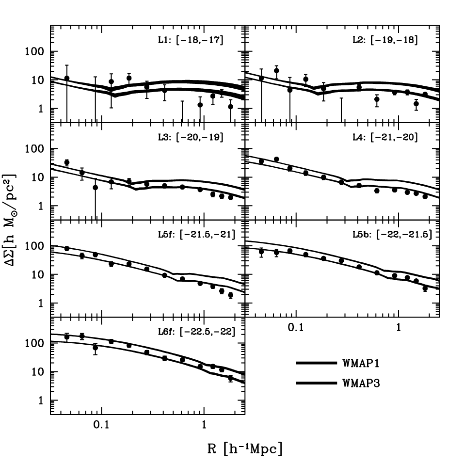
As shown in §3.2, the WMAP3 and WMAP1 cosmologies both allow a good fit to the clustering data, luminosity function and galaxy group results. However, the corresponding CLFs predict mass-to-light ratios that are significantly different. Since the galaxy-galaxy lensing signal is very sensitive to these mass-to-light ratios, it is to be expected that our WMAP3 and WMAP1 CLFs will predict significantly different ESD profiles, thus allowing us to discriminate between these two cosmologies.
Fig. 7 shows the 95 percent confidence levels for obtained from our CLF MCMCs for both the WMAP3 (blue) and WMAP1 (green) cosmologies. Indeed, as anticipated, for the WMAP1 cosmology we obtain excess surface densities that are significantly higher than for the WMAP3 cosmology, in accord with the higher mass-to-light ratios (cf. Fig. 4). A comparison with the SDSS data clearly favors the WMAP3 cosmology over the WMAP1 cosmology. In fact, for the latter our best-fit CLF model yields a reduced of , much larger than for the WMAP3 cosmology (). Note that the cosmological parameters for these two cosmologies are very similar: and differ only by percent (in addition to a percent difference in ). Yet, we can very significantly favor one cosmology over the other. This indicates that the combination of clustering data and g-g lensing data can be used to put tight constraints on cosmological parameters. A detailed analysis along these lines is deferred to a forthcoming paper (Cacciato et al. , in preparation).


5 Model Dependencies
Although our computation of the g-g lensing signal does not involve any free parameters (these are already constrained by the clustering data), a number of assumptions are made. In particular, haloes are assumed to be spherical and to follow a NFW density distribution, central galaxies are assumed to reside exactly at the center of their dark matter haloes, and satellite galaxies are assumed to follow a radial number density distribution that has the same shape as the dark matter mass distribution. In addition, we made assumptions regarding the functional form of the CLF. Although most of these simplifications are reasonable, and have support from independent studies, they may have a non-negligible impact on the predictions of the g-g lensing signal. If this is the case, they will affect the reliability of the cosmological constraints inferred from the data. In this section we therefore investigate how strongly our model predictions depend on these oversimplified assumptions.
Some of these dependencies were already investigated in our companion paper (Li et al. 2008). In particular, we have shown that the fact that realistic dark matter haloes are ellipsoidal, rather than spherical, can be safely ignored (i.e., its impact on the ESD profiles is completely negligible). On the other hand, if central galaxies are not located exactly at the center of their dark matter haloes, this may have a non-negligible impact on the lensing signal on small scales (). Fortunately, for realistic amplitudes of this offset (van den Bosch et al. 2005b), the effect is fairly small and only restricted to the most luminous galaxies (see Li et al. 2008 for details).
Below we investigate three additional model dependencies: the scatter in the relation between light and mass, the concentration of dark matter haloes, and the radial number density distribution of satellite galaxies. To that extent we compare our fiducial model (the best-fit CLF model for the WMAP3 cosmology presented above), to models in which we change only one parameter.
5.1 Scatter in the relation
An important improvement of our halo occupation model over that used by Seljak et al. (2005) and Mandelbaum et al. (2006) is that we allow for scatter in the relation between light and mass. In particular, we model the probability function as a log-normal with a scatter, , that is assumed to be independent of halo mass. As demonstrated in More et al. (2008b), this assumption is consistent with the kinematics of satellite galaxies, and it is supported by semi-analytical models for galaxy formation. Note, though, that this does not imply that the scatter in , which is the probability function which actually enters in the computation of the g-g lensing signal, is also constant. In fact, it is not. This is illustrated in Fig. 8, which shows of our fiducial model for four luminosity bins. Two trends are evident: more luminous centrals reside, on average, in more massive haloes, and they have a larger scatter in halo masses. As discussed in More, van den Bosch & Cacciato (2008), the fact that the scatter in increases with luminosity simply owes to the fact that the slope of becomes shallower with increasing (see the lower right-hand panels of Figs. 2 and 3). As is evident from Fig. 8, this is a strong effect, with the scatter in becoming extremely large at the bright end. Note that this scatter is not dominated by the width of the luminosity bin. Hence, even if one were able to use infinitesimally narrow luminosity bins when stacking lenses, the scatter in will still be very appreciable.
As first shown by Tasitsiomi et al. (2004), scatter in the relation between light and mass can have a very significant impact on the ESDs. This is demonstrated in the upper panels of Fig. 9, which show the impact on of changing by compared to our best-fit CLF value of ; all other parameters are kept fixed at their fiducial values (see Table 3). Note that these changes in have a negligible impact on for the low luminosity bins. At the bright end, however, relatively small changes in have a very significant impact on . In particular, increasing the amount of scatter reduces the ESD. This behavior owes to the shape of the halo mass function. Increasing the scatter adds both low mass and high mass haloes to the distribution, and the overall change in the average halo mass depends on the slope of the halo mass function. Brighter galaxies live on average in more massive haloes where the halo mass function is steeper. In particular, when the average halo mass is located at the exponential tail of the halo mass function, an increase in the scatter adds many more low mass haloes than massive haloes, causing a drastic shift in the average halo mass towards lower values. On the other hand, fainter galaxies live in less massive haloes, where the slope of the halo mass function is much shallower. Consequently, a change in the scatter does not cause a significant change in the average mass.
Clearly, if the g-g lensing signal is used to constrain cosmological parameters, it is important that one has accurate constraints on . From the clustering analysis presented in §3.2, we obtain (for both WMAP1 and WMAP3). This is in good agreement with previous studies: Cooray (2006), using a CLF to model the SDSS -band LF, obtained . YMB08, using a SDSS galaxy group catalogue, obtained , and More et al. (2008b), using the kinematics of satellite galaxies in the SDSS, find (all errors are 68% confidence levels). Although it is reassuring that very different methods obtain values that are in such good agreement, it is clear that the remaining uncertainty may have a weak impact on our ability to constrain cosmological parameters. Fortunately, the scatter only impacts the results at the bright end, so that one can always check the results by removing data from the brightest luminosity bins.
5.2 The dark matter halo concentration
The g-g lensing signal on small scales reflects the projected mass distribution of the haloes hosting the lensing galaxies. Therefore, the detailed shape of on small scales is sensitive to the mass distribution of dark matter haloes. In our model, we have assumed that dark matter haloes follow NFW profiles, which are characterized by their concentration parameters, . Halo concentrations are known to depend on both halo mass and cosmology, and various analytical models have been developed to describe these dependencies (Navarro et al. 1997; Bullock et al. 2001; Eke, Navarro & Steinmetz 2001; Neto et al. 2007; Macciò et al. 2007, 2008). Unfortunately, these models make slightly different predictions for the mass dependence of (mainly due to the fact that the numerical simulations used to calibrate the models covered different limited mass ranges). In Li et al. (2008), we have shown that changing by a factor of two has a very large impact on the ESD profiles. However, this is much larger than the typical discrepancies between the different models for . The second row of panels in Fig. 9 shows obtained for three of these models: the solid lines (labelled MAC) corresponds to our fiducial model for which we have used the relation of Macciò et al. (2007). The dotted lines (labelled BUL) and dashed lines (labelled ENS) correspond to the relations of Bullock et al. (2001) and Eke et al. (2001), respectively. The BUL model predicts halo concentrations that are about 15 percent higher than for the MAC model. The ENS model predicts a that is somewhat shallower than the BUL and MAC models. As is evident from Fig. 9, though, the results based on these three different models are very similar. We thus conclude that our results are robust to uncertainties in the relation between halo mass and halo concentration.
5.3 Number density of satellite galaxies
In our modelling of the g-g lensing signal, we have assumed that the number density distribution of satellite galaxies can be described by a generalised NFW profile (eq. [29]), which is parameterized by two free parameters: and . In the models presented above, we have assumed that , so that the number density distribution of satellite galaxies has exactly the same shape as the dark matter distribution. As discussed in §2.3, though, there is observational evidence which suggests that satellite galaxies are spatially anti-biased with respect to the dark matter (i.e., their radial distribution is less concentrated than that of the dark matter). This is also supported by numerical simulations, which show that dark matter subhaloes (which are believed to host satellite galaxies) are also spatially anti-biased with respect to the dark matter (e.g., Moore et al. 1999, De Lucia 2004).
The panels in the third row of Fig. 9 show the impact of changing the concentration of the radial number density distribution of satellite galaxies. In particular, we compare the ESD profiles obtained for our fiducial model (, solid lines) with models in which (dotted lines) and (dashed lines). Recall that , so that () corresponds to satellite galaxies being less (more) centrally concentrated than the dark matter. Note that changes in have a negligible effect on for the bright luminosity bins. This simply owes to the fact that the ESD of bright lenses is completely dominated by the 1-halo central term (i.e., the satellite fraction of bright galaxies is very small). For the fainter luminosity bins, however, an increase (decrease) in causes a decrease (increase) in on intermediate scales (), which is the scale on which the 1-halo satellite term dominates. The effect, though, is fairly small (typically smaller than the errorbars on the data points).
The last row of Fig. 9 shows the impact of changing the central slope, , of . If the number density distribution of satellite galaxies has a central core (), rather than a NFW-like cusp (), it has a similar impact on the lensing signal as assuming a less centrally concentrated . In fact, the ESD profiles for are very similar to those for . The main conclusion, though, is that our results are not very sensitive to the exact form of (see also Yoo et al. 2006). Clearly, our conclusion that the WMAP3 cosmology is strongly preferred over the WMAP1 cosmology is not affected by uncertainties in the radial distribution of satellite galaxies.
6 Conclusions
Galaxy clustering and galaxy-galaxy lensing probe the galaxy-dark matter connection in complementary ways. Since the clustering of dark matter haloes depends on cosmology, the halo occupation statistics inferred from the observed clustering properties of galaxies are degenerate with the adopted cosmology. Consequently, different cosmologies imply different mass-to-light ratios for dark matter haloes. Galaxy-galaxy lensing, on the other hand, yields direct constraints on the actual mass-to-light ratios of dark matter haloes. Combined, clustering and lensing therefore offer the opportunity to constrain cosmological parameters.
Although the advent of wide and deep surveys has resulted in clear detections of galaxy-galaxy lensing, a proper interpretation of these data in terms of the link between galaxies and dark matter haloes has been hampered by the fact that the lensing signal can only be detected when stacking the signal of many lenses. Since not all lenses reside in haloes of the same mass, the resulting signal is a non-trivial average of the lensing signal due to haloes of different masses. In addition, central galaxies (those residing at the center of a dark matter halo) and satellite galaxies (those orbiting around a central galaxy) contribute very different lensing signals, even when they reside in haloes of the same mass (e.g., Yang et al. 2006). This has to be properly accounted for, and requires knowledge of both the satellite fractions and of the spatial number density distribution of satellite galaxies within their dark matter haloes.
In this paper, we model galaxy-galaxy lensing with the CLF, , which describes the average number of galaxies of luminosity that reside in a halo of mass . This CLF is ideally suited to model galaxy-galaxy lensing. In particular, it is straightforward to account for the fact that there is scatter in the relation between the luminosity of a central galaxy and the mass of its dark matter halo. This represents an improvement with respect to previous attempts to model the g-g lensing signal obtained from the SDSS, which typically ignored this scatter (e.g. Seljak et al. 2005; Mandelbaum et al. 2006). However, in agreement with Tasitsiomi et al. (2004), we have demonstrated that the scatter in this relation has an important impact on the g-g lensing signal and cannot be ignored. We also improved upon previous studies by modelling the 2-halo term (the contribution to the lensing signal due to the mass distribution outside of the halo hosting the lens galaxy), including an approximate treatment for halo exclusion.
Following Cooray & Milosavljević (2005), we split the CLF in two components: one for the central galaxies and one for the satellites. This facilitates a proper treatment of their respective contributions to the g-g lensing signal. The functional forms for the two CLF components are motivated by results obtained by Yang et al. (2008) from a large galaxy group catalogue. For a given cosmology, the free parameters of the CLF are constrained using the luminosity function, the correlation lengths as function of luminosity, and some properties extracted from the group catalogue. We have performed our analysis for two different CDM cosmologies: the WMAP1 cosmology, which has and and the WMAP3 cosmology with and . For both cosmologies we have obtained CLFs that can accurately fit the abundances and clustering properties of SDSS galaxies. However, these CLFs predict mass-to-light ratios that are very different. This reflects the degeneracy between cosmology and halo occupation statistics alluded to above. In order to break this degeneracy, we use these CLFs to predict the g-g lensing signal (with no additional free parameters), which is compared to the SDSS data obtained by Seljak et al. (2005) and Mandelbaum et al. (2006). While the WMAP3 CLF predictions are in excellent agreement with the data, the CLF for the WMAP1 cosmology predicts excess surface densities that are much higher than observed. Although the cosmological parameters of the WMAP1 and WMAP3 cosmologies only differ at the 20 percent level, the combination of clustering and lensing allows us to strongly favor the WMAP3 cosmology over the WMAP1 cosmology. In a companion paper by Li et al. (2008), we use a completely different technique to model g-g lensing, but nevertheless reach exactly the same conclusion.
In order to test the robustness of our results we have performed a number of tests. In particular, we have shown that small uncertainties in the expected concentrations of dark matter haloes, or in the radial number density distributions of satellite galaxies, only have a very small impact on the predicted lensing signal. In addition, although our treatment of halo exclusion is only approximate, we have demonstrated that it is sufficiently accurate. Finally, as shown by Li et al. (2008), making the oversimplified assumption that dark matter haloes are spherical rather than ellipsoidal also has a negligible impact on the lensing predictions. We thus conclude that our method yields accurate and reliable predictions for g-g lensing.
To summarize, as already discussed by Yoo et al. (2006), the combination of clustering and lensing can be used to put tight constraints on cosmological parameters. In this pilot study we have shown that current data from the SDSS strongly favors the WMAP3 cosmology over the WMAP1 cosmology. In a follow-up paper we will present a more detailed analysis of the cosmological constraints that can be obtained using this technique.
Acknowledgements
M.C. acknowledges R. Mandelbaum for providing the lensing data in electronic format and for her kind cooperation. M.C. also thanks Alexie Leauthaud for useful discussions, as well as Nikhil Padmanabhan and Joanne Cohn for useful comments during the visit at UC Berkeley/LBNL.
References
- Adelman-McCarthy (2006) Adelman-McCarthy J.K., et al., 2006, ApJS, 162, 38
- Beers & Tonry (1986) Beers T.C., Tonry J.L., 1986, ApJ, 300, 557
- Berlind & Weinberg (2002) Berlind A. A., Weinberg D.H., 2002, ApJ, 575, 587
- Blanton (2003) Blanton M.R., et al. 2003a, ApJ, 592, 819
- Blanton 2003b (2003) Blanton M.R., et al. 2003b, AJ, 125, 2348
- Brainerd (2001) Brainerd T.G., Wright O.C., 2002, ASPC, 283, 177
- Bullock (2001) Bullock J. S., Kolatt T. S., Sigad Y., Somerville R. S., Kravtsov A. V., Klypin A. A., Primack J. R., Dekel A., 2001 MNRAS, 321, 559
- Carlberg (1997) Carlberg R.G., Yee H.K.C., Ellingson E., 1997, ApJ, 478, 462
- Chen (2007) Chen J., 2007, preprint (arXiv:0712.0003)
- Cooray (2005) Cooray A., Milosavljević, 2005, ApJ, 627, L89
- Cooray (2006) Cooray A., 2006, MNRAS, 365, 842
- DeL (2004) De Lucia G., Kaufmann G., Springel V., White S.D.M., Lanzoni B., Stoehr F., Tormen G., Yoshida N., 2004, MNRAS, 348, 333
- Eke (2001) Eke V.R., Navarro J.F., Steinmetz M., 2001, ApJ, 554, 114
- Eisenstein (1998) Eisenstein D.J., Hu W., 1998, ApJ, 496, 605
- Griffiths (1996) Griffiths R.E., Casertano S., Im M., Ratnatunga K.U., 1996, MNRAS, 281, 1159
- Guzik (2001) Guzik J., Seljak U., 2001, MNRAS, 321, 439
- Guzik (2002) Guzik J., Seljak U., 2002, MNRAS, 335, 311
- Guzzo (2000) Guzzo L., et al. , 2000, A&A, 355, 1
- Johnston (2007) Hayashi E., White S.D.M., 2007, preprint (arXiv:0709.3933)
- Heymans (2006) Heymans C., et al. , 2006, MNRAS, 371, L60
- Guzik (2002) Hoekstra H., Franx M., Kujiken K., Carlberg R.G., Yee H.K.C., 2003 , MNRAS, 340, 609
- Guzik (2002) Hoekstra H., Yee H.K.C., Gladders M.D., 2004 , ApJ, 606, 67
- Hudson (1998) Hudson M.J., Gwin S.D.J., Dahle H., Kaiser N., 1998, ApJ, 503, 531
- Johnston (2007) Johnston D.E. Sheldon E.S., Tasitsiomi A., Frieman J.A., Wechsler R.H., McKay T.A., 2007, ApJ, 656, 27
- Kang (2005) Jing Y. P., Mo H.J., Börner G., 1998, ApJ, 494, 1
- Kravtsov (2004) Li R., Mo H.J., Fan Z., Cacciato M., van den Bosch F.C., Yang X., More S., 2008, in preparation
- Lin (2005) Limousin M, Kneib J.P., Natarajan P., 2005, MNRAS, 356, 309
- Lin (2007) Limousin M, Kneib J.P., Bardeau S., Natarajan P., Czoske O., Smail I., Ebeling H., Smith G.P., 2007, A&A, 461, 881
- Lin (2004) Lin Y.-T., Mohr J.J., Stanford S.A., 2004, ApJ, 610, 745
- Maccio (2007) Macciò A.V., Dutton A.A., van den Bosch F.C., Moore B., Potter D., Stadel J., 2007, MNRAS, 378, 55
- Maccio (2008) Macciò A.V., Dutton A.A., van den Bosch F.C., Moore B., 2008, preprint (arXiv:0804.1926)
- Maglio (2003) Magliocchetti M., Porciani C., MNRAS, 2003, 346, 186
- Mandelbaum (2005) Mandelbaum R., Tasitsiomi A., Seljak U., Kravtsov A.V., Wechsler R.H., 2005a, MNRAS, 362, 1451
- Mandelbaum (2005) Mandelbaum R., Hirata C. M., Seljak U., Guzik J., Padmanabhan N., Blake C., Blanton M.R., Lupton R., Brinkmann J., 2005b, MNRAS, 361, 1287
- Mandelbaum (2006) Mandelbaum R., Seljak U., Kauffmann G., Hirata C.M., Brinkmann J., 2006, MNRAS, 368, 715
- Mandelbaum (2008) Mandelbaum R., Seljak U., Hirata C.M., 2008, preprint (arXiv:0805.2552)
- McKay (2001) McKay et al. , 2001, preprint (arXiv: astro-ph/0108013)
- Miralda (1991) Miralda-Escudé J., 1991, ApJ, 370, 1
- Moore (1999) Moore B., Ghigna S., Governato F., Lake G., Quinn T., Stadel J., Tozzi P., 1999, ApJ, 524L, 19
- MBC (2008) More S., van den Bosch F.C., Cacciato M., 2008a, preprint (arXiv:0807.4529)
- More (2008) More S., van den Bosch F.C., Cacciato M., Mo H.J., Yang X., Li R., 2008b, preprint (arXiv:0807.4532)
- Navarro (1997) Navarro J.F., Frenk C.S., White S.D.M., 1997, ApJ, 490, 493
- Natarajan (1997) Natarajan P., Kneib J.P., 1997, MNRAS, 287, 833
- Natarajan (2002) Natarajan P., Kneib J.P., Smail I., 2002, ApJ, 580, L11
- Natarajan (2006) Natarajan P., De lucia G., Springel V., 2006, MNRAS, 376, 180
- Norberg (2001) Norberg P., et al. , 2001, MNRAS, 328, 64
- Norberg (2002) Norberg P., et al. , 2002, MNRAS, 332, 827
- Peacock (2000) Parker L..C., Hoekstra H., Hudson M.J., van Waerberke L., Mellier Y., 2007, ApJ, 669, 21
- Peacock (2000) Peacock J.A., Smith R.E., 2000, MNRAS, 318, 1144
- Schneider (1997) Schneider P., Rix H.-W., 1997, ApJ, 474, 25
- Seljak (2000) Seljak U., 2000, MNRAS, 318, 203
- Seljak (2005) Seljak U., et al., 2005, Phys Rev D, 71, 043511
- Sheldon (2004) Sheldon E.S., et al., 2004, AJ, 127, 2544
- Sheldon (2007) Sheldon E.S., et al., 2007a, preprint (arXiv:0709.1153)
- Sheldon (2007) Sheldon E.S., et al., 2007b, preprint (arXiv:0709.1162)
- Smith (2003) Smith R.E., et al., 2003, MNRAS, 341, 1311
- Spergel (2003) Spergel D.N., et al., 2003, ApJS, 148, 175
- Spergel (2007) Spergel D.N., et al. , 2007, ApJS, 170, 377
- Tasitsiomi (2004) Tasitsiomi A., Kravtsov A.V., Wechsler R.H., Primack J.R., 2004, ApJ, 614, 533
- Tinker (2005) Tinker J.L., Weinberg D.H., Zheng Z., Zehavi I., 2005, ApJ, 631,41
- Tinker (2006) Tinker J.L., Weinberg D.H., Zheng Z., 2006, MNRAS, 368, 85
- Tyson (1984) Tyson J.A., Valdes F., Jarvis J.F., Mills A.P., 1984, ApJ, 281, L59
- vdb (2003) van den Bosch F.C., Yang X., Mo H.J., 2003, MNRAS, 340, 771
- vdb (2003) van den Bosch F.C., Mo H.J., Yang X., 2003, MNRAS, 345, 923
- vdb (2004) van den Bosch F.C., Norberg P., Mo H.J., Yang X., 2004, MNRAS, 352, 1302
- vdb (2005) van den Bosch F.C., Yang X., Mo H.J., Norberg P., 2005a, MNRAS, 356, 1233
- vdb (2005) van den Bosch F.C., Weinmann S.M., Yang X., Mo H.J., Li C., Jing Y.P., 2005b, MNRAS, 361, 1203
- vdb (2007) van den Bosch F.C., et al. 2007, MNRAS, 376, 841
- van der Marel (2000) van der Marel R.P., Magorrian J., Carlberg R.G., Yee H.K.C., Ellingson E., 2000, AJ, 119, 2038
- Wang (2007) Wang Y., Yang X., Mo H.J., van den Bosch, F.C., 2007, ApJ, 664, 608
- Warren (2006) Warren M.S., Abazajan K., Holz D.E., Teodoro L., 2006, ApJ, 646, 881
- Yang (2003) Yang X., Mo H.J., van den Bosch F.C., 2003, MNRAS, 339, 1057
- Yang (2005) Yang X., Mo H.J., van den Bosch F.C., Weinmann S.M., Li C., Jing Y.P., 2005, MNRAS, 362, 711
- Yang (2006) Yang X., Mo H.J., van den Bosch F.C., Jing Y.P., Weinmann S.M., Meneghetti M., 2006, MNRAS, 373, 1159
- Yang (2007) Yang X., Mo H.J., van den Bosch F.C., Pasquali A., Li C., Barden M., 2007, ApJ, 671, 153 (Y07)
- Yang (2008) Yang X., Mo H.J., van den Bosch F.C., 2008, ApJ, 676, 248 (YMB08)
- Yoo (2006) Yoo J., Tinker J.L., Weinberg D. H., Zheng Z., Katz N., Davé R., 2006, ApJ, 652, 26
- Zehavi (2005) Zehavi I., et al., 2005, ApJ, 630, 1
Appendix A Halo exclusion
By definition, the 2-halo terms of the galaxy-dark matter cross correlation, , only considers pairs of galaxies and dark matter particles that reside in different haloes. Since two haloes can not overlap spatially, this implies that the 2-halo terms given by Eqs. (20) and (21) need to be modified to take account of halo exclusion. The concept of halo exclusion is illustrated in Fig. 10 for the 2-halo central and 2-halo satellite terms separately. Consider a spherical halo of mass and radius that hosts a central galaxy. It is clear that this central galaxy cannot contribute any signal to the 2-halo term on scales smaller than . Hence, if all central galaxies lived in haloes of a fixed mass , then for . In reality, though, one needs to account for the fact that centrals occupy haloes that span a range in halo masses, even if the centrals all have the same luminosity. In the case of the satellite galaxies the situation is even more complicated. In particular, since satellite galaxies can reside at the outskirts of dark matter haloes, the 2-halo satellite term can still have non-zero power at . Thus, halo exclusion has less impact on the 2-halo satellite term than on the 2-halo central term.
Although the concept of halo exclusion is quite simple, a proper implementation of it in the halo model is extremely tedious numerically. We therefore use only an approximate treatment, which has the advantage that it is straightforward to implement numerically. First of all, we ignore halo exclusion for the 2-halo satellite term. Since this term is always smaller than the 2-halo central term, and since halo exclusion is less important for satellites than for centrals, this should not have a significant impact on the results. For the 2-halo central term we proceed as follows: for each luminosity bin, , we simply set for . Here is the average halo mass of the central galaxies
| (56) |
where is the probability that a central galaxy with luminosity resides in a halo of mass , and is given by Eq. (11). The corresponding radius, , follows from Eq. (26).


Although this treatment of halo exclusion is clearly oversimplified, we emphasize that previous attempts to include halo exclusion in the halo model are also approximations (e.g. Magliocchetti & Porciani 2003; Tinker et al. 2005; Yoo et al. 2006). In addition, as is evident from Fig. 11, halo exclusion only has a mild impact on the overall results. The black lines, labelled HE, show the ESDs obtained from our fiducial model in which halo exclusion is implemented using the method outlined above. For comparison, the red lines, labelled NOHE, show the results in which we ignore halo exclusion altogether (i.e. in which the 2-halo terms are simply computed using Eqs. [20] and [21]). The dashed lines show the corresponding 2-halo central terms, which are clearly suppressed on small scales in the HE model. Since brighter central galaxies are hosted by more massive (and therefore more extended) haloes, the effect of halo exclusion is apparent out to larger radii for brighter galaxies. Note also that the truncation is fairly sharp; this, however, is partially an artefact due to our approximate treatment in which we have only considered the average halo mass . In reality, the central galaxies live in haloes that span a range in halo masses, and thus a range in sizes. If this were to be taken into account, the truncation would still occur at roughly the same radius, but be less sharp.
Although halo exclusion clearly has a strong impact on the 2-halo central term, the impact on the total ESD is only modest. This mainly owes to the fact that the total signal on small scales is completely dominated by the 1-halo terms. Overall, halo exclusion only results in a small reduction of the total ESD on intermediate scales. Due to the arteficial sharpness of the break in the 2-halo central term, halo exclusion introduces a sharp feature in the total ESD at the radius corresponding to this break. Although the sharpness of this feature is an artefact of our oversimplified treatment of halo exclusion, it does not influence our overall results. In fact, including or excluding halo exclusion has only a small impact on the total -values of our models. For example, for the WMAP3 cosmology, the reduced of our fiducial model is , compared to if halo exclusion is ignored. This difference is much smaller than that between the WMAP1 and WMAP3 models. We therefore conclude that our approximate treatment of halo exclusion is sufficiently accurate, and does not impact our conclusion that the WMAP3 cosmology is strongly favored over the WMAP1 cosmology.