Hadron Collider Physics Symposium (HCP2008),
Galena, Illinois, USA
Search for Violation in at CDF
Abstract
The CKM mechanism is well established as the dominant mechanism for violation, which was first discovered in the neutral kaons in 1964 [1]. To search for new sources of violation, one can exploit a handful of systems in which the standard model makes a precise prediction of violation. In the system, violation in the interference of mixing and decay is precisely predicted in the standard model, the prediction being very close to zero. The CDF experiment reconstructs about 2000 signal events in 1.35 fb-1 of luminosity. We obtain a confidence region in the space of the parameters , the phase, and , the width difference. This result is 1.5 from the standard model prediction.
I INTRODUCTION
violation in the standard model is associated with the CKM matrix [2, 3], which arises from the charged transition. Three generations of quarks lead to a unitary matrix with four independent parameters: three mixing angles and one imaginary phase, and the phase is the source of violation in the standard model. The Wolfenstein parametrization of the CKM matrix is useful [4]
The unitarity property of the CKM matrix gives six unitarity triangles. For example, if we apply unitarity to the first and third columns, we get the following equation
| (8) |
which can be represented as a triangle in the complex plane as shown in Fig. 1 (left). The CKM mechanism predicts a sizable angle since all the three sides are at the same order of . This angle can be cleanly measured in the decay through the time dependent asymmetry. The large angle is an indication of large violation in the systems, which was verified in 2001 [5, 6]. If unitarity is applied to the second and third columns, another equation is obtained
| (9) |
which also corresponds to a triangle in the complex plane as shown in Fig. 1 (right). However, two sides of this triangle are at order of , and the third side is only at order of . This leads to a very small angle () defined as This angle can be cleanly measured in the decay . The measurement of the violation phase is thus very interesting and any significant non-zero result could be an indication of new physics beyond the standard model. Eigenstates of the full Hamiltonian , the mass eigenstates and [7] are eigenstates if .


In these proceedings, we will present the first measurement of violation in decays with flavor identification. The events are collected at CDF experiment located at Fermilab. The details about the experiment can be found in Ref. [8].
II EVENT RECONSTRUCTION
The data are collected with a dedicated di-muon trigger at CDF, which preferentially chooses mesons that decay to two muons. A candidate is reconstructed from two muon tracks of opposite charges and the reconstructed mass is within a 80 MeV wide mass window about the PDG value. A candidate is obtained from two oppositely charged non-muon tracks with reconstructed mass within a 12 MeV wide mass window about the PDG value. A vertex is formed from all the daughter tracks. After some loose pre-selection (transverse momentum cut), the data are selected by an artificial neural network (NN). The network needs to be trained before being applied to the data. To separate signal and combinatorial background events, both signal and background samples are provided to the neural network for the training. The signal sample is obtained from Monte Carlo simulation, while the background sample is obtained from the mass sideband region. The variables used for training mainly include: vertex fit probability at each vertex, transverse momentum of and daughter tracks, and particle identification information for kaon candidates. The neural network assigns a numerical output value for each event in the data sample, and a NN output cut is chosen to optimize the figure of merit: , where and are number of signal and background events in the defined signal mass region. With 1.35 fb-1 of luminosity, we get about 2000 signal events. The invariant mass distribution of events after NN selection is shown Fig. 2 (left).


III EXPERIMENTAL STRATEGIES
To observe any time dependent asymmetry, we need to measure the decay rates of both and . This requires proper decay time measurement with excellent resolution in order to resolve the fast oscillation of the differential rates, and the measurement of final state decay angles to separate different eigenstates. In addition, we need to develop algorithms to identify the flavor of the meson at the production time.
III.1 Proper Decay Time and Uncertainty
The distance between the primary vertex ( produced) and the secondary vertex ( decays) is the decay length measured in the lab frame. The primary vertex is reconstructed on an event by event basis with average uncertainty around . To the get decay time in the rest frame, the projected decay length on the plane (perpendicular to the beamline) is used. The proper decay length is
| (10) |
where is the light speed, is PDG mass and is the reconstructed transverse momentum. With large drift chamber and silicon vertex tracking system close to the beamline, the resolution is excellent at CDF (), which can be seen in Fig. 2 (right).
III.2 Eigenstates Separation
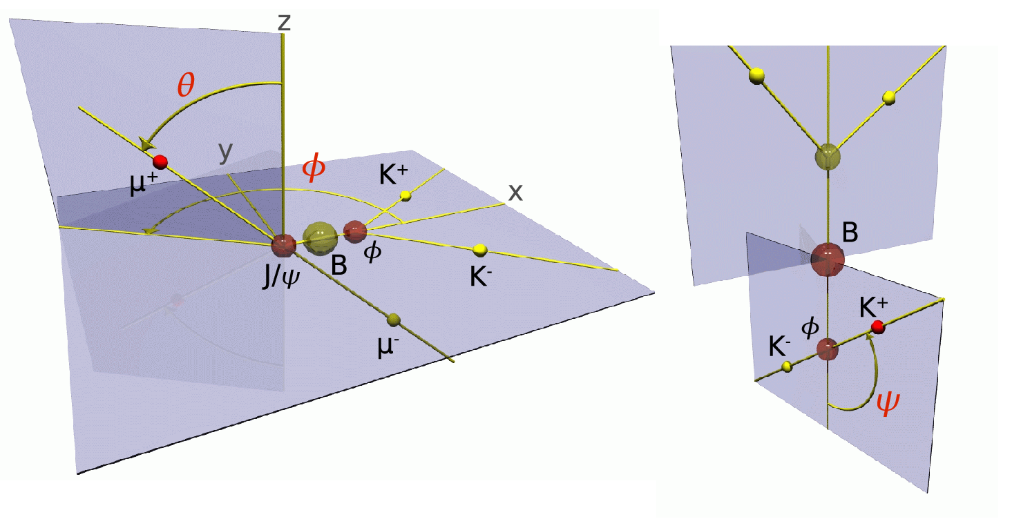
Since is a pseudo-scalar meson, and are both vector mesons, the final states form a admixture of eigenstates, where and waves are even, while wave is odd. To separate the two eigenstates, we analyze the angular distribution in the transversity basis. In this basis, the final state consists of three orthogonal polarization states, such that the two final state vector mesons are either longitudinally polarized, transversely polarized and perpendicular to each other, or transversely polarized and parallel to each other. Transitions from the initial state to these polarization states are described by amplitudes (, , ). Three transversity angles defined in different rest frames as shown in Fig. 3 are the polar and azimuthal angles of positive muon in the rest frame, and the helicity angle of positive kaon in the rest frame.
III.3 Flavor Identification
and quarks are produced together in general through QCD at Tevatron. Two types of tagging algorithms are used at CDF. The first algorithm tags the quark that produces the candidate in the sample, which is called same side tagging (SST). The other algorithm, known as opposite side tagging (OST), tags the other quark. On the near side, the is usually associated with a charged kaon due to the fragmentation process, so the charge of the kaon can be used to identify the flavor. This algorithm is also called same side kaon tagging (SSKT). On the away side, the charge of leptons coming from semileptonic decay of hadrons, or the charge of the jet is correlated to the flavor.
The flavor tagging algorithms have limited analyzing power for several reasons. On the near side, a charged kaon is not always available, and has a background from charged pions. On the away side, both the oscillation of neutral mesons and the sequential decay of quark lead to incorrect flavor identification. Each tagging algorithm returns two things: 1) A decision () that identifies the flavor of the candidate. The fraction of the events with decision is called the tagging efficiency . 2) A quality estimate of that decision, called dilution . The probability to obtain a correct tag is . The OST efficiency is around 96%, with an average dilution around 11%, while the SSKT efficiency is around 51%, with an average dilution around 27%. The total effective tagging power is characterized by .
IV MEASUREMENT WITH FLAVORING TAGGING
The decay of the meson depends on both time and angular distribution, and the decay probability density function for can be expressed as
| (11) | |||||
where , and functions are related to angular distribution. The probability density function for is obtained by substituting and . The time dependent term is defined as
where for and for . Other time independent terms are
where , , and is the mass difference of the two mass eigenstates which will be constrained to the CDF measurement result [9]. An unbinned maximum likelihood fit is performed to extract the parameters of interest: violation phase and decay width difference of the two mass eigenstates. The resolution effects and detector efficiencies are also incorporated into the likelihood function [10].
Without flavor tagging, a four-fold ambiguity will arise from the likelihood function, and the sensitivity to is marginal. At CDF, the measurement without flavor tagging is performed with integrated luminosity of 1.7 fb-1. The final result as shown in the Fig. 4 (left) is a two dimensional confidence region of and . The standard model prediction of [11] is consistent with the data at probability of 22% or 1.2 level. The details of the measurement can be found in Ref. [12].


The measurement can be improved with flavor tagging, where one will expect better sensitivity, since we obtain information on and separately. However, a two-fold ambiguity still remains with the simultaneous transformation (). This symmetry, combined with limited statistics, precludes a point estimate of the physics parameters and ; instead, a confidence region is obtained. The two dimensional confidence region of and is shown in the Fig. 4 (right), where the standard model prediction point has probability 15%, equivalent to 1.5 Gaussian standard deviation. If is treated as a nuisance parameter, we obtain a one dimensional confidence region of , where at 68% confidence level.
V CONCLUSION
The first violation phase measurement from flavor tagged decays has been presented. The result is consistent with the standard model, but only at 15% confidence level. Since the HCP conference, CDF has updated its result to 2.8 fb-1 of data which shows the result is consistent with the standard model only at 7% confidence level [13].
Acknowledgements.
I would like to thank the organizers of HCP 2008 conference for a enjoyable week. I also would like to thank all my colleagues at CDF collaborations and Fermilab staff for their hard work which makes these results possible.References
- [1] J. H. Christenson, J. W. Cronin, V. L. Fitch and R. Turlay, Phys. Rev. Lett. 13, 138 (1964).
- [2] N. Cabibbo, Phys. Rev. Lett. 10, 531 (1963).
- [3] M. Kobayashi and T. Maskawa, Prog. Theor. Phys. 49, 652 (1973).
- [4] L. Wolfenstein, Phys. Rev. Lett. 51, 1945 (1983).
- [5] B. Aubert et al., [BABAR Collab.], Phys. Rev. Lett. 87, 091801 (2001).
- [6] K. Abe et al., [Belle Collab.], Phys. Rev. Lett. 87, 091802 (2001).
- [7] C. Liu [CDF Collaboration and D0 Collaboration], arXiv:0806.4786 [hep-ex].
- [8] D. Acosta et al. (CDF Collaboration), Phys. Rev. D 71, 032001 (2005).
- [9] A. Abulencia et al. (CDF Collaboration) Phys. Rev. Lett. 97, 242003 (2006).
- [10] T. Aaltonen et al. [CDF Collaboration], Phys. Rev. Lett. 100, 161802 (2008) [arXiv:0712.2397 [hep-ex]].
- [11] A. Lenz and U. Nierste, J. High Energy Physics. 06, 072 (2007).
- [12] T. Aaltonen et al. [CDF collaboration], Phys. Rev. Lett. 100, 121803 (2008) [arXiv:0712.2348 [hep-ex]].
- [13] http://www-cdf.fnal.gov/physics/new/bottom/bottom.html