Light-like Wilson Loops and Cusp Anomalous Dimensions in Nonconformal Gauge Theories
Abstract
We emphasize that nonconformal theories provide a natural playground for the ideas of the Maldacena conjecture opening the possibility of exploring properties that could potentially be in the same universality class as QCD. In particular, we discuss in detail how light-like Wilson loops, an important ingredient in the prescription for scattering amplitudes, can be described in a number of gravity duals of nonconformal gauge theories. We point out to a few universal properties and the prominent role of the strong scale.
Keywords:
Gauge/string duality, Strong-coupling expansions, Wilson loopsClassification:
11.25.-w,11.25.Tq,11.15.Me1 Introduction
The idea that the description of gauge theories might effectively involve strings has a long history starting from the dual models for hadronic resonances. In 1974 ‘t Hooft [1] showed that gauge theories admit a limit in which their perturbation theory can be thought of as coming from a string theory. Ten years ago, a precise formulation of this equivalence was put forward for a particular gauge theory. Namely, it was argued that supersymmetric Yang-Mills (SYM) is dual to type IIB string theory propagating on [23, 32, 10]. In the ten years following the seminal work of Maldacena [23] the gauge/gravity correspondence has seen a period of maturity. In its current incarnation the correspondence has turned into a very fruitful theoretical framework.
Particularly exciting is the side of Maldacena’s conjecture relating the strongly coupled sector of the gauge theory with weakly coupled gravity. Many problems in gravity have been solved during nearly a century of work. By turning strong coupling problems of gauge theories into questions in classical gravity, the correspondence opened a window of opportunity into one of the long-standing puzzles of particle physics: the infrared properties of gauge theories. Some of the questions to be addressed here are confinement, the spectrum of hadrons and the properties of the strongly coupled quark-gluon plasma. However, important questions about nonprotected quantities lie beyond the domain of classical gravity and should properly be tackled using string theory.
There are two main obstacles in applying the gauge/gravity correspondence to phenomenologically interesting theories. The high amount of supersymmetry and conformal symmetry is not present in nature. Although originally formulated as a duality between string theory on and maximally SYM in four dimensions, it has quickly become clear that such dualities extend to more general situations. Significant results in understanding QCD-like theories have been achieved by constructing supergravity theories whose dual gauge theories contain , supersymmetric Yang-Mills [25, 13]. In a remarkable series of papers [19] Klebanov and collaborators carried out a program that concluded with a supergravity background that is dual to supersymmetric gauge theory that displays confinement and chiral symmetry breaking in the IR. This background is known as the warped deformed conifold or the Klebanov-Strassler (KS) solution. In the UV this background encodes a series of Seiberg duality cascades in the field theory. A fairly comprehensive description of how to encode gauge dynamics into supergravity backgrounds was presented by Sonnenschein and Loewy in [20]. They analyzed the following properties: gauge group, supersymmetries, Wilson and ‘t Hooft loops and the corresponding quark anti-quark or monopole anti-monopole potentials, instantons and the symmetry breaking, gluino condensation and spontaneous breaking, monopoles, domain walls, baryons and KK states. Moreover, a supergravity solution dual to the finite temperature warped conifold with cascading in the UV was found [27]. Evidence of a transition between this solution and the KS solution was reported in [21] (see also [2]). Such transition could be interpreted as the gravity dual to the confinement/deconfinement transition in QCD-like theories.
Another important direction in which the Maldacena conjecture has been expanded is in going beyond the lowest energy states. Much of the developments in the conformal version regarding beyond the supergravity approximation were extended to the nonconformal case. For example, the BMN limit [5] was also understood in nonconformal situations; the analogous structure describes hadronic states for which an exact string Hamiltonian was presented [8]. Using semiclassical quantization in the context of gauge/gravity correspondence, quantum corrections to Regge trajectories were calculated [26], showing that quantum effects alter both the linearity of the trajectory and the vanishing classical intercept, .
More recently, Alday and Maldacena proposed a prescription to calculate the gluon scattering amplitudes for using beyond the supergravity degrees of freedom [3]. Further research in that direction has already gained momentum (for instances and references see the contribution by Alday and Maldacena to this volume). The logical next step is to apply their prescription to nonconformal situations. However, several obstacles arise. First of all, we have to deal with less symmetry, meaning that we need to use more powerful techniques to solve the corresponding problems. Fortunately, these problems reduce to systems of ordinary and partial differential equations, and we can use many analytical and numerical methods for studying and solving them.
One goal of this contribution is to display the power of these methods. Using as illustrative examples the Witten-QCD [33] and KS [13] models, we are going to show that analysis of the light-like Wilson loop in the dual momentum space for nonconformal situations shows some universal properties. Based on the recognizable universality that we obtain, we expect that the analysis of gluon scattering in nonconformal theories would also yield valuable results potentially in the same universality class as QCD.
2 Wilson loops in gauge theories
The Wilson loop is a very important observable in gauge theories and in some approaches it is treated as the central ingredient in the description of all gauge invariant quantities. Its description on the gravity side was proposed in [24, 29] where it was suggested that the evaluation of the vacuum expectation value of a given Wilson loop on the contour is given by the string worldsheet whose boundary coincides with : .

The Wilson loop provided the first example of the correspondence that goes beyond the study of protected quantities at the supergravity level. Related developments allowed to understand that certain non-BPS operators can be described by classical string configurations in a given supergravity background. For example, the large anomalous dimension of operators of the form , where are scalar fields in SYM, was computed in [11] by considering a large closed string spinning in ,
| (1) |
where is the ’t Hooft coupling. These operators are generalizations in SYM of the twist-two operators that play a central role in the deep inelastic scattering in QCD [7, 9]. They appear in the operator-product expansion of two electromagnetic currents and . Soon after [11], a description of these operators was found in terms of light-like Wilson loops in the AdS/CFT correspondence [16, 22]. One important property of the anomalous dimensions of these operators is that it is conjectured to be in general of the form , where is the cusp anomalous dimension and it is a function only of .
The Alday-Maldacena prescription for gluon scattering in SYM [3] involves computations of classical worldsheets in that end on light-like segments. These configurations are light-like Wilson loops. It is crucial that the space where these Wilson loops live is the T-dual space to the original supergravity background. This construction motivates us to revisit and expand the analysis of worldsheet configurations ending on light-like segments in supergravity backgrounds dual to nonconformal theories. Similar configurations have been considered before but with two main differences from those we present here. First, they were considered in the original supergravity background, that is, without performing a T-duality and second the light-like segments were always placed in the asymptotic UV region. For example, the light-like Wilson loop on the Klebanov-Strassler background was analyzed in [17].
In this contribution we report on the situation where we perform a T-duality on the subspace where the field theory lives, and the light-like segments are placed in the region corresponding to the IR of the field theory. Since we work on the T-dual space and place the brane in an arbitrary position, the value of the cusp depends on the structure of the infrared region. This is a crucial difference with perturbative QCD where no access to the IR region is possible other than on dimensional grounds.
2.1 Cusps anomalous dimension
If a Wilson loop is evaluated over a closed contour that forms a light-like cusp with angle in Minkowski space-time, then its expectation value is [28],
| (2) |
where is a UV cutoff, is an IR cutoff, and measures the anomalous dimension of the Wilson loop. The cusp anomalous dimension is also an important observable in gauge theories. It controls the scaling behavior of various gauge invariant quantities like the logarithmic scaling of the anomalous dimension of higher-spin Wilson operators, double-log (Sudakov) asymptotics of elastic form factors in QCD, the gluon Regge trajectory, infrared asymptotics of on-shell scattering amplitudes, and it is important for resumming the effects of soft gluon emission in the study of QCD at colliders [15].
The cusp anomalous dimension depends only on the coupling constant and its expansion at weak coupling is known in QCD to three loops [31] and in SYM to four loops [6]. In the strong coupling regime of SYM it was calculated to lowest order in [11, 16, 22], and to higher orders in [18, 30]. In the strong coupling regime of cascading theories the first results were obtained in [17]. For our results we needed to generalize this last approach by putting the brane in a different position. In the future we plan to calculate the scattering amplitudes and at that point we actually will require a surface instead of an infinitely extending cusp, that is, the surface for scattering ends on cusps and thus the surface does not extend to infinity.
In this note we report mostly on work performed for WQCD and the KS backgrounds. However, for the strategy of understanding which precise properties of nonconformal theories are universal and which are model-dependent, it is important to discuss various cases. We are currently analyzing also the cases of the nonconfining cascading solution of [27], the noncritical background [4] and the noncritical solution with an infrared fixed point [14].
2.1.1 The general set up for the cusp
Let us consider a general metric of the form: . We perform a T-duality along the coordinates and arrive at a metric of the form
| (3) |
We now consider embedding a string world sheet into this metric. For world sheet coordinates , this embedding is , , . The action is thus
| (4) |
The methodology is then to derive the equation of motion for , to solve it, substitute the solution into (4) and integrate for the action. This integral typically diverges, so an UV cutoff must be chosen as upper limit of integration. Given that , the cusp anomalous dimension can be obtained from (2) as,
| (5) |
2.1.2 The cusp in SYM
Here we present elements of a systematic analysis to the derivation of the solution for this most symmetric case. It might seem like an overkill, however, reproducing analytical results for simple cases helps to adjust the numerical methods for handling less symmetric situations. Here we study a building block for the configuration that leads to the scattering amplitude.
Let us consider the cusp as described in [3]. For we have that in (4) and . Moreover, if we consider an ansatz of the type , then we find that the action is:
| (6) |
Following the methodology listed at the end of the previous subsection we derive the corresponding equation of motion which, for the purpose of numerical integration, is better to write as the following system of first order ordinary differential equations,
| (7) |
Here dot stands for derivative with respect to . We solved this system using the seventh-eight order continuous Runge-Kutta method. Thanks to its adaptive scheme, this method provides a great control upon the output accuracy. Typical solutions are plotted in fig.2.


An important point here is that numerical solutions are not necessarily black boxes. Qualitative and asymptotic analysis help to understand the numbers which in turn might guide the analysis. For instance, in this case we can use the theory of dynamical systems to understand the contents of figures 2. This theory includes a set of general techniques for the analysis of phase spaces that allows us to understand better the asymptotics of solutions and their dependence on the initial conditions. This is a natural way of tackling problems about classical solutions in string theory; we are not aware of previous works emphasizing these systematic methods; most of the literature emphasizes exploiting symmetries. While of paramount importance in , most symmetries are lacking in the context of supergravity backgrounds dual to nonconformal theories.
Setting the vector field to zero in system (7), we see that there are two fixed points. They are respectively located at and . If these singular points were hyperbolic, then the Hartman-Grobman theorem [12] ensures that, in a small neighborhood of each hyperbolic fixed point, the flow defined by the full nonlinear system (7) is topologically equivalent to its linearized version. A singular point is hyperbolic if the eigenvalues of the Jacobian of the linearization around the point have non-zero real parts. For the first point we obtained and . This indicates that in its neighbourhood the flow behaves like near a radial sink (stable node), as it is shown in the center of fig.2. For the second singular point and . So, in its neighborhood the flow behaves like near a saddle point, as shown to the right in fig.2.
Having tested that the numerical and analytical results coincide, we can move forward and integrate (6) numerically. Taking , we evaluate the action with a set of different upper limits which are defined by . Then using , we estimate the cusp anomalous dimension using (5). The outcome for this case nicely replicates the result in [3]. Because of lack of space, we refrain of presenting it here, and move forward to the nonconformal cases.
3 Cusp anomalous dimensions in nonconformal gauge theories
3.1 Witten QCD
In this subsection we calculate the cusp anomalous dimension for the Witten background [33]. With that aim we rewrite the metric in the relevant IR regime. The ten-dimensional string frame metric and dilaton of this model are
| (8) |
The geometry consists of a warped, flat 4-d part, a radial direction , a circle parameterized by with radius vanishing at the horizon , and a four-sphere whose volume is instead everywhere non-zero. It is non-singular at . In the limit the dilaton diverges: this implies that in this limit the completion of the present IIA model has to be found in M-theory. The background is completed by a constant four-form field strength , where is the volume form of the transverse .
The main gauge theory parameter we will use in the following is the KK mass scale , where . As can be read from the metric, is also the typical glueball mass scale, and its square is proportional to the ratio between the confining string tension and the UV ’t Hooft coupling . The supergravity approximation works in the regime opposite to that in which the KK degrees of freedom decouple from the low energy dynamics. Condition implies , which is beyond the supergravity regime of validity.
Assuming that , with , , and introducing the new coordinate , so that , the action (4) is now:
| (9) |
A convenient way to write the equation of motion is:
| (10) |
where and are now measured in units of , and a dot stands for derivative with respect to . Note that is not properly a fixed point of the action. A typical solution of this second order non-linear non-autonomous equation is presented in the left of fig.3.


As with the rest of the examples plotted in this subsection, it was obtained by setting , , and . To understand this result let us analyze the asymptotic regimes.
3.1.1 Asymptotic behavior of the solution
First, we look for a solution for and . Balancing equation (10) the relevant terms are,
| (11) |
For this balance to be consistent it is required the absolute value of the second derivative to be greater than the neglected terms. It can be readily tested that this condition is fulfilled in the limits of and we are considering.
We inmediately note that any solution to (11) with initial condition at is a constant solution. A solution to this equation given as an expansion in Taylor series is,
| (12) |
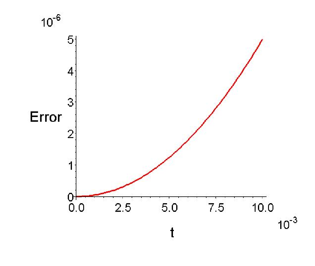
It can be seen that, in the limit , actually acts as a fixed point of the system. We tested this result numerically. In the center of fig.3 we can see that the difference between (12) and a corresponding numerical solution is negligible. Thus, the approximation works in the range of and considered.
Let us now consider the asymptotic behavior of the solution for Now the equation of motion (10) becomes
| (13) |
With regards to the consistency of this balance, from fig.3 it can be assumed that the large behavior of the solutions is linear. Then, the second derivative goes to zero and that is also true for the neglected terms, For further verification we again compare the analytical and numerical results. Note now that the second derivative is zero when the first derivative is whose limit as gives . So, for any , some solutions converge to a linear solution with slope and some diverge from a linear solution with slope . In the right of fig.3 the phase-space of (13) is plotted. We see that, indeed, for any , is an attractive set and that the solutions diverge from . Now, recall that we are analyzing the behavior for and, according to the analysis of the solutions when , the interesting us region is and . It means that the interesting us asymptotic behavior is given by the linear solution with slope equal to .
Summarizing, the analysis and the numerical results for the range of tested ( and ) indicate that the generic behavior of the solutions is as follows: acts as a fixed point of this system; with an initial condition near , the solution starts with a regime where . Next there is a transient regime where the solution smoothly changes until it finally sets into a linear behavior with unit slope. The closer the initial condition to the horizon, the larger the length of the initial regime and the shorter the transition regime. The length of the time intervals are to be considered relatively, since the figures show always the same behavior if the right lengths of the interval are chosen.
3.1.2 The cusp anomalous dimension
Next, following our methodology, we evaluate the numerical solution in the action and integrate it numerically. To accurately compute the actions we used an adaptive 3-5 Simpson’s quadrature. If numerical factors are not taken into account, the integrand is, We have already seen that while . Therefore, if we expect this integral to diverge logarithmically, we need the argument of the squared root to behave like . Indeed, using a best fit to the numerical results, we have verified that this is the case, and we present an example in the left side of fig.4. In the center


a typical result for the action as a function of is plotted.
The coefficient of is , where stands for the numerical factors in front of the integral, , and . The numbers were obtained by the best fit shown in the right of fig.4.
3.2 The warped deformed conifold
The Klebanov-Strassler background [13] is very well known in the literature of gravity duals to confining gauge theories, a full presentation of its metrics and action, suited for numerical calculations can be found in the appendix A of [21].
Using coordinates where and setting , the equation of motion for this background is
| (14) | |||
This equation was solved by setting and , and then using a fourth order Runge-Kutta method for the evolution of the solution as a function of . The numerical integration necessary for evaluating the warp factor was done using a composite Simpson method. A typical solution is presented in fig.5.

An analysis similar to the previous subsections shows that there is a fixed point at . The solution initially stays close to the fixed point, then there is a transition to a logarithmic looking function. The region close to the fixed point is larger depending on how close to the fixed point the solution begins.
To show that the solution grows logarithmically, we examine the form of the metric for large . In this regime, is also getting large, so we have , where is a constant. The KS metric now has the form Substituting and performing a T-duality on the coordinates, the metric is
| (15) |
Now, in the large (large ) approximation where is a constant, and one gets
| (16) |
which is with a logarithmic prefactor. To a first approximation, we can ignore the prefactor which will change slowly, to the metric, to see that the cusp solution of which is will hold, which means that for large .
This way, the result for KS resembles very much the one obtained for WQCD.
4 Discussion and outlook
In this contribution we have shown that light-like Wilson loops in nonconformal theories display some rather universal features. We hope that this is the kind of question that can be asked and whose answer should be trusted to be in the same universality class as QCD. The light-like Wilson loops we have considered here are building blocks of the scattering amplitudes. We hope, as is the case in the perturbative treatment of QCD amplitudes, that the main contribution to scattering amplitudes will come from the cusp region and therefore, our calculations will be a crucial building block in the amplitudes.
It is important to note that, although not included in this contribution, we have performed similar analysis for various theories and the behavior is rather similar to the one observed in the two examples considered explicitly here. Basically, there is a natural infrared regulator which is characterized by the distance between the position of the brane and the characteristic strong scale which in most supergravity solutions is given by the region where a cycle collapses ( for WQCD and for KS). We want to emphasize that in the perturbative approach to gauge theories the infrared regulator normally used is formal and has nothing to do directly with the strong scale. We thus hope that our strong coupling calculation will help shed some light into the structure of IR singularities.
References
- [1] Cited by: §1.
- [2] Cited by: §1.
- [3] Cited by: §1, §2.1.2, §2.1.2, §2.
- [4] Cited by: §2.1.
- [5] Cited by: §1.
- [6] Cited by: §2.1.
- [7] Cited by: §2.
- [8] Cited by: §1.
- [9] Cited by: §2.
- [10] Cited by: §1.
- [11] Cited by: §2.1, §2, §2.
- [12] Cited by: §2.1.2.
- [13] Cited by: §1, §1, §3.2.
- [14] Cited by: §2.1.
- [15] Cited by: §2.1.
- [16] Cited by: §2.1, §2.
- [17] Cited by: §2.1, §2.
- [18] Cited by: §2.1.
- [19] Cited by: §1.
- [20] Cited by: §1.
- [21] Cited by: §1, §3.2.
- [22] Cited by: §2.1, §2.
- [23] Cited by: §1.
- [24] Cited by: §2.
- [25] Cited by: §1.
- [26] Cited by: §1.
- [27] Cited by: §1, §2.1.
- [28] Cited by: §2.1.
- [29] Cited by: §2.
- [30] Cited by: §2.1.
- [31] Cited by: §2.1.
- [32] Cited by: §1.
- [33] Cited by: §1, §3.1.
References
- (1) G. ’t Hooft, Nucl. Phys. B 72, 461 (1974).
- (2) J. M. Maldacena, Adv. Theor. Math. Phys. 2 (1998) 231 [Int. J. Theor. Phys. 38 (1999) 1113] [arXiv:hep-th/9711200].
- (3) E. Witten, Adv. Theor. Math. Phys. 2, 253 (1998) [arXiv:hep-th/9802150].
- (4) S. S. Gubser, I. R. Klebanov and A. M. Polyakov, Phys. Lett. B 428 (1998) 105 [arXiv:hep-th/9802109].
- (5) J. M. Maldacena and C. Nunez, Phys. Rev. Lett. 86, 588 (2001) [arXiv:hep-th/0008001].
- (6) I. R. Klebanov and M. J. Strassler, JHEP 0008 (2000) 052 [arXiv:hep-th/0007191].
- (7)
I. R. Klebanov and E. Witten,
Nucl. Phys. B 536 (1998) 199
[arXiv:hep-th/9807080].
S. S. Gubser and I. R. Klebanov, Phys. Rev. D 58 (1998) 125025 [arXiv:hep-th/9808075].
I. R. Klebanov and N. A. Nekrasov, Nucl. Phys. B 574 (2000) 263 [arXiv:hep-th/9911096].
I. R. Klebanov and A. A. Tseytlin, “Gravity duals of supersymmetric SU(N) x SU(N+M) gauge theories,” Nucl. Phys. B 578 (2000) 123 [arXiv:hep-th/0002159]. - (8) A. Loewy and J. Sonnenschein, JHEP 0108, 007 (2001) [arXiv:hep-th/0103163].
- (9) L. A. Pando Zayas and C. A. Terrero-Escalante, JHEP 0609, 051 (2006) [arXiv:hep-th/0605170].
- (10) M. Mahato, L. A. Pando Zayas and C. A. Terrero-Escalante, JHEP 0709, 083 (2007) [arXiv:0707.2737 [hep-th]].
- (11) O. Aharony, A. Buchel and P. Kerner, Phys. Rev. D 76, 086005 (2007) [arXiv:0706.1768 [hep-th]].
- (12) D. E. Berenstein, J. M. Maldacena and H. S. Nastase, JHEP 0204, 013 (2002) [arXiv:hep-th/0202021].
- (13) E. G. Gimon, L. A. Pando Zayas, J. Sonnenschein and M. J. Strassler, JHEP 0305, 039 (2003) [arXiv:hep-th/0212061].
- (14) L. A. Pando Zayas, J. Sonnenschein and D. Vaman, Nucl. Phys. B 682, 3 (2004) [arXiv:hep-th/0311190].
- (15) L. F. Alday and J. M. Maldacena, JHEP 0706 (2007) 064 [arXiv:0705.0303 [hep-th]].
- (16) E. Witten, Adv. Theor. Math. Phys. 2 (1998) 505 [arXiv:hep-th/9803131].
- (17) J. M. Maldacena, Phys. Rev. Lett. 80 (1998) 4859 [arXiv:hep-th/9803002].
- (18) S. J. Rey and J. T. Yee, Eur. Phys. J. C 22 (2001) 379 [arXiv:hep-th/9803001].
- (19) S. S. Gubser, I. R. Klebanov and A. M. Polyakov, Nucl. Phys. B 636 (2002) 99 [arXiv:hep-th/0204051].
- (20) H. Georgi and H. D. Politzer, Phys. Rev. D 9 (1974) 416.
- (21) D. J. Gross and F. Wilczek, Phys. Rev. D 9, 980 (1974).
- (22) M. Kruczenski, JHEP 0212 (2002) 024 [arXiv:hep-th/0210115].
- (23) Y. Makeenko, JHEP 0301 (2003) 007 [arXiv:hep-th/0210256].
- (24) M. Kruczenski, Phys. Rev. D 69 (2004) 106002 [arXiv:hep-th/0310030].
- (25)
A. M. Polyakov,
Nucl. Phys. B 164 (1980) 171.
S. V. Ivanov, G. P. Korchemsky and A. V. Radyushkin, Yad. Fiz. 44, 230 (1986) [Sov. J. Nucl. Phys. 44, 145 (1986)]. - (26) G. P. Korchemsky and G. Marchesini, Nucl. Phys. B 406 (1993) 225 [arXiv:hep-ph/9210281].
- (27) A. Vogt, S. Moch and J. A. M. Vermaseren, Nucl. Phys. B 691 (2004) 129 [arXiv:hep-ph/0404111].
- (28) Z. Bern, L. J. Dixon, D. A. Kosower, R. Roiban, M. Spradlin, C. Vergu and A. Volovich, arXiv:0803.1465 [hep-th].
- (29) M. Kruczenski, R. Roiban, A. Tirziu and A. A. Tseytlin, Nucl. Phys. B 791 (2008) 93 [arXiv:0707.4254 [hep-th]].
- (30) R. Roiban and A. A. Tseytlin, JHEP 0711 (2007) 016 [arXiv:0709.0681 [hep-th]].
- (31) S. K. Ashok, S. Murthy and J. Troost, Nucl. Phys. B 749 (2006) 172 [arXiv:hep-th/0504079].
- (32) I. R. Klebanov and J. M. Maldacena, Int. J. Mod. Phys. A 19 (2004) 5003 [arXiv:hep-th/0409133].
- (33) J. Guckenheimer and P. Holmes, ”Nonlinear Oscillations, dynamical systems and bifurcations,” Springer-Verlag, 1983, 235pp.