Canonical Relativity
and the Dimensionality of the World**
*
In: Relativity and the Dimensionality of the
World, Ed. V. Petkov (Springer, 2007), pp. 137–152
Martin Bojowald
Institute for Gravitation and the Cosmos,
The Pennsylvania State University,
104 Davey Lab, University Park, PA 16802, USA
Abstract
Different aspects of relativity, mainly in a canonical formulation, relevant for the question “Is spacetime nothing more than a mathematical space (which describes the evolution in time of the ordinary three-dimensional world) or is it a mathematical model of a real four-dimensional world with time entirely given as the fourth dimension?” are presented. The availability as well as clarity of the arguments depend on which framework is being used, for which currently special relativity, general relativity and some schemes of quantum gravity are available. Canonical gravity provides means to analyze the field equations as well as observable quantities, the latter even in coordinate independent form. This allows a unique perspective on the question of dimensionality since the space-time manifold does not play a prominent role. After re-introducing a Minkowski background into the formalism, one can see how distinguished coordinates of special relativity arise, where also the nature of time is different from that in the general perspective. Just as it is of advantage to extend special to general relativity, general relativity itself has to be extended to some theory of quantum gravity. This suggests that a final answer has to await a thorough formulation and understanding of a fundamental theory of space-time. Nevertheless, we argue that current insights into quantum gravity do not change the picture of the role of time obtained from general relativity.
1 Introduction
When faced by the question of whether the world is three- or four-dimensional, the quick answer by a modern-day physicist will most likely be ‘‘four.’’ This is indeed what relativity tells us formally where space and time are essentially interchangeable: Lorentz transformations, or their physical manifestations of Lorentz contraction and time dilatation, show that space and time not only play similar roles but can even be transformed into each other. Just as we can rotate a body in three dimensions to observe all its extensions, thereby transforming, e.g., its height in width, we can boost an object11 1 By “object” we will mean a physical system defined by a set of observable properties such that it can be recognized at different occurrences in space and in time. Objects will not be idealized to be point-like or event-like in order to remain unbiased toward the question of dimensionality. Thus, non-vanishing extensions of objects in space as well as time are allowed in order to take into account the necessary unsharpness of measurements needed to verify the defining properties. so as to, at least to a certain extent, replace space-like by time-like extension and vice versa. The qualification “to a certain extent” is necessary because even in relativity space and time are not quite the same but distinguished by the signature of the space-time metric. By itself, this difference in signature is not sufficient reason to deny time the same ontological status as space.
There are, however, differences between the usual treatment of space and time in physics going beyond relativity, although they are usually presupposed in relativistic discussions. In order to answer the question of the dimensionality of the world from the viewpoint of relativity, such hidden assumptions have to be uncovered and analyzed, or avoided altogether. Some of these issues lie at the forefront of current physics and still await explanation. For instance, while we can, and have to, limit objects to finite spatial extensions, we have no means to limit their time extensions safe for transformations such as particle decay or other reactions. Even though objects may change in time, they never cease to exist completely. There seems to be a simple reason for that: conservation laws. We simply cannot limit an object’s extension in time because, e.g., its energy must be conserved. Thus, the object could be transformed into something else of the same energy but not removed completely. Such laws are derived as consequences of symmetries which first give local conservation laws in terms of currents. Going from local to global conservation laws, as they are required for an explanation of the persistence of objects in time, is a further step and requires additional assumptions. As the following more detailed discussion shows, conservation laws cannot be used to explain the difference of spatial and time-like extensions, for the derivation itself distinguishes space from time.
One starts with a local equation such as22 2 We follow the abstract index notation common in general relativity (see, e.g., [1]). Indices refer to space-time while indices used later refer only to space. Repeated indices occurring once raised and once lowered are summed over the corresponding range for space-time indices and for space indices. The covariant derivative compatible with a given space-time metric is denoted by which for Minkowski space reduces to the partial derivatives in Cartesian coordinates. for the energy-momentum tensor . If the space-time metric is sufficiently symmetric and allows a Killing vector field satisfying , the current is conserved: . At this stage, the only difference between space and time enters through the signature of the metric. A global conservation law is then derived by integrating the local conservation equation over a space-time region bounded by two spatial surfaces and and some boundary which could be at infinity. Stokes theorem then shows that the quantity is the same on and and thus conserved, provided that all fields fall off sufficiently rapidly toward the boundary . Thus, one already has to assume physical objects to be of finite spatial extent before obtaining a global conservation law, while there is no such restriction for the time-like extension.33 3 In this discussion we understood, as usually, that space-time is Minkowski as in special relativity. The energy conservation argument in our context works better if one considers instead a universe model with compact spatial slices, such as an isotropic model with positive spatial curvature, or a compactification of isotropic models of non-positive curvature. This requires one to go beyond special relativity, as we will do later on for other reasons, and to allow non-zero curvature or non-trivial topology. From our perspective, closed universe models are conceptually preferred because space is already finite without boundary such that non-spacelike boundaries are not needed to derive global conservation laws from local ones. If fields do not vanish at , one interprets as the flux into or out of the spatial region evolving from to . However, this different interpretation of as conserved quantity on and and as flux on treats space and time differently, corresponding to the non-relativistic decomposition of energy-momentum in energy and momentum. This different treatment is not implied by the theory but put in by interpreting its objects. The issue of a limited spatial extent versus unconstrainable duration of objects thus remains and has to be faced even before coming to conservation laws.

For this reason, it seems to be potentially misleading to consider objects in space-time such as point particles or their worldlines to address the dimensionality of the world, for there are already presuppositions about space and time involved. Indeed, from this perspective a worldline, or the world-region of an extended object, seems inadequate for a relativistic treatment. It would be more appropriate to use only either space-time events or bounded four-dimensional world-regions of extended objects. This already indicates a possible answer to the question of dimensionality: events are zero-dimensional and to be considered as idealizations just as their analogs of point particles. The only option then is to consider bounded world-regions44 4 Indeed, to analyze an object by whatever means we not only need to capture it at one time — which is virtually impossible, anyway — but also hold and observe it for some time. Observations thus always refer to some finite extension in time during which we must be able to recognize the system. A good example can be found in particle physics where too short decay times imply that particles appear rather as resonances without sharp values for all their properties. This is a consequence of uncertainty and thus quantum theory which we will come back to later. Even though common terminology often assigns the object status to an isolated system at a given time, evolving and possibly changing, observations always consider world-regions which could be assigned the object status as well. This non-traditional use of the term “object” is probably discouraged because it is too observer-dependent: it is the observer who decides when to end the experiment and thus determines the time-like extension of the space-time region. However, while the classical world allows us to draw sharp spatial boundaries and thus seems to imply individualized spatial objects, this is no longer possible in a quantum theory. Drawing the line around spatial objects is then a matter of choice, too, comparable to limiting the duration of an observation. as physical objects, which are four-dimensional.
It is difficult to follow these lines toward a clear-cut argument for the four-dimensionality of the world due to our limited understanding of the nature of time. An alternative approach is to disregard objects in space-time and rather consider the relativistic physics of space-time itself. For this, we need general relativity which, compared to special relativity, has the added advantage of removing the background structure given by assuming Minkowski space-time. As backgrounds can be misleading, if possible one should consider the more general situation and then see how special situations can be re-obtained.
The following sections collect possible ingredients which can be helpful in the context of dimensionality. There are different formulations of general relativity, covariant and canonical ones, which apparently reflect the possible interpretations of a four-dimensional versus a three-dimensional world: While covariant field equations are given on a space-time manifold, the canonical formulation starts with a slicing of space-time in a family of spatial slices. Canonical fields are then defined on space and evolve in time, suggesting a three-dimensional world with an external time parameter [2]. Nonetheless, the question of dimensionality cannot be answered easily because, for one thing, the formulations are mathematically equivalent. In what follows, we will mainly use canonical relativity so as to see if it indeed points to a three-dimensional world or, as the covariant formulation, a four-dimensional one. Covariant formulations are also best suited to understand the relativistic kinematics and dynamics. After this general exposition we will specialize the formalism to Minkowski space in order to see which freedom is eliminated in special relativity compared to general relativity and how this can change the picture of time. We end with a brief discussion of dynamical consequences of general relativity as well as some comments on quantum aspects.
2 Canonical Relativity
The signature of the metric also has implications for the form of relativistic field equations on a given space-time which are hyperbolic rather than elliptic. This means that a reasonable set-up for solving these equations is by an initial value problem: for given initial values on space at an initial time one obtains a unique solution. For our purposes, this aspect is not decisive because we could interpret initial values as corresponding to objects placed in space before starting an observation, thus corresponding to a three-dimensional world, or simply as labels to distinguish solutions which themselves play the role of objects of a four-dimensional world.55 5 In fact, this is clearly brought forward by the canonical formulation where one can either specify states by a phase space given by initial data on the initial surface, or by the so-called covariant phase space consisting of entire solutions to the field equations. In both cases, the phase space is endowed with a symplectic structure, and the formulations are equivalent. The choice is then just a matter of convenience.
2.1 ADM Formulation
For the field equations of the metric itself the situation is more complicated and crucially different (see [3] for the general relativistic initial value problem). Einstein’s equations correspond to ten field equations for the ten components of the space-time metric , a symmetric tensor. However, there are only six evolution equations containing time derivatives only of some components while the remaining equations are elliptic and do not contain time derivatives. Although there is no fixed coordinate system, it is meaningful to distinguish between time and space derivatives because, due to the signature of the metric, they are related to vector fields of negative and positive norm squared, respectively. Time evolution is described by an arbitrary timelike vector field while spatial slices of space-time are introduced as level surfaces of a time function such that . The space-time metric induces a spatial metric on each slice as well as covariant spatial derivatives. The spatial metric is most easily expressed as
| (1) |
where is the unit future-pointing timelike co-normal to a slice. These are only six independent components because is degenerate from the space-time point of view: . These are also precisely the components of the space-time metric whose time derivatives66 6 Time derivatives are understood as Lie derivatives with respect to the time evolution vector field . appear in Einstein’s equations.
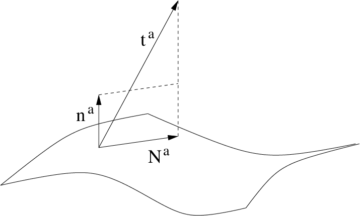
At this point, we may view the equations as describing the evolution of a three-dimensional quantity in an external time parameter . The remaining four space-time metric components encode the freedom in choosing the time evolution vector field, which can be parameterized as with components usually called lapse function and shift vector such that . They are indeed metric components since (1) implies
| (2) | |||||
The time-time component of the inverse space-time metric is thus while time-space components are . These components enter the field equations, too, but they are not dynamical in the sense that they would have evolution equations determining their time derivatives. In addition to the six evolution equations for ,
| (3) |
for the momenta conjugate to , there are then four constraint equations
| (4) |
which are of elliptic nature and restrict the values of the dynamical fields at any spatial slice (independently of and ).
A possible interpretation is that there are six fields on space which change in time as governed by the evolution equations, depending on four prescribed but arbitrary auxiliary fields and . This would be a mixed viewpoint as far as dimensionality is concerned because would look like spatial objects while and would have to be prescribed as functions of space and time but are not evolving in time. The system is thus rather four-dimensional since and have to be functions on a four-dimensional space and determine the evolution of for which only initial values on space are needed. One can save the three-dimensional interpretation by considering and as external functions for the evolution system of , but this has the drawback that there would be no predictivity and no uniqueness of solutions in terms of initial values for the dynamical fields, as solutions also depend on choices of and .
Here, the completely four-dimensional view is much more attractive: We not only have to choose the functions and but can also supplement the dynamical equations for by evolution equations for space-time coordinates. This is indeed possible, for if we choose four functions and and ask that they play the role of space-time metric components as they enter the canonical equations (2) we have the transformation laws
| (5) | |||||
| (6) |
from an arbitrary (inverse) space-time metric to the new functions. These transformations can be interpreted as evolution equations for the space-time coordinates which are then fixed by the choice of and in terms of coordinates on an initial spatial surface.77 7 Solutions depend on the auxiliary metric as well, as they should since no change in coordinates is necessary if had already been of canonical form with the chosen and . With this interpretation, we obtain, for given initial values, unique solutions to our evolution equations up to changes of coordinates, corresponding to a change in the free functions and .
The functions and which must be defined on a four-dimensional manifold thus determine coordinates such that canonical field equations for result. In general, there is no way to split this globally into a time coordinate and space-coordinates which one would need for a three-dimensional evolution picture of . Thus, a four-dimensional interpretation results. This attractive viewpoint is available only if we take as physical object on which field equations are imposed the entire space-time and not just the metric on spatial slices. We clearly have to consider general relativity which gives field equations for the metric and allows us to perform arbitrary coordinate changes, not just Lorentz transformations. Here, getting rid of the Minkowski background of special relativity, corresponding to a synchronization of rigid clocks and rulers throughout space-time under the assumption of the absence of a gravitational field, is required.
2.2 Relational Observables
Since we obtain a unique solution to the Einstein equations only up to arbitrary changes of space-time coordinates, predictivity requires observable quantities to be coordinate independent, too. While coordinates are usually used in explicit calculations, values of observable quantities must not change when transforming to different coordinates. Abstractly, one can also formulate the concept of an observable in an explicitly coordinate-free manner leading to relational observables: evolution is then measured not with respect to coordinate time but with respect to other geometrical or matter quantities. While this is appealing conceptually, it can be hard to do explicitly.88 8 “Such a question can, we are assured, always be answered from a sufficient set of initial data, though the performance of this task may call for considerable mathematical agility.” [4]. For instance, in a cosmological situation one can measure how the value of a matter field changes with respect to a change in the total spatial scale or volume. Since in such a picture coordinates are eliminated, an alternative view on the question of dimensionality is possible. It also allows us to show, as we will see, how Minkowski space is recovered and what is special about special relativity.
Coordinate changes on a manifold imply transformations for fields such as on that manifold. Observable quantities then must be expressions formed by the fields of a theory being invariant under any change of coordinates. Simple examples are integrals of densities99 9 A density is a mathematical object transforming in the same manner as under changes of coordinates such that its coordinate integration is well-defined. over the whole space-time manifold, but they are too special and do not give one access to local properties. A more general, abstract way of constructing observables is as follows:1010 10 This idea goes back to Komar and Bergmann [5, 4] and has more recently been elaborated and used in, e.g., [6, 7, 8, 9, 10, 11, 12, 13]. We use the group of transformations of our basic fields corresponding to coordinate changes , which in our case is the group of space-time diffeomorphisms.1111 11 Space-time diffeomorphisms are in general not in one-to-one correspondence with coordinate changes. For our purposes, local considerations are sufficient where this identification can be made. A local coordinate change is then infinitesimally given by where the vector field is of compact support, and the same vector field generates a diffeomorphism. In an explicit realization, group elements would have infinitely many labels corresponding to four functions on space-time, or a space-time vector field . A relational observable requires one to choose a quantity to be measured with respect to as many other functionals of the basic fields as there are parameters of the group.1212 12 For a specific example, could be a matter field and the spatial volume in an isotropic cosmological model. Here, the infinite number of variables is reduced to only one by the high degree of symmetry. This corresponds to the fact that only spatially constant time reparameterizations respect the symmetry. Thus, the label disappears because spatial coordinates cannot be changed in a relevant manner (they can be rescaled in some cases, without affecting the basic fields), and disappears due to spatially constant reparameterizations. We will come back to possible reductions in the number of independent variables from the counterintuitive infinite size in the following subsection. These functionals will be called internal variables,1313 13 Often, “internal time” or “clock variables” are used in this context, as these quantities are commonly employed to discuss the problem of time. However, since they do not only refer to time and it is even unclear in which sense time is involved, we prefer a neutral term. for gravity labeled by the space-time index and a point in space-time. This corresponds to the freedom in labels of the diffeomorphism group. From and we construct an observable1414 14 The notation, similar to that in [11, 9], is quite loaded and indicates that is a relational object telling us how changes under changes of the internal variables . The answer depends parametrically on infinitely many real numbers : for each fixed set of these parameters, gives coordinate independent information on the relational behavior as a functional of the basic field . as a functional of the basic fields parameterized by time values as real numbers: to compute the evaluation of the observable on a given set of basic fields we first find a coordinate transformation for which becomes such that equal the chosen time parameters. The value of the observable is then defined to be the original function evaluated in this transformed set of basic fields. For any set of time variables one obtains a functional of the basic fields . This clearly results in an observable independent of the system of coordinates, and is well-defined at least for certain ranges of the fields and parameters involved.1515 15 Global issues, as always in general considerations for general relativity, are much more difficult to handle.
The observable, interpreted as measuring the change of relationally with respect to the internal variables rather than with respect to coordinates does, however, depend on the parameters which crucially enter the construction. One is rather dealing with a family of observables labeled by these parameters. While one obtains an observable for each fixed set of parameters, its interpretation would be complicated and loose any dynamical information of change. This is probably one of the clearest indications for the dimensionality of the world from a mathematical point of view: What we are constructing directly are relational observables depending on parameters , roughly corresponding to a set of worldlines. While this can be restricted to fixed parameters,1616 16 In fact, even though the are sometimes called “time parameters,” only for one value of does it really correspond to an infinity of times while the remaining parameters are space parameters. Having also space-parameters is actually an advantage in light of our earlier discussion where entire world-regions rather than any kind of lower-dimensional object were preferred. Such a world-region is then spanned by suitable ranges of all the parameters . it would be a secondary step. Moreover, if all parameters are fixed, also spatial dependence is eliminated; in such a case we end up only with non-local observables. The primary observable quantities are thus not spatial at all but rather give, in an intricate, relational manner, a four-dimensional world.
On second thought, there seems to be a problem because we have infinitely many parameters. From special relativity, or any kind of non-relativistic physics, we would expect only one time parameter in addition to three space parameters as independent variables.1717 17 This refers strictly only to one observer. In special relativity one considers time and space coordinates between boosted observers. For a given observer, the synchronization conditions of special relativity imply that there is only one time and three space parameters. On the other hand, special relativity is obtained from general relativity by introducing a background given by Minkowski space-time. Physically, this corresponds to synchronizing all clocks to measure time (and using a fixed set of rulers to measure lengths). When all clocks are synchronized, there is only one time parameter, and so it is not surprising after all that general relativity, lacking a synchronization procedure, requires infinitely many parameters for its observable quantities. The mathematical situation is thus in agreement with our physical expectations. We will now make this more explicit by showing how a Minkowski background can be re-introduced.
2.3 Recovering the Minkowski Background
The synchronization procedure can be implemented directly for general relational observables, clearly showing the reduction from infinitely many parameters to only one time coordinate. This brings us to the promised recovery of special relativity by re-introducing the Minkowski background and illustrates the relation between the infinitely many parameters of relational observables and the finite number of coordinates in Minkowski space. We make use of expressions derived recently for general relativity [9, 10, 11]. We assume that four internal field variables have been chosen, having conjugate momenta in a canonical formulation, which in a space-time region we are interested in are monotonic functions of . For simplicity, we assume that these variables are four scalar fields which are already present in the theory, rather than more complicated functionals of basic fields such as curvature scalars used in [5, 4]. Moreover, we ignore their dynamics, i.e. assume that there are no potentials, since our aim here is to reconstruct the non-dynamical Minkowski space-time. Geometrically, the momenta are given by the (density weighted) derivatives of the internal variables along the unit normal to spatial slices,
| (7) |
This determines the rate by which the fields change from slice to slice. In a region of monotonic fields, we can thus view as a coordinate transformation and transform our metric accordingly, observing (1) and (7):
| (8) |
or, splitting into time and space components,
| (9) | |||||
| (10) | |||||
| (11) |
First, we suppress the components to bring out the role of time which will be played by . We thus assume that the spatial metric is already given by as in Minkowski space in its standard coordinate representation. Under the remaining transformation corresponding to , the original spatial metric is transformed to the new spatial metric which to preserve Minkowski space should also equal . Since we suppressed the spatial parameters , we need to require such that the spatial coordinate system is fixed in time.1818 18 Thus, our set of rulers does not change in time. Time synchronization then implies that does not depend on spatial coordinates, so also is of Minkowski form. For the final component of the metric we obtain which is of Minkowski form for . These conditions can be summarized by saying that spatial coordinates do not change in time (), and time progresses at the same constant pace everywhere ().
For instance from the construction of relational observables in [9] it follows that with such a choice of clock variables a relational observable takes the form
| (12) |
where the dot refers to the change in under a change of the time field . If we identify space-time coordinates with , any function will be observable since the background is completely fixed for a given observer.
This refers to one observer who has performed a full synchronization. If we change the observer, we obtain the usual Lorentz transformations and between two different observers time does certainly not proceed at the same pace. To see this, we now allow all four functions to be non-trivial. We want to describe a situation where one synchronized observer is given by a system of the form just derived, such that , whose internal variables we now call . From there, we transform to a new system of internal variables such that also the metric is Minkowski for the new synchronized observer. Thus, the right hand sides of (9), (10), (11) must be -independent and only linear functions are allowed:
| (13) | |||||
| (14) |
Derivatives in (9), (10), (11) are now taken with respect to , and . From (9) we then obtain such that
| (15) |
where denotes the norm of vectors in . From Eq. (10) in the form
we have such that
| (16) |
Finally, Eq. (11) in the form
implies
| (17) |
Defining
| (18) |
for which we have
using (15) and (16), shows that the freedom in is given by an orthogonal matrix . Thus, only a vector and a rotation can be chosen freely to specify a transformation. The remaining coefficients and are then fixed by (16) and (15). This is easily recognized as the usual coefficients of Lorentz transformations if we only identify and use as the rotational part of the transformation.
Allowing different synchronized observers, observable functions as in (12) have to be Lorentz invariant and are not arbitrary. Completely arbitrary, non-synchronized observers then require the general relativistic situation with complicated relational expressions for observables.
From our perspective, this shows that the usual space and time parameters one has in special relativity are what is left after fixing all but finitely many of the infinitely many parameters . These infinitely many parameters occur automatically when one attempts to write observables in a relational manner. In general, none of these parameters is distinguished as a possible time parameter to describe the evolution of a three-dimensional world. In the relational picture, thus, only the four-dimensional option is available.
3 Challenges and Resolutions
The canonical structure of relativity and an analysis of what is observable thus gives good reasons for the four-dimensionality of the world. Some difficulties certainly remain because, for one thing, we considered only local regions and had to assume that we can find functions which are monotonic there. In order to describe the whole space-time in this manner we would need globally monotonic functions which may be difficult to find in general. For strictly physical purposes such a global description is also an over-idealization because all observations we can ever make are restricted to some bounded region of space-time, however big this region may be in cosmological observations. There are more severe potential challenges to this picture, one resulting from properties of general relativity not considered so far, and the other resulting from quantum theory.
3.1 Singularities
Locally, solutions to Einstein’s field equations always exist and determine the space-time metric as well as manifold. This played a crucial role in our arguments given so far where we wanted to eliminate backgrounds and consider dynamical space-time. These equations are, however, non-linear and so global aspects are more difficult to control. One consequence is that most solutions which we think are relevant for what we observe are singular when extrapolated in general relativity. They allow one to describe space-time only for a finite amount of proper time for some, and in some cases all, observers after which the classical theory breaks down [14]. This is usually accompanied by a divergence of curvature, but in any case represents a finite boundary to space-time.
If the theory does not allow us, even in principle, to extend solutions arbitrarily far in one direction, it may be difficult to view this direction as a dimension of the world. Here, the three-dimensional viewpoint seems more suitable because we would simply have to deal with space and objects in time, described by the theory for some finite range of time. To be sure, there are also solutions where space is finite, but even if there are such boundaries space-time can usually be extended and they are thus artificial.1919 19 There can also be boundaries to space arising from singularities where space-time cannot be extended in spatial directions. Such time-like singularities, however, do not generically arise in relevant cosmological or black hole solutions and thus can be ignored here. In homogeneous cosmological models, from which most of the cosmological intuition is derived, such time-like singularities are ruled out by the assumption of homogeneity (be it a precise or approximate symmetry) while for black holes time-like singularities arise for negative mass where the singular behavior is even welcome to rule out negative mass and argue for the stability of Minkowski space. Other black hole solutions where time-like singularities arise, such as the Reissner–Nordstrom solution for electrically charged black holes in vacuum, are unstable to the addition of matter. Generic singularities are then space-like or null [15, 16]. This is not the case with singularities. If we are interested in a four-dimensional interpretation, then, we will have to deal with fundamental limitations to the extension of four-dimensional objects, including space-time itself.
3.2 Quantum Aspects
Just as it was helpful to embed special relativity into general relativity for a wider viewpoint, the classical description is itself incomplete not the least because it leads to space-time singularities. This requires a corresponding extension of general relativity to a quantum theory of gravity. But even before this stage is reached, quantum properties do have a bearing on some of the arguments that can be used to decide on the dimensionality of the world. For instance, the four-dimensional interpretation is advantageous because it embodies the fact that we have to recognize an object in order to denote it as such, showing that the time extension plays a central role in assigning object status. Such a recognition is not possible in quantum mechanics where identical particles are indistinguishable. We can then never be sure that a particle we recognize is the same one we saw before, and so assigning object status to worldlines or world-regions would not make sense unless all identical particles are subsumed in one and only one object.
3.3 Resolutions
These puzzles are resolved easily if one just considers suitable combinations of quantum theory with special and general relativity, respectively. Combining quantum theory with special relativity leads to quantum field theory where indeed the particle concept is weakened compared to the classical or quantum mechanical picture. There is not a collection of individual but indistinguishable particles, but a field whose excitations may in some cases be interpreted as particles. Thus indeed, one is treating all identical particles as one single object, the corresponding field, and any problem with recognizability is removed automatically. The field is a function on space-time or a world-region, a four-dimensional object.2020 20 In algebraic quantum field theory one considers algebras associated with world-regions of “diamond” shape as the basic objects, so also here it is bounded regions in space-time determining what objects in the theory are.
Singularities of general relativity pose a more complicated problem, but there are indications that they, too, are automatically dealt with when the underlying classical theory, this time general relativity, is combined with quantum theory. While the classical space-time picture breaks down at a singularity, several recent investigations have shown that quantum geometry continues to be well-defined, albeit in a discrete manner [17, 18, 19, 20, 21, 22]. One can then extend the classical space-time through a quantum region, or view space-time as fundamentally described by a quantum theory of gravity which reduces to general relativity in certain limits when curvature is not too large.
Indeed, background independent versions of quantum gravity are not formulated on a space-time manifold such that the question of whether the three- or four-dimensional viewpoint should be taken does not really arise at all. One is either dealing with space-time objects directly, such as in discrete path integral approaches, or employs a canonical quantization where the central object is a wave function on the space of geometries and observables are relational as discussed before. In quantum gravity, the four-dimensional, relational viewpoint is thus even more natural than in classical gravity. It is also crucial for the results on non-singular behavior which are based on the relational behavior of wave functions or other quantities which now play the role of basic objects. Extensions beyond classical singularities can then be provided by considering the range of suitable internal variables and their quantizations: The relational dependence can, and in all cases studied so far will, continue through stages where one would classically encounter a singularity. This is much more robust than looking at possible modifications of field equations and corresponding extensions of space-times in coordinate form which have turned out to be non-generic if available at all.
4 Conclusions
The question of whether a theoretical object is just a mathematical construct or a real physical thing is always difficult to address in physics. Often, the answer depends on what theory is used, which itself depends on current available knowledge. Not just the theoretical structure needs to be understood well but also its ontological underpinning. This is notoriously difficult if space and time are involved, and often hidden assumptions already enter constructions.
In such a situation, it is best to make use of as flexible a framework as possible and to eliminate any background structure. Thus, we focused on general relativistic dynamics rather than special relativistic kinematics. We have highlighted some relevant consequences using a canonical formulation. Canonical formulations are often perceived as not being preferable because they break manifest covariance. However, they also offer well structured mathematical formulations and can be particularly illuminating for the dynamical behavior.
In particular, canonical techniques allow, or even require one to discuss observables in a coordinate free manner. This leads to a relational description where no coordinates are used but instead field values are related to values of other fields to retrieve observable information. Usually, these quantities take the form of families of functionals parameterized by real numbers (most generally, infinitely many ones). In contrast to coordinates, these parameters do not distinguish between space and time and even the signature of a space-time metric is irrelevant. This formulation is then of the most democratic form and removes the danger of being misled by the different forms of space and time coordinates. A difference between those parameters arises in special situations such as when a Minkowski background is re-introduced. This illustrates, again, that background structures are to be eliminated as far as possible.
In addition to this extension from special to general relativity it is believed that a further one is necessary to combine it with quantum theory. A theory of quantum gravity in a reliable and completely convincing form is not yet available, but from what we know it does not seem to change much of the arguments presented here. It can even eliminate potential problems such as that of singularities. At a kinematical level, one can still imagine different possibilities concerning the dimensionality2121 21 Background independent formulations seem to agree on a lower dimensional kinematical nature on microscopic scales [23, 24, 25, 26, 27]. but one still has the full parameter families corresponding to a four-dimensional world when it comes to observables.
There are also conceptual advantages of a four-dimensional understanding. If the world and its objects are four-dimensional, they are simply there and do not need to become. There is then no need to explain their origin, eliminating a difficult physical and philosophical question.2222 22 Also for this question, quantum gravity or cosmology seems to be affirmative: Initial conditions for quantum cosmological solutions, which have traditionally been imposed by intuitively motivated choices [28, 29], can arise directly from the dynamical laws [30, 31]. Thus, although completely unique scenarios are difficult to construct, four-dimensional dynamics can automatically select solutions and to some degree eliminate additional physical input to formulate an origin.
References
- [1] R. M. Wald, General Relativity, The University of Chicago Press, 1984
- [2] R. Arnowitt, S. Deser, and C. W. Misner, The Dynamics of General Relativity, Wiley, New York, 1962
- [3] H. Friedrich and A. D. Rendall, The Cauchy Problem for the Einstein Equations, Lect. Notes Phys. 540 (2000) 127–224, [gr-qc/0002074]
- [4] P. G. Bergmann, Observables in General Relativity, Rev. Mod. Phys. 33 (1961) 510–514
- [5] A. Komar, Construction of a Complete Set of Independent Observables in the General Theory of Relativity, Phys. Rev. 111 (1958) 1182–1187
- [6] C. Rovelli, What is Observable in Classical and Quantum Gravity?, Class. Quantum Grav. 8 (1991) 297–316
- [7] C. Rovelli, Quantum Reference Systems, Class. Quantum Grav. 8 (1991) 317–332
- [8] A. Ashtekar, R. Tate, and C. Uggla, Minisuperspaces: Observables and Quantization, Int. J. Mod. Phys. D 2 (1993) 15–50, [gr-qc/9302027]
- [9] B. Dittrich, Partial and Complete Observables for Hamiltonian Constrained Systems, Gen. Rel. Grav. 39 (2007) 1891–1927, [gr-qc/0411013]
- [10] B. Dittrich, Partial and Complete Observables for Canonical General Relativity, Class. Quant. Grav. 23 (2006) 6155–6184, [gr-qc/0507106]
- [11] B. Dittrich, Aspects of Classical and Quantum Dynamics of Canonical General Relativity, PhD thesis, University of Potsdam, 2005
- [12] D. Alba and L. Lusanna, Generalized Radar 4-Coordinates and Equal-Time Cauchy Surfaces for Arbitrary Accelerated Observers, [gr-qc/0501090]
- [13] S. B. Giddings, D. Marolf, and J. B. Hartle, Observables in effective gravity, Phys. Rev. D 74 (2006) 064018, [hep-th/0512200]
- [14] S. W. Hawking and R. Penrose, The singularities of gravitational collapse and cosmology, Proc. Roy. Soc. Lond. A 314 (1970) 529–548
- [15] M. Dafermos, Black hole formation from a complete regular past, [gr-qc/0310040]
- [16] M. Dafermos, The interior of charged black holes and the problem of uniqueness in general relativity, [gr-qc/0307013]
- [17] M. Bojowald, Absence of a Singularity in Loop Quantum Cosmology, Phys. Rev. Lett. 86 (2001) 5227–5230, [gr-qc/0102069]
- [18] M. Bojowald, Homogeneous loop quantum cosmology, Class. Quantum Grav. 20 (2003) 2595–2615, [gr-qc/0303073]
- [19] M. Bojowald, G. Date, and K. Vandersloot, Homogeneous loop quantum cosmology: The role of the spin connection, Class. Quantum Grav. 21 (2004) 1253–1278, [gr-qc/0311004]
- [20] A. Ashtekar and M. Bojowald, Quantum Geometry and the Schwarzschild Singularity, Class. Quantum Grav. 23 (2006) 391–411, [gr-qc/0509075]
- [21] L. Modesto, Loop quantum black hole, Class. Quantum Grav. 23 (2006) 5587–5601, [gr-qc/0509078]
- [22] M. Bojowald, Non-singular black holes and degrees of freedom in quantum gravity, Phys. Rev. Lett. 95 (2005) 061301, [gr-qc/0506128]
- [23] C. Rovelli and L. Smolin, Spin Networks and Quantum Gravity, Phys. Rev. D 52 (1995) 5743–5759
- [24] A. Ashtekar, J. Lewandowski, D. Marolf, J. Mourão, and T. Thiemann, Quantization of Diffeomorphism Invariant Theories of Connections with Local Degrees of Freedom, J. Math. Phys. 36 (1995) 6456–6493, [gr-qc/9504018]
- [25] M. Reisenberger and C. Rovelli, “Sum over Surfaces” form of Loop Quantum Gravity, Phys. Rev. D 56 (1997) 3490–3508, [gr-qc/9612035]
- [26] J. Ambjørn, J. Jurkiewicz, and R. Loll, Spectral Dimension of the Universe, Phys. Rev. Lett. 95 (2005) 171301, [hep-th/0505113]
- [27] O. Lauscher and M. Reuter, Fractal Spacetime Structure in Asymptotically Safe Gravity, JHEP 0510 (2005) 050, [hep-th/0508202]
- [28] A. Vilenkin, Quantum creation of universes, Phys. Rev. D 30 (1984) 509–511
- [29] J. B. Hartle and S. W. Hawking, Wave function of the Universe, Phys. Rev. D 28 (1983) 2960–2975
- [30] M. Bojowald, Dynamical Initial Conditions in Quantum Cosmology, Phys. Rev. Lett. 87 (2001) 121301, [gr-qc/0104072]
- [31] M. Bojowald, Initial Conditions for a Universe, Gen. Rel. Grav. 35 (2003) 1877–1883, [gr-qc/0305069]