Parametric high resolution techniques for radio astronomical imaging
Abstract
The increased sensitivity of future radio telescopes will result in requirements for
higher dynamic range within the image as well as better resolution and immunity to interference.
In this paper we propose a new matrix formulation of the imaging equation in the cases of non co-planar arrays and polarimetric
measurements.
Then we improve our parametric imaging techniques in terms of resolution and estimation accuracy. This is done by enhancing both the
MVDR parametric imaging, introducing alternative dirty images and by
introducing better power estimates based on least squares, with positive semi-definite constraints. We also discuss the use of robust
Capon beamforming and semi-definite programming for solving the self-calibration problem. Additionally we provide statistical analysis of the bias of the MVDR beamformer for the case of moving array, which serves as a first step in analyzing iterative approaches such as CLEAN and the techniques proposed in this paper.
Finally we demonstrate a full deconvolution process based on the parametric imaging
techniques and show its improved resolution and sensitivity compared to the CLEAN method.
Keywords: Radio astronomy, synthesis imaging, parametric imaging,
minimum variance, robust beamforming, convex optimization, CLEAN.
I Introduction
The future of radio astronomical discoveries depends on achieving better resolution and sensitivity while maintaining immunity to terrestrial interference which is rapidly growing. To achieve the improved sensitivity and higher resolution new instruments are being designed. The Square Kilometer Array (SKA) 11 1 For information on the SKA project the reader is referred to http:www.skatelescope.org. [1] and the Low Frequency Array (LOFAR) [2] are two of these advanced instruments. Achieving higher sensitivity to observe faint objects results in high dynamic range requirements within the image, where strong sources can affect the imaging of the very weak sources. On the other hand, Moore’s law [3] together with recent advances in optimization theory [4] open the way to the application of more advanced computational techniques. In contrast to hardware implementation, these image formation algorithms, that are implemented in software can benefit from the continuing increase in computational power, even after the antennas and the correlators will be built. In this paper we extend the parametric deconvolution approach of [5] to obtain better power estimation accuracy and higher robustness to interference and modeling uncertainty. The algorithms presented here can also be used in conjunction with real-time interference mitigation techniques as described in [5] and [6].
We briefly describe the current status of radio astronomical imaging techniques. For a more extensive overview the reader is referred to [7], [8] or [9]. A good historic perspective can be found in [10], whereas [11] provides a very recent perspective.
The principle of radio interferometry has been used in radio astronomy since 1946 when Ryle and Vonberg constructed a radio interferometer using dipole antenna arrays [12]. During the 1950’s several radio interferometers which use the synthetic aperture created by movable antennas have been constructed. In 1962 the principle of aperture synthesis using earth rotation has been proposed [13]. The basic idea is to exploit the rotation of the earth to obtain denser coverage of the visibility domain (spatial Fourier domain). The first instrument to use this principle was the five kilometer Cambridge radio telescope. During the 1970’s new instruments with large aperture have been constructed. Among these we find the Westerbork Synthesis Radio Telescope (WSRT) in the Netherlands and the Very Large Array (VLA) in the USA. Recently, the Giant Microwave Telescopes (GMRT) has been constructed in India and the Allen Telescope Array (ATA) in the US. Even these instruments subsample the Fourier domain, so that unique reconstruction is not possible without some further processing known as deconvolution. The deconvolution process uses some a-priori knowledge about the image to remove the effect of “dirty beam” side-lobes.
Two principles dominate the astronomical imaging deconvolution. The first method was proposed by Hogbom [14] and is known as CLEAN. The CLEAN method is basically a sequential Least-Squares (LS) fitting procedure in which the brightest source location and power are estimated. The response of this source is removed from the image and then the process continues to find the next brightest source, until the residual image is noise-like. During the years it has been partially analyzed [15], [16] and [17]. However full analysis of the method is still lacking due to its iterative nature. The CLEAN algorithm has many recent flavors which are capable of faster performance e.g., the Clark version [18] and the Cotton-Schwab [19]. In these versions the dirty image is recomputed only after several point sources have been estimated. Furthermore the sources are subtracted from the ungridded visibility. This results in better suppression of the sources. Interestingly it is well known that when the noise model is non-white (as in radar clutter modeled by ARMA processes in SAR applications) algorithms such as RELAX [20] outperform the CLEAN algorithm.
A second approach proposed by Jaynes [21] is maximum entropy deconvolution (MEM). The basic idea behind MEM is the following. Not all images which are consistent with the measured data and the noise distribution satisfy the positivity demand, i.e., the sky brightness is a positive function. Consider only those that satisfy the positivity demand. From these select the one that is most likely to have been created randomly. This idea has also been proposed in [22] and applied to radio astronomical imaging in [23]. Other approaches based on the differential entropy have also been proposed [24], [25]. An extensive collection of papers discussing the various methods and aspects of maximum entropy can be found in the various papers in [26]. Briggs [27] proposed a non-negative least squares approach (NNLS) which eliminates the need for iterative processing. However, the computational complexity is very large.
In this paper we use a reformulation of the image formation problem as a parameter estimation problem using a set of covariance matrices, measured at the various observation epochs [5]. This yields a model where the array response is time varying. Previous research on time varying arrays and their application to direction-of arrival (DOA) estimation includes [28], [29] and [30]. In [5] we proposed a simplified ML estimator. Lanterman [31] developed a full EM algorithm for implementing the MLE proposed in [5]. The algorithm performs quite well although it is quite complex compared to the solutions described in this paper.
The above mentioned algorithms assume perfect knowledge of the instrumental response (point spread function). Due to various internal and external effects this assumption holds only approximately. One way to overcome this problem is the use of calibrating sources. An unresolved source with known parameters is measured, and by relating the model errors to the array elements a set of calibration equations is solved. A much more appealing solution is to try to improve the fitting between the data and the sky model by adjusting the calibration parameters. Another possibility [32] is to use the redundant structure of the array to solve for the calibration parameters (this is possible only for some arrays which have redundant baselines, such as the WSRT). A good overview of the various techniques is given in [33].
In this paper we extend the above methods in several directions. First, we extend the parametric formulation of [5] to the non-coplanar array case and to polarimetric imaging. Then we propose relatively “low” complexity approaches for the image deconvolution problem, based on Minimum Variance Distortionless Response (MVDR) and its robust extensions. We call these extensions Least-Squares Minimum Variance Imaging (LS-MVI). We provide a new type of dirty image that has isotropic noise response, something desirable in imaging applications. This is done by generalizing the work of Borgiotti and Kaplan [34] to the moving array case. We discuss acceleration techniques, related to the Clark [18] and the Cotton-Schwab [19] approaches to CLEAN. However, in contrast to the classical CLEAN case, the accelerated algorithm involves semi-definite programming of low order, ensuring that the covariance matrices remain positive semi-definite after the subtraction. We provide analytic expressions for the asymptotic bias of the MVDR based imaging. We also relate the classical self-calibration technique to a novel extension of the robust Capon beamformer to the moving array case, showing that self-calibration can be cast in terms of semi-definite programming. This has advantage over previous approach to self-calibration since the covariance structure maintains its positive definite structure.
We also demonstrate full parametric deconvolution process based on the proposed technique and compare CLEAN and LS-MVI on simulated images. We will show in simulations that LS-MVI, indeed, significantly outperforms the classical CLEAN algorithm over a wide range of parameters, in terms of better resolution, higher sensitivity and dynamic range.
The structure of the paper is as follows. In section II we describe the astronomical measurement equation. The measurement equation is subsequently rephrased in a more convenient matrix formulation both for non co-planar and co-planar arrays. It is then extended with the effect of noise and unknown calibration parameters. We also discuss extension to polarimetric measurements. In section III we discuss the new Least Squares Minimum Variance Imaging and extensions to self calibration using robust Capon techniques. In section IV we present bias analysis of the MVDR imaging technique.
In V we describe several computer simulations demonstrating the gain in parametric deconvolution relative to the CLEAN in terms of resolution, sensitivity and capability to model extended structures. We also provide example of the tightness of the statistical bias analysis of the MVDR DOA estimation with a moving array. We end up with some conclusions.
II Astronomical measurement equations
In this section we describe a simplified mathematical model for the astronomical measurement and imaging process. Our discussion follows the introduction in [9] and its matrix extension in [5]. We extend the matrix formulation of [5] to non co-planar arrays and polarimetric measurements. This allows us to obtain a uniform description of various astronomical imaging operations such as deconvolution and self-calibration.
II-A The interferometric measurement equation
The waves received from the celestial sphere may be considered as spatially incoherent wideband random noise. They may be polarized and can contain spectral absorption or emission lines. Rather than considering the emitted electric field at a location on the celestial sphere, astronomers try to recover the intensity (or brightness) in the direction of unit-length vectors , where is a specific frequency. Let be the received celestial electric field at a location on earth and be the antenna gain towards direction . The measured correlation of the electric fields between two identical sensors and with locations and is called visibility and is (approximately) given by [9]22 2 To simplify notation, from this point we do not include the directional response of the elements of the radio telescope.
| (1) |
is the mathematical expectation operator, the superscript T denotes the transpose of a vector, and overbar denotes the complex conjugate. Note that it is only dependent on the oriented distance between the two antennas; this vector is called a baseline.
For simplification, we may sometimes assume that the astronomical sky is a collection of discrete point sources (maybe unresolved). This gives
where is the coordinate of the ’th source, and thus
| (2) |
For earth rotation synthesis arrays, the following coordinate system is often used. We assume an array with antennas that have a small field of view and that track a reference source direction in the sky. Other locations in the field of view can be written as (valid for small ) and a natural coordinate system is Similarly, the receiver baselines can be parameterized as The measurement equation in coordinates thus becomes (see Perley [9] chapter 19)
| (3) |
Assuming phase tracking is performed to compensate for the geometric delay we obtain
| (4) |
where . Assuming that the sky is composed of discrete set of sources we obtain
| (5) |
In certain conditions, such as East-West array or when the field of view is limited by the antenna primary beam to sufficiently small angular region, the third term in the exponential can be neglected and the term is approximately . The measurement equation (3) becomes:
| (6) |
which has the form of a Fourier transformation.
The function is sampled at various coordinates by first of all taking all possible sensor pairs or baselines , and second by realizing that the sensor locations , are actually time-varying since the earth rotates. Given a sufficient number of samples in the domain, the relation can be inverted to obtain an image (the ‘map’). Direct Fourier inversion of the visibility data suffers from severe aliasing and is termed the dirty image. To overcome the aliasing, deconvolution algorithms are required.
II-B Matrix formulation of the measurement equation
To allow a parametric imaging formulation of the discrete source model, we can now formulate our measurement equations in terms of matrices following [5]. Our formulation is more general then [5], extending it to the non co-planar array case.
Let be an arbitrary and time-varying reference point, typically at one of the elements of the array, and let us take the coordinates of the other telescopes with respect to this reference, Similarly to [5] in the coplanar case, equation (5) can then be written in matrix form as
| (7) |
where
| (8) |
and
When the field of view is limited the factor is close to unity and can be neglected. The vector function is called the array response vector in array signal processing. It describes the response of the telescope array to a source in the direction . As usual, the array response is frequency dependent. The response is also slowly time-varying due to earth rotation. It is assumed that the function as shown here is completely known. However, typically the array response is not perfectly known. Each antenna may have a different complex receiver gain, , dependent on cable losses, amplifier gains, and (slowly) time varying. For LOFAR type arrays the calibration is also space varying because of atmospheric conditions. To simplify the exposition we only treat calibration parameters that are spatially invariant assuming that the field of view is contained in a single isoplanatic patch. The case of LOFAR type array with space varying calibration parameters is complicated, and will be treated in a subsequent paper. The measurements are also containing additive system noise. Typically this noise is zero mean, independent among the antennas (thus spatially white). After noise calibration and scaling of the measurements we can also assume that it has a covariance matrix that is a multiple of the identity matrix, , where is the noise power on a single antenna. Usually the receiver noise is assumed to be Gaussian. The resulting model of the received covariance matrix then becomes
| (9) |
where
| (10) |
and is the calibration parameter for antenna at time epoch . To allow proper calibration it is assumed that the time varying calibration parameters vary slowly so calibration equations can combine multiple epochs.
II-C The astronomical measurement equation for polarized sources
Next, we extend our matrix formulation to the case of polarimetric measurement of polarized sources. Our notation follows the conventions of Hamaker et. al [35]-[36]. For concreteness, we concentrate on circular feeds. We perform the deconvolution of the cross-polarization parameters and then recover the Stokes parameters using the Muller matrices for each source. This enables a straightforward extension of the matrix formulation to polarized sources. First we restrict our attention to purely orthogonal feeds, and then introduce the Jones matrices of each antenna into the model. To that end assume that each antenna has two orthogonal circular feeds. As usual we restrict our discussion to the quasi-monochromatic case. The response of the array at epoch towards direction can now be decomposed as
| (11) |
where is the 2x2 identity matrix. This implies that for any directions the vectors are orthogonal. Assume that the sky is composed of point sources (to replace the integral by a finite sum). The extended measurement equation for ideal feeds is now described by
| (12) |
where
| (13) |
is the array response matrix,
| (14) |
is a block diagonal matrix with 2x2 sub-blocks, , on the diagonal consisting of the source coherency matrices
| (15) |
Similarly to the calibrated model for scalar imaging, we can introduce feed calibration matrices for non-ideal (non-orthogonal) feeds, using the Jones matrices:
| (16) |
where the 2x2 sub-blocks are the corresponding Jones matrices representing the polarization leakage and the different gains and phases of the feeds:
| (17) |
The calibrated measurement equation in matrix form now becomes
| (18) |
This model is very similar to the scalar measurement equation (9), except that the source matrix is now block diagonal. This will have an effect on the parametric imaging algorithms. Note that it is easy to see that the 2x2 sub-blocks of the matrix agree with the formulation of Hamaker et. al [36]. After deconvolution of the model (12) we can extract the Stokes parameters of each source using the Muller matrices
| (19) |
where and
| (20) |
III The Least-Squares Minimum-Variance Imaging
The idea of using Direction-of-Arrival (DOA) estimation techniques for imaging was first introduced in [5]. In that paper it was suggested that the imaging process will be based on MVDR (Minimum Variance Distortionless Response) DOA estimates [37], using classical dirty image intensities, similar to the CLEAN method [14]. Therefore, the algorithm improves the source location estimates, but the power estimates are still inaccurate similarly to the CLEAN algorithm. In this paper we improve the algorithm of [5] in several directions: First, we introduce a new type of dirty image that has better properties than the standard MVDR dirty image. We term this new dirty image the Adaptive Angular Response (AAR) dirty image, since it extends the technique of [34] to the moving array case. The main advantage is the isotropic noise response, similar to that of the classical Fourier beamformer. Then, we improve the power estimate using non-negative least squares estimator for the power and imposing a positive semi-definite constraint on the residual covariance matrices. Note that in contrast to the global NNLS of Briggs [27] we only solve linear NNLS which has a closed form solution. Furthermore, the dimensionality of the specific NNLS used in this paper is very low, operating on a single (or few) sources at a time. The two previous papers on parametric imaging [5], [38] have only demonstrated dirty images based on MVDR and the Robust MVDR estimation. In this paper we demonstrate the benefits of the parametric approach after a full deconvolution. The proposed algorithm results in a robust technique capable of much better resolution compared to the CLEAN, since it inherently suppresses interference from other sources within the image, by using a data dependent beam in order to estimate the locations. Finally, we will show how to speed up the proposed algorithm by estimating multiple sources at each round.
The MVDR based imaging can be generalized to Robust Capon Beamforming (RCB) [38, 39, 40, 41, 42, 43], which is also expected to provide robustness to array manifold errors. A first stage of experimental verification of using the RCB has been carried out in [38], where dirty images based on the RCB showed superior interference immunity compared to the ordinary dirty images. We also demonstrate how to combine the LS-MVI with the self-calibration. However, this requires a novel extension of the robust Capon algorithm to the case of moving array using semi-definite programming. We begin with discussion of the MVDR and the robust MVDR algorithms for a moving array and then discuss power estimation. Then we provide a complete description of the algorithm and its accelerated versions. We end up with extending the robust Capon beamformer to the moving array case and demonstrate how it can be used for self calibration.
III-A Two dimensional minimum variance estimation with a moving array
The Minimum Variance Distortionless Response
method ( MVDR ) [37] was one of the first super-resolution techniques
for direction-of-arrival estimation. Compared to classical (Fourier) based beamforming it provides better
separation of closely spaced sources and robustness to strong interference. The MVDR estimator is obtained by solving
the following optimization problem [44]:
Let denote the antennas’ output signal at time (we assume that DC has been removed so that
is a zero mean random signal). We
apply a weight vector to .
Hence, the variance of the antennas’ output, derived from pointing
towards direction , is given by:
The total output power is then given by
| (21) |
Note that for the classical dirty image [5] and the dirty image is given by
| (22) |
This amounts to using fixed Fourier basis vectors for beamforming, independently of the data. As in [5], we can replace by , where is the noise power. This power downdating can, alternatively, be incorporated into the positive semidefinite constraints. A much better approach to the imaging process would be to minimize the interference subject to transferring the desired direction unchanged. This is equivalent to working with data dependent beamformer. Using the data to form the beam provides much better interference suppression, compared to the fixed Fourier basis. The variance of the array output consists of the response to sources at many directions. We require that at each time instance the total output power will be minimized, subject to the constraint that the output response towards direction will be fixed. This is equivalent to requiring that the contributions of the sidelobes of other sources will be minimized. Using equation (9) and assuming calibrated array we obtain
In order to obtain an estimate of the power originating from direction without interference, we require that for all
| (23) |
and then minimize the overall output power. This can be reformulated as the following constrained problem (For simplicity we denote by ):
| (24) |
The above problem can be solved using Lagrange multipliers. The solution is given by:
| (25) |
Substituting in Eq. (21) we obtain
| (26) |
Definition III.1
formulated in Eq. (26) is the MVDR dirty image.
Finally, we describe a second variant of the MVDR dirty image, which combines the adapted angular response (AAR) of [34] and the approach of [45] to moving arrays. Borgiotti and Kaplan [34] proposed to use an MVDR type of estimator but in order to obtain isotropic behavior of the noise to add a constraint for all . This results in the following spatial spectrum estimator
| (27) |
Rieken and Fuhrmann [45] suggested to assume that the measurements at each epoch (or array in their formulation) are uncorrelated, resulting in block diagonal covariance matrix
| (28) |
This assumption holds for the radio-astronomical case, since the received signal can be assumed independent over different time epochs. Let
| (29) |
where,
Substituting (28) and (29) into (27), we obtain that the dirty image is given by
| (30) |
This new spatial power spectrum estimator for the moving array case has isotropic white noise response, and optimal suppression of interference under the isotropic white noise requirements. Furthermore, the averaging over the time epochs at both numerator and denominator results in smoother behavior of the dirty image.
Definition III.2
formulated in Eq. (30) is the AAR dirty image.
The AAR dirty image (30) yields better power estimates and is more robust to strong noise, but has somewhat higher computational complexity.
III-B The LS-MVI Algorithm
In this section we present a new algorithm - The Least Squares Minimum Variance Imaging (LS-MVI). The algorithm is an iterative one, similar to the CLEAN method. We assume that every cosmic source in the sky brings the MVDR dirty image (26) or the AAR dirty image (30) to its maximum at its direction. Thus, in each iteration we find the brightest point in the MVDR dirty image. Then we estimate its intensity, using Least Squares, as described below. We subtract part of the source’s contribution to the correlation matrices. A new MVDR dirty image is then calculated, using the new correlation matrices. We continue the iterations until a certain stopping rule (typically defined by test for the residual dirty image) is met. The final image is composed of the locations and intensities we have found during these iterations, convolved with a synthesized beam, usually an ideal Gaussian beam. Note that the location estimator is not limited to the grid of the dirty image. Since the model is continuous either interpolation or local optimization can be used to find the best location, independent of the grid. Typically, quadratic interpolation around the maximum of the grid suffices. This solves the dynamic range problem pointed out by [46]. In [5] the locations of the sources were estimated by using the MVDR dirty image . However, the intensities were estimated using the conventional dirty image . As explained before the new AAR dirty image improves the location estimation over the MVDR dirty image. Furthermore, we go even beyond the location estimation, by improving the estimate of the sources intensity. We suggest to estimate the intensities by using Least Squares. Recall from (9) that
In each iteration we find a location that brings the MVDR dirty image to its maximum at its direction. Thus, defining , we solve the following problem:
| (31) |
where is the Frobenius norm. Problem (31) can be reformulated as follows:
| (32) |
where
is a vector of size x, in which is number of time instances and is the number of antennas, the index (k) indicates the specific time instance, and
The problem can be solved using the Karush-Kuhn-Tucker Conditions for constrained optimization [4]. The result is
| (33) |
When positivity constraint is not applicable, such as in polarimetric imaging, one similarly obtains . The MVDR dirty image can be replaced with the AAR dirty image (30) yielding better performance. The superiority of the LS-MVI over the CLEAN method is shown in simulated examples in section V-A.
| . |
| Set . |
| Set the loop gain (typically ). |
| Calculate according to Eq. (30). |
| last iteration flagfalse. |
| While not last iteration flag |
| = . |
| Calculate according to Eqs. (33) and (32). |
| Improve the estimate of using (34). |
| , . |
| Calculate using . |
| n=n+1. |
| Compute last iteration flag (Typically using test on residual image, |
| or using MDL). |
| End. |
| . |
A possible improvement of the method above is by using semi-definite constraints. We can add the following constraints on in (32):
| (34) |
where means that is positive semi definite. Since the solution for provides an upper bound on and is a lower bound, a simple bi-section can provide this optimal value. The LS-MVI algorithm is described in Table I.
III-C Accelerating the algorithm
The proposed algorithm has higher computational complexity compared to the CLEAN since it cannot utilize the two-dimensional FFT algorithm to generate the MVDR dirty image. It should be noted that naive implementation of the techniques is much more complex than the CLEAN approach. It is still an interesting research problem to reduce the complexity of the proposed parametric approach. There are however several techniques that can accelerate the LS-MVI algorithm. We would like to mention two approaches. First a clever update of the MVDR dirty image is possible, with complexity , where is the number of antennas in the array, is the image size and is the number of observation epochs, by using low rank updates. Moreover, since the MVDR estimator better suppresses the effect of other sources, we can estimate simultaneously several point sources with directional vectors , where is a small number, by choosing the strongest points in the image. This is similar in spirit to the small cycle in [18] and [19]. To that end define
| (35) |
and let . We can estimate the powers of the sources by solving the problem
| (36) |
where are the sources powers. Similarly to the single source case, the solution is given by solving the LS problem with positivity constraints. This problem is a special case of quadratic programming problems, and therefore can be solved efficiently. In contrast to [27], where all the measurement constraints are put into a large constrained LS problem, our problem has low dimensional positivity constraints. The solution is given by
Therefore, we solve an unconstrained LS solution and set the negative terms to . Solving for sources simultaneously reduces the complexity by a factor of . In this case we can also impose the extra conditions
| (37) |
These constraints prevent the matrices from becoming non positive semi-definite and prevent overestimation of the power. This problem is equivalent to a special case of convex programming called semi-definite programming in the variables
| (38) |
After is estimated, the covariance matrices are updated, by subtracting the contribution of the estimated sources from the covariance matrices (possibly using a predefined loop gain)
| (39) |
Such problems can be solved very efficiently using convex optimization techniques [4], especially, when the number of sources estimated simultaneously is small. Finally, we mention that the MVDR dirty image can be interpolated in the intermediate steps, resulting in significant reduction in the complexity of the deconvolution.
III-D Self calibration and robust MVDR with a moving array
We now turn to the case where the array response is not completely known, but we have some statistical knowledge of the error, e.g., we know the covariance matrix of the array response error at each epoch. Typically this covariance will be time invariant or will have slow temporal variation. In this case we extend the robust dirty image as described in [38], into the moving array case. This generalization is new, and has not been previously dealt with in the signal processing literature. Since the positive definite constraint on the residual covariance matrices is important in our application, we decided to extend the robust Capon estimator of [39]. To that end assume that at each epoch we have an uncertainty ellipsoid describing the uncertainty of the array response (as well as unknown atmospheric attenuation). This is described by
| (40) |
where is the nominal value of the array response towards the point . Generalizing our MVDR with moving array we would like to solve the following problem:
| (41) |
Let . The problem (41) is equivalent to the following problem
| (42) |
This problem is once again a semi-definite programming problem that can be solved efficiently via interior point techniques [47]. We can now replace the MVDR estimator by this robust version. Interestingly we obtain estimates of the corrected array response . Using the model we obtain for each
| (43) |
Hence, the self-calibration coefficients can be estimated using least squares fitting
| (44) |
where . Of course, when the self-calibration parameters vary slowly we can combine the estimation over multiple epochs. This might prove instrumental in calibration of LOFAR type arrays, where the calibration coefficients vary across the sky. Since the computational complexity of the self calibration semi-definite programming is higher than that of the MVDR dirty image, it is too complicated to solve this problem for each pixel in the image. Hence it should be used similarly to the external self calibration cycle, where this problem is solved using a nominal source locations model. The advantage over ordinary self calibration, is that beyond the re-evaluation of the calibration parameters, we obtain better estimates of the sources powers, without significant increase in the complexity. Another interesting alternative proposed by the anonymous reviewer is to use the doubly constrained RCB which combines norm constraint like in the AAR dirty image with the robust Capon beamforming [48]. The extension to the moving array is done similarly to the previous problems, and will be omitted.
IV Statistical analysis of the 2-D MVDR DOA estimator with a moving array
In this section we analyze the two dimensional DOA estimator based on MVDR with a moving array. The main motivation for this analysis is a first step in analyzing the LS-MVI, but the results have independent value for DOA estimation with a moving array. Interestingly, this is not a straightforward extension of the analysis of the 2-D MVDR estimator with a fixed array by Hawkes and Nehorai [49]. The proof is given in an appendix.
Vaidyanathan and Buckley [50] studied the statistical properties of 1-D MVDR estimator and a fixed array. They have used a single correlation matrix, and the unknown parameter was the i-th source’s location, represented by the scalar , . Hawkes and Nehorai [49] considered the case of 2-D MVDR estimator and a fixed array, i.e. they have also used a single correlation matrix, but the unknown location was represented by the vector of size (). Our study extends these works to the case of a moving array. The location of the i-th source is denoted by , , where and are the coordinates on a plane that is as an approximation of a small region in the celestial sphere (As described in Section II). is the correlation matrix at epoch where and is the sample covariance matrix at epoch . For simplicity we assume that for each , is based on samples (independent of ). This is realistic in most applications.
The 2-D MVDR spectral estimator is given by:
| (45) |
When , the function degenerates to
| (46) |
Since maximizing is equivalent to minimizing , both [50], [49] minimized for scalar and vector , respectively. However, this approach can not be used with covariance matrices, because of the structure of in (45). In order to be able to generalize the analysis from a single correlation matrix to correlation matrices, we have to directly maximize (45). This technique significantly complicates the analysis.
The estimator based on samples per covariance matrix is denoted by . The estimation error is given by
| (47) |
Let be the limit of the sequence of estimates. Based on general estimation theory the limit exists with probability one. Similarly to [50], we decompose the estimation error as
| (48) |
where is the asymptotic bias and is the finite sample error. Note that is a deterministic constant, while is a random variable. The variance of the finite sample error (as well as the variance of the estimator) decays as and converges to 0 with probability 1. Explicitly
This implies that the variance of the 2D MVDR estimator converges to zero asymptotically. The asymptotic bias can be explicitly computed. It is given by the following theorem:
Theorem IV.1
Let be the asymptotic bias of the MVDR estimator of the i-th source’s location, .
Then,
| (49) |
where
| (50) |
| (51) |
| (52) |
| (53) |
| (54) |
| (55) |
| (56) |
| (57) |
and
| (58) |
The analytical expressions seem to be in a good agreement with empirical values, as demonstrated in section V-B. The proof of the theorem is given in the appendix.
V Simulations
In this section we present simulation results of the LS-MVI as well as of the asymptotic bias analysis. In the first subsection we present deconvolution results on simulated images. We compare the performance of the LS-MVI algorithm and the CLEAN method. In the second subsection we study the asymptotic bias analysis. In all simulations we have used an East-West array of ten antenna elements, logarithmically spaced up to and generated artificial sky images. We converted the image to coordinates from right ascension and declination, as described in [8]. Note that this results in coordinates that are not on a rectangular grid. We produced 720 correlation matrices along 12 hours, using the model of [6], where the averaging period for each matrix was one minute. To simplify the simulations we assumed perfect coherence of the sources along each integration time and that compensation for the geometric delay has been done. The synthesized beam used in this paper is depicted in Figure 3 at the right bottom of each subfigure.
V-A Comparison of LS-MVI and CLEAN
Our first set of experiments compared the performance of the CLEAN algorithm and the LS-MVI. A Gaussian noise was added to the measurements. To implement the CLEAN we created a uniform grid and interpolated the visibilities to this grid using standard convolutional gridding. We created the classical dirty image using fast Fourier inversion on the rectangular grid.
We applied the CLEAN algorithm on the created dirty image. Subsequently, we created from the same data the MVDR dirty image (Def. III.1) and the AAR dirty image (Def. III.2), based on the computed correlation matrices. We performed deconvolution using the LS-MVI algorithm with the AAR dirty image, as described in Table I. Both CLEAN and LS-MVI used a loop gain in all simulations. For each trial the original image, the dirty image , the MVDR dirty image and the AAR dirty image are presented. Then the results of applying the CLEAN method and the LS-MVI algorithm. The latter was based on the AAR dirty image.
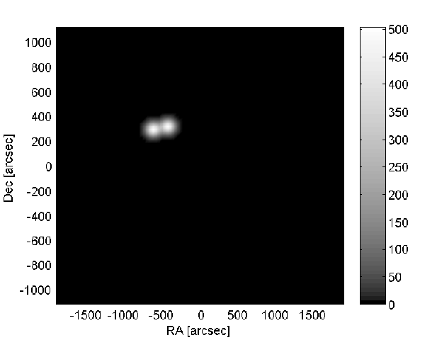
The first scenario is depicted in Figure 1. The original image consists of two closely spaced sources. Their intensities are equal and the noise was very weak, so that the image noise was 250,000 times weaker than each source. It is shown that LS-MVI succeeds in separating the two sources whilst the CLEAN method does not. Moreover, the intensities are more accurate in the LS-MVI’s image. Note that in this case the MVDR dirty image and the AAR dirty image are quite similar.


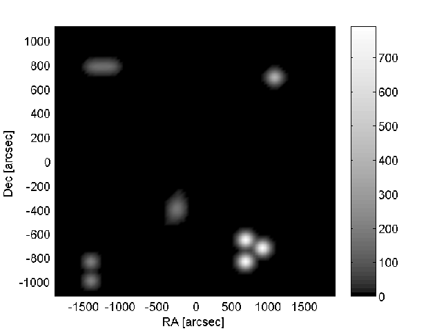
The second scenario is depicted in Figure 2. The original image consists of many sources with different intensities Fig:2(a). The intensities ratio between the strongest source and the weakest source is 16dB. The weakest source contributed to each baseline power that is equal to of the noise standard deviation on the baseline. For the WSRT this is equivalent to a source of 8 mJy when using 160 MHz band and integrating over 256 correlation lags 33 3 Based on the WSRT noise exposure calculator http://www.astron.nl/ oosterlo/expCalc.html, and using the fact that the simulated beam is of size approximately 4 pixels. As can be seen, LS-MVI performs better than CLEAN. The latter cannot differentiate between close sources, and the structures of its sources are less accurate. Moreover, LS-MVI gives better intensities estimations than CLEAN. The reason for that is the isotropic noise spectrum, that prevents direction dependent noise effects. Thus the sources intensities estimations are more accurate when based on the AAR dirty image, rather than on the conventional dirty image or on the MVDR dirty image.


The third experiment included an extended source containing a central weak point source and two extended radio lobes. The correlation matrices were generated such that the contribution of the weak source to each baseline was of the noise on the baseline. The figure presents the original image, the CLEAN image and the LS-MVI using the AAR dirty image. The CLEAN is presented after 100 and 120 iterations while the LS-MVI is presented after 100 and 300 iterations respectively. Each contour is of the dynamic range of the image. We can clearly see that the CLEAN develops a fake source a little bit below the right lobe after 120 iteration. This causes complete divergence if the CLEAN iterations are continued. On the other hand, the LS-MVI with its better power estimate can continue with many more iterations, without affecting the image.


Finally to demonstrate the improved power estimate, we have taken a cross section of the images near the center. Figure 4 presents the results, for the original image, the CLEAN after 100 iterations and the LS-MVI after 100 iterations. We can clearly see the improved power estimate.

V-B Bias of the 2D MVDR DOA estimator’s simulation
In this section we present a simulation of the bias of the 2D MVDR DOA estimator with a moving array. We have used the same array as in the previous simulations. The artificial sky image was composed of two point sources with different intensities (the weak source had power that was half of the power of the strong source). The sources contribution to each baseline was approximately 14 and 28 of the noise on the baseline. The MVDR dirty image (Def. III.1) was created based on these correlation matrices. First we found the location of the maximum intensity in the MVDR dirty image. Then we used a 2-D quadratic interpolation in order to obtain a fine 2-D MVDR location estimate. We averaged the estimates over 100 independent trials.We compared our results to the analytical expressions given in Theorem IV.1. This experiment was repeated 40 times with various angular separation of the sources. Figure 5 depicts the simulated bias () against the analytical bias, as a function of the angular distance between the two sources in l coordinates. It can be seen that the analytical results are in good agreement with the simulation results. Moreover, as the distance between the two sources increases, the bias of the estimator decreases, as expected. As the distance is larger, the influence of the sidelobes of one source on the other is smaller. The change in the bias is not monotonic in the angular separation, since the weak source moves through the sidelobes of the strong source.

VI Conclusions
In this paper we extend the matrix formulation of [5] to non co-planar arrays and polarimetric measurements. Then we propose a new parametric imaging technique that improves the resolution and sensitivity over the classical CLEAN algorithm. The method is based on several improvements: A new type of dirty image, LS estimation of the powers and semi-definite constraints. We show how the technique can be combined into self-calibration using semi-definite programming. Our semi-definite self-calibration algorithm also provides a new approach to robust beamforming with a moving array, extending the techniques of [40], [41] and [42]. We provide statistical analysis of the location estimator. Simulated examples comparing full deconvolution using LS-MVI and comparing them to the CLEAN method are presented. These simulations demonstrate that the parametric approach has higher resolution, is more robust to source structures, and performs better in noisy situations. The great potential of the methods proposed in this paper is a first step, towards the development of more advanced imaging techniques, capable of providing higher dynamic range and interference immunity as required by the radio telescopes of the future.
References
- [1] P.J. Hall, ed., The Square Kilometer Array: An Engineering Perspective. Springer, 2005. Reprinted from Experimental Astronomy Vol.17, 1-3, 2004.
- [2] J.D. Bregman, “LOFAR approaching the critical design review,” in Proceedings of the XXVIIIth General Assembly of the URSI, 2005.
- [3] G.E. Moore, “Cramming more components onto integrated circuits,” Electronics, vol. 38, Apr. 1965.
- [4] S. Boyd and L. Vandenberghe, Convex optimization. Cambridge University Press, 2004.
- [5] A. Leshem and A.J. van der Veen, “Radio-astronomical imaging in the presence of strong radio interference,” IEEE Trans. on Information Theory, Special issue on information theoretic imaging, pp. 1730–1747, 2000.
- [6] A. Leshem, A.J. van der Veen, and A. J. Boonstra, “Multichannel interference mitigation techniques in radio-astronomy,” The Astrophysical Journal Supplements, pp. 355–373, 2000.
- [7] A.R. Thompson, J.M. Moran, and G.W. Swenson, eds., Interferometry and Synthesis in Radio astronomy. John Wiley and Sons, 1986.
- [8] J.L. Yen, “Image reconstruction in synthesis radio telescopes,” in Array Signal Processing (S. Haykin, ed.), Prentice-Hall Signal Processing Series, 1985.
- [9] G.B. Taylor, C.L. Carilli, and R.A. Perley, Synthesis Imaging in Radio-Astronomy. Astronomical Society of the Pacific, 1999.
- [10] K.I. Kellerman and J.M. Moran, “The development of high resolution imaging in radio-astronomy,” Annual review of of Astronomy and Astrophysics, vol. 39, pp. 457–509, 2001.
- [11] R.J. Sault and T.A. Oosterloo, “Imaging algorithms in radio-interferometry. arxiv 070117v1..” 2007.
- [12] M. Ryle, “A new radio interferometer and its application to the observation of weak stars,” Proc. Royal Society A, vol. 211, pp. 351–375, 1952.
- [13] M. Ryle, “The new Cambridge radio telescope,” Nature, vol. 194, pp. 517–518, 1962.
- [14] J.A. Hogbom, “Aperture synthesis with non-regular distribution of interferometer baselines,” Astronomy and Astrophysics Supp., vol. 15, pp. 417–426, 1974.
- [15] U.J. Schwarz, “Mathematical-statistical description of the iterative beam removing technique (method CLEAN),” Astronomy and Astrophysics, vol. 65, pp. 345–356, 1978.
- [16] U.J. Schwarz, “The method CLEAN - use missuse and variations,” in Image formation from coherence functions in astronomy (C. van Schoonveld, ed.), pp. 261–275, 1979.
- [17] S.M. Tan, “An analysis of the properties of CLEAN and smoothness stabilized CLEAN — some warnings,” Month. Not. R. Astr. Soc., vol. 220, pp. 971–1001, 1986.
- [18] B.G. Clark, “An efficient implementation of the algorithm CLEAN,” Astron. Astrophys., pp. 377–378, 1980.
- [19] F.R. Schwab, “Relaxing the isoplanatism assumption in self-calibration: applications to low-frequency radio interferometry,” Astronomical Journal, vol. 89, no. 1, pp. 1076–1081, 1984.
- [20] Jian Li and P. Stoica, “Efficient mixed-spectrum estimation with applications to target feature extraction,” IEEE Transactions on Signal Processing, vol. 44, pp. 281–295, Feb 1996.
- [21] E.T. Jaynes Physics Review, vol. 106, p. 620, 1957.
- [22] B.R. Frieden, “Restoring with maximum likelihood and maximum entropy,” Journal of the Optical Society of America, vol. 62, pp. 511–518, 1972.
- [23] S.F. Gull and G.J. Skilling, “Image reconstruction from incomplete and noisy data,” Nature, vol. 272, pp. 686–690, 1978.
- [24] J.G. Ables, “Maximum entropy spectral analysis,” Astronomy and Astrophysics Supp., vol. 15, pp. 383–393, 1974.
- [25] S.J. Wernecke, “Two dimensional maximum entropy reconstruction of radio brightness,” Radio Science, vol. 12, pp. 831–844, 1977.
- [26] J.A. Roberts, ed., Indirect imaging. Cambridge university press, 1984.
- [27] D. S. Briggs, High fidelity deconvolution of moderately resolved sources. PhD thesis, The new Mexico Institute of Mining and Technology, Socorro, New Mexico, 1995.
- [28] A. Zeira and B. Friedlander, “Direction finding with time varying arrays,” IEEE Trans. Signal Processing, vol. 43, pp. 927–937, Apr. 1995.
- [29] B. Friedlander and A. Zeira, “Eigenstructure based algorithms for direction finding with time varying arrays,” IEEE Trans. on Aerospace and Electronic System, vol. 32, pp. 689–700, Apr. 1996.
- [30] J. Sheinvald, M. Wax, and A.J. Weiss, “Localization of multiple sources using moving arrays,” IEEE trans. on Signal Processing, vol. 46, pp. 2736–2743, Oct. 1998.
- [31] A.D. Lanterman, “Statistical imaging in radio astronomy via expectation-maximization of structured covariance matrices,” in Model-Based Image and Signal Processing, in honor of Donald L. Snyder’s 65th birthday (J.A. O’Sullivan, ed.), Springer-Verlag, In preparation.
- [32] J.E. Noordam and A.G. de Bruyn, “High dynamic range mapping of radio sources, with application to 3C84,” Nature, vol. 299, pp. 597–600, 1982.
- [33] T.J. Pearson and A.C.S. Readhead, “Image formation by self-calibration in radio astronomy,” Annual Rev. Astronomy and Astrophysics, vol. 22, pp. 97–130, 1984.
- [34] G.B. Borgiotti and L.J. Kaplan, “Supperresolution of uncorrelated interference sources by using adaptive array techniques,” IEEE Trans. on Antennas and Propagation, vol. 27, pp. 842–845, 1979.
- [35] J.D. Bregman J.P. Hamaker and R.J. Sault, “Understanding radio polarimetry: I. Mathematical foundations,” Astronomy and Astrophysics Supplement, pp. 137–147, 1996.
- [36] J.P. Hamaker, “Understanding radio polarimetry IV: The full-coherency analogue of scalar self-calibration: Self-alignment, dynamic range and polarimetric fidelity,” ASTRONOMY and ASTROPHYSICS SUPPLEMENT SERIES, vol. 143, pp. 515–534, May 2000.
- [37] J. Capon, “High resolution frequency-wavenumber spectrum analysis,” Proceedings of the IEEE, pp. 1408–1418, 1969.
- [38] A.J. van der Veen, A. Leshem, and A.J. Boonstra, “Array signal processing in radio-astronomy,” Experimental Astronomy, 2004.
- [39] P. Stoica, Z. Wang, and J. Li, “Robust Capon beamforming,” IEEE Signal Processing Letters, vol. 10, pp. 172–175, Jun. 2003.
- [40] J. Li, P. Stoica, and Z. Wang, “On robust Capon beamforming and diagonal loading,” IEEE Tran. on Signal Processing, vol. 51, pp. 1702–1715, Jul. 2003.
- [41] S.A. Vorobyov, A.B. Gershman, and Z.-Q. Luo, “Robust adaptive beamforming using worst-case performance optimization: A solution to the signal mismatch problem,” IEEE Tran. on Signal Processing, vol. 51, pp. 313–324, Feb. 2003.
- [42] R.G. Lorenz and S.P. Boyd, “Robust minimum variance beamforming,” IEEE Tran. on Signal Processing, vol. 53, pp. 1684–1696, May 2005.
- [43] S. Verdu and H. Poor, “On minimax robustness: A general approach and applications,” Information Theory, IEEE Transactions on, vol. 30, no. 2, pp. 328–340, Mar 1984.
- [44] D.H. Johnson and D.E. Dudgeon, Array Signal Processing. Prentice-Hall Inc.
- [45] D. Rieken and D. Fuhrmann, “Generalizing MUSIC and MVDR for multiple noncoherent arrays,” IEEE Trans. on Signal Processing, vol. 52, pp. 2396–2406, Sept. 2004.
- [46] M.A. Voronkov and M.H. Wieringa, “The Cotton-Schwab CLEAN at ultra-high dynamic range,” Experimental Astronomy, no. 13, pp. 13–29, 2004.
- [47] L. Vandenberghe and S. Boyd, “Semidefinite programming,” SIAM Review, vol. 38, pp. 49–95, Mar. 1996.
- [48] J. Li, P. Stoica, and Z. Wang, “Doubly constrained robust Capon beamformer,” Signal Processing, IEEE Transactions on [see also Acoustics, Speech, and Signal Processing, IEEE Transactions on], vol. 52, pp. 2407–2423, Sept. 2004.
- [49] M. Hawkes and A. Nehorai, “Acoustic vector-sensor beamforming and Capon direction estimation,” IEEE Trans. on Signal Processing, vol. 46, pp. 2291–2304, Sept. 1998.
- [50] C. Vaidyanathan and K. M. Buckley, “Performance analysis of the MVDR spatial spectrum estimator,” IEEE Trans. on Signal Processing, June 1995.
VII Appendix
In this section we derive approximate expressions for the asymptotic bias by using a first-order Taylor series expansion of and around . To reduce the notational load we present the derivation of the single covariance matrix case. In the multiple covariance matrices case is replaced by a sum and each expression can be replaced by the appropriate sum over . The final results in theorem IV.1 includes the adjustment to multiple covariance matrices. Note that is a fixed parameter representing the true covariance matrix, since we discuss only the asymptotic term. Let be fixed. The expansions around is given by:
| (59) |
and
| (60) |
Since by definition is the minimum of
Hence,
| (61) |
Proving that and using Cramer’s rule, we obtain Eqs. (49) (for k=1).
For simplicity, from now on we will denote
by .
Let us now derive the expressions for the derivatives of
.
| (62) |
Therefore,
| (63) |
where
| (64) |
Using the fact is Hermitian and simple algebraic manipulation yields
Therefore,
| (65) |
Using Eq. (65), Eq. (63) becomes
| (66) |
where we have used the fact that both and are Hermitian, and are defined in Eq. (55) for k=1. Thus we get Eq. (50) (for k=1). Similarly we derive Eq. (51).
To calculate (Eq. (52)), define as
| (67) |
Then,
| (68) |
and
Therefore,
| (69) |
Using again the fact that both and are Hermitian, we get
| (70) |
where , , and are defined in Eq. (55) for k=1. Thus we get Eq. (52) for k=1. Eq. (53) may be derived in the same way.
After some simple algebraic manipulations we get Eq. (54) for k=1. Note that is continuous, as long as does not vanish. Indeed and is positive definite (since is positive definite), so . Therefore, is continuous. Similarly, is continuous. Hence, . This completes our proof.