Mass transfer variation in the outburst model of dwarf novae and soft X-ray transients
Abstract
Context. In the standard formulation of the disc instability model for soft X-ray transient and dwarf nova outbursts, the mass transfer rate from the secondary is assumed to be constant. This may seem natural since the point remains shielded from the accretion luminosity by the accretion disc. However an indirect heating could take place and could lead to an enhancement of the mass transfer rate. It is still debated whether such an enhancement of the mass transfer rate during outbursts is a missing ingredient of the current model.
Aims. We discuss two mechanisms that could result in an enhancement of the mass transfer rate during outbursts: the hot outer disc rim itself could significantly heat the point; scattered radiation by optically thin outflowing matter could also heat significantly. We determine quantitatively the increase of the mass transfer rate resulting from an extra heating.
Methods. We estimate the heating of the point by the disc rim by analytical and numerical arguments. The fraction of the luminosity scattered by matter above the disc, here modeled as a spherically symmetric outflow, is determined analytically. We finally solve in a numerical way the vertical structure equations for the secondary star and calculate the mass transfer enhancement.
Results. During outbursts, the temperature at the outer edge of the disc reaches K. The disc edge heats up the upper layer of the secondary with a flux of the order of the intrinsic stellar flux. This probably has no large effect on the mass transfer rate. In soft X-ray transients, the environing medium of the disc (corona+wind) could back-scatter a certain fraction of the accretion luminosity toward . In dwarf novae, the same effect could be due to the wind present during outburst. Since soft X-ray transients reach high luminosities, even a low efficiency of this effect could yield a significant heating of , whereas we show that in dwarf novae this effect is negligible. Initially the incoming radiation does not penetrate below the photosphere of the secondary. Depending on the heating efficiency, which has to be determined, the mass transfer rate could be significantly increased.
Key Words.
accretion, accretion disks - binaries: close - novae, cataclysmic variables - stars: dwarf novae1 Introduction
Dwarf novae (DNe) and Soft X-ray transients (SXTs) are semi-detached binary systems that undergo regular outbursts. SXTs in outbursts reach luminosities of order of erg.s-1 in the soft X-ray band, whereas they are faint X-ray sources during quiescence (with luminosities erg.s-1). Their outbursts last for a few months and have a recurrence time in the range 1 – 50 years (Lewin et al., 1997, see). DNe are magnitude brighter during outbursts than in quiescence. Their outbursts last for a few days and recur every few weeks (Warner, 2003, see). In both types of systems, a compact object (i.e. a white dwarf in DNe and a neutrons star/black hole in SXTs) accretes from a low mass secondary star via an accretion disc. It is now believed that DNe and SXTs outbursts are both due to a thermal/viscous instability of the accretion disc triggered when hydrogen becomes partially ionized (Osaki, 1996; Lasota, 2001, see). In this picture, the accretion disc performs a limit cycle between a cold, quiescent state of low accretion rate and a hot, viscous state of high accretion rate corresponding to the outburst. The difference between DNe and SXTs timescales is thought to be due both to the irradiation of the disc by the central source in SXTs (King & Ritter, 1998; Dubus et al., 2001, see), and to a higher primary mass.
| Model | System | (h) | (K) | (1016 g.s-1) | (1016 g.s-1) | |||||
|---|---|---|---|---|---|---|---|---|---|---|
| 1 | OY Car | 1.51 | 0.6 | 0.21 | 0.1 | 0.085 | 2500 | 0.5 | 16 | 0.06 |
| 2 | U Gem | 4.24 | 1.48 | 0.29 | 0.36 | 0.7 | 3500 | 5,10 | 100 | 0.09 |
| 3 | Z Cam | 6.96 | 2.17 | 0.35 | 0.6 | 0.7 | 4200 | 30,60 | 250 | 0.1 |
| 4 | A 0620 | 7.8 | 3.9 | 0.21 | 0.1 | 0.7 | 3000 | 0.5 | 0.1 |
The thermal/viscous instability alone is not sufficient to explain the rich and diverse features of DNs and SXTs lightcurves. For example, Osaki (1989) suggested that a tidal instability driving the disc eccentric (Whitehurst, 1988, see) would account for the superoutburst phenomenon of SU UMa stars (a subclass of DNe) when coupled to the standard thermal/viscous instability. Tidal effects have also been proposed to account for the secondary maximum often present in SXTs lightcurves (Truss et al., 2002, see).
In its most common formulation, the disc instability model (DIM) assumes that the mass transfer rate from the secondary is fixed, and given by the secular losses of angular momentum from the binary system. This assumption is most likely to be wrong and significant deviation of the mass transfer rate from its secular mean on time scales as short as the outburst duration could be an essential ingredient missing in the standard model. Numerical investigations showed that variations of the mass transfer rate could explain the outburst bimodality of DNe (Smak, 1999) and that it could lead to long outbursts similar to superoutbursts (Hameury, 2000). Augusteijn et al. (1993) and Chen et al. (1993) sought to explain the rebrightenings of SXTs lightcurves by an increase of the mass transfer rate. However, in these works either an empirical relationship between the mass transfer rate and the mass accretion rate was assumed or mass transfer burst episodes were imposed without physical grounds. It has been often argued that a such mass transfer enhancement could result from irradiation of the secondary during an outburst. Viallet & Hameury (2007) investigated this problem and found that, because the point is shielded from direct irradiation disc by the secondary star, the increase of the mass transfer rate is modest.
In this paper, we investigate two different mechanisms that could be responsible for a mass transfer enhancement, resulting in both cases from an increase of the temperature at the point. Since lies in the shadow cast by the accretion disc, any heating must be indirect. The first effect that we consider is heating by radiation emitted by the hot edge of the disc during an outburst, which produces a flux at comparable to the intrinsic stellar flux. The second effect that we consider is the heating of by the accretion luminosity scattered by a wind and/or a corona extending above the accretion disc. The scattered fraction is small, but the scattered flux is still significant in SXTs due to their high luminosity in outburst. We then turn to the determination of the mass transfer enhancement. First, we compute the vertical structure of the secondary envelope in DNe and SXTs both in quiescence and outbursts to determine the dependence of the mass transfer rate versus a given incoming heating flux. Our results show that can potentially be raised by a factor of up to in SXTs, and up to in DNe. We then discuss if the effects investigated here could lead to an efficient heating of the point. This is done by computing the fraction of the incoming radiation that penetrates the photosphere. This depends on the nature of the radiation, hence on its origin. We show that the thermal flux emitted by the edge of the disc can penetrate below the photosphere of the secondary. The resulting heating is probably too small to have any major effect. For soft X-ray transients, the backscattered radiation is in the soft X-ray band and is therefore strongly absorbed by the initially neutral hydrogen in the very upper part of the atmosphere. However, this large X-ray flux significantly affects the atmosphere. A full analysis of the radiative transfer should be undertaken to determine the exact structure of the atmosphere.
The paper is organized as follow: in Section 2, we discuss the two mechanisms mentioned above. Section 3 is devoted to the computation of the vertical structure of secondary stars in DNe and SXTs, and to the relationship between the mass transfer enhancement and the heating of . Concluding remarks are given in section 4.
2 Heating flux at the point during outburst
In the following, we considere 4 models, with parameters given in Table 1, that are representative of various DNe subclasses and SXT outbursts. Models 1-3 correspond to dwarf novae with increasing orbital periods, and model 4 corresponds to A 0620-00, emblematic of short period soft X-ray transients.
2.1 Heating by the disc rim
During an outburst, the disc grows as a consequence of an effective outward transport of angular momentum. The maximum disc size is determined by tidal interactions with the secondary which effectively truncate the disc at a mean radius (Smak, 2002; Ichikawa & Osaki, 1994, see). During an outburst, the disc will reach this maximal radius, for SU UMa systems this would be true only during superoutbursts (Osaki, 1989; Osaki, 1996, see), and tidal dissipation heats up the outer region of the disc. Smak (2002) argued that tidal dissipation occurs in a very narrow region at the disc rim and suggested that this energy is radiated away by the disc edge, whereas heat generated by viscous dissipation is radiated by the surface of the disc; this contrasts with our previous work, where tidal dissipation was considered to occur on a relatively large area of the disc, significantly larger than the disc thickness (Buat-Ménard et al., 2001; Hameury & Lasota, 2005, see). We do not discuss this issue further here and we use Smak’s assumption which maximizes the energy radiated by the disc edge. We show below that, even in this very favorable hypothesis, the effect is small.
In this picture, removal of angular momentum by the tidal torque is negligible inside the truncation radius. The only effect of the tidal torque is to prevent the disc from exceeding the radius . In this prescription for tidal effects, the only free parameter is .


In the following, we determine whether can be significantly heated by the hot edge of the disc. We consider this effect only for dwarf novae, since for soft X-ray transients the major effect in heating is due to scattering by a hot corona or an outflowing wind (see the next subsection). As in Smak (2002), we first determine the tidal torque applied to the disc by the secondary, equal to the rate at which angular momentum is removed from the disc. The work done by this torque is radiated as a “tidal luminosity" , where is the Keplerian angular velocity at the disc edge. is assumed to be radiated by the disc edge, whose effective temperature is then given by:
| (1) |
where is the disc outer radius and the ratio at the outer radius appears explicitly. is the full geometrical disc thickness, of the order of a few times the vertical scale height.
Smak (2002) considered the steady state case, which made the determination of easy. As we are interested in during an outburst, we consider instead the local balance of angular momentum at the disc edge: once the disc has reached its maximal radius, the angular momentum transported at the disc edge has to be fully removed by the tidal torque. Using the standard conservation laws for angular momentum and mass, this yields:
| (2) |
where and are respectively the specific angular momentum at the outer disc edge and the specific angular momentum carried by the stream. The first term on the right hand side includes the viscous torque at the outer radius, i.e. the rate at which angular momentum is transported outwards by viscosity, and the effect of the incoming stream ( is the mass transfer rate). We use the numerical code of Hameury et al. (1998) to calculate the time evolution of the accretion disc and thus determine . The code has been modified to account for the different prescription for the outer disc radius. When , we use the free outer radius conditions (Eqs. 7, 8 in Hameury et al. 1998, note that Eq. 8 is equivalent to ). When reaches , the code switches to a fixed outer radius condition . Eq. (2) is then nonzero and yields the rate of angular momentum removal by the tidal torque without the need for tidal terms in the equations. The code switches back to the free outer radius conditions when falls below an arbitrarily small, given value. We do not include here any heating of the outer disc region due to the impact of the incoming stream (Smak, 2002, see discussion in).
Figure 1 shows the results for models 1 (left panel) and 2 (right panel). In our model 1, the disc always fills its tidal radius. Outbursts are of the inside-out type and heating fronts propagate over only of the disc. The heating front then dies out in the outer part of the disc and the corresponding outward transport of angular momentum is large enough to counteract the effect of the incoming stream. This contrasts with the normal tidal torque prescription model (as described for example in Hameury et al. 1998), where the outer radius of the disc is found to vary by about ; the reason is that the disc is too large – despite the short orbital period – given the strength of the outbursts that cannot reach the outermost parts of the disc. In Fig. 1, one can also see that the edge of the disc is heated for a longer time than the outburst duration. The effective temperature of disc edge is maximum during outburst and reaches K. For model 2, the disc outer radius varies, and the disc reaches its tidal radius during outburst. The effective temperature of the edge reaches a maximum of 1.3 K during the outburst. Note that in order to obtain a sequence of regular outbursts for this model, we used a mass transfer rate of g.s -1; for a value half the size, we obtain an irregular sequence of outbursts, having the same maximum effective temperature at the disc edge. Results for model 3 are very similar to those of model 2.
Assuming that is radiated as a blackbody, the specific intensity of the radiation (integrated over frequency) at the disc edge is:
| (3) |
Let be the solid angle subtended by the edge of the disc at the point; neglecting limb darkening and since the intensity Eq. 3 is isotropic, the point receives an incoming flux from the disc edge. The computation of is implemented in our code and is performed during the time evolution of the disc. The ratio , where is the intrinsic stellar flux, is given in Table 2. is equal to a few times the intrinsic stellar flux.
| Model | (K) | |
|---|---|---|
| 1 | 9000 | 2 |
| 2 | 13000 | 5 |
| 3 | 10000 | 2.5 |
As Smak (2002) emphasized, the assumption that tidal dissipation is radiated entirely at the edge breaks down when becomes too different from , the effective temperature at the surface of the disc due to viscous heating. In this case, one expects an inward radial heat flux, lowering and increasing . The effective temperature at the surface of the disc (at the outer radius) is shown with a dashed line in Fig. 1. One can see that the “viscous temperature" at the outer radius remains much lower than the “tidal temperature". Our determination of is therefore probably overestimated.
Since the secondary cannot occult the disc completely, an enhancement of the disc edge luminosity should be detectable during eclipses of high inclination systems. Shafter & Misselt (2006) analyzed eclipse profiles of the classical nova V Per. In this system, the accretion disc is in a hot steady state and extends to its tidal radius. Only model profiles with a hot disc rim ( K) allowed the authors to find the radial temperature profile expected in the steady state case. This range of temperature is in agreement with the tidal heating at the outer edge. In their model, the authors have for the first time taken into account the disc thickness which is crucial in determining the temperature of the disc edge. In previous studies of eclipse profiles of dwarf novae, see e.g. Bruch et al. 1996 (OY Car) and Horne & Cook 1985 (Z Cha), the disc was assumed to be “flat" (negligible thickness), which prevented a correct determination of the temperature at the disc edge.
2.2 Heating by scattering of the accretion flux
2.2.1 The dwarf nova case: scattering by a wind
The observation of UV lines with typical P Cyg profiles during dwarf novae outbursts implies the presence of mass loss in a wind (Warner, 2003, see). Under the assumption of spherical symmetry of the wind, detailed studies of the line profiles have shown that the wind acceleration is slow ; the velocity profile can be taken as (Drew, 1987; Mauche & Raymond, 1987):
| (4) |
with , yielding a slow acceleration. As in Mauche & Raymond (1987), we take cm s-1 (we will show that this parameter is of no importance in our case) and cm s-1, which is of the order of the escape velocity of the white dwarf.
Photoionisation models of the wind are consistent with a mass loss rate in the range , which translates into a few percent of the accretion rate (Hoare & Drew, 1993).
Due to the presence of matter above the disc, a fraction of the accretion luminosity is scattered toward and could contribute to its heating.
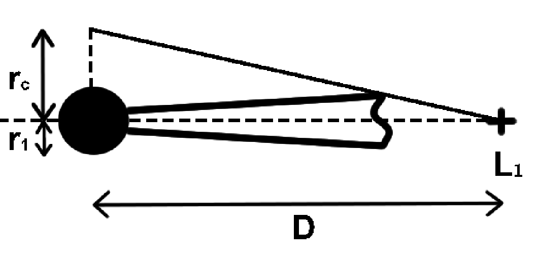
We assume in the following that of the accretion rate is lost in a spherically symmetric wind. The mass conservation law yields:
| (5) |
where is the accretion rate onto the compact object during an outburst (see Table 1), is the mass loss and is the distance to the primary center of mass. From equation 5 we deduce the radial density profile of the wind.
We consider for simplicity a uniform and isotropic opacity (corresponding to Thompson scattering by free electrons); the optical depth of the wind is then:
| (6) |
where is the total column density of the wind. The value of for models is shown in Table 3. is low and the wind is optically thin. Consequently only a very small fraction of the accretion luminosity is scattered toward . In order to determine this fraction, we suppose that no “double scattering" occurs and we neglect the radial decrease of the accretion luminosity due to scattering losses. Scattering is handled as an emissivity equal to:
| (7) |
where is the distance to the primary center of mass. The flux reflected toward is then:
| (8) |
where is the distance between and the running point . We show in the appendix that:
| (9) |
where is a geometrical weight function for the spherical shell at radius . Note that the radial integration starts at (see Fig. 2), and not at . This approximately takes into account the screening of the inner region of the wind by the edge of the accretion disc. is computed by considering that the disc has its maximal radius (see previous section) and typical ratio at the edge, see Table 1. Note that due to this screening, the value in Eq. 4, which controls the mass density of the wind near the white dwarf, does not influence the fraction that is back-scattered. However, it does influence the value of and hence , so the values of given in Table 3 should be taken with care.
Equation 9 is numerically computed with the appropriate profile. In the case of a direct illumination, the point would receive a flux equal to . As shown in Table 3, the fraction of this flux scattered toward is very small, of the order of . This yields a very low ratio. DNe have a insufficient luminosity for this effect to be significant.
| Model | |||
|---|---|---|---|
| 1 | 0.01 | ||
| 2 | 0.1 | ||
| 3 | 0.3 |
2.2.2 The X-ray transient case: scattering by a corona
Observational evidence for an accretion disc corona in low mass X-ray binaries (LMXBs) was first discussed by White & Holt (1982) and McClintock et al. (1982). The principal indicator of an extended region of hot, ionized gas above the disc is the evidence of partial eclipses of X-ray emission in high inclination systems. While the compact object is screened from the observer, a fraction as high as of the X-ray flux is left during eclipses. These sources are the so-called “coronal sources". Such a corona is believed to be present in many, if not all, LMXBs. X-ray transients in outbursts should not be an exception.
We discuss here the possibility that, during an outburst, the point receives some fraction of the accretion flux due to back-scattering by the corona.
The geometry of the accretion disc corona is still poorly understood. One can grossly distinguish between two types of geometry: a slab corona which consists of two slabs of optically thin plasma sandwiching the accretion disc or a spherical corona located around the compact object.
Let us consider first a spherical corona. With typical X-ray transient parameters (see Table 1), the value of (see figure 2) is cm. According to studies of eclipse light-curves of coronal sources, the most extended coronae are found in the brightest sources ( erg s-1) and have a radius of cm (Church & Bałucińska-Church, 2004, see). Such a corona can be screened by the accretion disc and would not scatter radiation toward .
A slab corona results from the X-ray heating of the accretion disc surface by the central source. The heated gas forms a tenuous layer with a thickness exceeding that of the disc. Begelman et al. (1983) analyzed the structure and dynamics of the X-ray heated disc. They found that, in addition to the formation of the corona, X-ray heating could also drive a thermal wind in the outer region of the disc. A slab corona could back-scatter radiation coming from the central part of the disc over the disc rim, toward the point. A wind emitted from the outer region of the disc would also contribute to this effect. It is however hard to obtain a quantitative measure of this effect.
Results obtained in the study of irradiation of the accretion disc in X-ray transients can give us a clue about the efficiency. Dubus et al. (1999) show that self-consistant computation of the radial structure of irradiated discs in SXTs leads to a problem: the disc has a convex shape and the outer, unstable, regions are screened from irradiation. This is contrary to observation and the authors replace the usual formula for the irradiation temperature in the disc (Shakura & Syunyaev, 1973, see e.g.) by the following prescription:
| (10) |
where is taken to be constant, which is thought to reflect the fact that the disc receives some X-ray flux at each radius. This could be due to warping of the disc, or to the presence of a corona. In SXT, is an adequate value (Dubus et al., 1999; Dubus et al., 2001, see). Note that a warping of the disc in its outer regions could allow a direct irradiation of . If the corona is responsible for the overall heating of the disc, could serve as a first estimate for the efficiency of the heating of the point by the corona. The flux impinging the region would therefore be:
| (11) |
where is the distance between and the compact object. SXT outbursts have typical luminosities that translate into an irradiation flux at the secondary of the order of . With , Eq. 11 yields which is very significant. This value is most probably overestimated ; a better determination, relying on a model for the corona and/or the wind, should be sought.
3 Variation of
3.1 Vertical structure in quiescence
The mass transfer rate is given by (Lubow & Shu, 1975, see):
| (12) |
where is the isothermal speed of sound which depends on the temperature at , :
| (13) |
and is the cross section of the stream (Lubow & Shu, 1975):
| (14) |
where depends only slightly on the mass ratio . Here we take , valid for in the range within 10 %.
In order to determine when an incident flux heats the upper layer of the atmosphere, we first compute the structure of the envelope of the secondary during quiescence for models by solving the standard equations:
| (15) | |||
| (16) | |||
| (17) |
where is either the radiative temperature gradient when is less than the adiabatic value with
| (18) |
where is the radiative pressure, or the convective value when the radiative gradient is superadiabatic (), calculated in the mixing-length prescription as described in Paczyński (1969). The equation of state and opacities are computed in the same way as in Hameury (1991). We use the diffusion approximation for the radiative flux, which is not accurate in optically thin regions. The true radiative flux should be computed by solving the radiative transfer, a task which is beyond the scope of the present exploratory work. The photosphere of the atmosphere is defined to be the location where , where is the Rossland optical depth.
We solve numerically Eqs. (15-17) assuming a given and at the point. is chosen so that the temperature of the model at the photosphere is equal to the value of given in Table 1. The value of is then determined from Eq. (12) with the appropriate value of and with the secular mean value of given in Table 1. The computation starts at the point and goes inward until a temperature K is reached. The Roche geometry is taken into account by using the Roche potential in the hydrostatic equilibrium equation.

Figure 3 shows the vertical structure of the secondary envelope for DNe below the period gap (model 1), DNe above the period gap (model 2 & 3) and SXTs (model 4). As seen in Fig. 3, the point lies in the radiative part of the atmosphere in the SXT case and in the convective part of the atmosphere in DNe secondaries. In each case, the point is located above the photosphere, with in model 4, in model 1&2 and in model 3 ( is the vertical pressure scale height of the envelope). This difference is due to the fact that SXTs have lower mass transfer rates than DNe, which is possible since the critical mass transfer rate above which the instability disappears is lower in an irradiated disc than in the unirradiated case (Dubus et al., 1999, see).
Figure 3 also shows that for DNe below the period gap, the temperature increases very slowly with depth in the secondary envelope. This is due to the low value of the adiabatic gradient () in the regions of molecular hydrogen dissociation present in the envelope of these low temperature stars. For DNe above the period gap, the secondary is hotter and the point lies in a region where hydrogen is neutral. As a consequence, the adiabatic gradient is larger () and the temperature increases rapidly with depth.
3.2 Vertical structure during an outburst
We now assume that an heating flux strikes the region and is absorbed below the photosphere. heats up the secondary on the thermal time scale of the atmosphere, short compared to the duration of outbursts, until the envelope reaches an outward flux equal to:
| (19) |
Here is the effective temperature of the secondary in quiescence and is the bolometric albedo that accounts for a horizontal transport of the deposited energy, which could be important in the case of deep convective stars (for radiative stars , see e.g. Smith 1995). Since its value is not known precisely, we adopt in all cases (Brett & Smith, 1993, see). It is not clear whether on the time scale of an outburst an efficient horizontal heat transport can set in.


The evolution of the subphotospheric layers has been determined by Hameury et al. (1988). As energy is deposited in sub-photospheric regions, heat diffuses inward and hinders the escape of the intrinsic stellar flux. An isothermal layer of temperature form, on top of matter that has not yet been heated. This heated layer ultimately extends to the depth where the quiescent temperature profile is equal to . However, assuming that the layer has been heated entirely by the stellar flux, its depth is restricted by the requirement that:
| (20) |
where is the duration of the outburst and is the thermal content of the layer; we take here for models and for model . We then solve Eqs. (15–17) to determine the density profile of the isothermal layer, and the new mass transfer rate is then found from (Eq. 12) with the new values of and .

Examples of models where the heating flux is are shown in figure 4. The figure shows that in this case, the isothermal layer extends down to a column density of the order of g cm-2 in dwarf novae and g cm-2 in soft X-ray transients. The depth of the layer is lower in dwarf novae because of the restriction (20) in low period systems (SU UMa) and because of the location where is quickly reached in longer period systems (U Gem and Z Cam).
The mass transfer enhancement is computed for a heating flux ranging from to . The results are shown in Fig. 5. As can be seen, the mass transfer rate enhancement is quite significant in SXTs (factor of 2 for ) and is potentially very significant (factor of 100 for ). In comparison, the mass transfer enhancement is moderate in DNe. This is a direct consequence of the different depths reached by the isothermal layer.
3.3 Absorption of the incident radiation by the secondary atmosphere
The effect of an incident flux on the secondary atmosphere depends on the spectrum of the incoming radiation, and hence on its origin. The flux absorbed below the photosphere, denoted in the last subsection, can be quite different from the incident flux . In the case of heating of by the hot edge of the disc, the spectrum of the impinging radiation can be aproximated by a blackbody spectrum with effective temperature K. In the case of heating by scattering of the accretion luminosity, we assume for simplicity that no reprocessing occurs. As one half of the accretion luminosity is emitted in the accretion disc and the other half is emitted in the boundary layer, we use two separate contributions to the energy spectrum of the incident radiation. The boundary layer emission is assumed to be a black-body ; Table 4 shows the wavelength of the emission peak for each model. For the disc emission, we use a standard multi black-body spectrum of a steady disc, in which we have taken into account the irradiation by the central source in the case of SXTs. Steady state is a very reasonable assumption for discs during outburst.
| Model | Disc edge at K | Disc | Boundary layer | ||
|---|---|---|---|---|---|
| (nm) | quiescence | ||||
| 1 | 0.25 | 0.01 | 50 | ||
| 2, 3 | 0.18 | 0.05 | 30 | ||
| 4 | 0.22 | 0.1 | 1 | ||
Radiation absorbed in optically thin layers contributes to the formation of a hot corona above the photosphere ; only the incoming radiation that penetrates below the photosphere contributes to changing the vertical structure and hence increasing the mass transfer rate. We use the ATLAS 12 code to compute the monochromatic opacities in the envelope and determine which fraction reaches the photosphere. The ATLAS 12 opacities extend from m down to 10 nm, which is a suitable range for our purpose except for the SXT case where the bulk of the accretion flux is emitted in the soft X-ray band (emission peak at nm). In this last case, the opacity is extrapolated down to very short wavelengths and includes Thomson scattering. Both continuous and line opacities of ATLAS 12 are described in Castelli (2005). Since we consider here stars with effective temperatures below 5000 K, molecular opacities are also included.
Figure 6 shows the monochromatic opacity at the photosphere of model 2. The opacity profiles of the other models show qualitatively the same behavior, the most important common feature being the very high opacity below nm due to neutral hydrogen.
We define the monochromatic optical depth :
| (21) |
We start at with an incident specific intensity (black-body of temperature ) and we compute the specific intensity at each depth that results from absorption:
| (22) |
Finally at the photosphere (depth ) we compute the fraction of energy left:
| (23) |
The results are shown in Table 4. For the radiation coming from the disc edge, approximately % of the flux is able to penetrate below the photosphere.
The radiation emitted by the boundary layer is almost completely absorbed above the photosphere of the secondary. This is because the black-body maximum is located below the Lyman limit ( nm) and absorption by neutral hydrogen is very important. This point was already discussed by King (1989) in the context of cataclysmic variables. Between and of the radiation emitted by the accretion disc reaches the photosphere. This is because the outer region of the accretion disc emits at lower energy than the boundary layer, i.e. above nm. One can check that the flux left at the photosphere is mainly in the optical and near infra-red bands.
Note however that our computation here is oversimplified since we do not consider at all the alteration of the atmosphere by the incoming radiation.
We have also computed using heated profiles we constructed in Sect 3.2. Our results show that the column density of the photosphere decreases with an increasing heating. As a consequence, an increasing fraction can be absorbed below the photosphere. Table 4 shows the fraction of the incident flux absorbed in the unperturbed atmosphere of the secondary, and that absorbed in an atmosphere efficiently heated with . We do not discuss changes for dwarf novae, since the scattered flux is far too small to have any effect. However, model 4 shows a huge difference: in quiescence nothing reaches the photospheric level whereas in the heated state, the photospheric level is so close to that most of the incoming flux reaches the photosphere. We therefore cannot deduce from such simple arguments whether the heating could be efficient or not. To obtain a quantitative result, one needs to solve the full radiative transfer problem. This is left for a future investigation.

4 Conclusion
We have considered two mechanisms that could be responsible for heating of the point during outbursts of dwarf novae and soft X-ray transients. First, the outer edge of the disc is heated by tidal dissipation and reaches an effective temperature of the order of K (see Sect. 1). We have shown in Sect. 3 that a significant part of the resulting thermal radiation can penetrate below the photosphere of the secondary. The disc edge is able to heat the upper layer of the secondary with an incoming flux comparable to the intrinsic stellar flux. This has probably no significant effect in dwarf novae. In soft X-ray transients, the dominant effect could be a heating by scattered radiation. A disc corona, or a wind driven by the X-ray heating of the disc, could act as a scattering medium, allowing the radiation to overcome the screening by the accretion disc. It is hard however to infer a quantitative estimate of this effect. However, the luminosity of SXTs are so high that even a low efficiency () could lead to a significant heating. However, the bulk of this radiation is absorbed by neutral hydrogen, and initially nothing reaches the photospheric level of the secondary star. Nevertheless, the flux is so strong that the incident radiation probably strongly modifies the state of the atmosphere. Yet it is hard to assess whether in this case an efficient heating takes place or not. The resolution of the corresponding radiative transfer should be undertaken.
In Sect. 3 we determined the relation between the mass transfer enhancement and a given heating flux impinging the point (independently of the origin of this heating). We computed the vertical structure of the secondary with the assumption of hydrostatic equilibrium. The atmosphere is not hydrostatic near the point due to the mass outflow in this region. However, departure from hydrostatic equilibrium is likely to be important only in the near vicinity of the point. We found that the point lies higher in the atmosphere in soft X-ray transients than in dwarf novae. This is a consequence of a lower value of the mass transfer rate in soft X-ray transients, where the point lies in a nearly isothermal, radiative region of the atmosphere, whereas in dwarf novae the point lies in the convective part of the atmosphere, where temperature increases more rapidly with depth. As a consequence, an incident flux can heat a significant layer in soft X-ray transients, which yields a large enhancement of the mass transfer rate. On the other hand, in dwarf novae only a narrower region of the atmosphere is affected. For a dwarf nova below the period gap, the envelope is too massive to be fully affected on the time scale of an outburst. Our results suggest that the mass transfer enhancement could be potentially very important for soft X-ray transients, up to a factor of for a heating flux equal to . For dwarf novae, the mass transfer rate enhancement is more moderate, of a factor of for a heating flux equal to . In dwarf novae, none of the effects investigated here is able to produce such fluxes. The soft X-ray transient case needs further investigation, on one hand to determine the fraction of radiation that is back-scattered toward , and on the other hand the efficiency of the heating of the secondary has to be determined properly.
Acknowledgements.
We gratefully thank Irit Idan for her help with the ATLAS 12 opacities. We thank the anonymous referee for very useful comments that helped us to improve the paper.References
- Augusteijn et al. (1993) Augusteijn, T., Kuulkers, E., & Shaham, J. 1993, A&A, 279, L13
- Begelman et al. (1983) Begelman, M. C., McKee, C. F., & Shields, G. A. 1983, ApJ, 271, 70
- Brett & Smith (1993) Brett, J. M. & Smith, R. C. 1993, MNRAS, 264, 641
- Bruch et al. (1996) Bruch, A., Beele, D., & Baptista, R. 1996, A&A, 306, 151
- Buat-Ménard et al. (2001) Buat-Ménard, V., Hameury, J.-M., & Lasota, J.-P. 2001, A&A, 366, 612
- Castelli (2005) Castelli, F. 2005, Memorie della Societa Astronomica Italiana Supplement, 8, 25
- Chen et al. (1993) Chen, W., Livio, M., & Gehrels, N. 1993, ApJ, 408, L5
- Church & Bałucińska-Church (2004) Church, M. J. & Bałucińska-Church, M. 2004, MNRAS, 348, 955
- Drew (1987) Drew, J. E. 1987, MNRAS, 224, 595
- Dubus et al. (2001) Dubus, G., Hameury, J.-M., & Lasota, J.-P. 2001, A&A, 373, 251
- Dubus et al. (1999) Dubus, G., Lasota, J.-P., Hameury, J.-M., & Charles, P. 1999, MNRAS, 303, 139
- Hameury (1991) Hameury, J. M. 1991, A&A, 243, 419
- Hameury (2000) Hameury, J.-M. 2000, New Astronomy Review, 44, 15
- Hameury et al. (1986) Hameury, J. M., King, A. R., & Lasota, J. P. 1986, A&A, 162, 71
- Hameury & Lasota (2005) Hameury, J.-M. & Lasota, J.-P. 2005, A&A, 443, 283
- Hameury et al. (1988) Hameury, J. M., Lasota, J. P., & King, A. R. 1988, A&A, 192, 187
- Hameury et al. (1998) Hameury, J.-M., Menou, K., Dubus, G., Lasota, J.-P., & Hure, J.-M. 1998, MNRAS, 298, 1048
- Hoare & Drew (1993) Hoare, M. G. & Drew, J. E. 1993, MNRAS, 260, 647
- Horne & Cook (1985) Horne, K. & Cook, M. C. 1985, MNRAS, 214, 307
- Ichikawa & Osaki (1994) Ichikawa, S. & Osaki, Y. 1994, PASJ, 46, 621
- King (1989) King, A. R. 1989, MNRAS, 241, 365
- King & Ritter (1998) King, A. R. & Ritter, H. 1998, MNRAS, 293, L42
- Lasota (2001) Lasota, J.-P. 2001, New Astronomy Review, 45, 449
- Lewin et al. (1997) Lewin, W. H. G., van Paradijs, J., & van den Heuvel, E. P. J. 1997, X-ray Binaries (X-ray Binaries, Edited by Walter H. G. Lewin and Jan van Paradijs and Edward P. J. van den Heuvel, pp. 674. ISBN 0521599342. Cambridge, UK: Cambridge University Press, January 1997.)
- Lubow & Shu (1975) Lubow, S. H. & Shu, F. H. 1975, ApJ, 198, 383
- Mauche & Raymond (1987) Mauche, C. W. & Raymond, J. C. 1987, ApJ, 323, 690
- McClintock et al. (1982) McClintock, J. E., London, R. A., Bond, H. E., & Grauer, A. D. 1982, ApJ, 258, 245
- Osaki (1989) Osaki, Y. 1989, PASJ, 41, 1005
- Osaki (1996) Osaki, Y. 1996, PASP, 108, 39
- Paczyński (1969) Paczyński, B. 1969, Acta Astronomica, 19, 1
- Shafter & Misselt (2006) Shafter, A. W. & Misselt, K. A. 2006, ApJ, 644, 1104
- Shakura & Syunyaev (1973) Shakura, N. I. & Syunyaev, R. A. 1973, A&A, 24, 337
- Smak (1999) Smak, J. 1999, Acta Astronomica, 49, 383
- Smak (2002) Smak, J. 2002, Acta Astronomica, 52, 263
- Smak (2004) Smak, J. 2004, Acta Astronomica, 54, 181
- Smith (1995) Smith, B. C. 1995, in Astronomical Society of the Pacific Conference Series, Vol. 85, Magnetic Cataclysmic Variables, ed. D. A. H. Buckley & B. Warner, 417–+
- Truss et al. (2002) Truss, M. R., Wynn, G. A., Murray, J. R., & King, A. R. 2002, MNRAS, 337, 1329
- Viallet & Hameury (2007) Viallet, M. & Hameury, J.-M. 2007, A&A, 475, 597
- Warner (2003) Warner, B. 2003, Cataclysmic Variable Stars (Cataclysmic Variable Stars, by Brian Warner, pp. 592. ISBN 052154209X. Cambridge, UK: Cambridge University Press, September 2003.)
- White & Holt (1982) White, N. E. & Holt, S. S. 1982, ApJ, 257, 318
- Whitehurst (1988) Whitehurst, R. 1988, MNRAS, 232, 35
Appendix A Derivation of Eq. 9
We give here the detailed computation of the integral:
| (24) |
with
| (25) |
We adopt a spherical system of coordinates centered on the primary center of mass, with the colatitude coordinate defined to be the angle between the running point and the line joining the primary center of mass to and with longitude coordinate . Due to the symmetry of the problem, the integral 24 becomes:
| (26) | |||||
with and . Note that the radial integration starts at (see Fig. 2) and not this approximately accounts for the shielding of the scattering region by the disc rim. The double integral involving the angular variables gives:
| (27) |
It is useful to look at the asymptotic behavior of this function: one can check that as and that as . Note that this quantity diverges at , however the integral Eq. 26 is well defined because the divergence of the logarithm function at the origin is integrable.