Heavy Quark Potential at Finite Temperature Using the Holographic Correspondence
Abstract
We revisit the calculation of a heavy quark potential in supersymmetric Yang-Mills theory at finite temperature using the AdS/CFT correspondence. As is widely known, the potential calculated in the pioneering works of Rey et al. [1] and Brandhuber et al. [2] is zero for separation distances between the quark and the anti-quark above a certain critical separation, at which the potential has a kink. We point out that by analytically continuing the string configurations into the complex plane, and using a slightly different renormalization subtraction, one obtains a smooth non-zero (negative definite) potential without a kink. The obtained potential also has a non-zero imaginary (absorptive) part for separations . Most importantly at large separations the real part of the potential does not exhibit the exponential Debye falloff expected from perturbation theory and instead falls off as a power law, proportional to for .
pacs
11.10.Wx, 11.25.Tq, 12.38MhHeavy quark potential is a very important quantity in gauge theories at finite temperature. It also has a great phenomenological relevance in connection with experimental programs in heavy ion collisions at the Relativistic Heavy Ion Collider and at the upcoming Large Hadron Collider. The melting of heavy mesons in a medium is considered to be one of the main experimental signatures for Quark-Gluon Plasma formation, the ultimate goal of such experiments. Current analyses of available experimental data indicate that the matter formed in such collisions is strongly coupled. Thus, the study of heavy quark potential requires strong-coupling techniques, such as the Anti-de Sitter space/conformal field theory (AdS/CFT) correspondence [3, 4, 5, 6]. The main goal of this work is to improve the current description of heavy quark potential at finite temperature in the AdS/CFT framework.
Until recently heavy quark potential has been calculated either analytically at small coupling using the perturbation theory, or numerically using lattice simulations. With the advent of AdS/CFT correspondence [3, 4, 5, 6], it became possible to analytically calculate the heavy quark potential at strong coupling, albeit only for the supersymmetric Yang-Mills (SYM) theory.
The first calculation of a heavy quark potential in vacuum for SYM theory was carried out by Maldacena in [7]. Soon after [7] calculations of the heavy quark potential for SYM theory at finite temperature appeared in [1, 2]. In [7] the heavy quark potential is obtained from the expectation value of a static temporal Wilson loop and in [1, 2] from the correlator of two Polyakov loops. They are calculated by extremizing the world-sheet of an open string attached to the quark and anti-quark located at the edge of the AdS5 space in the background of the empty AdS5 space in [7] and in the background of the AdS5 black hole metric in [1, 2].
The zero-temperature heavy quark potential obtained in [7] is of Coulomb type due to conformal invariance of SYM theory:
| (1) |
with the ’t Hooft coupling and . Here is the distance between the quark and the anti-quark in the boundary gauge theory.
The finite-temperature heavy quark potential obtained in [1, 2] starts out at small being close to the vacuum potential of Eq. (1), but rises steeper than the vacuum potential, becoming zero at a separation . For larger separations, i.e., for , the authors of [1, 2] argue that the string “melts”, and the dominant configuration corresponds to two straight strings stretching from the quark and the anti-quark down to the black hole horizon. The resulting potential is thus zero for and has a kink (a discontinuity in its derivative) at .
To clarify the definition of the heavy quark potential at finite temperature T let us first define the Polyakov loop for gauge theory at spatial location by
| (2) |
with the Euclidean time and . The connected correlator of two Polyakov loops can be written as [9, 8]
| (3) |
Eq. (3) is the definition of singlet and adjoint potentials in Euclidean time formalism. With the appropriate modification of Eq. (2), Eq. (3) also applies to SYM.
To calculate the Polyakov loop correlator in AdS space one follows the standard prescription outlined in [7, 1, 2] and connects open string(s) to the positions of Polyakov loops at the boundary of the AdS space in all possible ways. The two relevant configurations are shown in Fig. 1 and labeled “hanging string” and “straight strings”.
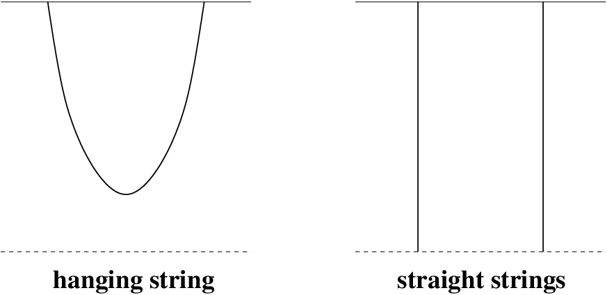
The two string configurations shown in Fig. 1 give two different saddle points of the Nambu-Goto action. In the large- large- limit the integral over all string configurations, and hence the Polyakov loop correlator as well, is equal to the sum of the contributions of the different saddle points. Actually, as was argued in [10], the two straight strings on the right of Fig. 1 have Chan-Paton labels indicating which D3 brane each string ends on. Therefore the straight strings configuration actually represents of the order of extrema corresponding to the different ways the two straight strings connect to D3 branes. Summing over all the saddle points we write (in Euclidean space)
| (4) |
with and the Nambu-Goto actions of the hanging and straight string configurations.
Comparing Eq. (4) with Eq. (3) we conclude that the hanging string configuration gives , while the two straight strings stretching to the horizon give . However itself is -suppressed and repulsive, while is of order one in -counting and attractive [8]. Renormalizing the Nambu-Goto actions in Eq. (4) by subtracting the actions of the string configurations at infinite quark–antiquark separations one obtains , which implies that is zero at leading order in . The first non-trivial contribution to is given by graviton exchanges between the strings in the bulk calculated in [10]. If exponentiated (eikonalized), they would indeed give -suppressed contributions in the exponent, as expected for . Here we will calculate the singlet potential . In lattice simulations it is usually which is understood as the heavy quark potential at finite temperature [11]. In the real-time formalism is given by the expectation value of a static (temporal) Wilson loop via
| (5) |
with the temporal extent of the Wilson loop . Note that when calculating the Wilson loop (5) in Minkowski space only the hanging string configuration contributes, as the quark and the anti-quark are projected onto a color-singlet state at initial and final times.
To find (henceforth referred to as ) we will study the behavior of the hanging string solution found in [1, 2] for . As is well-known, for the string coordinates of the solution [1, 2] become complex-valued. This simply indicates that the saddle point of the Nambu-Goto action lies in the complex string coordinate region: it does not invalidate the saddle point approximation and the results obtained with it. Similar complex-valued solutions were recently observed by the authors in [12], where the scattering amplitude of a quark–anti-quark dipole on a shock wave was calculated. In [12] the complex-valued string coordinates were instrumental for finding the unitary solution for the scattering cross section. Inspired by that example, below we will analytically continue the potential of [1, 2] into the complex region of string coordinates. The resulting potential is smooth. The corresponding force on the quarks is a continuous function of . By modifying the ultraviolet (UV) subtraction we obtain a potential which is non-zero for all separations . The potential develops an imaginary part, corresponding to the decay of the quark–anti-quark singlet state: similar results have been seen in finite temperature perturbation theory in [13, 14]. Finally, instead of Debye screening leading to exponential falloff of the potential at large distances, we find the power-law falloff at large .
We want to calculate a temporal Wilson loop in a finite-temperature SYM medium. We shall define the real-time heavy quark potential in the same way as in [13]. Following [1, 2] we start with the AdS5 black hole metric in Minkowski space [15, 3, 16]
| (6) |
where , is the coordinate describing the 5th dimension and is the curvature of the AdS5 space. The horizon of the black hole is located at with .
We want to extremize the open string worldsheet for a string attached to a static quark at and an anti-quark at . Parameterizing the static string coordinates by
| (7) |
we write the Nambu-Goto action as
| (8) |
where .
The Euler-Lagrange equation corresponding to the action (8) is
| (9) |
with . Solving Eq. (9) with the boundary conditions one gets
| (10) |
where is the Appell hypergeometric function. Here is the constant of integration corresponding to the maximum of the string coordinate along the fifth dimension of the AdS5 space, whose boundary is located at . It is given by the solution of the following equation
| (11) |
with the hypergeometric function. Indeed in the limit and Eq. (11) gives us in agreement with Maldacena’s vacuum solution [7].
The action in Eq. (8) contains a UV divergence, which has to be subtracted out. Usually, the subtraction contains a finite piece as well [7, 1, 2], which may be temperature-dependent in the case at hand. Here we will use the following subtraction, different from the one used in [1, 2]: we define the quark–anti-quark potential by
| (12) |
This subtraction insures that the real part of the potential goes to zero at infinite separations. Our subtraction (12) is consistent with that used in [7] to find the heavy quark potential at zero temperature.
Using the solution from Eq. (10) in Eqs. (8) and (12) we obtain the following expression for the heavy quark potential of the SYM theory at finite temperature:
| (13) |
Eq. (15) below is also needed to obtain Eq. (13). Our subtraction prescription resulted in the term on the right of Eq. (13) instead of , which would correspond to the subtraction done in [1, 2]. Eq. (13) along with Eq. (11) gives us the heavy quark potential as a function of the separation and temperature .
As can be readily checked numerically, given by Eq. (11) becomes complex for , leading to complex-valued and the potential . This led the authors of [1, 2] to abandon their solution for (in fact, the solution was abandoned even earlier, for ). We suggest however to interpret the complex-valued saddle points as corresponding to quasi-classical configurations in the classically forbidden region of string coordinates. This is similar to the method of complex trajectories used in quasi-classical approximations to quantum mechanics [17].
The complexification of the string coordinates simply indicates that the saddle point of the integral over string coordinates becomes complex. According to the standard AdS/CFT prescription [7], in the large- large- limit the integral over string coordinates is still dominated by the saddle point, even if it is complex. Therefore, the fact that string coordinates at the saddle point become complex does not undermine the validity of the approximation. Below we will extend the solution of Eqs. (13) and (11) to allowing for complex-valued .
First we note that the extension of the solution for following from Eq. (11) to is not unique. Two most important roots of Eq. (11) found in [1, 2] are shown in Fig. 2, which depicts real and imaginary parts of as functions of separation . There are other roots of Eq. (11) that are not shown in Fig. 2: they are either negatives of the roots in Fig. 2 or the complex conjugates of the roots in Fig. 2 and of their negatives. Such extra roots lead to physically irrelevant configurations and are not shown in Fig. 2. To determine which root gives the correct potential from first principles one has to (at least) calculate quantum corrections to the quasi-classical results shown above. While such a calculation is necessary, it would be rather tedious and is left for future work. Here we will demand that the correct root maps on the Maldacena vacuum solution [7] in the zero temperature limit. In addition we will impose unitarity to single out the right root.


Of the two roots shown in Fig. 2 only one (denoted by the solid line) maps onto Maldacena’s solution behavior of at small [7]. Since, on physical grounds, we want our potential to recover the zero temperature result [7] at small we will keep this root, and discard the other root denoted by the dash-dotted line in Fig. 2. The root given by the solid line develops a positive imaginary part for , as shown in the bottom portion of Fig. 2. As the complex conjugate of this root would also be a solution of Eq. (11), while mapping onto Maldacena’s solution for small , the question arises about the choice of one root over its complex conjugate. To select the root we note that the quantum-mechanical time-evolution operator in Minkowski metric is . Demanding that the probability of a state does not exceed one we obtain , leading to . This condition allows us to single out the solid line in Fig. 2 over its complex conjugate as the physically relevant root.


Using the solid line root of Fig. 2 in Eq. (13), we can plot the real and imaginary parts of the resulting potential. The plots are shown in Fig. 3. In the top panel of Fig. 3 we show the real part of the heavy quark potential for two non-zero temperatures, along with the zero-T curve for comparison. One can see that the non-zero temperature curves are indeed strongly screened compared to the zero temperature case, but remain non-zero at all . The subtraction scheme proposed above in Eq. (12) insures that given by Eq. (13) approaches zero at large . The use of the subtraction scheme proposed in [1, 2] would have led to going to a positive constant as .
As is clear from the lower panel in Fig. 3, the heavy quark potential develops an imaginary part for . This means the potential becomes absorptive, as the singlet state may melt in the medium. The rate of absorption increases with , as larger pairs are more likely to decay. The existence of an imaginary part in the heavy quark potential has been previously observed in perturbation theory in [13, 14]. While in Fig. 3 does not have a kink, there is a region near where the slope of the curve changes very fast. This rapid change is due to the potential developing an imaginary part, which should quickly reduce the force on the quarks.
As one can explicitly check from Eq. (13), at small we recover the zero temperature potential of [7]
| (14) |
At large separations we first use Eq. (11) to write
| (15) |
Using Eq. (15) in Eq. (13) we obtain
| (16) |
and
| (17) |
As one can see from Eq. (16), instead of the exponential falloff with characteristic of Debye screening, which would have been expected from small coupling perturbation theory and which was postulated for SYM theory at strong coupling in [10], the real part of the heavy quark potential falls off as a power, , at large . If our hypothesis of using the complex string configurations is confirmed, this would be an interesting new type of screening for the potential. However, the large negative imaginary part of the potential (17) leads to exponential decay with time of the initial (built in by construction) color correlation between the quark and the anti-quark in the Wilson loop.
Combining the large- and small- asymptotics in Eqs. (14), (16) we can interpolate the real part of the potential to write an approximate formula
| (18) |
with the new scale equal to
| (19) |
Eq. (18) fits the curves on the upper panel of Fig. 3 quite well. The parameter , defined by Eq. (18) and given in Eq. (19), can be interpreted as the screening length.
While our power-law screening is very different from the exponential falloff due to Debye screening in coordinate space, the difference is not so profound in momentum space. Define a Fourier transform of the potential
| (20) |
Using the small- asymptotics (14) one can easily show that at large the Fourier transform of the potential scales as , in agreement with the standard perturbative result. At small
| (21) |
Such asymptotic behavior is very similar to the Debye screening in the infrared (IR), given by the screened propagator in the perturbation theory with Debye mass . Hence our has qualitatively the same UV and IR asymptotics as the standard perturbative Debye-screened potential. The main difference is in the shape of at finite : unlike our is concave at all .
To summarize, we proposed a method of calculating the heavy quark potential in the finite-T strongly-coupled SYM theory in the region of separations and/or temperatures where the classical string configuration does not exist. We used an analogue of the complex trajectories method in the quasi-classical quantum mechanics [17] and analytically continued the string configurations into the region of complex coordinates. This allowed us to obtain a potential which is physically meaningful for all values of and . The potential develops an imaginary absorptive part. We would like to stress that instead of Debye screening at large separations the real part of the potential falls off as a power of the separation, which is a new and never before observed phenomenon in relativistic quantum field theories.
We would like to thank Eric Braaten, Dick Furnstahl, Andreas Karch, Samir Mathur and Larry Yaffe for informative discussions.
This research is sponsored in part by the U.S. Department of Energy under Grant No. DE-FG02-05ER41377.
References
- [1] S.-J. Rey, S. Theisen, and J.-T. Yee, Nucl. Phys. B527, 171 (1998), eprint hep-th/9803135.
- [2] A. Brandhuber, N. Itzhaki, J. Sonnenschein, and S. Yankielowicz, Phys. Lett. B434, 36 (1998), eprint hep-th/9803137.
- [3] J. M. Maldacena, Adv. Theor. Math. Phys. 2, 231 (1998a), eprint hep-th/9711200.
- [4] S. S. Gubser, I. R. Klebanov, and A. M. Polyakov, Phys. Lett. B428, 105 (1998), eprint hep-th/9802109.
- [5] E. Witten, Adv. Theor. Math. Phys. 2, 253 (1998a), eprint hep-th/9802150.
- [6] O. Aharony, S. S. Gubser, J. M. Maldacena, H. Ooguri, and Y. Oz, Phys. Rept. 323, 183 (2000), eprint hep-th/9905111.
- [7] J. M. Maldacena, Phys. Rev. Lett. 80, 4859 (1998b), eprint hep-th/9803002.
- [8] S. Nadkarni, Phys. Rev. D33, 3738 (1986).
- [9] L. D. McLerran and B. Svetitsky, Phys. Rev. D24, 450 (1981).
- [10] D. Bak, A. Karch, and L. G. Yaffe, JHEP 08, 049 (2007), eprint 0705.0994.
- [11] C. Gale and J. I. Kapusta, Finite-Temperature Field Theory (Cambridge University Press, 2006).
- [12] J. L. Albacete, Y. V. Kovchegov, and A. Taliotis (2008), eprint 0806.1484.
- [13] M. Laine, O. Philipsen, P. Romatschke, and M. Tassler, JHEP 03, 054 (2007), eprint hep-ph/0611300.
- [14] N. Brambilla, J. Ghiglieri, A. Vairo, and P. Petreczky, Phys. Rev. D78, 014017 (2008), eprint 0804.0993.
- [15] E. Witten, Adv. Theor. Math. Phys. 2, 505 (1998b), eprint hep-th/9803131.
- [16] R. A. Janik and R. Peschanski, Phys. Rev. D73, 045013 (2006), eprint hep-th/0512162.
- [17] L. D. Landau and E. M. Lifshitz, Quantum mechanics, non-relativistic theory, (Butterworth-Heinemann, 2003), vol. 3, ch. 131.