Comparison of low amplitude oscillatory shear in experimental and computational studies of model foams
Abstract
A fundamental difference between fluids and solids is their response to applied shear. Solids possess static shear moduli, while fluids do not. Complex fluids such as foams display an intermediate response to shear with nontrivial frequency-dependent shear moduli. In this manuscript, we conduct coordinated experiments and numerical simulations of model foams subjected to boundary-driven oscillatory, planar shear. Our studies are performed on bubble rafts (experiments) and the bubble model (simulations) in 2D. We focus on the low-amplitude flow regime in which T1 bubble rearrangement events do not occur, yet the system transitions from solid- to liquid-like behavior as the driving frequency is increased. In both simulations and experiments, we observe two distinct flow regimes. At low frequencies , the velocity profile of the bubbles increases linearly with distance from the stationary wall, and there is a nonzero total phase shift between the moving boundary and interior bubbles. In this frequency regime, the total phase shift scales as a power-law with . In contrast, for frequencies above a crossover frequency , the total phase shift scales linearly with the driving frequency. At even higher frequencies above a characteristic frequency , the velocity profile changes from linear to nonlinear. We fully characterize this transition from solid- to liquid-like flow behavior in both the simulations and experiments, and find qualitative and quantitative agreement for the characteristic frequencies.
pacs
05.20.Gg,05.70.Ln,83.80.IzI Introduction
Aqueous foams are collections of gas bubbles that are separated by liquid walls [1], and like other complex fluids, such as pastes, emulsions, and granular media, they exhibit transitions from solid- to liquid-like behavior in the response to applied stress or strain. For small strains, foams behave elastically with stress proportional to strain. Above the yield strain or stress, bubble rearrangements occur and the system behaves as a liquid. In contrast to Newtonian fluids, foams display complex spatio-temporal behavior in response to applied shear including intermittency, shear banding, and nonlinear velocity profiles [2, 3, 4, 5, 6, 7, 8, 9, 10, 11, 12]. Despite a number of experimental, numerical, and theoretical studies of driven foams, a fundamental understanding of the response of foam to applied shear is still lacking.
In this article, we describe a coordinated set of experimental and numerical studies of model 2D foams undergoing applied oscillatory planar shear to characterize the transition from solid- to liquid-like behavior and from linear to nonlinear velocity profiles. There have been several studies of the response of foam to steady shear, however, most of these have been performed in the Couette geometry in which flow is confined between two concentric cylinders [13]. Instead, we focus on planar shear to avoid the ‘trivial’ transition to nonlinear velocity profiles that stems from the fact that in the Couette geometry the shear stress varies with distance from the center of the shearing cell.
Another distinguishing feature of this work is its focus on oscillatory rather than steady shear as the driving mechanism. There are several reasons for selecting oscillatory shear. First, oscillatory shear allows one to control the amplitude independently from the frequency of the driving. When foams (and other complex fluids) are driven by steady shear, they exist in a highly fluidized state that is characterized by continuous, often highly correlated bubble rearrangements, or T1 events [1]. In the highly fluidized state, the statistics of T1 events determine the flow curve and control stress fluctuations [14, 15, 16, 17, 18, 19, 20, 21]. With oscillatory shear, one can study the low-amplitude flow regime in which particle rearrangement events do not occur, yet the system can transition from solid- to liquid-like behavior and from linear to nonlinear velocity profiles as the driving frequency is increased. Since T1 events can be suppressed when using oscillatory shear at low amplitude, the dissipation between fluid films becomes the dominant relaxation mechanism [22]. Thus, in this regime one can directly probe the dissipation mechanism by tuning the driving frequency.
In this article, we report on combined experiments and simulations on model 2D foams: bubble rafts in experiments [23] and the bubble model in simulations [24]. Bubble rafts consist of a single layer of bubbles floating on the surface of water. (See Fig. 1 for a snapshot of the bubble raft used in experiments.) Bubble rafts have a storied history as 2D model systems for both crystalline and disordered solids [23, 25]. In addition, we have performed a number of studies characterizing these model systems by measuring and quantifying T1 events [26], stress fluctuations [27], velocity profiles [5, 6, 7, 28, 8, 29], and flow transitions [8]. In this work, experiments on 2D bubble rafts will be compared to simulations of the 2D bubble model introduced by Durian [24]. The bubble model treats foams as soft disks that experience two pairwise forces when they overlap: a repulsive linear spring force proportional to bubble overlap and a dissipative force proportional to velocity differences between bubbles. A useful feature of the bubble model is that it can be generalized to particles with finite mass [6, 7]. Thus, the ratio of the damping and inertial forces can be varied to interrogate the damping mechanism. Recent work has shown that the bubble model successfully captures some of the features of the dynamics of bubble rafts under shear, for example, the statistics of individual T1 events [26]. Thus, a comparison of experiments of bubble rafts and simulations of the bubble model in a well-controlled planar shear geometry will allow us to further test under what conditions the bubble model accurately captures the dynamics of model foams.
We will focus on measurements of the total phase shift between the driving wall and interior bubble displacements, and velocity profiles in systems subjected to low-amplitude oscillatory planar shear. At low driving frequencies , we observe a non-zero total phase shift, while the velocity profiles rise linearly with distance from the stationary wall. At low frequencies, the total phase shift scales as a power-law with . In contrast, for frequencies above a crossover frequency , the total phase shift scales linearly with the driving frequency. At even higher driving frequencies , the velocity profiles transition from linear to nonlinear. We compare the two crossover frequencies and in the experiments and simulations and find both qualitative and quantitative agreement. The structure of the remainder of the manuscript will be organized as follows: section II, theoretical background; section III, simulation methods; section IV, experimental methods; section V, experimental and simulation results; and section VI, conclusions.
II Theoretical Background

We will now review a simple theoretical treatment of the response of an idealized viscoelastic material to an applied oscillatory strain, which will provide a framework in which to interpret the experimental and simulation results in Sec. V. The main point of this section is to identify the possible flow regimes in viscoelastic materials and their distinguishing properties. For illustration purposes, we have selected the Kelvin-Voigt linear viscoelastic model with frequency-independent elastic modulus and viscosity, though we will discuss how the results from this model can be generalized.
If a planar oscillatory shear strain is applied to a viscoelastic material (with shear along and shear gradient along ), the -displacement field of the system relative to the initial positions can be obtained by solving the force balance equation [30]:
| (1) |
where the velocity field is and is the areal mass density. The shear stress includes both the elastic and viscous contributions. As mentioned, we will focus on a linear viscoelastic material with
| (2) |
where the elastic contribution is proportional to the shear strain and the viscous contribution is proportional to the shear rate . is the elastic modulus, and is the dynamic viscosity of the material. In general, complex fluids possess complex shear moduli with arbitrary frequency dependence. We have considered this case, and find that the quantitative scaling of the crossover frequency depends on the details of the viscoelastic model. However, the qualitative features of the Kelvin-Voigt model, i.e. the existence of and , are robust.
We consider the case of parallel plates aligned along the -axis separated by a distance in the -direction as depicted in Fig. 1. The boundary at is stationary (bottom boundary), and the boundary at moves according to (top boundary). The same geometry and notation is used for the experiments and simulations. To solve Eq. 1, we use the ansatz for the displacement field. Putting these elements together, we find the following solution to Eq. 1 for the displacement field
| (3) |
and
| (4) |
for the velocity field. In Eqs. 3 and 4, the wavenumber is complex, and satisfies the dispersion relation
| (5) |
or
| (6) |
Distinctive features of the velocity profile are best described by rewriting Eq. 4 in terms of a -dependent amplitude and local phase :
| (7) |
We define the total phase shift . Because the flow is periodic, the velocity profile at a given time repeats at subsequent times separated by period . To simplify the analysis, we will focus below on velocity profiles at times when the boundary velocity is maximum ( and ). In the simulations and experiments, statistical accuracy was improved by averaging over driving cycles. We defined , where indicates an average over cycles. Monitoring the full time-dependence of the velocity profile is important, but is outside the scope of the present work. Error bars on the local phase shift and velocity profile in the simulations and experiments are given by the rms fluctuations within each bin and are typically the size of the data points in the figures unless otherwise noted.

It is instructive to consider two limits of the dispersion relation in Eq. 6: the limit of a pure solid (, ) and the limit of a pure liquid (, ). For the pure solid, we recover the dispersion relation , where is the speed of shear waves in the solid. In this case, is real, and the velocity field is a standing wave given by
| (8) |
For , , and the velocity profile becomes linear in , . For fixed system size, the transition from linear to nonlinear velocity profiles occurs when . Because is real for the case of the pure solid, the total phase shift , and the system oscillates in phase with the driving wall.
In the limit of the pure liquid, we recover the dispersion relation , where is the kinematic viscosity. In this case, with . The form of the velocity profile is more complex than that for the pure solid. However, for small driving frequencies the velocity profile can be expanded in powers of , and the first term is linear in . Thus, for or , where , the velocity profiles are approximately linear, as we found for the pure solid. However, in contrast to the pure solid, there is a non-zero total phase shift in the pure liquid since the wavenumber is complex. The full form of the phase shift is complicated, but at low driving frequencies one can expand about . For the pure liquid, at lowest order in , we find that the total phase shift scales linearly with the frequency, .

In Fig. 2, we plot the velocity profiles that satisfy Eq. 1 for two cases: (a) the pure solid ( and ) and (b) the pure liquid ( and ). In Fig. 2(a), we show that the velocity profiles for the pure solid become nonlinear when . Note that the profiles first become nonlinear by developing negative curvature above the linear profile, and then as the frequency is increased further the profile develops positive curvature below the linear profile. This nonmonotonic behavior is caused by the standing wave solution in Eq. 8. In Fig. 2(b), the velocity profile for the pure liquid begins to deviate from a linear profile when . In contrast to the pure solid, the liquid system only exhibits monotonically decaying nonlinear velocity profiles with a ‘decay length’ that decreases continuously with increasing driving frequency. An interesting feature of these profiles is that one can observe negative velocities at sufficiently high frequencies as in the case of the pure solid.
We now consider the solution to Eq. 1 for the velocity profile in the more general case of a viscoelastic material with nonzero and . In Fig. 3, we show an expanded range of driving frequencies for a viscoelastic material with , so that . Similar to the case of the pure solid, when the velocity profiles show a small negative curvature with the profile slightly above the linear profile at . At higher frequencies, the system behaves similar to the pure liquid with monotonically decaying profiles and a continuous decrease in the decay length with increasing frequency. At sufficiently high frequencies, we also observe a regime in which the velocity becomes negative. For viscoelastic materials, we define as the frequency above which the system begins to display monotonically decaying ‘liquid-like’ velocity profiles.
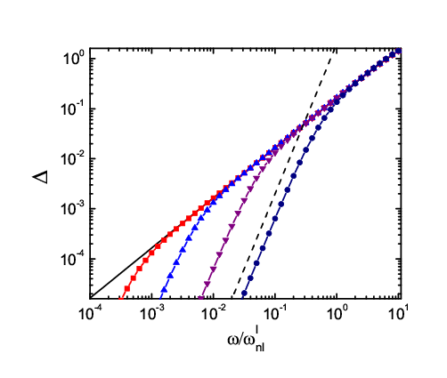
In Fig. 4, we show the total phase shift for the pure liquid and viscoelastic materials as a function of the driving frequency. (The pure solid is not shown since is identically zero for all frequencies.) As expected, for the pure liquid () scales linearly with . For viscoelastic materials with , there is a clear crossover from low-frequency scaling to high-frequency scaling with . For the Kelvin-Voigt model, the high frequency limit is equivalent to , and , corresponding to , and the low frequency limit is , corresponding to . Using these expressions, one can derive the crossover frequency explicitly, . For a more general model with a complex shear modulus, where the stress is given by , , and and are the storage and loss moduli, the values of and depend on the frequency dependence of and . However, for physically motivated , the crossover from the low-frequency elastically dominated to high-frequency viscously dominated behavior persists. One consequence of the crossover in frequency dependence is that the low-frequency total phase shift tends to zero rapidly at low frequencies, and thus may be difficult to measure at low frequencies in experiments. In our experimental studies, we were able to detect the change in scaling behavior of , but were not able to measure the scaling exponents accurately. Much more sensitive experiments are planned to measure and the storage and loss moduli at low frequencies.
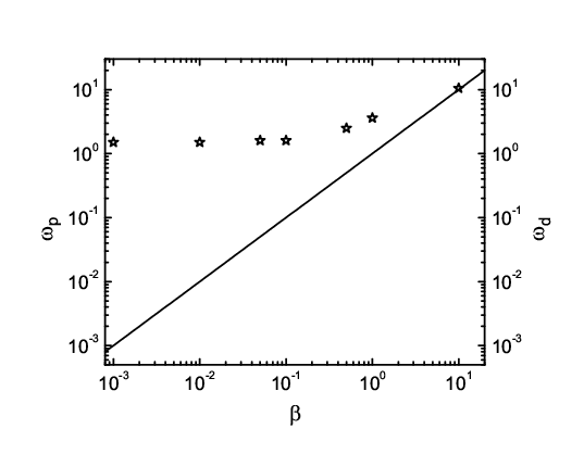
The dependence of and on for the viscoelastic Kelvin-Voigt model is given in Fig. 5. Here we used the analytical result for , but is determined numerically. This figure illustrates an important feature of the model: for , is relatively insensitive to , i.e. whether the system is solid or liquid, while decreases linearly with . Thus, as , . This is consistent with the fact that as the system becomes more solid-like, the initial deviations from nonlinearity are positive, so the transition to liquid-like behavior is delayed to higher frequencies. We expect similar behavior for more general models. By measuring these characteristic frequencies, future experimental studies will be able to characterize the material properties of foams and other complex fluids.
It is helpful to summarize the three characteristic frequencies—, , and —that were defined above. is the crossover frequency that characterizes the change in the scaling behavior of the total phase shift as a function of frequency. For pure solids, is not defined, for pure liquids, , and for viscoelastic materials . is the frequency above which we observe deviations from linear behavior in the horizontal velocity profile. For , pure liquids display decaying nonlinear velocity profiles with positive curvature, and decay more strongly with increasing frequency. In solids and viscoelastic fluids, when , the horizontal velocity profile initially possesses negative curvature with deviations ‘above’ the linear velocity profile. Thus, the curvature of the profile at low frequencies near can be used to differentiate ‘liquid-like’ from ‘solid-like’ velocity profiles. In the experiments, the solid-like response of the system at low frequencies is weak. Thus, we focus on measuring , the frequency above which the system begins to display decaying ‘liquid-like’ velocity profiles (instead of ) and in the simulations and experiments.
III Simulation Methods
We performed numerical simulations in 2D of the bubble model, which was generalized to include particles with nonzero mass , undergoing boundary-driven, oscillatory planar shear flow. The systems were composed of a total of disks with the same mass. Half of the disks were small and the other half were large with diameter ratio to avoid crystallization under shear and match the bubble distribution used in the bubble raft experiments. The original simulation cell was rectangular with -coordinates in the range and -coordinates in the range . Bubbles were initialized with random initial positions within this rectangular domain at a given packing fraction and then the system was relaxed to the nearest local potential energy minimum using conjugate gradient energy minimization [31] with periodic boundary conditions in both the and directions. All bubbles outside formed two rough, rigid boundaries. Bubbles with -coordinates in the range () formed the top (bottom) boundary. disks filled the interior of the cell between the two rigid boundaries. After the top and bottom boundaries were formed, we used periodic boundary conditions only in the -direction. Packing fractions in the range were investigated.
In the bubble model, bubble experiences two pairwise forces from neighboring bubbles that overlap : 1. repulsive linear spring forces that arise from bubble deformation
| (9) |
and 2. viscous damping forces proportional to the relative velocity between bubbles that arise from dissipation between the fluid walls
| (10) |
where sets the energy scale for elastic deformation, is the average diameter, is the center-to-center separation between bubbles and , is the unit vector that points from the center of bubble to the center of bubble , and is the damping coefficient. Note that when bubbles and do not overlap, the pairwise forces .
The ratio of the damping to inertial forces can be expressed via a dimensionless damping coefficient , where is the small bubble diameter. Underdamped (overdamped) systems are characterized by (), where for linear spring interactions. We studied both under and overdamped systems in the range . The units of energy, length, and time in the simulations are , , and , respectively.
The time evolution of the position and velocity of an interior bubble can be obtained by integrating the equation of motion
| (11) |
We employed standard Gear predictor-corrector algorithms to numerically integrate Eq. 11 for the positions and velocities of the interior bubbles [32]. This simple ‘discrete element’, short-range model for 2D foams allows us to quickly and efficiently generate an ensemble of configurations with a given set of external boundary conditions.
Oscillatory planar shear was imposed by rigidly moving all of the bubbles that comprise the top boundary in the -direction as a function of time according to
| (12) |
while bubbles that comprise the bottom boundary remain stationary. and are the amplitude and angular frequency of the sinusoidal driving. At this amplitude, we did not observe any T1 events [26] over the entire range of driving frequencies studied.

We calculated several important physical quantities in the simulations, including the phase shift of bubble -displacements relative to the motion of the boundary and the horizontal velocity profiles of the bubbles. The -displacements and velocity profiles reached steady state after a few cycles; thus, we began measurements after cycles and continued for an additional cycles to calculate averages. The height dependence of the phase shift and velocity profiles were measured by partitioning the simulation cell into equal-sized rectangular bins centered at with height large particle diameters, with measured from the bottom stationary boundary.
To calculate the local phase shift , we averaged the bubble -displacement relative to the initial position over all bubbles within the bin located at . We then fit the average bubble -displacement in each bin to to determine the local phase shift . We measured at several times during a given cycle to verify that it was time-independent, and the bubble motion was periodic. To measure the average horizontal velocity profile of the interior bubbles, we used a binning procedure identical to that employed to measure .
An important characteristic time (or frequency) scale in the bubble model is the shear rate at which the system transitions from quasistatic behavior at low shear rate (shear stress ) to highly fluidized behavior at high shear rate (, where ) when the system is driven by steady planar shear [15]. This frequency scale has also been measured in the bubble raft experiments, and thus can be used to normalize the crossover frequencies obtained in experiments and simulations. To simulate systems undergoing steady planar shear, we employed the same boundary-driven method as described above except instead of Eq. 12. The flow curve for a system with and is shown in Fig. 6, where the virial expression including dissipative forces was used to calculate the shear stress [32]. To determine , we calculated the median of the data point at which the flow curve first deviates by more than from the power-law behavior and the previous data point at higher shear rate. For the flow curve in Fig. 6, we estimate . was determined for each value of and .
IV Experimental Methods
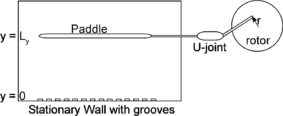
The experimental setup to apply oscillatory planar shear to bubble rafts includes three components: a rectangular basin, oscillating paddle, and imaging system. A schematic of the experimental setup is shown in Fig. 7. The basin has dimensions cm by cm and was filled to a depth of cm with a surfactant solution. A paddle was located in the middle of the basin, leaving a span of cm between it and the opposite wall. As illustrated in the schematic in Fig. 7, the ends of the system are “open” in the following sense. The entire basin is filled with bubbles, and the paddle only spans the central portion of the system. Furthermore, only the central third of the bubbles in the region covered by the paddle are used in the data analysis, and thus edge effects are minimized. The paddle was driven by an M-drive stepper motor located outside the basin. A rotor and universal (U-) joint were used to convert the axial drive of the motor into linear sinusoidal motion. The amplitude of oscillation was varied by changing the contact point between the rotor and U-joint.
The bubbles were confined between a movable paddle and a fixed wall. The bubbles were constrained to move with the paddle using metal tabs that extended one bubble diameter into the system. The tabs were spaced approximately every 5 bubbles. The fixed wall consisted of a series of square indentations approximately the size of a bubble. This fixed the bubble velocities at the stationary wall to zero. Because the first row of bubbles at each wall is interspersed with elements to hold it in place, slight distortions of the bubbles prevented accurate measurement of their positions. Therefore, in the experiments we defined the location of and to be the boundary between the first and second rows of bubbles at the stationary wall and paddle, respectively, instead of the location of the physical boundaries. For a sinusoidally oscillating paddle that is initially undisplaced, this gives the boundary condition at : , where and are the amplitude and frequency of the driving. At this amplitude, no T1 events were recorded over the entire range of .
The bubble raft consisted of a bidisperse distribution of bubble sizes: a to ratio of to diameter bubbles, which corresponds to a diameter ratio . The solution composition was 80% deionized water, 15% glycerol, and 5% miracle bubble (Imperial Toy Corp), which is a commercially available surfactant. The bubbles were produced by passing compressed nitrogen through the solution via a needle. The diameter of the needle and nitrogen pressure determine the final size of the bubbles. To create bidisperse bubble mixtures, we used two needles with different sizes at constant pressure. After the bubbles were produced, we stirred the solution with a glass rod to break-up large-scale crystalline domains so that only short-range order persisted. We tuned the pressure to prevent multiple layers of bubbles from building up in the -direction.

The definition of the gas (or liquid) area fraction for a bubble raft is somewhat imprecise because the bubbles form 3D structures on the water surface, which makes it difficult to define the amount of fluid in the walls. Also, using definitions based on T1 events present challenges because true vertices do not exist in bubble rafts, and therefore, minimum edge lengths are not well-defined. This is in contrast to fully confined two-dimensional systems, such as soap films, for which more precise definitions of liquid area fraction exist [33]. Therefore, for bubble rafts, one typically reports an operational definition of the gas area fraction, , as the average cross-sectional area of bubbles that is visible in the images. This is typically done by applying a fixed cutoff to the images to separate pixels inside and outside of the bubbles. One expects that this method will provide values for that approximate the definition of the packing fraction used in the bubble model. Using this operational definition, we find for the bubble raft experiments. The error is estimated based on a range of choices for reasonable cutoff values. As we will show, one advantage of our studies is that they can provide a method for calibrating our definition of the gas area fraction for bubble rafts with the packing fraction for the bubble model.

To visualize the bubble motions, a pixel CCD camera was held above the basin. The floor of the basin was constructed from glass, which allowed the entire bubble raft to be illuminated from below by an electroluminescent film (manufactured by Luminous Film Inc.). A frame rate of frames per second was sufficient to capture the bubble motion. The raw experimental images were filtered and thresholded to demarcate the spatial location of each bubble. Further details of the image processing are provided in Ref. [28, 29, 34].
To measure the velocity profiles, we divided the system in the -direction into equal-sized rectangular bins between and . The instantaneous velocities of bubbles were then calculated by subtracting the center of mass positions of the bubbles in consecutive image frames for each bin. We employed a PIV procedure to measure the time evolution of the bubble velocities and thus calculate the phase shift relative to the driving. The horizontal component of the velocity of the interior bubbles can be parameterized by the rms velocity , frequency of oscillation , and local phase shift with respect to the moving top boundary. The horizontal component of the velocity of the interior bubbles is therefore given by
| (13) |
where , which allows us to calculate the local phase shift relative to the moving boundary. In Sec. V below, we will show results for the total phase shift .
In the oscillatory planar shear experimental setup, we are not able to directly measure the shear stress and thus the flow curve. However, the flow curve has been measured previously for a bubble raft with similar parameters (shown in Fig. 8) [27]. We employed the same method as in the simulations to determine the crossover shear rate at which the system transitions from the quasistatic to the power-law flow regime.
V Experimental and Simulation Results

In Figs. 9 and 10, we show the results from the experiments in which bubble rafts were subjected to low amplitude oscillatory planar shear. Fig. 9 displays the horizontal velocity profiles (measured at times when the boundary velocity is maximum as defined in Sec. IV), over a range of driving frequencies. For this system, we find that the velocity profiles transition from nearly linear to ‘liquid-like’ nonlinear near . Note that at the lowest driving frequency, it appears that the velocity profile displays ‘solid-like’ behavior with slight negative curvature above a linear profile, but this feature is comparable to the size of the fluctuations. Since this feature is difficult to detect and the nonlinear liquid-like profiles are more robust in the experiments, we will focus on measurements of instead of .
In Fig. 10, we show measurements of the total phase difference between bubbles near the top and bottom boundaries as a function of the driving frequency. As discussed in Sec. II, for a viscoelastic material we expect a crossover in the scaling of the total phase difference as the driving frequency is increased. For the experiments, we were unable to fully characterize the crossover behavior due to limits in our ability to measure the phase shift at low frequencies. However, using the maximum possible values of the total phase shift at the lowest frequencies red triangles in Fig. 10, we can set a lower-limit on the exponent for the low-frequency scaling regime. This gives us a transition from , with , at low-frequencies to linear scaling at high frequencies. Thus, for the bubble raft system, we estimate , and thus .

We also performed simulations of the bubble model undergoing small amplitude oscillatory planar shear over a range of packing fractions and damping coefficients to compare to the bubble raft experiments. The trend for each set of and was similar: low frequency profiles are linear with a nonzero total phase shift followed by a transition to nonlinear liquid-like profiles when . In addition, the crossover in the scaling behavior of versus was observed. This characteristic behavior is highlighted in Figs. 11 and 12, which show the velocity profiles and total phase shift for the bubble model with and . We find and for this set of parameters. In the low-frequency limit, we find , with (blue dashed line in Fig. 12), which is similar to the scaling predicted for the Kelvin-Voigt model [35].
Figure 13 summarizes the simulation data (black squares) for the transition to liquid-like nonlinear profiles () and the crossover frequency (). We show both characteristic frequencies and at fixed as a function of including the under- and overdamped regimes and at fixed as a function of . To directly compare the results in experiments and simulations, we normalize and by obtained from the steady planar shear flow curves at each and . The experimental results are also displayed in Fig. 13; they are represented as solid lines since and are not known precisely for the bubble raft experiments. The simulations indicate that at fixed , the dependence of and is fairly weak as the dissipation switches from underdamped to overdamped. At fixed , both and increase with packing fraction, if we exclude the first point at .

VI Conclusion
We find that the bubble model captures all of the qualitative features of the response of the bubble rafts to low-amplitude oscillatory planar shear flow. The key elements of the response include: 1. A regime with linear velocity profiles, but a nonzero total phase shift at low frequencies and 2. At the highest frequencies, a regime with liquid-like nonlinear profiles and nonzero total phase shift. In addition, in the low frequency regime, there is a crossover in the scaling of total phase shift as a function of the driving frequency. The bubble model reproduces each of these distinctive features found in the bubble rafts.
The quantitative agreement shown in Fig. 13 between the simulations and the experiments is also encouraging. In the range of parameters that we expect to correspond most closely to the experiments ( and ), we find agreement to within error bars between the experiment and simulations for the characteristic frequency at which the system transitions from linear to liquid-like nonlinear velocity profiles, and , which characterizes the change in scaling of the total phase shift.
The bubble model is often used to characterize highly-fluidized flows where T1 bubble rearrangement events occur since it can quantify the statistics of these rearrangement events. It has not been employed as often to quantitatively study slow, dense flows where bubble rearrangements are rare since the results can depend on the dissipation model. One of the unique aspects of this study is that it allows a direct comparison between the bubble model and bubble raft experiments in the regime where T1 events and other large-scale bubble rearrangements do not occur, which enables stringent tests of the dissipation mechanism in the bubble model. The observed qualitative and quantitative agreement between simulation and experiment provides evidence that the bubble model provides a faithful, yet simple description of dissipation between liquid walls in bubble rafts.

Our focus on the low-amplitude oscillatory shear regime, in the absence of T1 events, provides important insights into the response of foams to applied stress. First, we find that the bubble rafts clearly exhibit dissipative behavior despite the absence of T1 events. This can only be due to motion in the fluid films, and emphasizes that further quantitative studies of film-level dissipation mechanisms are crucial to understanding foam rheology [22]. Second, studies of the response of 3D foams and emulsions to oscillatory shear suggest that there are important differences between the two systems in the low-amplitude regime [36, 37, 38]. Thus, studying the low-amplitude regime will highlight key differences in the mechanical response of a variety of soft glassy materials. Finally, in this article we presented novel results that demonstrate the existence of two additional time (or frequency) scales associated with the response of foam to applied shear: and (or ). Thus, we expect that these characteristic time scales will also play a key role in determining the flow curve and velocity profiles for foams undergoing steady planar shear flow.
A quantitative comparison between the bubble raft experiments and bubble model simulations also provides a method to calibrate the gas area-fraction of the bubble rafts, which is notoriously difficult to measure in foam experiments. Of the three frequently used quasi-two dimensional experimental setups (bubble rafts, bubble rafts with a top glass plate, and bubbles confined between two solid surfaces), it is most difficult to define the area fraction in the bubble rafts. By combining the bubble model simulations and Surface Evolver computations [39, 40], it will be possible to define an effective area fraction that will allow direct comparison between bubble raft experiments and other quasi two-dimensional glassy and jammed systems confined to surfaces and thin films. In the future, we will perform additional experiments over a range of packing fractions, surfactants that yield bubbles with varied elastic properties, and liquid viscosities to investigate whether the predictions of the simple viscoelastic model in Sec. II for the - and dependence of and are valid for the bubble rafts.
Acknowledgements.
Financial support from the Department of Energy [DE-FG02-03ED46071 (MD), DE-FG02-05ER46199 (NX), and DE-FG02-03ER46088 (NX)], NSF [DMR-0448838 (CSO) and CBET-0625149 (CSO)], and the Institute for Complex Adaptive Matter (KK) is gratefully acknowledged.References
- [1] D. Weaire and S. Hutzler, The Physics of Foams (Claredon Press, Oxford, 1999).
- [2] P. Coussot, J. S. Raynaud, F. Bertrand, P. Moucheront, J. P. Guilbaud, H. T. Huynh, S. Jarny, and D. Lesueur, Phys. Rev. Lett. 88, 218301 (2002).
- [3] F. Varnik, L. Bocquet, J.-L. Barrat, and L. Berthier, Phys. Rev. Lett. 90, 095702 (2003).
- [4] A. Kabla and G. Debrégeas, Phys. Rev. Lett. 90, 258303 (2003).
- [5] J. Lauridsen, G. Chanan, and M. Dennin, Phys. Rev. Lett. 93, 018303 (2004).
- [6] N. Xu, C. S. O’Hern, and L. Kondic, Phys. Rev. Lett. 94, 016001 (2005a).
- [7] N. Xu, C. S. O’Hern, and L. Kondic, Phys. Rev. E 72, 041504 (2005b).
- [8] C. Gilbreth, S. Sullivan, and M. Dennin, Phys. Rev. E 74, 051406 (2006).
- [9] E. Janiaud, D. Weaire, and S. Hutzler, Phys. Rev. Lett. 97, 038302 (2006).
- [10] R. J. Clancy, E. Janiaud, D. Weaire, and S. Hutzler, Eur. J. Phys. E 21, 123 (2006).
- [11] G. Katgert, M. E. Möbius, and M. van Hecke, Phys. Rev. Lett. p. accepted (2008).
- [12] A. Wyn, I. T. Davies, and S. J. Cox, Euro. Phys. J. E 26, 81 (2008).
- [13] L. D. Landau and E. M. Lifshitz, Fluid Mechanics, Second Edition : Volume 6 (Course of Theoretical Physics) (Butterworth-Heinemann, 1987).
- [14] S. Hutzler, D. Weaire, and F. Bolton, Phil. Mag. B 71, 277 (1995).
- [15] D. J. Durian, Phys. Rev. E 55, 1739 (1997).
- [16] Y. Jiang, P. J. Swart, A. Saxena, M. Asipauskas, and J. A. Glazier, Phys. Rev. E 59, 5819 (1999).
- [17] S. Tewari, D. Schiemann, D. J. Durian, C. M. Knobler, S. A. Langer, and A. J. Liu, Phys. Rev. E 60, 4385 (1999).
- [18] M. Dennin and C. M. Knobler, Phys. Rev. Lett. 78, 2485 (1997).
- [19] A. D. Gopal and D. J. Durian, Phys. Rev. Lett. 75, 2610 (1995).
- [20] M. Dennin, Phys. Rev. E 70, 041406 (2004).
- [21] T. Okuzono and K. Kawasaki, Phys. Rev. E 51, 1246 (1995).
- [22] N. D. Denkov, S. Tcholakova, K. Golemanov, K. P. Ananthapadmanabhan, and A. Lips, Phys. Rev. Lett. 100, 138301 (2008).
- [23] L. Bragg and W. M. Lomer, Proc. R. Soc. London, Ser. A 196, 171 (1949).
- [24] D. J. Durian, Phys. Rev. Lett. 75, 4780 (1995).
- [25] A. S. Argon and H. Y. Kuo, Mat. Sci. and Eng. 39, 101 (1979).
- [26] M. Lundberg, K. Krishan, N. Xu, C. S. O’Hern, and M. Dennin, Phys. Rev. E 77, 041505 (2008).
- [27] E. Pratt and M. Dennin, Phys. Rev. E 67, 051402 (2003).
- [28] Y. Wang, K. Krishan, and M. Dennin, Phys. Rev. E 73, 031401 (2006).
- [29] Y. Wang, K. Krishan, and M. Dennin, Phys. Rev. Lett. 98, 220602 (2007).
- [30] A. M. Kosevich, E. M. Lifshitz, L. D. Landau, and L. P. Pitaevskii, Theory of Elasticity: 3rd Ed., Volume 7 (Course on Theoretical Physics) (Butterworth-Heinemann, 1986).
- [31] W. H. Press, B. P. Flannery, S. A. Teukolsky, and W. T. Vetterling, Numerical Recipes in Fortran 77 (Cambridge University Press, New York, 1986).
- [32] M. P. Allen and D. J. Tildesley, Computer Simulation of Liquids (Oxford University Press, New York, 1987).
- [33] C. Raufaste, B. Dollet, S. Cox, Y. Jiang, and F. Graner, Eur. Phys. J. E 23, 217 (2007).
- [34] F. Ding, A. J. Giacomin, R. Byron, and C.-B. Kweon (1999).
- [35] In the bubble model simulations, we have performed preliminary measurements of the frequency-dependent storage and loss moduli, and . We find that the linear response regime occurs for . Despite this, we find that the scaling behavior of with frequency is consistent with the Kelvin-Voigt model.
- [36] A. Saint-Jalmes and D. J. Durian, Journal of Rheology 43, 1411 (1999).
- [37] S. Cohen-Addad, H. Hoballah, and R. Höhler, Phys. Rev. E 57, 6897 (1998).
- [38] S. A. Khan, C. A. Schnepper, and R. C. Armstrong, Journal of Rheology 32, 69 (1988).
- [39] K. A. Brakke, Phil. Trans. R. Soc. A 354, 2143 (1996).
- [40] S. J. Cox and E. Janiaud, Phil. Mag. Letts. 88, 693 (2008).