Analytical Solutions of Open String Field Theory

Journal: Physics Reports

Ehud Fuchs Email: udif@aei.mpg.de Michael Kroyter Email: mikroyt@aei.mpg.de Address: Max-Planck-Institut für Gravitationsphysik
Albert-Einstein-Institut
14476 Golm, Germany
AEI-2008-056

Abstract

In this work we review Schnabl’s construction of the tachyon vacuum solution to bosonic covariant open string field theory and the results that followed.

We survey the state of the art of string field theory research preceding this construction focusing on Sen’s conjectures and the results obtained using level truncation methods.

The tachyon vacuum solution can be described in various ways. We describe its geometric representation using wedge states, its formal algebraic representation as a pure-gauge solution and its oscillator representation. We also describe the analytical proofs of some of Sen’s conjectures for this solution.

The tools used in the context of the vacuum solution can be adapted to the construction of other solutions, namely various marginal deformations. We present some of the approaches used in the construction of these solutions.

The generalization of these ideas to open superstring field theory is explained in detail. We start from the exposition of the problems one faces in the construction of superstring field theory. We then present the cubic and the non-polynomial versions of superstring field theory and discuss a proposal suggesting their classical equivalence. Finally, the bosonic solutions are generalized to this case. In particular, we focus on the (somewhat surprising) generalization of the tachyon solution to the case of a theory with no tachyons.

Keywords:

String Field Theory

PACS

11.25.Sq

1 Introduction

String field theory is a field theoretical framework for string theory. As such, it can potentially be used for evaluating scattering amplitudes using Feynman diagram techniques, for studying non-perturbative effects of the theory and for exploring various string vacua by studying classical solutions.

Many attempts have been made to find analytical solutions of (open covariant bosonic) string field theory, since its introduction by Witten [1]. It took twenty years until such a solution was constructed by Schnabl [2]. This construction drew much attention and was followed by several other analytical solutions and other generalizations that improved significantly our understanding of string field theory. It is the purpose of this work to review these developments in order to make them more accessible to the general string theory community.

Previous attempts towards analytical solutions within string field theory used various tools. Among other approaches one can find:

•

Conformal field theory (CFT) methods [3, 4]: Defining the star product and integration in terms of CFT expressions enables the usage of many tools and gives a geometric picture to the problem, which can then be dealt with in various conformal frames. Moreover, many CFT methods are insensitive to the given background and are thus universal¹¹ 1 From a technical point of view, universality is the property of being dependent on the matter sector only through its energy-momentum tensor. We give more details on that in the next two sections.. Universality is an important property of solutions that represent tachyon condensation [5]. Indeed, CFT methods proved essential for the recent progress.
•

Half-string formalism [6, 7, 8, 9, 10]: A fundamental entity in the construction of string field theory is the star product, which can be cast into a form analogous to a matrix product, with the two halves of the string playing the roles of the two matrix indices. Bogoliubov transformation to the vacuum built upon the two string halves simplifies the form of the star product. One less favorable feature of this approach (and some of the next ones) is that it is based on a given (flat) background and is therefore not universal²² 2 Note that the basic idea of the half-string formalism can be presented in a universal way. The Bogoliubov transformation, on the other hand, refers to a specific background..
•

Simplifying the non-linear term in the equation of motion [11]: The equation of motion contains a single non-linear piece. As in the case of the Riccati equation, simplifying the form of the non-linear term has the potential of rendering the equation solvable. This approach led to the algebraic construction of the surface-state star-projector known as the sliver. The construction itself turned out to be equivalent to the half-string approach.
•

Representing the star product in a Moyal form [12, 13, 14, 15, 16, 17, 18]: A natural framework for addressing non-commutative products is the Moyal approach, which gained popularity in the string theory community following [19]. It was found that the star product can be represented as an infinite dimensional tensor product of Moyal pairs.
•

Diagonalizing the star product [20, 21]: In the oscillator basis, the star product is defined using some infinite dimensional matrices that can (almost) be simultaneously diagonalized. This results in the continuous basis (aka ${\kappa}$ -basis). This approach led to some results in the matter sector. The inclusion of the ghosts, however, turns out to be more problematic.
•

Vacuum string field theory [22, 23, 24, 25, 26, 27, 28, 29]: This is not a genuine way to solve string field theory. Instead, the form of the theory expanded around the (tachyon) solution, after an unknown (and presumably singular) field redefinition, is guessed. This approach led to numerous analytical results. However, its scope of validity and its relation to the standard string field theory were not fully clarified.
•

Identity string field based solutions [30, 31, 32, 33]: The star product contains an identity element. This state is, however, singular in several respects, e.g., it is not a normalizable state [34] and in the CFT description it represents surface gluing. Moreover, it is not killed by $c_{0}$ , which suppose to be a derivation of the star product [35], implying $0\neq c_{0}\left|1\right>=c_{0}(\left|1\right>\star\left|1\right>)=(c_{0}\left|1\right>)\star\left|1\right>+\left|1\right>\star(c_{0}\left|1\right>)=2c_{0}\left|1\right>$ , i.e., a contradiction. An advantage of the identity based solutions is that they are universal. On the other hand, while the identity based solutions are formally well defined, the problems with the identity string field rendered the evaluation of the action of these solutions ambiguous³³ 3 After the first version of this paper appeared, the papers [36, 37] appeared, which improved the credibility of the identity based solutions..
•

Using other surface states to define solutions [38, 39, 40, 41]: In order to bypass the problems with the identity string field, while keeping some of the nice properties of the solutions, one can choose to work with other star-algebra projectors, such as the butterfly and the sliver. Constructing solutions turns out to be more complicated in this case than in the case of the identity based solutions.

In this work we focus on Schnabl’s solution and the developments that followed. This construction uses ideas from most of the approaches described above. Hence, we introduce some of these tools. While we tried to make this review self-contained, the reader may want to consult also older reviews focusing on other aspects of string field theory. The following is a list of related reviews.

•

An introduction to string field theory emphasizing the Batalin-Vilkovisky (BV) approach and perturbation theory is the classical review by Thorn [42].
•

Shorter modern general introduction to string field theory can be found in [43, 44].
•

The issue of tachyon condensation in string field theory and vacuum string field theory is addressed in [45].
•

General and extensive reviews of tachyon condensation covering also other frameworks for addressing this subject are [46, 47, 48, 49, 50].
•

A short review of the early achievements following Sen’s conjectures is [51].
•

A review that describes many representations of the string field algebra with some focus on string field theory as a non-commutative field theory is [52].
•

The Moyal approach to string field theory is introduced in [53].
•

Two papers that stress the algebraic structure of the star product are [54, 55].

Let us describe the content of the various sections (by order) and their interrelations, in order to answer the perpetual question: How to use this review?

1.

In the rest of the introduction we briefly describe the advance in computing scattering amplitudes in string field theory, where impressive progress has been obtained. While this is not a result regarding analytical solutions, it is important and relevant enough to be shortly described here. We refer the reader to the original works for a complete and clear exposition of this important subject.
2.

This is an introductory section, where string field theory basics are described. Researchers familiar with its construction can skip this part.
3.

Another introductory section, in which Sen’s conjectures and their study within level truncation are described. It serves as a motivation and a historical overview and can also be skipped.
4.

Here we present some of the tools needed for the derivation of Schnabl’s solution.
5.

In this section Schnabl’s construction of the tachyon vacuum is derived using the tools of the previous section. The proofs of Sen’s conjectures for this solution are then described.
6.

This section presents some of the ways by which analytical solutions describing marginal deformations were obtained within string field theory. It relies on some basic concepts from the previous two sections.
7.

The recent advance relies mainly on CFT technics. Still, we give an oscillator description of Schnabl’s solution in this section. It relies only on some basic formulas from section 5 and the oscillator approach is explained therein. Other sections do not depend on this one and it can be skipped by readers interested in the main root of advance in the field.
8.

Here we describe the generalization of the matters presented in previous sections to open superstring field theory. The peculiar obstacles for the construction of a superstring field theory are described, as well as the superstring field theories themselves. This section relies on most of the previous ones.
9.

An outlook.

1.1 Scattering amplitudes

In string field theory scattering amplitudes can be defined even off-shell. Off-shell scattering amplitudes can be used as building blocks for loop amplitudes as well as for the evaluation of the tachyon potential. The first calculation of off-shell amplitudes was performed in [56]. The evaluation of the quartic term in the tachyon potential immediately followed [57]. This calculation was extended to higher levels and developed in [58, 59, 60] and in the Moyal approach [16, 18].

Scattering amplitudes were commonly calculated in the Siegel gauge. The attractive properties of the gauge choice introduced by Schnabl changed that. The Schnabl gauge has also some less attractive properties. It is based on an operator, which is not hermitian. It is singular in some sense and two Schwinger parameters should be used to describe a propagator instead of one [2]. Preliminary results in the Schnabl gauge were obtained in [61]. In this paper it was also suggested to use a hermitian version of Schnabl’s operator in order to fix the gauge.

The scattering amplitudes calculated in [61] seemed not to obey some expected symmetries. A careful study of the subject [62] showed that the propagator should be regularized. The results now were shown to obey some of the symmetries, while it was claimed that the other ones are peculiar to the Siegel gauge.

Up to this point, only (off-shell) tree amplitudes were considered in the Schnabl gauge. A thorough study of scattering amplitudes using a general gauge choice based on the $b$ -ghost, termed linear $b$ -gauges, was performed in [63]. Regularity conditions on the gauge choice were stated and it was found that the Schnabl gauge is located on the boundary of the regular region in the space of $b$ -coefficients. Nevertheless, no explicit problems with the results in Schnabl gauge were obtained, unlike in the case of its hermitian counterpart. Another important discovery of [63] was that Schnabl’s condition cannot be imposed at all ghost numbers. This result does not afflict previous calculations, since it is of importance only when loop amplitudes are considered, in which string fields of arbitrary ghost number appear. General $b$ -gauge choices imply different gauge conditions at different ghost numbers. Still, the question remains, whether the Schnabl gauge can be used for the evaluation of general loop amplitudes. The disturbing (and novel) property of this gauge is that it fixes the string mid-point. Thus, it may seem that moduli space cannot be covered.

This problem was addressed in [64], where the Schnabl gauge was defined as a limit of regular $b$ -gauges. A careful study of the limit showed that the limiting wedge states should be glued not in the standard way, but using a slant, which is responsible for a “hidden boundary at infinity”. The introduction of slanted wedges enabled the authors to show that at least at 1-loop level the moduli space is covered in the Schnabl gauge, despite the apparent problems. This seems as a strong evidence in favour of the possibility that Schnabl’s gauge can be used to an arbitrary loop level. Moreover, it was claimed that the results are technically much easier to derive than in the Siegel gauge. There is still work to be done, though. It would be desirable to study the general covering of moduli spaces, to calculate explicit scattering amplitudes and to address the Schnabl gauge using a BV formalism.

2 String field theory basics

String field theory is an approach to string theory, which is at least conceptually the most straightforward one. This approach generalizes the particle physics tools of second quantization to string theory. In particle physics second quantization amounts to taking the Schrödinger equation of a particle and reinterpreting it as the equation of motion of a field. It turns out that upon quantization, such a field describes just a collection of non-interacting particles of the type of the original one. To this one can add interaction terms obeying some principles, such as symmetry and renormalizability, in order to get the full field theory of interacting particles. One added advantage is that the classical equations of motion of the field can also reveal non-perturbative effects. Thus, the quantum interaction of particles and the classical, non-perturbative effects, are related.

In string theory the “first quantized” world-sheet approach already specifies the interaction in the form of the Polyakov path integral. One may hope then, that the string field theory is uniquely defined by the world-sheet theory. If this is the case, one may hope to find this string field theory and then study it both for understanding and controlling string interactions and as a tool for the study of non-perturbative effects is string theory. Indeed, already in 1990, before the big advance in understanding non-perturbative string theory following the introduction of D-branes by Polchinski [65], a numerical solution to the equations of motion of string field theory was found [66]. This solution amounts to the closed string vacuum left after the removal of a D-brane. This, however, was not understood at the time and the interpretation of the solution had to wait to the introduction of the celebrated Sen’s conjectures, to be described in section 3.

There are several perturbative string theories and one should be chosen in order to construct a string field theory. There are also several approaches for quantization on the world-sheet, e.g., light-cone. So we stress at this point that unless otherwise stated, we shall be dealing with open bosonic strings and will do so in a covariant formalism, where one can hope to gain some insight about the general symmetry structure of the theory.

At the linearized level string field theory should give the equation of motion [67, 68]

Q_{B}\Psi=0\,,

(2.1)

where $\Psi$ is the string field and $Q_{B}$ is the BRST operator on the world-sheet of the open bosonic string. One can think of the string field as a linear combination with momentum-dependent coefficients (fields) of states of the first quantized ghost number one space. Hence, it is an off-shell generalization of the vertex operator. In the usual flat space it takes the form,

\left|\Psi\right>=\int d^{26}k\Big(T(k)c_{1}+C(k)c_{0}+A_{\mu}(k)\alpha^{\mu}_{-1}c_{1}+...\Big)\!\left|k\right>,

(2.2)

with the usual definition

\left|k\right>=e^{ikX(0)}\left|0\right>.

(2.3)

The infinity of fields composing it are the momentum-dependent coefficients of the various modes. Each can be characterized by its level, that is its eigenvalue with respect to $L_{0}+1$ (ignoring the momentum part). Thus, the tachyon field $T$ is of level zero, while the photon field $A_{\mu}$ and the (auxiliary) field $C$ are of level one. The free equation of motion (2.1) should be accompanied by the free gauge transformation

\Psi\rightarrow\Psi+Q_{B}\Lambda\,.

(2.4)

Thus, the equation of motion of the string field corresponds to the condition of being closed and the gauge transformation identifies string states whose difference is exact. The gauge string field ${\Lambda}$ itself⁴⁴ 4 Throughout this manuscript we refer to ${\Lambda}$ as the “gauge string field”. This terminology might cause confusion, since in field theories, such as QED, one usually refers to $A_{\mu}$ as the “gauge field” and to ${\Lambda}$ as the “gauge parameter”. The string field $\Psi$ generalizes $A_{\mu}$ and also includes such a component field. Hence, it would have been natural to refer to $\Psi$ as the gauge string field. Nonetheless, we save this terminology for ${\Lambda}$ in order to stress that it is not a parameter, but rather a collection of infinitely many component fields. We then refer to $\Psi$ as the “physical string field”, or just as the “string field” for short. Both terminologies appear in the literature, i.e., in some papers the “gauge string field” or “gauge field” refers to ${\Lambda}$ as we do here, while in others it refers to $\Psi$ . consists of an off-shell linear combinations of states with ghost number zero. This structure resembles that of differential forms, with $Q_{B}$ playing the role of the differential, since it obeys

Q_{B}^{2}=0\,.

(2.5)

Note however, that unlike for forms in a finite dimensional space, here there are “forms” of an arbitrary integer degree, from minus infinity to infinity. The gauge transformation (2.4) is accordingly reducible at an infinite order, since a transformation of the form

\Lambda^{(n)}\rightarrow\Lambda^{(n)}+Q_{B}\Lambda^{(n-1)}\,,

(2.6)

does not contribute to the transformation of $\Lambda^{(n+1)}$ performed in the same way, due to (2.5). Here, the superscript represents the “form-degree”. Since $Q_{B}$ increases the ghost number by one, the form-degree can be identified with the (first quantization) ghost number. Being a one-form, it is natural to declare that the string field is an odd element.

An appropriate linearized action is [69]

S_{\text{lin}}=-\frac{1}{2}\left<\Psi\right|Q_{B}\left|\Psi\right>,

(2.7)

where $\left<\Psi\right|$ is the BPZ conjugate of $\left|\Psi\right>$ . Let us explain the coefficient in front of (2.7). The minus sign is needed in order to get the canonical sign for the component fields. For the tachyon field $T$ , which is the first field in the expansion (2.2), one gets

	$\displaystyle S=-$	$\displaystyle\frac{1}{2}\int d^{26}k\,d^{26}k^{\prime}\,T(k)T(k^{\prime})\left<k\right\|c_{-1}Qc_{1}\left\|k^{\prime}\right>=$		(2.8)
		$\displaystyle\frac{1}{2}\int d^{26}k\,d^{26}k^{\prime}\,T(k)T(k^{\prime})\left<k\right\|c_{-1}c_{0}c_{1}(1-k^{\prime 2})\left\|k^{\prime}\right>=\int d^{26}k\,\frac{1-k^{2}}{2}T(k)^{2}\,.$

Here we used the BPZ conjugation property of the $c$ field, as well as the oscillator expansion of $Q_{B}$ , neglecting in the intermediate step some terms that do not contribute to the inner product. We also defined $\alpha^{\prime}=1$ and used

\left<0\right|c_{-1}c_{0}c_{1}\left|0\right>=\frac{1}{2}\left<\partial^{2}c\partial cc\right>=1\,,

(2.9)

as the normalization convention in the ghost sector. Given our other convention, that of a mostly positive metric, the resulting action for the tachyon field $T$ has the canonical form and we also see that it is indeed a tachyonic field. For higher level fields one may have to adjust the coefficient in the definition of the field in order to get a canonical form. The sign is, however, canonical for all fields.

The inclusion of interactions into this formalism was performed by Witten [1]. The action is given by

S=-\int\Big(\frac{1}{2}\Psi\star Q\Psi+\frac{g_{o}}{3}\Psi\star\Psi\star\Psi\Big)\,.

(2.10)

Here $g_{o}$ is the open string coupling constant that can (at least classically) be set to unity by a field rescaling. We shall set it to unity unless otherwise stated. From (2.10), one can derive the equation of motion⁵⁵ 5 The derivation is somewhat formal at this stage. In order to be able to truly derive it, one should first specify the meaning of the operations involved and conclude that a variant of the fundamental lemma of the calculus of variations holds in this case. All that, in fact, works out well.,

Q\Psi+\Psi\star\Psi=0\,.

(2.11)

The integration, the star product and the derivation $Q$ are (bi-)linear operations over the space of (arbitrary ghost number) string fields ${\cal A}$

\int:{\cal A}\rightarrow{\mathbb{C}}\,,\qquad\star:{\cal A}\times{\cal A}\rightarrow{\cal A}\,,\qquad Q:{\cal A}\rightarrow{\cal A}\,.

(2.12)

Witten assumed that these entities obey some algebraic relations, described below. He claimed that the emergent (noncommutative geometry) structure is the natural one for describing string field theory. Regardless of this structure, the first requirement of interacting string field theory is that in the limit $g_{o}\rightarrow 0$ , it reduces to the non-interacting theory (2.7). This is the case if one identifies⁶⁶ 6 The definition of $\int\Psi_{1}\star\Psi_{2}\star\Psi_{3}$ is more involved. We return to this issue shortly.,

Q=Q_{B}\,,\qquad\int\Psi_{1}\star\Psi_{2}=\left<\Psi_{1}\vphantom{\Psi_{2}}\right|\left.\!\vphantom{\Psi_{1}}{\Psi_{2}}\right>.

(2.13)

Henceforth, $Q$ will represent the BRST operator $Q_{B}$ . Other realizations of $Q$ (denoted ${\cal Q}$ ), obeying the algebraic structure, are also of importance. A particular example is obtained when the theory (2.10) is expanded around a solution. We describe this case in section 3.

Other then linearity, Witten’s axioms state that the star product is associative and $Q$ is an odd derivation with respect to it, namely⁷⁷ 7 Throughout this paper $A$ in $(-1)^{A}$ represents the grading of $A$ .

Q^{2}=0\,,\qquad Q(A_{1}\star A_{2})=(QA_{1})\star A_{2}+(-1)^{A_{1}}A_{1}\star(QA_{2})\,,\qquad\int QA=0\,.

(2.14)

Here, $A_{1,2}$ are string fields of an arbitrary ghost number. The star product preserves the grading and the ghost number. Another axiom states that under integration the string fields behave like differential forms,

\int A_{1}\star A_{2}=(-1)^{A_{1}A_{2}}\int A_{2}\star A_{1}\,.

(2.15)

These axioms are identical to those obeyed by differential forms, except the fact that in the case of differential forms (2.15) holds even without integration⁸⁸ 8 It turns out that in the bosonic case the integral is non-zero only for a string field of ghost number three. Thus, for the bosonic string the sign factor $(-1)^{A_{1}A_{2}}$ equals unity. However, if the string fields themselves are allowed to carry Grassmann grading, the sign can become important. This is the case when the BV formalism is used in order to handle the gauge symmetry. Moreover, in the case of Berkovits’ version of superstring field theory, to be introduced in section 8.2, the total ghost number should equal two and the minus sign is important.. The action (2.10) can thus be considered as a generalization of the Chern-Simons action.

From the analogy with the Chern-Simons action we recognize that the action (2.10) is invariant under the infinitesimal gauge transformation

\delta\Psi=Q\Lambda+\Psi\star\Lambda-\Lambda\star\Psi\,,

(2.16)

where $\Lambda$ is a ghost number zero string field. This infinitesimal gauge transformation can be exponentiated to give the finite gauge transformation,

\Psi\rightarrow e^{-{\Lambda}}(Q+\Psi)e^{\Lambda}\,,

(2.17)

where multiplication, exponentiation, as well as any other function of string fields, should be performed by expanding the relevant function in a series, while keeping the order of string fields intact and using the star product for the evaluation of all products. The $1$ that is obtained at the zeroth order is realized by the identity string field, described below. No ambiguities can emerge, since the star product is the only way by which string fields can be multiplied. We continue to write it explicitly in the introductory sections, but it will be left implicit in the remaining of the paper, except in cases where its inclusion improves readability.

The gauge transformation (2.16) is reducible, since a variation of the form

\delta\Lambda=Q\Lambda_{-1}+\Psi\star\Lambda_{-1}-\Lambda_{-1}\star\Psi\,,

(2.18)

induces no change for $\Psi$ in (2.16), provided that $\Psi$ obeys the equation of motion (2.11), i.e., it is on-shell. Similarly,

\delta\Lambda_{-n}=Q\Lambda_{-(n+1)}+\Psi\star\Lambda_{-(n+1)}-\Lambda_{-(n+1)}\star\Psi\,,

(2.19)

will induce no change in $\Lambda_{-n+1}$ . This follows from

\delta^{2}A=(Q\Psi+\Psi\star\Psi)\star A-A\star(Q\Psi+\Psi\star\Psi)\,,

(2.20)

where again $A$ is a string field of an arbitrary degree. Thus, the (non-linear) gauge generator $\delta$ is nilpotent only on-shell [70], in which case the gauge system is infinitely reducible. A sensible way to deal with reducible gauge systems, as well as with gauge systems that close only on-shell, is given by the BV formalism [71, 72, 73, 74, 75] (and the reviews [76, 77]).

The BV formalism was implied for quantizing string field theory in [78, 79, 80]⁹⁹ 9 A BRST approach to string field theory was implied in [81, 82, 83] using the “mid-point light-cone gauge”.. It turns out that the infinity of ghost fields that should be added can be identified with string fields of (first-quantized) ghost number $n_{g}<1$ , while the infinity of anti-fields can be identified with string fields of ghost number $n_{g}>1$ . The identification is such that the ghost numbers of a field and its anti-field sum up to 3, i.e, the anti-field of the classical (ghost number one) string field carries ghost number two, the anti-field of the first (ghost number zero) ghost carries ghost number three and so on. As usual, the coefficient fields carry alternating parity. When this alternating parity is combined with the parity of the various ghost-number string states, it results in string fields of a fixed, odd, parity. These string fields can be summed to give (an odd) string field, whose ghost number is not constrained,

\Psi=\sum_{n=-\infty}^{\infty}\Psi_{n}\,.

(2.21)

The classical master equation is obeyed by an action, which is identical in form to (2.10), only with the string field being given by (2.21), rather than by $\Psi_{1}$ . This action can be gauge fixed by the introduction of a gauge fixing fermion. A common gauge choice is the Siegel gauge

b_{0}\Psi=0\,.

(2.22)

This is an extension of the Feynman gauge for photons, since this condition results in the Feynman gauge for the massless vector component of the string field, upon level truncation¹⁰¹⁰ 10 One can consider also other gauges, such as the analogue of the Landau gauge. A study of gauges that interpolate between the Feynman-Siegel and the Landau gauges was carried out in [84, 85]. Related discussion was given in [86]. Note, however, that there is more than one possible extension of, e.g., the Feynman gauge, for the string field. Another such extension, the Schnabl gauge, played important role in the recent developments.. In this gauge, the equation of motion (2.11) reduces to

c_{0}L_{0}\Psi+\Psi\star\Psi=0\,.

(2.23)

In order to preserve associativity, Witten suggested that the star product should implement the geometric picture of gluing the right half of the first string with the left half of the second string, while integration should amounts to gluing together both halves of the same string around the middle. This suggestion is consistent with (2.13), since in this case one gets just a gluing of two strings with their orientation reversed, i.e., the BPZ inner product [87]. With these identifications of the star product, the integral and the derivation, it was shown by Giddings et. al. that the Veneziano amplitude is reproduced from the action (2.10) and that at higher order in $g_{o}$ it reduces to the Polyakov path integral with correct covering of moduli space [88, 89, 90]. A gap in the proof of moduli space covering was filled up by Zwiebach [91].

For practical calculations it is useful to represent the star product using either CFT expressions as derived in [3, 4] or using oscillator expressions in the flat background as described in [92, 93, 94, 95, 96, 97]. The former method has the advantage of being universal. That is, it does not depend on a choice of a background, as long as it is composed of a $bc$ system coupled to a $c=26$ BCFT. Indeed, most of the recent developments in the field were achieved using this formulation. Nevertheless, the latter method has also proved useful, especially, but not only, for describing phenomena peculiar to a given background. We now turn to describe the CFT approach. We describe the oscillator method and the recent related results in section 7.

In the seminal papers [3, 4], LeClair, Peskin and Preitschopf defined more general string vertices by CFT expectation values on the disk, as

\int\Psi_{1}\star\ldots\star\Psi_{n}=\left<f^{(n)}_{1}\circ\Psi_{1}(0),\ldots,f^{(n)}_{n}\circ\Psi_{n}(0)\right>.

(2.24)

Here, the string fields on the left hand side are interpreted as operators acting on the vacuum. In the right hand side a given set of conformal transformations acts on these operators, mapping them from the upper half plane to various points on the disk, in some given canonical representation of the disk. The brackets represent the CFT expectation value of the theory living on the disk. This expectation value turns the data encoded in the insertions (the choice of the operators to be inserted $\Psi_{k}$ and the choice of mappings that implement the insertions $f_{k}^{(n)}$ ) into a number. The formalism is general. In order to reproduce Witten’s theory the conformal transformations should be fixed, such that one gets the advocated gluing. If we choose the unit disk as the canonical representative, as in figure 1, the conformal transformations take the form

f^{(n)}_{k}=\Big(\frac{1+i\xi}{1-i\xi}\Big)^{\frac{2}{n}}e^{\frac{2\pi ik}{n}}\,.

(2.25)

Note that the local coordinate patch in the upper half plane, i.e., the top half-unit-disk, is transformed under these maps to wedges with angles of $\frac{2\pi}{n}$ and these wedges are glued together such that the right half of the $k^{\text{th}}$ string is glued to the left half of the $(k+1)^{\text{th}}$ string.

Refer to caption — Figure 1: The N-vertex represented on the unit disk. Each string state is transformed to a $\frac{2\pi}{N}$ wedge and the edges of these wedges are glued to each other.

In this representation the symmetry of the vertex under cyclic permutation is manifest. Other coordinate systems can be more adequate for specific problems. We return to this point in section 4.

The CFT representation makes it clear that the $n$ -vertices are multi-linear functions. In particular, the two-vertex forms a bi-linear map, rather than a hermitian inner product, as one might have expected [98]. It is possible to impose a reality condition on the string field,

\Psi^{*}=\Psi\,.

(2.26)

The conjugation in the above equation represents a hermitian conjugation followed by the inversion of the orientation of the string. In terms of the operators producing the string state this conjugation corresponds to the composition of hermitian and BPZ conjugations. When this reality condition is imposed, the two-vertex forms also a hermitian inner product.

The CFT methods of [3, 4] can be used not only for defining string vertices, but also for defining string fields of a special class, called surface states, which will be very useful in the following sections. Surface states are generalizations of the one-vertex, in which the function $f_{1}^{(1)}$ of (2.25) is replaced by another (almost) arbitrary function $f$ . Thus, there is a 1-1 correspondence between the set of permissible functions $f$ and the set of surface states. Given $f$ , we define the surface state $\left<S\right|$ (or $\left<S_{f}\right|$ if several such states are involved) by declaring that its contraction with an arbitrary test state,

\Psi={\cal O}_{\Psi}(0)\left|0\right>,

(2.27)

obeys,

\left<S\vphantom{\Psi}\right|\left.\!\vphantom{S}{\Psi}\right>=\left<f\circ{\cal O}_{\Psi}\right>.

(2.28)

This definition might seem to be unrelated to any particular surface, as opposed to what one might expect from the term “surface state”. Nonetheless, a particular surface certainly enters this definition, as we have to specify the representation of the disk chosen for the evaluation of the CFT expectation value. One might think that this choice is immaterial, since in a CFT, expectation values are by definition invariant under reparametrization of the disk (i.e., under conformal transformations). Indeed, the representation of the disk can be modified. However, this leads also to a change of the function $f$ , which is in fact necessary for the invariance of expectation values. Hence, the function $f$ and the choice of the representation for the disk hold the same information. Surface states can, therefore, be defined either by fixing the disk (e.g., to the upper half plane) and specifying $f$ , or by fixing $f$ while specifying the surface that should be used for the evaluation of the expectation value. It is also possible to specify both, a surface $\Sigma$ and a conformal transformation $f$ . While such representations are somewhat degenerate, they might be very useful in some cases. One can write $f_{\Sigma}$ and $\left<S_{\Sigma}\right|$ , in order to stress that everything depends on the choice of the surface $\Sigma$ . Similarly, the expectation value (2.28) can be written as,

\left<S_{\Sigma}\vphantom{\Psi}\right|\left.\!\vphantom{S_{\Sigma}}{\Psi}\right>=\left<f_{\Sigma}\circ{\cal O}_{\Psi}\right>_{\Sigma}\,.

(2.29)

A nice geometric interpretation of surface states (see figure 2 $(a)$ ) can be obtained by choosing $f(z)=z$ [24]. In the BPZ picture, the inner product corresponds to the gluing of two states, which can be thought of as a state and a test state. The test state is created by the insertion of the operator ${\cal O}_{\Psi}$ at the origin, while the state itself is created by an insertion at infinity. The regions around $z=0$ and $z=\infty$ are the local coordinate patches of the two states. These two local coordinate patches meet on the half-circle $|z|=1$ and we think of the string wave functions on the curve $|z|=1$ as evolving from the insertions at $z=0,\infty$ towards this curve. The inner product is then the overlap of the wave functions of the two strings at $|z|=1$ . On the other hand, in the representation of surface states discussed above, the state is not created using an insertion at infinity. Rather, it is created by choosing a non-standard form for the local coordinate patch of the surface state itself. Of course, the surface state can also be represented in the usual manner using the insertion at infinity and both representations should lead to the same wave function at $|z|=1$ , since the test state $\Psi$ in (2.28) is arbitrary. We conclude that a surface state is a state for which the insertion that creates the state can be traded for a surface deformation. This can only be the case if the operator that creates the surface state is an operator that generates a finite surface deformation¹¹¹¹ 11 So far we are considering genuine surface state, without any further insertions. The generalization to “surface states with insertions”, which is in fact a degenerated representation of all string fields, would be described below..

Figure 2: Two possible representations of a surface state. In

(a)

, the local coordinate patch takes its canonical form, while in

(b)

, the whole surface takes a canonical form (a unit disk here, but other canonical representations, e.g., the upper half plane, are possible). It is generally impossible to find a canonical transformation in which both take their canonical form. The only exception is that of the surface state representing the

SL(2)

invariant vacuum

\left<0\right|

. It is, however, possible to fix three points of the local coordinate patch. These are most naturally chosen to be the two points of the boundary of the local coordinate patch that touch the second patch and the puncture at which the test state is to be inserted, i.e., the point

\pm 1

and

0

(a)

can be sent to

\pm 1

and

-i

(b)

(this choice can become singular for some singular surface states, e.g., the identity string field). This assignment completely fixes the local coordinates. In particular, it fixes the mid-point

M

. Then, the points

\pm 1

and

M

fix a local coordinate system also on the other patch. One can refer to the two as the local coordinate patch of the test state and the local coordinate patch of the state itself. Unfortunately, in much of the literature both are called “the local coordinate patch”, which can lead to confusion. Note, that in the representation

(a)

, a general surface state might not be represented as a simple surface in the complex plane, as it might involve a multiple cover of parts of the complex plane. This will result in cuts in this representation. This is not a problem, as long as the representation

(b)

is well defined.

This geometric picture leads also to an algebraic representation for surface states. It is known that infinitesimal deformations of a surface are obtained by the Virasoro generators. Hence, finite deformations are obtained by an exponentiation of those generators. Thus, we conclude that a general surface state can be written as,

\left|S\right>=\exp\big(\sum_{n=2}^{\infty}s_{n}L_{-n}\big)\left|0\right>,

(2.30)

where the $s_{n}$ are the coefficients defining the surface state. The simplest surface state is the vacuum, for which the conformal map is the identity map $f(z)=z$ . Using the standard local coordinate patch, while evaluating the CFT expectation value on the upper half plane, is the same as a contraction with the vacuum state. Hence, we conclude that for $\left|0\right>$ , $s_{n}=0\ \forall n$ . The relation between the coefficients $s_{n}$ and the conformal transformation $f$ in the general case was described in [99].

The form (2.30) for surface states implies that in the oscillator representation of flat space background, a surface state is a squeezed state, i.e., its matter part (we focus on one dimension for simplicity) can be represented by,

\left|S\right>=e^{\frac{1}{2}a_{n}^{\dagger}S_{nm}a_{m}^{\dagger}}\left|0\right>.

(2.31)

The matrix $S_{nm}$ can be deduced from the conformal transformation $f$ or from the coefficients $s_{n}$ . The converse, however, does not necessarily hold, namely there are many squeezed states, which are not surface states. A simple criterion for deciding whether a given (matter) squeezed state is (the matter part of) a surface state was introduced in [100]. Another criterion was later introduced that stressed integrability as the main character of surface states [101] (integrability within this context was further studied in [102, 103]). The two criteria were shown to be equivalent in [104], where it was also shown that the first column of the defining matrix of a squeezed state is equivalent to a unique surface state. Related study of the ghost sector was performed in [105, 106, 107, 104].

An important property of surface states is that a given surface defines a surface state for an arbitrary BCFT. Thus, it is possible to discuss, e.g., the sliver (a particular surface state) on a D25-brane, as well as the sliver on the D0 brane. It is also possible to study separately the matter and ghost parts of a surface state and further separate the surface state into various sectors. Note, however, that string fields that are defined by different surface states in different sectors might be inconsistent [99]. One normally thinks of “balanced”, e.g., “geometric” surface states, i.e., the Virasoro operators in (2.30) are total Virasoro operators.

Another important consequence of the representation (2.30) is that surface states are BRST closed,

Q\left|S\right>=0\,,

(2.32)

since the BRST charge commutes by construction with all the Virasoro generators. An important special case is

Q\left|1\right>=0\,,

(2.33)

where $\left|1\right>$ is the identity string field, which is a surface state by definition, since it is generated by the conformal transformation $f_{1}^{(1)}$ defining the one-vertex. The relation (2.33) is important for the consistency of Witten’s axioms, since the identity string field spans a one-dimensional subspace isomorphic to the complex numbers inside the string field algebra and “constants” should be annihilated by any derivation, $Q$ in particular.

3 Sen’s conjectures

An important advance in string field theory followed the realization that it is the ideal framework for addressing Sen’s conjectures [108, 5]. Sen’s work addressed the fate of the tachyon that is living on the bosonic D-brane¹²¹² 12 Similar conjectures hold also for the open string tachyon on a non-BPS D-brane and the tachyon living on the D-D̄ pair [109, 110, 111, 112, 113].. According to the conjectures, the tachyon describes the instability of the D-brane. An effective tachyon potential should have a local maximum around zero, where the D-brane exists. This potential should also have a local minimum¹³¹³ 13 The tachyon potential in the supersymmetric cases is bounded from below and the potential is symmetric around the origin. The bosonic potential is not symmetric and CFT analysis suggests that it is unbounded below. The “local minimum” of the tachyon potential at the non-perturbative vacuum, might well be a saddle point.. A solution in which the tachyon acquires this value as a vev (other fields also acquire vevs) represents the absence of the original D-brane¹⁴¹⁴ 14 The actual time-dependent process of tachyon condensation, was described by Sen in the “rolling tachyon” papers [114, 115]..

This picture suggests the following properties:

1.

The depth of the local minimum equals the tension of the original D-brane. This reflects the energy difference between the solutions with and without the D-brane.
2.

Other solutions exist, representing lower dimensional D-branes. These solutions are lumps from the perspective of the tachyon field.
3.

There are no perturbative states around the tachyon solution, since perturbative states in open string field theory represent open string degrees of freedom and there are no open strings when the D-brane is absent.

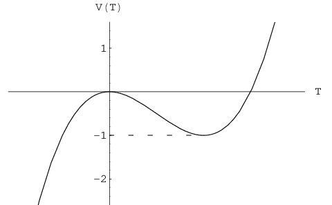
The first of Sen’s conjectures states the following. Fix the value of the tachyon field to a constant and solve the equations of motion of all the other components of the string field. The action as a function of the tachyon field should be similar to the one depicted in figure 3. The local minimum of the potential represents the solution describing the condensation of the D-brane. Thus, the action of the solution should equal minus the tension of the D-brane (with proper normalization of the space-time volume).

The second conjecture is related to the study of properties of solutions that are generally space-time dependent. For a solution to represent a lump of, e.g., co-dimension one, it has to reduce to the vacuum solution when one moves in this one dimension away from the core, which should be thin in some sense. Analogously to the first and third conjectures, the solution should have the correct tension and carry the appropriate perturbative spectrum in order to describe a D-brane of the appropriate dimension.

In order to understand the third conjecture we have to examine the form of the action (2.10) when expanded around the solution. The expansion is obtained by substituting

\Psi\rightarrow\Psi_{0}+\Psi\,,

(3.1)

into the action. As the original action is cubic it is also cubic with respect to the shifted string field. The zero order term is the constant that is used for testing the first conjecture. However, as a constant it does not contribute to the equation of motion and so can be neglected. The first order term is absent by definition, since we expand around a solution, which is an extremum of the action. The third order term cannot be changed by a shift of the field. Thus, theories that one gets by expansion around different backgrounds differ only in the form of their kinetic, i.e., second order, term. Direct evaluation gives,

S=-\int\Big(\frac{1}{2}\Psi\star{\cal Q}\Psi+\frac{1}{3}\Psi\star\Psi\star\Psi\Big).

(3.2)

The new kinetic operator is defined by its action on a string field with arbitrary ghost number $A$ by,

{\cal Q}A=QA+\Psi_{0}\star A-(-)^{A}A\star\Psi_{0}\,.

(3.3)

This form of the kinetic operator is not fixed by the ghost number one string field $\Psi$ that appears in the action. Moreover, as far as the action is concerned, we could have written the kinetic operator as ${\cal Q}\Psi=Q\Psi+2\Psi\star\Psi_{0}$ . We have to choose the symmetric form ${\cal Q}\Psi=Q\Psi+\Psi\star\Psi_{0}+\Psi_{0}\star\Psi$ in order to be able to write the equation of motion around the solution as,

{\cal Q}\Psi+\Psi\star\Psi=0\,.

(3.4)

The dependence on the parity of the form $-(-)^{A}$ appearing in (3.3) implies the derivation property of the new kinetic operator

{\cal Q}{\cal Q}A=0\quad\Longleftrightarrow\quad Q\Psi_{0}+\Psi_{0}\star\Psi_{0}=0\,.

(3.5)

This implies that the gauge symmetry written in terms of ${\cal Q}$ takes exactly the same form as when written in terms of the original $Q$ in (2.16) and (2.19).

Sen’s conjectures were addressed using several formalisms, such as effective theory analysis [116, 117, 118, 119, 120] and toy models such as p-adic string (field) theory [121, 122, 123, 124] (developed in [125, 126])¹⁵¹⁵ 15 We refer the reader to some of the reviews mentioned in the introduction for details regarding developments using other formalisms.. However, as the conjectures involve a zero-momentum tachyon, which is quite far from being on-shell, it should be clear that a field theoretical approach is advantageous. Other than the cubic string field theory, which is the main framework described in this review, there exists also BSFT [127, 128, 129, 130]¹⁶¹⁶ 16 BSFT stands for either “background-independent string field theory” or for “boundary string field theory”, as it involves the evaluation of correlation functions in a theory perturbed by the insertion of (open string) operators at the boundary.. Analytical solutions within the framework of BSFT [131, 132, 133] have been derived with much less effort than those of cubic string field theory. The reason is that, in this formalism, one can consistently truncate all the other fields and study the action of the tachyon field. However, it is not quite clear how should the massive (non-renormalizable) string modes be dealt within BSFT. While the analysis of tachyon condensation seems to be consistent within BSFT, it is desirable to have such a description also in the framework of cubic string field theory, which is more adequate for the study of other problems.

It turned out that within the framework of cubic string field theory the problem is technically much harder, since the tachyon field does not decouple. The main tool for studying the solution was the numerical approach called “level truncation”, to which we turn next.

3.1 Level truncation

Level truncation was first introduced quite some time before Sen’s conjectures by Kostelecky and Samuel [66], following a preliminary study [57]. These authors tried to address the problem of dealing with an infinite number of coefficient fields by truncating the string field and the action to fields whose level is at most $l$ . Then, they assumed (without a formal proof¹⁷¹⁷ 17 In fact, in [57] they write “Our truncation is not systematic”. In [66], on the other hand, the authors do give some justification and write “The approach is systematic”. The real “proof” of the power of this approach is “experimental”: it works very well.) that by taking the limit $l\rightarrow\infty$ the correct string field theory results are obtained. They carried out their analysis up to level four and indeed, they managed to identify convergence to a solution with energy lower than that of the trivial solution. They realized that the solution is non-perturbative with respect to the open string coupling constant $g_{o}$ . They even managed to notice that there is a decrease in the amount of open string degrees of freedom around the non-perturbative vacuum, although they did not have a reason to suspect that none are left.

At that time, neither Sen’s conjectures nor D-branes [65] were known. Thus, while some papers did improve much the analysis of the level-truncation results [134], it was not until Sen’s conjectures that this tool (and string field theory in general) gained popularity.

String field theory has a huge amount of gauge freedom (2.16). Level truncation is usually performed with a fixed gauge. The Siegel gauge was almost exclusively chosen. Gauge fixing achieves two goals. First, the number of fields at any given level is reduced. The second goal is related to the fact that level truncation breaks the gauge symmetry, which mixes fields at all levels. The gauge symmetry is restored in the infinite limit level. Gauge transformations induce flat directions in the potential. At a fixed level these flat directions are not exactly flat and flatness is achieved only asymptotically as the level goes to infinity. These almost flat directions have many shallow minima. Thus, without gauge fixing one finds many more solutions than one would like to find, as many of them approximate solutions that lie on the same gauge orbit. However, since gauge symmetry is only approximate in level truncation, it is generally hard to disentangle the pure-gauge solutions from the real ones. Gauge fixing removes this degeneracy.

On the other hand, gauge fixing can also induce problems, since gauge choices are generally not globally well defined. This goes under the name of Gribov ambiguities in gauge theories. The range of validity of the Siegel gauge was studied by Ellwood and Taylor [135]. They found out that both the trivial and the non-perturbative vacua remain in the range where the Siegel gauge is valid, as the level is increased. Outside this region they found a complicated pattern for the boundaries of Siegel gauge validity that bifurcates as the level is increased.

One can make level truncation more efficient by using symmetries. As mentioned by Sen in [5], a set of fields that does not include the tachyon and that enter at least quadratically in the action, can be consistently set to zero when looking for the tachyon vacuum. The equations of motion of the fields that were set to zero are satisfied, as they are all at least linear with respect to these fields. This simple observation can be used in many ways to reduce the amount of fields to be considered. First, one can set to zero all states that carry momentum, since the condensation is with respect to the zero-momentum tachyon field and the action carried no momentum. A related observation is that the tachyon field is a Lorentz scalar as is also the action. At least two non-scalars are needed in order to produce a scalar (the action). Thus, only scalars should be kept in the search for the tachyon vacuum. One can also set to zero all the fields with a non-unity ghost number¹⁸¹⁸ 18 While the classical action is a functional only of a ghost-number-one string fields, the BV treatment of the gauge symmetry introduces a string field of arbitrary ghost number (even before fixing the gauge). However, the tachyon field is a classical ghost-number-one field and the fields with other ghost numbers indeed enter the action at least quadratically. Thus, it is consistent to consider only ghost-number-one string fields regardless of the question of gauge fixing.. Further, it is enough to consider only string fields that live in the ‘‘universal subspace’’ spanned by the ghost fields and the matter Virasoro generators¹⁹¹⁹ 19 The BRST charge $Q$ is composed of these operators, so the quadratic term does not mix universal and non-universal states. For the cubic term we note that it is defined as a correlator of the three states acted upon by conformal maps. Conformal maps can be defined by exponentials of (total) Virasoro generators, which do not change the universality property and the expectation value of two universal states with one non-universal state vanishes. [5]. It was shown in [35] that ghost-number one universal states (named ${\cal H}_{univ}^{(1)}$ ) are spanned by applying all possible combinations of matter Virasoro operators and ghost Virasoro operators on the vacuum $c_{1}\left|0\right>$ ²⁰²⁰ 20 A natural further restriction is to use only total Virasoro generators. Acting on $c_{1}\left|0\right>$ this gives a set of states to which other states in ${\cal H}_{univ}^{(1)}$ do couple linearly. Thus, it cannot be used for further restricting the tachyon vacuum. However, the set of total Virasoro generators acting on the ghost-number zero vacuum $\left|0\right>$ forms an important subalgebra of the star product, namely the algebra of surface states described above.. This provided a simple systematic enumeration of the states relevant for tachyon condensation. Other symmetries with respect to which the tachyon state and the action are scalars include twist symmetry and the $SU(1,1)$ symmetry of [136] (see also [137, 138]). The twist generator is represented in ${\cal H}_{univ}^{(1)}$ as $(-1)^{L_{0}+1}$ . Thus, the reduction to twist even states corresponds to using only even levels. The $SU(1,1)$ symmetry can be applied when one works in the Siegel gauge. Then, it acts on the ghost sector with the generators

G=\sum_{n=1}^{\infty}(c_{-n}b_{n}-b_{-n}c_{n})\,,\qquad X=\sum_{n=1}^{\infty}nc_{-n}c_{n}\,,\qquad Y=\sum_{n=1}^{\infty}\frac{1}{n}b_{-n}b_{n}\,.

(3.6)

Here $G$ is the ghost number, while the other generators induce rotations between the ghost and the anti-ghost modes.

Other methods used for restricting the solutions in level truncation are the use of the residual BRST symmetry [138] and the use of conservation laws [35]. Conservation laws imply relations among various coefficients of the string field [139]. More importantly, they allowed for the automatization of the calculations, which enabled going to an extremely high precision. Finally, in [140] it was found numerically that some coefficients of the string field take universal values and these values were evaluated analytically. It was suggested there that the universality property follows from (an infinity of) linear relations that the solution should obey and an example of such a relation was derived. Nonetheless, no full understanding of this universality property was achieved and some problems with it were found in [141].

3.1.1 Level truncation: Example

In the most common case of a flat 26-dimensional space, the string field can be expanded as,

$\displaystyle\left\|\Psi\right>$	$\displaystyle=\int d^{26}k\Big(T(k)c_{1}+\tilde{T}(k)c_{0}c_{1}$	(3.7)
	$\displaystyle+C(k)+\tilde{C}(k)c_{0}+A_{\mu}(k)\alpha^{\mu}_{-1}c_{1}+\tilde{A}_{\mu}(k)\alpha^{\mu}_{-1}c_{0}c_{1}$
	$\displaystyle+\beta(k)b_{-2}c_{1}+\gamma(k)c_{-2}c_{1}+\beta_{\mu}(k)\alpha^{\mu}_{-1}+\gamma_{\mu}(k)\alpha^{\mu}_{-1}c_{-1}c_{1}$
	$\displaystyle+{\cal C}(k)c_{-1}+B_{\mu}(k)\alpha^{\mu}_{-2}c_{1}+B_{\mu\nu}(k)\alpha^{\mu}_{-1}\alpha^{\nu}_{-1}c_{1}+\tilde{(\cdots)}+\ldots\Big)\!\left\|k\right>.$

Here, we took into account the fact that upon using the BV formalism the string field is no longer restricted to ghost number one as in (2.2). The first line includes the level zero fields, the second line includes the level one fields and the next level fields appear at the last two lines. All fields “appear twice”, with the $c_{0}$ , where they carry a tilde and without it (at level two the “tilded” fields appear collectively inside brackets). The “same” fields with and without a tilde have opposite statistics. Imposing the Siegel gauge allows one to discard the “tilded” fields, reducing the degrees of freedom by a half.

As explained above, the fact that we are looking for the tachyon solution implies that one can restrict the string fields back to ghost number one, excluding the fields in the third line. Disregarding all fields other than the scalars drops the $A_{\mu}$ field, the last remaining level one field (all odd level fields drop), as well as the $B_{\mu}$ field and all components but the trace of the $B_{\mu\nu}$ field. Hence, up to level two, the string field can be written as,

\left|\Psi\right>=\int d^{26}k\Big(T(k)c_{1}+{\cal C}(k)c_{-1}+B(k)\eta_{\mu\nu}\alpha^{\mu}_{-1}\alpha^{\nu}_{-1}c_{1}\Big)\!\left|k\right>.

(3.8)

We should still have to check that these fields are all $SU(1,1)$ singlets. Direct inspection shows that they are all annihilated by the $G$ , $X$ and $Y$ operators of (3.6).

Setting the fields to be proportional to $\delta(k)$ is the next step²¹²¹ 21 This step is modified when lump solutions are studied (see section 3.1.4 below).. This amounts to a Fourier transform to space-time fields, which are kept constant. The volume of the space-time, i.e., the volume of the D-brane, is kept finite. The last thing to check is the reality condition. Imposing it shows that the three component fields are real.

A shorter way to get to the form of the level truncated string field is to use the universality, mentioned above, i.e., to write²²²² 22 The second term could also be written as $\frac{{\cal C}}{2}L_{-1}^{g}L_{-1}^{g}c_{1}\left|0\right>$ . In this case explicit evaluation is simpler in terms of the ghost fields themselves. Hence, we stick to the representation (3.9).,

\left|\Psi\right>=(T+{\cal C}c_{-1}b_{-1}+BL_{-2}^{m})c_{1}\left|0\right>.

(3.9)

To get the form of the tachyon potential one has to plug this expansion into the action, divide by the volume and change the sign²³²³ 23 Recall that for static cases, the action density is minus the potential ( $L=T-V$ ).. Keeping the total level of the action not larger than four, i.e., keeping all the kinetic terms, but only interaction terms that involve the field $T$ (this is denoted in the literature as level (2,4) truncation), the tachyon potential reads [35],

	$\displaystyle V_{(2,4)}$	$\displaystyle=-\frac{1}{2}T^{2}-\frac{1}{2}{\cal C}^{2}+\frac{13}{2}B^{2}$		(3.10)
		$\displaystyle+K^{3}\Big(\frac{1}{3}T^{3}+\frac{11}{27}T^{2}{\cal C}-\frac{65}{27}T^{2}B+\frac{19}{243}T{\cal C}^{2}+\frac{7553}{729}TB^{2}-\frac{1430}{729}T{\cal C}B\Big).$

We see here a general characteristic of the cubic terms. They include the constant $K^{3}$ , where we defined,

\displaystyle K=\frac{3\sqrt{3}}{4}\,.

(3.11)

One could also consider (2,6) level truncation, in which case some terms should be added to the potential,

V_{(2,6)}=V_{(2,4)}+K^{3}\Big(\frac{1}{243}{\cal C}^{3}-\frac{272363}{19683}B^{3}-\frac{1235}{6561}{\cal C}^{2}B+\frac{83083}{19683}{\cal C}B^{2}\Big).

(3.12)

Let us demonstrate how these results are derived, starting with the quadratic terms, which can be written as the following CFT expectation value,

V_{2}=-S_{2}=\frac{1}{2}\int\Psi Q\Psi=\frac{1}{2}\left<(I\circ\Psi)(0)Q\Psi(0)\right>.

(3.13)

The conformal transformation $I=-\frac{1}{z}$ is used to send the first insertion to infinity, i.e., it is the BPZ conjugation. It is instructive to note that this transformation cannot generate a $c_{0}$ mode from any other mode. Thus, the use of the Siegel gauge implies that neither $\Psi$ nor $I\circ\Psi$ carry this mode, which is imperative for a non-zero result. The only object that can supply this mode is the BRST charge

Q=c_{0}L_{0}+\mbox{(terms with no $c_{0}$ mode)}\,.

(3.14)

Thus, we can write,

V_{2}=\frac{1}{2}\left<(I\circ\Psi)(0)(c_{0}L_{0}\Psi(0))\right>.

(3.15)

The BPZ transformation can be explicitly written in terms of modes as,

\phi_{n}\rightarrow(-1)^{n+h}\phi_{-n}\,,

(3.16)

where $\phi$ is any world-sheet field and $h$ is its dimension. Specifically,

L^{m}_{n}\rightarrow(-1)^{n}L^{m}_{-n}\,,\qquad b_{n}\rightarrow(-1)^{n}b_{-n}\,,\qquad c_{n}\rightarrow-(-1)^{n}c_{-n}\,.

(3.17)

Also, it is important to note that the BPZ transformation, while inverting the ordering of the modes does not change their formal Grassmann ordering.

It is now easy to see that there can be no mixing of modes at the quadratic level and all that is left is to evaluate the coefficients. The $L_{0}$ can be immediately eliminated in favour of the conformal weight of the state, which is just the level minus one. The rules above give for the coefficient of ${\cal C}^{2}$ ,

\frac{1}{2}\left<0\right|c_{-1}b_{1}c_{1}c_{0}c_{-1}b_{-1}c_{1}\left|0\right>=-\frac{1}{2}\,,

(3.18)

while the coefficient of $B^{2}$ includes also a matter contribution that is given in terms of the conformal anomaly of the matter Virasoro algebra,

\frac{1}{2}\left<0\right|c_{-1}c_{0}c_{1}\left|0\right>_{g}\left<0\right|L_{2}^{m}L_{-2}^{m}\left|0\right>_{m}=\frac{1}{2}\cdot\frac{26}{12}(2^{3}-2)=\frac{13}{2}\,.

(3.19)

Consider now the cubic terms, starting with the simplest one, the $T^{3}$ term. Its coefficient is given in the CFT language by,

V_{3}^{TTT}=\frac{1}{3}\left<(f_{1}\circ\Psi_{T})(f_{2}\circ\Psi_{T})(f_{3}\circ\Psi_{T})\right>.

(3.20)

The three conformal transformations $f_{n}$ are obtained by sending the upper half to the unit disk using,

w=\frac{1+i\xi}{1-i\xi}\,,

(3.21)

then rescaling $w$ and relocating it to the three points of the “rotated Mercedes-Benz logo”,

w\rightarrow e^{\frac{2\pi in}{3}}w^{\frac{2}{3}}\,,

(3.22)

and finally sending it back to the upper half plane using the inverse of (3.21)²⁴²⁴ 24 We could have decided to avoid the last step and evaluate the expectation values in the unit disk coordinates. In this case the maps are given by (2.25).,

\xi=i\frac{1-w}{1+w}\,.

(3.23)

The composition of these three transformations for the three values of $n$ gives the conformal functions $f_{n}$ . The only relevant information about these $f_{n}$ is,

	$\displaystyle f_{3}(0)=$	$\displaystyle 0\,,\qquad f_{1}(0)=\sqrt{3}\,,\qquad f_{2}(0)=-\sqrt{3}$		(3.24)
	$\displaystyle f^{\prime}_{3}(0)=$	$\displaystyle\frac{2}{3}\,,\qquad f^{\prime}_{1,2}(0)=\frac{8}{3}\,.$		(3.24)

We can now evaluate the CFT expectation value,

\left<c(-\sqrt{3})c(0)c(\sqrt{3})\right>=2\cdot 3^{\frac{3}{2}}\,,

(3.25)

and the conformal factor,

\Big(f_{1}^{\prime}(0)\Big)^{-1}\Big(f_{2}^{\prime}(0)\Big)^{-1}\Big(f_{3}^{\prime}(0)\Big)^{-1}=\Big(\frac{8}{3}\Big)^{-1}\Big(\frac{2}{3}\Big)^{-1}\Big(\frac{8}{3}\Big)^{-1}=\frac{27}{128}\,.

(3.26)

Assembling the ingredients, the final expression takes the form,

V_{3}^{TTT}=\frac{1}{3}\cdot 2\cdot 3^{\frac{3}{2}}\cdot\frac{27}{128}=\frac{K^{3}}{3}\,,

(3.27)

as stated above.

In order to evaluate the other coefficients we use the conservation laws for the ghosts and for the matter Virasoro operators. Consider, for concreteness, the coefficient of $T{\cal C}B$ , which gets contributions from six terms in the expansion. Cyclic permutations can be used in order to trade the six terms for two terms with opposite ordering multiplied by a symmetry factor of 3,

	$\displaystyle V_{3}^{T{\cal C}B}=\frac{1}{3}\cdot 3$	$\displaystyle\cdot\left<V_{3}\right\|\big(c_{1}\left\|0\right>\big)^{(1)}\cdot$		(3.28)
		$\displaystyle\cdot\Big[\big(c_{-1}\left\|0\right>\big)^{(2)}\big(L_{-2}^{m}c_{1}\left\|0\right>\big)^{(3)}+\big(L_{-2}^{m}c_{1}\left\|0\right>\big)^{(2)}\big(c_{-1}\left\|0\right>\big)^{(3)}\Big].$

Here, $\left<V_{3}\right|$ is the three-vertex and the superscripts represent the three spaces on which it acts. The conservation laws should now be used in order to trade the $c_{-1}$ and $L_{-2}^{m}$ for other generators that would lead to the expression that we evaluated before. The $L_{-2}^{m}$ conservation law (after substituting $c=26$ ) reads,

\left<V_{3}\right|\Big(\big(L_{-2}^{m}+26\cdot\frac{5}{54}+\ldots\big)^{(2)}+\big(\ldots\big)^{(1)}+\big(\ldots\big)^{(3)}\Big)=0\,.

(3.29)

The entries that we omitted are matter Virasoro operators $L_{n}^{m}$ for $n\geq 0$ , in the various spaces, that do not contribute in the case at hand. Thus, in our case, we only have to replace the $L_{-2}^{m}$ by $-\frac{65}{27}$ . The $c$ -ghost conservation law is as simple,

\left<V_{3}\right|\Big(\big(c_{-1}-\frac{11}{27}c_{1}+\ldots\big)^{(2)}+\big(\ldots\big)^{(1)}+\big(\ldots\big)^{(3)}\Big)=0\,.

(3.30)

Here, the ellipses stand for $c_{n}$ with $n\geq 1$ , in the two other spaces and $n\geq 2$ in the space that we call $2$ . These modes all drop out. Hence, in our case, we only have to replace the $c_{-1}$ by $\frac{11}{27}c_{1}$ . The two orderings contribute the same and we are left with,

V_{3}^{T{\cal C}B}=\frac{1}{3}\cdot 3\cdot 2\cdot\left<V_{3}\right|\big(c_{1}\left|0\right>\big)^{(1)}\big(\frac{11}{27}c_{1}\left|0\right>\big)^{(2)}\big(-\frac{65}{27}c_{1}\left|0\right>\big)^{(3)}=-\frac{1430}{729}\left<ccc\right>

(3.31)

The remaining vev is the tachyon vev that we evaluated before and substitution leads to the quoted result. The evaluation of the other terms is similar.

3.1.2 Sen’s first conjecture

The restrictions on the solutions and the automatization of the evaluation enabled getting to high level in the level truncation scheme, which resulted in extremely impressive results. The precision in the evaluation of the D-brane tension got far beyond the initial two percents of [142] and even beyond the $0.1\%$ of [143]. On the other hand, it seemed that these accurate calculations introduced an overshooting of the D-brane tension [144] when the level in raised above $l=14$ . Taylor addressed this problem [145], by evaluating the tachyon potential using the methods he developed earlier in [58], as a function of the level. A technical problem in this approach is that the radius of convergence of the terms in the expansion is finite, due to a pole at a negative value of the tachyon field. This pole is related to the boundary of validity of the Siegel gauge mentioned above and is irrelevant to the problem at hand, since the tachyon vacuum is located at a positive value of the tachyon field. In order to overcome this technical problem, the Padé-approximation was used. Then, the tension as a function of the level was numerically fit to a polynomial in $l^{-1}$ . The results suggested that the overshooting problem was merely an artifact. The (common) expectation that the approach to the correct tension would be monotonic with respect to the level was too naive. In fact, the form of the approach graph is gauge dependent and a non-monotonic approach is quite generic. In the Siegel gauge it was found that after the solution overshots, it starts to return to the correct value around $l\approx 26$ . Using a fit with the variable $l^{-1}$ , Gaiotto and Rastelli [141] managed to show that their results also imply that around $l\approx 28$ the tension returns towards the correct value. Their final result as the level $l\rightarrow\infty$ gave the desired result with an impressive accuracy of $\,3\cdot 10^{-3}\%\,$ . The analysis was based on level truncation up to $l=18$ with most of the restrictions described above taken into account. This resulted in more than 2000 fields to consider and over $10^{10}$ interaction terms. If it was not for the restriction of the coefficient fields, the amount of terms would have been larger by quite a few orders of magnitude and the evaluation, even with the strongest computers, would have been impossible to perform.

3.1.3 Sen’s third conjecture

Sen’s second conjecture states that the cohomology, at least at ghost number one, of the kinetic operator around the non-perturbative vacuum should vanish. As mentioned above, a hint in this direction appeared already in [57], although it was not understood at the time. A preliminary examination of the kinetic term following Sen’s work was performed in [146]. The analysis there indicated that the kinetic term seems to vanish, at least for a few low-level scalars. A more systematic study was later performed by Ellwood and Taylor [147]. They studied the exactness of the kinetic operator at ghost number one in level truncation up to level six by calculating the projection to the space of exact states of all scalar closed states. There are several problems with such a numerical study. First, when level truncated, the kinetic operator does not square to zero. Still, the nilpotence of ${\cal Q}$ is improved as the level is increased and so this should not be a problem of principle. Second, in order to calculate the projection, an inner product in the space of string fields should be introduced and there is no canonical choice for such an inner product. This problem was handled by considering several inner products and showing that the results do not have a strong dependence on the choice. Another issue is that, at a given level $l$ , one cannot trust the analysis regarding states whose mass squared is much higher than $l$ . The authors considered only the states below a cutoff, $m^{2}<l-1$ . It was found out that at level 6 the projection to the exact space of an arbitrary closed state below the cutoff was of length of more than $99\%$ of the state’s norm squared, regardless of the inner product chosen. For a generic (that is not closed) state, the projection gave only about $35\%$ of the original norm squared.

A more elegant approach for investigating the triviality of the spectrum was given in [148]. While this paper also used level truncation, its main tool is general and was used also for proving Sen’s conjecture using Schnabl’s solution, as we describe in section 5.2. The idea is to find a ghost number $-1$ state $A$ obeying²⁵²⁵ 25 An operator (in an operator algebra with derivation and identity) with such a property is called a contracting homotopy.

{\cal Q}A=\left|1\right>,

(3.32)

where $\left|1\right>$ is the identity string field obeying

\left|1\right>\star\Psi=\Psi\star\left|1\right>=\Psi\qquad\forall\Psi\,,

(3.33)

and ${\cal Q}$ is the kinetic operator around the tachyon vacuum $\Psi_{0}$ as defined in (3.3). The existence of $A$ is equivalent to a strong version of Sen’s conjecture. According to Sen, the cohomology of ${\cal Q}$ should vanish at ghost number one, while the existence of $A$ implies that it is zero for all ghost numbers²⁶²⁶ 26 In [149] it was claimed that the other cohomology groups are non-empty. This result contradicts the result of [148]. We return to this point in 5.2.. The proof that the existence of $A$ implies the vanishing of the cohomology is straightforward. Suppose that $\Psi$ is closed, i.e., ${\cal Q}\Psi=0$ . Then,

{\cal Q}(A\star\Psi)=({\cal Q}A)\star\Psi-A\star({\cal Q}\Psi)=\left|1\right>\star\Psi-0=\Psi\,,

(3.34)

and it follows that $\Psi$ is exact. Thus, the cohomology is empty. Suppose now that the cohomology is empty. The identity string field is closed, since

{\cal Q}\left|1\right>=Q\left|1\right>+\Psi\star\left|1\right>-\left|1\right>\star\Psi=0\,,

(3.35)

where the first term vanishes trivially (2.33), while the two other terms cancel each other. Triviality of the cohomology implies that the identity is also exact, that is, a state $A$ obeying (3.32) exists.

Since $A$ depends on the solution $\Psi_{0}$ , which was only known in level truncation, the state $A$ was also found using level truncation. First, a measure of being close to having the desired property is introduced in the space of string fields at a given truncation level,

{\epsilon}=\frac{|{\cal Q}_{l}A_{l}-\left|1\right>_{l}|}{|\left|1\right>_{l}|}\,.

(3.36)

Here $A_{l}$ is an arbitrary state at level $l$ , the norm is arbitrary, but following [147] it is assumed that different norms will give similar results. Also, while the norm of the state $\left|1\right>$ diverges for many natural norms, the norm of $\left|1\right>_{l}$ is finite, since the Hilbert space at any finite $l$ is finite dimensional. Then, the minimum of ${\epsilon}$ is found at the level- $l$ space. With this procedure it seems that ${\epsilon}\rightarrow 0$ as the level is increased (it gets to about $2\%$ at $l=9$ ). However, an examination of $A_{l}$ reveals that it does not converge.

The resolution of the above problem comes from noting that $A$ is defined only up to a gauge transformation, since the transformation

A\rightarrow A+{\cal Q}B\,,

(3.37)

leaves (3.32) intact. This symmetry is broken by level truncation and the gauge orbit is replaced by many isolated local minima. For every level, $A_{l}$ lands arbitrary at different isolated minima. This is the reason for not having a well defined limit. Repeating the analysis for a Siegel-gauge-fixed $A$ resulted in ${\epsilon}\rightarrow 0$ (about $3\%$ at $l=9$ ) as well as convergence of $A_{l}$ to a well defined limit.

3.1.4 Sen’s second conjecture

The examination of the conjecture concerning lump solutions is more involved than the other two. The construction of lumps involves the evaluation of non-universal terms²⁷²⁷ 27 Lumps are manifestly background dependent. also in the cubic part of the potential. This introduces not only space-time dependence but also non-locality, due to the exponentiation of momenta in the interaction term. Level truncation might become problematic in such a case, since now it involves also a truncation of the exponential of momenta to a finite order in its Taylor expansion and the infinite derivative theory might differ from the limit of a finite derivative theory when the number of derivatives approaches infinity [122]. Still, the study of lump solutions using level truncation produced appealing evidence in favour of Sen’s conjectures [150, 151, 152], although the agreement was much better for lumps of a small co-dimension than for lumps with a large co-dimension. It was claimed that the exact result is the same, only the approach as a function of the level is slower for the large co-dimension lumps.

The simplest case is the truncation of the action to level zero, i.e., keeping only the tachyon field

\Psi=T(x)c_{1}\left|0\right>\,,

(3.38)

as we did for the non-interacting theory (in $k$ -space (2.8)). The truncated string field action (2.10) reads,

S=-\int d^{26}x\Big(\,\frac{1}{2}\partial_{\mu}T(x)\partial^{\mu}T(x)-\frac{1}{2}T(x)^{2}+\frac{1}{3}K^{3}\tilde{T}(x)^{3}\Big),

(3.39)

where we defined,

\displaystyle\tilde{T}(x)=

\displaystyle\;e^{\log K\partial_{\mu}\partial^{\mu}}T(x)\,.

(3.40)

Since it is complicated to evaluate the derivatives in the definition of $\tilde{T}(x)$ exactly, one is led to expanding the exponent in (3.40). Level truncation now turns into a double expansion in the parameters²⁸²⁸ 28 While $K$ is a fixed number (3.11), it is treated as a free parameter for the purpose of the expansion. $\log K$ and $l$ .

When the directions in which the lump is localized are compactified, the double expansion becomes a single expansion again. This happens because the compactified momenta are quantized. The oscillators contribute to the level as before, while the momenta contribute to the level a factor of $\alpha^{\prime}k^{2}$ . From the uncompactified point of view such solutions represent an infinite array of equally spaced lumps. Another drawback of this approach is that the radius is fixed and the analysis should be repeated for different radii. On the other hand the existence of a single expansion parameter simplifies the analysis. The authors of [152] considered a co-dimension one lump for simplicity (and because the approach to the correct result was already known to be the fastest in this case). A possible subtlety of their approach is the appearance of null-states when the radius is rational in $\alpha^{\prime}$ units. The authors avoided this complication by using only non-rational values for the compactification radius. Their result for the lump tension agreed with expectation within less than a percent at level 3. They also found a lump profile that does not change much with changes of the radius. Another check for the identification of their solution as a lump was the numerical study of the cohomology around the solution. The consistency checks of [138] were performed for these lump solutions in [153] with reasonably good results.

3.1.5 Sen’s conjectures in the supersymmetric case

Level truncation was also used in the supersymmetric case²⁹²⁹ 29 For conventions and definitions of the theories involved see sections 8.1, 8.2.. The standard open superstring theory does not include a tachyon. However, one can consider the theory that lives on a non-BPS D-brane or a D-D̄ pair with the appropriate conjectures as stated above.

The study of these conjectures using superstring field theory was initiated by Berkovits [154]. In this paper he used his version of superstring field theory [155], which he generalized in order to include also the GSO( $-$ ) sector living on the non-BPS D-brane, which supports a tachyon. The action was truncated and only the tachyon field was kept. Despite the non-polynomiality of the action there are only two terms that contribute within this truncation. The resulting tachyon potential is quartic and its two symmetrically located local minima correspond to about $60\%$ of the predicted value. The results of this paper were extended in [156], where it was shown how to work with non-BPS D-branes as well as with the D-D̄ system. It was also shown that expanding the action to an arbitrary level gives rise to a finite number of terms, despite the non-polynomiality of the action. The minimum of the tachyon potential at level $l=3/2$ was found to give about $85\%$ of the brane tension. Adding one more level brought the number to about $90\%$ [157, 158].

The tachyon potential in Witten’s superstring field theory [98] was studied in [159]. It was found that at least at the few lowest levels the potential is unbounded from both sides and develops singularities before any local minimum is obtained. Since there are also other problems with this theory as described in section 8.2, the study of the other superstring field theories seems to be more promising.

In the modified version of Witten’s theory [160, 161, 162] the tachyon potential does not suffer from the above problems, at least when the non-chiral choice of $Y_{-2}$ is being made [163]. In this paper truncation to level $1/2$ was shown to reproduce already $97.5\%$ of the tension. Truncation to level 2 gives, in the Siegel gauge, the remarkable result of $99.96\%$ of the tension [164]. This result is, however, gauge dependent and other possible gauge choices give less impressive results [163, 164].

Lump solutions of superstring field theory were constructed in [156, 165]. As in the bosonic case, one gets for these lumps good agreement with the conjectured result. We are not aware of a work addressing Sen’s third conjecture, regarding cohomology, in the supersymmetric case.

4 Algebraic primer

One of the main hurdles in studying string field theory used to be the technical difficulty of working with the string field algebra. This algebra is greatly simplified by working in an appropriate coordinate system and considering the relevant basis of states.

Figure 4: Different coordinate systems. In each coordinate system the Right, Left and Middle of the string are marked. The last coordinate system is a cylinder with circumference

\pi

(the two marked lines should be identified) and the mid-point is at

i\infty

. The grayed out region is the coordinate patch where no operator insertions are allowed.

Figure 4 shows three possible coordinate systems³⁰³⁰ 30 Note that in the literature one finds that left-right is defined either with respect to infinity as was done by Schnabl [2] or with respect to the origin as we do here, following Okawa [166].. The ( $\tau,\sigma$ ) system gives an intuitive view of a string, where $\sigma\in[0,\pi]$ is its width and $\tau\in(-\infty,\infty)$ represents the world-sheet time. The upper half plane, related to the previous one by $\xi=-\exp(\tau-i\sigma)$ , is the canonical coordinate system for calculating CFT correlators. The semi-infinite cylinder $C_{\pi}$ defined by $z=\arctan(\xi)$ turns out to be the most convenient coordinate system for string field theory, as the star product is greatly simplified there.

We also need to transform the operators that we work with to the new coordinate system

\tilde{\cal O}(z)=\tan\circ{\cal O}(\xi)\,.

(4.1)

For primary fields such conformal transformations have the simple form

\tilde{\cal O}^{h}(z)=f\circ{\cal O}^{h}(\xi)=f^{\prime}(z)^{h}{\cal O}^{h}(f(z))\,,

(4.2)

where in our case $f(z)=\tan(z)=\xi$ . We are also interested in the transformation of the mode expansion coefficients

{\cal O}^{h}(\xi)=\sum{\cal O}^{h}_{n}\xi^{-n-h}\,,

(4.3)

which are not primary fields. Still, computing their transformation is straightforward

	$\displaystyle\tilde{\cal O}^{h}_{n}=f\circ{\cal O}^{h}_{n}$	$\displaystyle=\oint\frac{dz}{2\pi i}z^{n+h-1}\tilde{\cal O}^{h}(z)=\oint\frac{dz}{2\pi i}z^{n+h-1}f^{\prime}(z)^{h}{\cal O}^{h}(f(z))$
		$\displaystyle=\sum_{m=-\infty}^{\infty}{\cal O}^{h}_{m}\oint\frac{dz}{2\pi i}z^{n+h-1}f^{\prime}(z)^{h}f(z)^{-m-h}\,.$		(4.4)

It is also useful to make a change of variables inside the integral

\tilde{\cal O}^{h}_{n}=\sum_{m=-\infty}^{\infty}{\cal O}^{h}_{m}\oint\frac{d\xi}{2\pi i}\big(f^{-1}(\xi)\big)^{n+h-1}\big(f^{\prime}(z(\xi))\big)^{h-1}\xi^{-m-h}\,.

(4.5)

Usually one looks at transformations that are regular at the origin, then using $SL(2)$ transformations one can get to the canonical form

f(0)=0\,,\qquad f^{\prime}(0)=1\,.

(4.6)

We use the above relations to calculate some modes of the energy momentum tensor

	$\displaystyle{\cal L}_{-1}$	$\displaystyle=\sum L_{m}\oint\frac{d\xi}{2\pi i}(1+\xi^{2})\xi^{-m-2}=L_{-1}+L_{1}\,$		(4.7)
	$\displaystyle{\cal L}_{0}$	$\displaystyle=\sum L_{m}\oint\frac{d\xi}{2\pi i}\arctan(\xi)(1+\xi^{2})\xi^{-m-2}=L_{0}-2\sum_{n=1}^{\infty}\frac{(-1)^{n}}{4n^{2}-1}L_{2n}\,.$		(4.8)

These transformed Virasoro generators obey the usual Virasoro algebra

[{\cal L}_{n},{\cal L}_{m}]=(n-m){\cal L}_{n+m}\,.

(4.9)

This is so because the Virasoro algebra comes out from the OPE relations near the origin where $\tan(\xi)\sim\xi$ .

BPZ conjugation on the other hand is not of the form (4.6). BPZ conjugation amounts to transforming the world-sheet $(\tau,\sigma)\rightarrow(-\tau,-\sigma)$ . Therefore, it can be seen as mapping an incoming string into an outgoing string. On the upper half plane the BPZ transformation is

I(\xi)=-\frac{1}{\xi}\,.

(4.10)

Using (4.5) we get the transformation rule

{{\cal O}^{h}_{n}}^{\flat}\equiv I\circ{\cal O}^{h}_{n}=\sum_{m}{\cal O}^{h}_{m}\oint\frac{d\xi}{2\pi i}(-1)^{h+n}\xi^{-n-m-1}=(-1)^{h+n}{\cal O}^{h}_{-n}\,.

(4.11)

Here, an extra minus sign came from the change of orientation of the integration contour from a contour around $\xi=\infty$ to a contour around $\xi=0$ . For the energy momentum tensor its reality implies that the hermitian conjugation of its modes obeys

L^{\dagger}_{n}=L_{-n}\,.

(4.12)

From (4.11) and (4.12) we read the relation between BPZ and hermitian conjugations for the Virasoro modes,

L^{\dagger}_{n}=(-1)^{n}L_{n}^{\flat}\,.

(4.13)

On the cylinder the BPZ transformation becomes

I(z)=\arctan(-\frac{1}{\tan{z}})=z+\frac{\pi}{2}\,.

(4.14)

The simple form of the BPZ transformation on the cylinder does not translate to a simple relation between modes and their BPZ conjugates. The problem with applying (4.5) in this case is that to deform the contour from $z=\pi/2$ to $z=0$ we need to go through the cut. Hence, the map between modes and their BPZ conjugation on the cylinder is generally quite cumbersome.

There are two equivalent ways to expand the BPZ conjugate operators. One is to apply the BPZ conjugation on the UHP operators in (4.5). The other option is to use the composed transformation $f(I(\xi))$ directly. Specifically, for the Virasoro generators on the cylinder we get

{\cal L}^{\flat}_{n}=-\oint\frac{d\xi}{2\pi i}(1+\xi^{2})\big(-\operatorname{arccot}(\xi)\big)^{n+1}T(\xi)\,.

(4.15)

Here, an extra minus sign comes from orientation change as in (4.11). Hermitian conjugate Virasoro operators transform as,

{\cal L}^{\dagger}_{n}=\oint\frac{d\xi}{2\pi i}(1+\xi^{2})\big(\operatorname{arccot}(\xi)\big)^{n+1}T(\xi)\,.

(4.16)

Comparing (4.15) and (4.16), we see that the Hermitian and BPZ conjugation obey (4.13) also in this coordinate system. In particular,

{\cal L}_{0}^{\dagger}={\cal L}_{0}^{\flat}\,.

(4.17)

This can also be seen by noticing that the expansion of ${\cal L}_{0}$ in terms of the usual generators includes only even modes (4.8).

It is easy to see that

{\cal L}_{-1}^{\dagger}={\cal L}_{-1}=K_{1}\,,

(4.18)

where $K_{1}$ is one of the mid-point preserving reparametrization operators [98],

K_{n}=L_{n}-(-1)^{n}L_{-n}\,.

(4.19)

This operator plays a dominant role in string field theory. Another important combination comes from the commutation relation

\left[{\cal L}_{0},{\cal L}_{0}^{\dagger}\right]=\oint\frac{d\xi}{2\pi i}(1+\xi^{2})(\arctan\xi+\operatorname{arccot}\xi)T(\xi)={\cal L}_{0}+{\cal L}_{0}^{\dagger}\,.

(4.20)

The integrand can be written using a step function,

\arctan\xi+\operatorname{arccot}\xi=\frac{\pi}{2}\epsilon(\Re(\xi))=\frac{\pi}{2}\left\{\begin{array}[]{r}-1\quad\Re(\xi)<0\\ 1\quad\Re(\xi)>0\end{array}\right.\,.

(4.21)

The calculation of the integral is a bit subtle, since $\operatorname{arccot}(\xi)$ has a branch cut in the range $\xi=(-i,i)$ , while $\arctan(\xi)$ has a branch cut on the rest of the imaginary axis. Therefore, the contour can cross the imaginary axis only at the points $-i,i$ . This is not evident when writing the integrand as a step function. The step function does suggest that we should split the contour of integration to its left ( $C_{L}$ ) and right ( $C_{R}$ ) parts. For each part we have the integrand of $K_{1}$ , it is therefore natural to name the two parts $K_{1}^{L}$ and $K_{1}^{R}$ . This gives the relation

\hat{\cal L}_{0}\equiv{\cal L}_{0}+{\cal L}_{0}^{\dagger}=\frac{\pi}{2}(-K_{1}^{L}+K_{1}^{R})\,.

(4.22)

$\hat{\cal L}_{0}$ has an interesting property of increasing the ${\cal L}_{0}$ -level of states. This can be seen from the commutation relation

[{\cal L}_{0},\hat{\cal L}_{0}]=\hat{\cal L}_{0}\,.

(4.23)

For the standard Virasoro operators, only $L_{-1}$ has such a behaviour with respect to $L_{0}$ . For ${\cal L}_{0}$ we have two such states, $\hat{\cal L}_{0}$ and ${\cal L}_{-1}$ (or linear combination of these like $K_{1}^{L},K_{1}^{R}$ ).

Notice that the definition of $K_{1}^{L}$ and $K_{1}^{R}$ is restricted by the cut structure. This is illustrated in figure 5.

Figure 5: Possible choices for the contour in (4.20). The natural choice in the upper half plane is the unit circle, which transforms to two infinite straight lines at

\pm\pi/4

in the cylinder coordinates. We can squeeze the circle in the upper half plane in a way that keeps the lines in the cylinder straight. More generally, we can deform the contour as we like, as long as we do not move the points

\pm i

, which are fixed by the existence of cuts in the rest of the imaginary axis. In the cylinder coordinates, this translates to arbitrary curves connecting

\pm i\infty

These operators have “semi-derivation” properties with respect to the star product

	$\displaystyle K_{1}^{L}(\Psi_{1}\Psi_{2})=(K_{1}^{L}\Psi_{1})\Psi_{2}\,,$		(4.24)
	$\displaystyle K_{1}^{R}(\Psi_{1}\Psi_{2})=\Psi_{1}(K_{1}^{R}\Psi_{2})\,.$		(4.25)

Similar relations hold for the $b(z)$ ghost

$\displaystyle\hat{\cal B}_{0}\equiv{\cal B}_{0}+{\cal B}_{0}^{\dagger}$	$\displaystyle=\frac{\pi}{2}(-B_{1}^{L}+B_{1}^{R})\,,$	(4.26)
$\displaystyle B_{1}^{L}(\Psi_{1}\Psi_{2})$	$\displaystyle=(B_{1}^{L}\Psi_{1})\Psi_{2}\,,$	(4.27)
$\displaystyle B_{1}^{R}(\Psi_{1}\Psi_{2})$	$\displaystyle=(-1)^{\Psi_{1}}\Psi_{1}(B_{1}^{R}\Psi_{2})\,.$	(4.28)

The commutation relation (4.20) defines an $SL(2)$ algebra. This relation only holds if the underlying CFT has vanishing central charge. Turning on a central charge in the CFT will add an infinite central charge to (4.20). A way to regularize this central charge was given in [167].

The advantage of the cylinder coordinates is that it allows for a simple geometrical interpretation of the star product. The most basic example, is the multiplication of two vacuum states. In the upper half plane, one has to cut out the coordinate patch from the two states (see figure 4). Then, the left edge of one of the remaining half unit circles needs to be sewed to the right edge of the other. Finally, the coordinate patch will have to be reintroduced, leading to a non-trivial world-sheet. In the cylinder coordinate things are much simpler. Cutting the coordinate patch leaves us with two half-infinite strips (see again figure 4). Sewing the two half-infinite strips and the coordinate patch, which is also a half-infinite strip gives a cylinder with circumference $\frac{3\pi}{2}$ .

Regardless of the choice of a coordinate system, the result of multiplying two vacuum states is the wedge state $\left|3\right>$ . Wedge states [35, 10, 24, 99] are a set of surface states satisfying the Abelian algebra

\left|r\right>\star\left|s\right>=\left|r+s-1\right>\qquad r,s\geq 1,

(4.29)

where the wedge state $\left|2\right>$ is the vacuum state $\left|0\right>$ ³¹³¹ 31 The equality $\left|0\right>=\left|2\right>$ may be a source for confusion. This should not be the case, since the wedge state $\left|r=0\right>$ does not exist.. The state $\left|3\right>$ is the result of multiplying two vacuum states, as discussed in the previous paragraph, and $\left|1\right>$ is the identity string field. In the cylinder coordinates³²³² 32 Strictly speaking there are many “cylinder coordinates”, parametrized by the circumference (the distance along the $x$ -axis between the two lines that are identified) of the cylinder. Thus, each wedge state is naturally defined in a different coordinate system and all those coordinate systems are collectively referred to as “cylinder coordinates”. A wedge state can be defined in the “standard” (that is the one that is natural for the vacuum $\left|0\right>$ ) cylinder coordinates using an operator insertion, which corresponds to rescaling (see below)., a wedge state $\left|r\right>$ corresponds to a cylinder with circumference $\frac{r\pi}{2}$ , of which the coordinate patch of the test state occupies a (canonical) strip of width $\frac{\pi}{2}$ . Note, that while (integer) powers of $\left|0\right>$ generate the surface states $\left|r\right>$ with $r\in{\mathbb{N}}$ (the formal definition $\left|2\right>^{0}=\left|1\right>$ is consistent with all the structures introduced so far), there are no obstructions that prevent us from similarly defining them for any $1\leq r\in{\mathbb{R}}$ . A different convention used for the wedge states is

W_{\alpha}\equiv\left|\alpha+1\right>\quad\Rightarrow\quad W_{\alpha}W_{\beta}=W_{\alpha+\beta}\,.

(4.30)

We shall be using both conventions interchangeably. There are several geometrical representations of the wedge states. We present some of them in figure 6.

While wedge states form a very simple subalgebra, they are of limited use by themselves. Specifically, they cannot describe the solution to the equation of motion since they have ghost number zero. To overcome this limitation, we consider wedge states with insertions. The product of two such states takes in the cylinder coordinate the form,

\displaystyle{\cal O}(z^{r}_{1})\left|r\right>\star{\cal O}(z^{s}_{1})\left|s\right>={\cal O}(z^{r}_{1}+\frac{\pi(s-1)}{4}){\cal O}(z^{s}_{1}-\frac{\pi(r-1)}{4})\left|r+s-1\right>.

(4.31)

This wedge state multiplication is illustrated in figure 7.

Figure 7: Multiplication of two wedge states results in a wedge state with the combined width of the two original states. The local coordinate patches are removed and the glued surface gets a new local coordinate patch. Operator insertions are mapped accordingly. One can have many operator insertions and these can be anywhere on the coordinate patch. We mark one such insertion for each of the surface states. The resulting surface state has two insertions located at non-generic points. One can use the OPE in order to replace these two insertions by a single, symmetrically located, insertion.

Using wedge states with insertions, we can describe any string field we want. Actually, since we are allowing an arbitrary insertion, we have more than one description per field. The simplest example to this redundancy is given by representing the wedge states themselves as³³³³ 33 This representation is in accord with the fact that they are surface states, in light of (2.30).

\left|n\right>=U_{n}^{\dagger}\left|0\right>=\Big(\frac{2}{n}\Big)^{{\cal L}^{\dagger}_{0}}\left|0\right>,

(4.32)

where ${\cal L}^{\dagger}_{0}$ is the hermitian conjugate of ${\cal L}_{0}$ as defined in (4.16). This expression can be understood from looking at the inner product of the wedge state with some test state

\left<0\right|{\cal O}_{h}(z)\left|n\right>=\left<0\right|{\cal O}_{h}(z)U_{n}^{\dagger}\left|0\right>=\Big(\frac{2}{n}\Big)^{h}\left<0\right|{\cal O}_{h}\big(\frac{2z}{n}\big)\left|0\right>,

(4.33)

where we used the fact that ${\cal L}_{0}^{\dagger}$ is the dilatation operator for bra states and assumed in the last step that ${\cal O}_{h}$ is a primary field of conformal weight $h$ . This algebraic result matches the geometrical picture of starting from an operator inserted on a cylinder of width $\frac{n\pi}{2}$ and scaling it to the canonical cylinder of width $\pi$ . Equivalently, wedges with insertions are written as

{\cal O}(z_{n})\left|n\right>=U_{n}^{\dagger}U_{n}^{\phantom{{\dagger}}}{\cal O}(z_{n})\left|0\right>.

(4.34)

We can use the fact that ${\cal L}_{0}$ and ${\cal L}_{0}^{\dagger}$ form an $SL(2)$ algebra (4.20) to get the following identities using basic group theory techniques (such as using an explicit two-dimensional representation)

$\displaystyle U_{r}{\cal L}_{0}^{\dagger}U_{r}^{-1}$	$\displaystyle=\frac{2-r}{r}{\cal L}_{0}+\frac{2}{r}{\cal L}_{0}^{\dagger}\,,$	(4.35)
$\displaystyle U_{r}^{-1}{\cal L}_{0}^{\dagger}U_{r}$	$\displaystyle=\frac{r-2}{2}{\cal L}_{0}+\frac{r}{2}{\cal L}_{0}^{\dagger}\,,$	(4.36)
$\displaystyle U_{r}^{\dagger}{\cal L}_{0}U_{r}^{{\dagger}-1}$	$\displaystyle=\frac{r}{2}{\cal L}_{0}+\frac{r-2}{r}{\cal L}_{0}^{\dagger}\,,$	(4.37)
$\displaystyle U_{r}^{{\dagger}-1}{\cal L}_{0}U_{r}^{\dagger}$	$\displaystyle=\frac{2}{r}{\cal L}_{0}+\frac{2-r}{2}{\cal L}_{0}^{\dagger}\,,$	(4.38)

and also

$\displaystyle U_{r}U_{s}$	$\displaystyle=U_{\frac{rs}{2}}\,,$	(4.39)
$\displaystyle U_{r}U_{s}^{\dagger}$	$\displaystyle=U_{2+\frac{2}{r}(s-2)}^{\dagger}U_{2+\frac{2}{s}(r-2)}^{\phantom{{\dagger}}}\,,$	(4.40)
$\displaystyle e^{\beta({\cal L}_{0}+{\cal L}_{0}^{\dagger})}$	$\displaystyle=U_{2-2\beta}^{\dagger}U_{2-2\beta}^{\phantom{{\dagger}}}\,.$	(4.41)

The building blocks that we will be working with are wedge states with local operator insertions as in (4.31) and line integrals of the $T(z)$ and $b(z)$ fields,

\displaystyle K\equiv K_{1}^{L}=-\int_{-i\infty}^{i\infty}T(z)\,\frac{dz}{2\pi i}\,,\qquad B\equiv B_{1}^{L}=-\int_{-i\infty}^{i\infty}b(z)\,\frac{dz}{2\pi i}\,.

(4.42)

These line integral can be freely moved as long as the end-points are fixed and no other operator insertions are crossed, as explained in figure 5.

The $K$ operator can be used to generate wedge states from the identity state³⁴³⁴ 34 This follows from the easily derived commutation relation $[K_{1},{\cal L}_{0}+{\cal L}_{0}^{\dagger}]=0$ , together with the relations (4.22) and (4.41) and the fact that $K_{1}$ (4.19) annihilates the ( $SL(2)$ invariant) vacuum [99, 2].,

e^{\frac{\pi}{2}(n-1)K}\left|1\right>=\left|n\right>.

(4.43)

From this relation we learn that

\frac{\pi}{2}KW_{n}=\partial_{n}W_{n}\,.

(4.44)

This implies that $K$ acts as a derivation with respect to strip length, since the factor of $\frac{\pi}{2}$ is the ratio between the length of the wedge and its number.

5 Schnabl’s solution

It took almost twenty years from the time Witten introduced the equation of motion of string field theory [1] until Schnabl found its analytical solution [2]. Prior candidate solutions were either numerical, singular in some sense or too abstract. The litmus test for a solution is its ability to reproduce the $D$ -brane tension according to Sen’s conjecture. There were some suggestions for analytical solutions before Schnabl, but none of them could pass this test. Some candidate solutions turned out to have zero action, and were reinterpreted as pure-gauge solutions.

Still, the simplest form of Schnabl’s solution is as a formal pure-gauge solution [166]. We will see that the gauge transformation is singular, and that the solution is physical. From the form of the finite gauge transformation (2.17), we see that a pure-gauge solution can be written as,

\Psi=e^{-{\Lambda}}Qe^{\Lambda}\,.

(5.1)

Reparametrizing ${\Lambda}$ we can rewrite the above as

\Psi=\Gamma^{-1}(\Lambda)Q\Gamma(\Lambda)\,.

(5.2)

The ${\Lambda}$ in (5.2) differs from the ${\Lambda}$ in (5.1) and $\Gamma(\Lambda)$ is some known function of the form

\Gamma(\Lambda)=1+\Lambda+{\cal O}(\Lambda^{2})\,.

(5.3)

The choice of $\Gamma$ dictates the relation between the gauge string fields that appear in (5.1) and (5.2). We refer to the choice of $\Gamma$ as a scheme choice. While the scheme choice has no physical significance, it might lead to simplified expressions for ${\Lambda}$ , as well as to a simplifications or complications of the equation of motion and of the reality condition. Hence, in practice, it is worthwhile to examine various schemes.

Schnabl’s solution is most easily represented in the left scheme³⁵³⁵ 35 The left scheme is the scheme in which the $Q{\Lambda}$ term in $\Psi$ is always to the left of ${\Lambda}^{n}$ , as is explicit in (5.8) below.,

\Gamma({\Lambda})=\frac{1}{1-{\lambda}{\Lambda}}\,,

(5.4)

where the gauge string field ${\Lambda}$ takes the simple form³⁶³⁶ 36 An interesting property of ${\Lambda}$ is that its ${\cal L}_{0}$ eigenvalue vanishes. [166],

\Lambda=Bc(0)\left|0\right>,

(5.5)

and ${\lambda}$ is a parameter. It turns out that the solution is a pure-gauge one for $|{\lambda}|<1$ , while for ${\lambda}=1$ , it is the desired tachyon vacuum. The solution does not converge for other (real) values of ${\lambda}$ [2]³⁷³⁷ 37 This picture of a family of pure-gauge solutions for ${\lambda}<1$ that turn into a physical solution for ${\lambda}=1$ and are not defined elsewhere, is supported by a numerical study, in which it was found that the energy density approaches a step function as a function of ${\lambda}$ as the truncation level is increased [168].. The solution itself takes then the form,

\Psi=(1-{\lambda}{\Lambda})Q\frac{1}{1-{\lambda}{\Lambda}}=Q{\Lambda}\frac{{\lambda}}{1-{\lambda}{\Lambda}}\,,

(5.6)

where in the last equality we integrated by parts³⁸³⁸ 38 Recall that the identity string field is annihilated by $Q$ (2.33).. It is useful to expand $\Psi$ in powers of ${\lambda}$ ,

\Psi=\sum_{n=1}^{\infty}\lambda^{n}\Psi_{n}\,.

(5.7)

This gives,

\Psi_{n}=(Q\Lambda)\Lambda^{n-1}\,.

(5.8)

Written as in (5.6), $\Psi$ naturally satisfies the equation of motion. Unfortunately, it seems that the action vanishes. This can be seen from

\partial_{\lambda}S(\Psi)=\left<\partial_{\lambda}\Psi(Q\Psi+\Psi^{2})\right>,

(5.9)

which vanishes upon using the equation of motion. Since the action is clearly zero for $\lambda=0$ , it remains zero for any value of $\lambda$ . This is not surprising, since the above is equivalent to the variational method by which one gets the equation of motion in the first place.

It turns out that the argument for the vanishing of the action fails, since the action has a finite radius of convergence in $\lambda$ . One clue for this singularity comes from looking at the gauge condition. Schnabl’s solution does not obey the Siegel gauge (2.22), instead it obeys

{\cal B}_{0}\Psi=0\,.

(5.10)

This is the Schnabl gauge condition. Despite the fact that $\Psi$ obeys the gauge condition, it is (by construction) a pure-gauge state. This shows that Schnabl’s gauge does not fix the gauge completely. This is a bit strange, in light of the similarity between the Siegel and the Schnabl gauge choices. It may suggest that the pure-gauge states obeying the condition are of a somewhat singular nature. Specifically, $\Psi_{1}$ is an exact state obeying the gauge condition,

{\cal B}_{0}\Psi_{1}={\cal B}_{0}Q\Lambda=({\cal L}_{0}-Q{\cal B}_{0})\Lambda=0\,.

(5.11)

It is instructive to try to transform $\Psi_{1}$ to the Siegel gauge, using the one-parameter family of transformations [169] (see also [63, 64]),

{\cal B}_{0}^{s}=U_{s}{\cal B}_{0}U_{s}^{-1}\,,\qquad{\Lambda}_{s}=U_{s}{\Lambda}\,,\qquad U_{s}=s^{-L_{0}}\,,

(5.12)

where $s=1$ corresponds to Schnabl’s gauge and $s=0$ gives the Siegel gauge. The limit $s\rightarrow 0$ is well defined when $U_{s}$ acts on physical states, but ${\Lambda}_{s}$ is singular in the limit.

Next, we want to simplify the expanded expression for $\Psi$ . We start with

\Lambda^{n}=Bc_{1}\left|0\right>\star Bc_{1}\left|0\right>\star\cdots\star Bc_{1}\left|0\right>.

(5.13)

This can be viewed as a cylinder of width $\frac{(n+1)\pi}{2}$ with alternating $B$ line integrals and $c$ insertions. As mentioned above, the $B$ integral can be freely moved over the cylinder as long as the end points are fixed at $\pm i\infty$ and it does not cross any $c$ operators. We can use the (anti)-commutation relation³⁹³⁹ 39 Here and elsewhere in the paper, the brackets represent the graded commutator, i.e., it is the anti-commutator for two odd objects and the commutator otherwise.

[B,c_{1}]=1\,,

(5.14)

in order to move the $B$ line integrals across the $c$ insertions. This results in the $B$ hitting another $B$ that annihilates it. Hence, we are left with

\Lambda^{n}=\left|0\right>^{n-1}\star Bc\left|0\right>=\left|n\right>\star Bc\left|0\right>.

(5.15)

Next, we calculate

Q\Lambda=(K-BQ)c(0)\left|0\right>=(1-Bc)Kc(0)\left|0\right>=(cBKc)(0)\left|0\right>,

(5.16)

where we used

c\partial c=cKc\,,

(5.17)

which follows from (4.44). We conclude that

\Psi_{n}=(Q\Lambda)\Lambda^{n-1}=c\left|0\right>\star BK\left|n-1\right>\star c\left|0\right>=\frac{d}{dn}\psi_{n-1}\,,

(5.18)

where we defined

\psi_{n}\equiv\frac{2}{\pi}c\left|0\right>\star B\left|n\right>\star c\left|0\right>=\frac{2}{\pi}c\left|0\right>\star Be^{\frac{\pi}{2}(n-1)K}\left|1\right>\star c\left|0\right>.

(5.19)

Here, we used (4.43) in order to relate the two ways of writing $\psi_{n}$ in (5.19) and (4.44) was used for trading $K$ in (5.18) for the derivative. Note, that this expression is somewhat formal for the case $n=0$ ( $\Psi_{1}$ ). Carefully taking the limit, one gets

\psi_{0}=\frac{2}{\pi}(cBc)(0)\left|0\right>,\qquad\psi^{\prime}_{0}=(cBKc)(0)\left|0\right>,

(5.20)

in agreement with (5.16).

Figure 8: Schnabl’s solution: The left (length

\frac{\pi}{4}

) strip length is represented in the split-string formulation by

W_{\frac{1}{2}}

. To the right of it is the

c

insertion. The dashed line represents the

B,K

line integrals as well as the varying strip length insertions. The

\Psi_{1}

part contributes zero length, so the

c

insertions almost touch, but the

B,K

in between them make this part also non-trivial. The rest of

\Psi

contributes larger and larger strip lengths, up to infinity. A (gray) coordinate patch is appended to the resulting surface in the usual way.

Summing (5.7) with ${\lambda}=1$ , we can write

\Psi=c\left|0\right>\star\sum_{n=0}^{\infty}\big(BKe^{\frac{\pi}{2}(n-1)K}\big)\left|1\right>\star c\left|0\right>=c\left|0\right>\star\frac{BKe^{-\frac{\pi}{2}K}}{1-e^{\frac{\pi}{2}K}}\left|1\right>\star c\left|0\right>.

(5.21)

Here, the factor of $e^{-\frac{\pi}{2}K}$ removes a piece of strip. The result can most easily be understood in terms of the split-string formalism [166, 170, 171]. Examining the strip from left to right, one encounters a $c$ insertion after a length of $\frac{\pi}{4}$ , which is half the length of the vacuum strip (local coordinate patch not included), since the $c$ is inserted in the middle on the vacuum state. Then, there is a varying strip length, from zero to infinity, which is summed over, with the $BK$ line integral insertions. Finally, there is again a $c$ insertion followed by a strip of length $\frac{\pi}{4}$ . Thus, we can write

\Psi=W_{\frac{1}{2}}c\frac{BK}{1-W_{1}}cW_{\frac{1}{2}}\,,

(5.22)

where free operator insertions (namely $c,B,K$ ) represent these operators acting on the identity string field, i.e., inserted on a zero-sized strip. Now, the only product appearing in the equation is the star product⁴⁰⁴⁰ 40 The string field $c\left|0\right>$ for example, is written in this notation as $W_{\frac{1}{2}}cW_{\frac{1}{2}}$ . In the literature one usually finds the notation $F\equiv W_{\frac{1}{2}}$ .. The $B$ and $K$ insertions can be freely moved and so the expression containing them in the numerator with the denominator that represent a varying strip length is well-defined. We present Schnabl’s solution schematically in figure 8.

5.1 Sen’s first conjecture

We already showed in (5.9) that the action for $\Psi_{\lambda}$ seems to vanish. Actually we showed that the action vanishes order by order in $\lambda$ . This suggests that $\Psi_{\lambda}$ can be regularized by expanding it up to some finite order $N$ in $\lambda$ . Such a regularization will not affect terms up to $\lambda^{N}$ in the action. Yet, at higher orders some of the terms needed for (5.9) to hold will be missing, allowing for a non-vanishing action.

Concentrating on the kinetic term in the action, we have of the order of $N^{2}$ terms with powers of $\lambda$ larger than $N$ . Therefore, for the proposed regularization to hold, it should be the case that

\left<\psi^{\prime}_{m}Q\psi^{\prime}_{n}\right>\stackrel{{\scriptstyle?}}{{=}}{\cal O}(N^{-3})\qquad m+n>N\,.

(5.23)

Using CFT methods we can calculate the correlator

$\displaystyle\left<\psi_{m}Q\psi_{n}\right>=\frac{1}{\pi^{3}}\bigg($	$\displaystyle\Big(\cos\big(\frac{(m-n)\pi}{m\!+n\!+2}\big)+1\Big)\Big((m+n+2)\sin\big(\frac{2\pi}{m+n+2}\big)-\pi\Big)+$
	$\displaystyle\sin^{2}\!\big(\frac{\pi}{m+n+2}\big)\Big((m+n+2)(m-n)\sin\big(\frac{(m-n)\pi}{m+n+2}\big)$
	$\displaystyle\quad-2\pi(m+n+1)+2\pi mn\cos\big(\frac{(m-n)\pi}{m+n+2}\big)\Big)\bigg)\,.$	(5.24)

In the limit where both $n$ and $m$ are large, this correlator becomes a constant. The terms in (5.23) behave in this limit (due to the two derivatives) like $N^{-2}$ , so (5.23) does not hold and the summation produces a finite term. This demonstrates that, at least for calculating the action, cutting the series at finite $N$ is not a consistent regularization.

We can fix this regularization by rewriting the sum using the Bernoulli numbers. The Bernoulli numbers are defined by the generating function

\frac{x}{e^{x}-1}=\sum_{k=0}^{\infty}\frac{B_{k}}{k!}x^{k}\,.

(5.25)

The middle term in the solution (5.21) (without the $B$ insertion) can thus be written as,

\displaystyle\sum_{n=0}^{\infty}Ke^{\frac{\pi}{2}(n-1)K}=\frac{Ke^{-\frac{\pi}{2}K}}{1-e^{\frac{\pi}{2}K}}=\sum_{n=0}^{N-1}Ke^{\frac{\pi}{2}(n-1)K}-\frac{2}{\pi}e^{\frac{\pi}{2}(N-1)K}\sum_{k=0}^{\infty}\frac{B_{k}}{k!}\big(\frac{\pi}{2}K\big)^{k}\,,

(5.26)

where $N$ is arbitrary. If we cut-off the Bernoulli series at $M$ [172], we get a regularized form for the solution (5.21),

\Psi^{(N,M)}=\sum_{n=0}^{N-1}\psi^{\prime}_{n}-\sum_{k=0}^{M}\frac{B_{k}}{k!}\psi_{N}^{(k)}\,,

(5.27)

where $\psi_{N}^{(k)}$ is the $n^{th}$ derivative of $\psi_{N}$ with respect to $N$ . The large $N$ behaviour of the kinetic term for this solution is

\left<\Psi^{(N,M)}Q\Psi^{(N,M)}\right>=\left<\Psi Q\Psi\right>+{\cal O}(N^{-M-1})\,,

(5.28)

where $\left<\Psi Q\Psi\right>$ is the result without regularization artifacts. Similarly, for the cubic term one gets

\left<\Psi^{(N,M)}\Psi^{(N,M)}\Psi^{(N,M)}\right>=\left<\Psi\Psi\Psi\right>+{\cal O}(N^{-M-1})\,.

(5.29)

Therefore, it is enough to set $M=0$ , meaning that one needs only the first term in the Bernoulli series, $B_{0}=1$ . Hence, a properly regularized form of the solution is⁴¹⁴¹ 41 It may happen that more terms are needed. This is the case for the “tachyon” solution in superstring field theory [172]. One should also note that this is not the only way to regularize the solution. The simplest alternative is level truncation. The Bernoulli term (sometimes called “the phantom piece”) has a vanishing inner product with all Fock space states in the limit $N\rightarrow\infty$ . Thus, level truncation is a proper regularization of the solution. However, it is usually not adequate for the derivation of analytical results. The need of the phantom piece was a source of confusion, exactly since this term, which is imperative for proving Sen’s conjecture, has a vanishing inner product with all Fock space states. After the first version of this paper appeared, the paper [173] appeared, in which a new, “phantom-less” version of the tachyon solution was presented.,

\Psi=\lim_{N\rightarrow\infty}\Big(\sum_{n=0}^{N-1}\psi^{\prime}_{n}-\psi_{N}\Big)\,.

(5.30)

To calculate the kinetic term, we replace $n$ with $xN$ and $m$ with $yN$ . For large $N$ we get

\left<\psi^{\prime}_{x}Q\psi^{\prime}_{y}\right>=\frac{8\pi xy}{(x+y)^{6}}\left(\pi xy\cos\big(\frac{\pi(x-y)}{x+y}\big)+(y^{2}-x^{2})\sin\big(\frac{\pi(x-y)}{x+y}\big)\right),

(5.31)

where the derivatives now are with respect to $x$ and $y$ and we write $\psi_{x}$ instead of $\psi_{Nx}$ . Naively, one could think that it is possible to replace the summation with an integral. Substituting (5.30) gives,

	$\displaystyle\left<\Psi Q\Psi\right>$	$\displaystyle=\int_{0}^{1}dxdy\left<\psi^{\prime}_{x}Q\psi^{\prime}_{y}\right>-\int_{0}^{1}dx\left<\psi^{\prime}_{x}Q\psi_{1}\right>-\int_{0}^{1}dy\left<\psi_{1}Q\psi^{\prime}_{y}\right>+\left<\psi_{1}Q\psi_{1}\right>$
		$\displaystyle=\left<\psi_{0}Q\psi_{0}\right>=0\qquad\qquad\qquad\qquad\mbox{(wrong)}\,.$		(5.32)

The first two equalities are straightforward. The last equality holds, since the relevant primitive of (5.31), i.e., the one that agrees with (5.24) at infinity, is zero on the lines $x=0$ and $y=0$ . We are getting the wrong results, since when both $x$ and $y$ are small, the approximation (5.31) does not hold and the summation cannot be replaced by an integral. Therefore, we calculate the sum explicitly for the case $x+y<1$ . The sum over any constant $x+y$ corresponds to a sum over terms with a $\lambda^{(x+y)N}$ coefficient. These sums vanish by the virtue of the equation of motion as discussed earlier.

Therefore, to calculate the action for the kinetic term, we only need to subtract the integral over $x+y<1$ in (5.32)

\left<\Psi Q\Psi\right>=-\int_{0}^{1}dx\int_{0}^{1-x}dy\left<\psi^{\prime}_{x}Q\psi^{\prime}_{y}\right>=-\frac{3}{\pi^{2}}\,.

(5.33)

From the equation of motion we know that

\left<\Psi Q\Psi\right>=-\left<\Psi\Psi\Psi\right>\,.

(5.34)

One might want to check explicitly that this equation indeed holds [166, 174]. It is a non-trivial check of the regularization. Specifically, without the Bernoulli term, the equation of motion does not hold, when contracted with the solution itself.

The energy density equals minus the action per unit volume.

E=-\frac{S}{V_{26}}=\frac{1}{g_{o}^{2}V_{26}}\big(\frac{1}{2}\left<\Psi Q\Psi\right>+\frac{1}{3}\left<\Psi\Psi\Psi\right>\big)=\frac{\left<\Psi Q\Psi\right>}{6g_{o}^{2}V_{26}}=-\frac{1}{2\pi^{2}g_{o}^{2}}\,.

(5.35)

This is exactly the tension of the D25-brane [29]. The volume factor comes from integrating over the zero-modes and was set to unity before. Lower dimensional D-branes do not have a zero-mode for the directions with the Dirichlet boundary condition, giving the correct volume factor for these D-branes.

5.2 Sen’s third conjecture

As we described in 3.1.3, the cohomology of the kinetic operator around the tachyon vacuum is empty, provided that a string field $A$ exists obeying (3.32). An exact form of such an operator was found by Ellwood and Schnabl [175] using an analogy to the numerical solution found in the Siegel gauge in [148]. The string field $A$ takes the form,

A=-\frac{2}{\pi}B\int_{0}^{1}W_{r}dr\,.

(5.36)

To show that this string field obeys (3.32), we recall (3.3) and evaluate the terms separately. First⁴²⁴² 42 Conventions here can be confusing, since $W_{1}=\left|0\right>$ , namely the perturbative vacuum, while $W_{0}=\left|1\right>$ , namely the identity string field.,

QA=-\frac{2}{\pi}[Q,B]\int_{0}^{1}W_{r}dr=-\int_{0}^{1}\partial_{r}W_{r}dr=-W_{1}+W_{0}=\left|1\right>-\left|0\right>.

(5.37)

Then, we substitute (5.22) to get,

	$\displaystyle\Psi A=$	$\displaystyle-\frac{2}{\pi}W_{\frac{1}{2}}c\frac{BK}{1-W_{1}}cB\int_{1/2}^{3/2}W_{r}dr=-\frac{2}{\pi}W_{\frac{1}{2}}cBK\int_{1/2}^{\infty}W_{r}dr=$		(5.38)
		$\displaystyle-W_{\frac{1}{2}}cB\int_{1/2}^{\infty}\partial_{r}W_{r}dr=W_{\frac{1}{2}}cB(W_{\frac{1}{2}}-W_{\infty})=(cB)(0)\left\|0\right>,$		(5.38)

where in the first equality we used the wedge state algebra (4.30) and in the second we commuted the ghosts, expanded the denominator and merged it with the integral. Then, we used the fact that $K$ acts as a derivative with respect to wedge length (4.44), performed the integral and neglected the boundary term coming from an infinitely long strip, since its inner product with an arbitrary Fock space goes like $N^{-3}$ . Similarly one gets

A\Psi=(Bc)(0)\left|0\right>\,.

(5.39)

All in all one can write

{\cal Q}A=QA+\Psi A+A\Psi=\left|1\right>-\left|0\right>+[B,c](0)\left|0\right>=\left|1\right>,

(5.40)

where (5.14) was used. This ends the proof.

As mentioned in 3.1.3, the existence of $A$ proves that the cohomology is empty not only for ghost number one string fields, but for string fields of all ghost numbers. Nonetheless, the opposite was concluded in a numerical study performed in the Siegel gauge [149]. Imbimbo, one of the authors of that work, repeated the numerical analysis, this time in the Schnabl gauge and found again, that while it seems that the cohomology at ghost number one is empty, there seem to be non-empty cohomologies at other ghost numbers [176]⁴³⁴³ 43 Similar conclusions for the ghost number one space were obtained in [177].. This result contradicts the derivation presented above and one has to think how can they be reconciled. One option is that the numerical results get modified as higher levels are included and the analytical prove presented here holds. While this is always a possibility with numerical analysis, the results of [176] seem to be quite robust. Another option is that we were too hasty in neglecting the contribution of the terms based on infinitely long strips. This is related to the notorious problem of defining the correct space of string fields. Since it is not clear how should this space be defined⁴⁴⁴⁴ 44 There is no canonical positive definite norm, for example, to be used for defining the space of string fields. We only have some criteria, such as demanding this space to form a star-algebra and the existence of physical solutions within it. See also footnote 61., it may well be the case that either the formal steps in the Ellwood-Schnabl construction or the numerical analysis of Imbimbo, fail somehow in the relevant space. This question certainly deserves a deeper study.

5.3 Generalizations of the solution

String field theory has a huge amount of gauge symmetry. In particular, there are many solutions equivalent to the one found by Schnabl. One may wonder what is the specific property that makes this solution simpler than the other gauge equivalent ones. Deeper understanding of this point can serve as a key for finding solutions with other physical content.

One of the features that enabled the construction of Schnabl’s solution, was the simplification in the form of the equation of motion in the $z$ conformal frame. In [178], Rastelli and Zwiebach tried to pin down the properties of this conformal frame that made the string field equation of motion tractable. Instead of studying the equation of motion (2.23), a simplified ghost-number-zero toy model was used [140]. The equation of motion was postulated to be,

(L_{0}-1)\Psi+\Psi^{2}=0\,.

(5.41)

Next, they postulated that in different conformal frames the equation of motion should be a generalization of (5.41), namely

(L-1)\Psi+\Psi^{2}=0\,.

(5.42)

Here, $L$ represents the zero mode of the energy momentum tensor in the given conformal frame. Then, they required that $L$ and its hermitian conjugate $L^{\dagger}$ obey a generalization of (4.20),

[L^{\dagger},L]=s(L+L^{\dagger})\,.

(5.43)

The parameter $s$ introduced here seems to be spurious, since it is possible to absorb it by a rescaling of $L$ . However, the requirement that $L$ is the zero-mode of the energy momentum tensor in a peculiar conformal frame fixes this constant. Note, that a rescaling of the conformal transformation does not change the value of $s$ , since $L$ depends on $f$ only through the combination $\frac{f}{f^{\prime}}$ ,

L=\oint\frac{d\xi}{2\pi i}\frac{f(\xi)}{f^{\prime}(\xi)}T(\xi)\,.

(5.44)

It was then suggested that the property that makes the cylinder coordinates adequate is their relation to the sliver projector. Star-algebra projectors [7, 179], i.e., ghost number zero string fields obeying the equation

\Psi^{2}=\Psi\,,

(5.45)

were used in string field theory in various contexts. As always, one can classify projectors according to their rank. The identity string field is a projector with a maximal rank. An important role in string field theoretical research was played by rank one projectors, the most familiar ones being the sliver [35, 11] and the butterfly [180, 181, 179].

The association of conformal frames to projectors is via the relation

\Psi=\lim_{\gamma\rightarrow\infty}e^{-\gamma L}\left|0\right>.

(5.46)

If the limit exists, it defines a projector. In order to be adequate for defining analytical solutions, it should obey some regularity conditions, which basically imply that a left-right factorization of $L$ is permissible. Projectors obeying these conditions were named “special projectors” and their conformal frames named “special conformal frames”. With these conditions at hand, it was shown that the sliver is the only projector with $s=1$ in (5.43), while for $s=2$ one has two possible projectors, namely the butterfly and a new one, named the “moth”. The solutions of (5.42) were found for $s>1$ . These solutions look like generalizations of Schnabl’s (toy) solution, in which the Bernoulli numbers were generalized is some way. Still, Schnabl’s original solution seems to be the simplest one, both algebraically and because it is based on a simple conformal transformation in which the star product is realized simply by gluing (without any other operations).

Another issue left out in [178] is the ghost number one case, as opposed to the toy model. This physical case was studied along similar lines in [182]. It was found that, while special projectors give rise to simple solutions, other projectors can also be used in principle. The map that sends solutions from one conformal frame to another was constructed. In particular generalizations of the wedge state subalgebra leading to an arbitrary projector was found and it was established that (unlike in the toy model) the formal form of the solution is the same for all conformal frames.

Classification of the resulting solutions led to the conclusion that they all reside in a proper subspace of the universal space, in which they are supposed to be found. This enabled the authors to check whether the numerical solutions in the Siegel gauge can be related to their construction. It turns out that the vacuum solution found in the Siegel gauge does not belong to the restricted space and so cannot be obtained from a projector in the way described in [182]. Thus, while it is still believed that the numerical solution in the Siegel gauge is related to Schnabl’s solution (and its generalizations described here) by gauge transformations, these gauge transformations cannot be obtained using reparametrization.

Another generalization of Schnabl’s solution was considered in [183], where a B-field was included⁴⁵⁴⁵ 45 The treatment of a B-field background in string theory in the language of non-commutative field theory was developed in [19]. The implementation of this idea within string field theory was studied in [184, 185, 186, 187, 188, 189].. It was shown that Schnabl’s solution (in its CFT form) is not modified. This is an expected result due to the universal form of the solution and Sen’s observation regarding the universality of the tachyon vacuum [5].

6 Marginal deformations

A boundary conformal field theory can be deformed by adding to it a (boundary) term of the form⁴⁶⁴⁶ 46 See [190] for a general study of boundary deformations.

\delta S_{BCFT}=\lambda\int Vdx\,.

(6.1)

If $V$ is a weight-one vertex-operator, then the resulting theory will remain conformal, at least to leading order in $\lambda$ . If the theory remains conformal also for finite $\lambda$ , one refers to $V$ as being “exactly marginal”. The new theory can be described as a solution of the string field theory of the original BCFT. This solution should be given by

\Psi=\lambda\Psi_{1}+{\cal O}(\lambda^{2})\,,\qquad\Psi_{1}=cV(0)\left|0\right>.

(6.2)

The first order term $\Psi_{1}$ trivially satisfies the linearized equation of motion (2.1)

Q\Psi_{1}=0\,,

(6.3)

since it is nothing but the unintegrated vertex operator associated with the integrated vertex operator $V$ ⁴⁷⁴⁷ 47 A more accurate description of vertex operators is given in section 8..

It was suggested in [191, 192, 193] that for exactly marginal deformations, the appropriate higher order terms should exist. These higher order terms could, in principle, be evaluated by expanding the string field as in (5.7) and solving the recursion relations

Q\Psi_{n}=-\sum_{k=1}^{n-1}\Psi_{k}\Psi_{n-k}\,,

(6.4)

with the initial condition (6.2). Note, however, that while the perturbed BCFT is a unique theory, the solution to the recursion equations is not unique. Far from that, the huge gauge symmetry of string field theory is hidden in them. Thus, for a finite value of $\lambda$ the relation is that a single BCFT corresponds to a gauge equivalence class of string field theory solutions. Moreover, one can add to $\Psi_{n}$ in (6.4) any solution of (6.3). This means that an arbitrary marginal deformation can be added to the solution at any order. Adding the same marginal deformation that one starts with, results in a reparametrization of ${\lambda}$ , while adding another one results in a solution whose physical content is different for finite values of ${\lambda}$ . Thus, one should be cautious when constructing and interpreting these solutions.

The first investigation (using level truncation) of marginal deformations as solutions to string field theory was performed in [194]. Following this work other papers appeared [195, 196, 32, 197, 198, 199, 200, 201, 202]. The first analytical solutions of marginal deformations appeared in [203, 204], where the solution describing general marginal deformations with regular OPE’s was given. The OPE whose regularity we refer to is that of $V$ with itself. Thus, the simple analytical solutions given could not describe more general deformations (of the correct dimensions) with OPE of the form,

V(z)V(0)\sim\frac{1}{z^{2}}+\frac{\tilde{V}}{z}\,.

(6.5)

It is known that the presence of a non-zero $\tilde{V}$ in the OPE above results in a perturbation, which is not exactly marginal [190]. The case in which $\tilde{V}$ is absent,

V(z)V(0)\sim\frac{1}{z^{2}}\,,

(6.6)

might correspond to an exactly marginal deformation. This case was also considered in [203] and it was found that one has to add some counter-terms to the expressions that appear in the regular case. The first two counter-terms were given. However, it was not clear if and how could one continue with the construction of higher order counter-terms. A framework for addressing marginal deformations with a singular OPE was presented in [205, 206]⁴⁸⁴⁸ 48 After the first version of this paper appeared, a novel approach towards regular marginal deformation appeared, which could presumably also be generalized to the singular case. In this construction the main building blocks are “boundary condition changing operators” [207].. We turn now to describe regular marginal deformations in 6.1. The case of marginal deformations with a singular OPE is presented next, in 6.2.

6.1 Regular marginal deformations

The solutions of [203, 204] obtain a simple form when represented as formal pure-gauge solutions. The key element for a pure-gauge representation of these solutions lies in the introduction of the formal string field $J$ [208, 209], which inverts the BRST operator $Q$ ,

QJ=\left|1\right>.

(6.7)

This looks very similar to (3.32). The difference is that here $Q$ is the usual BRST operator, whose cohomology is not empty. Thus, this state should not exist. We can nevertheless write down a formal solution to (6.7),

J=-\frac{2}{\pi}B\int_{0}^{-1}W_{t}\,dt\,.

(6.8)

The string field $J$ in (6.8) looks very similar to $A$ of (5.36). The only difference is the range of integration, which is $(0,-1)$ for $J$ and $(0,1)$ for $A$ . This range of integration is what causes $J$ to be a non-legitimate string field, since the local coordinate patch is not included in this range. Recall that the local coordinate patch is reserved for the test state, with which the surface state should be contracted and so should be kept intact. A wedge state can be represented by a Gaussian wave function in the infinite dimensional space of string modes. In the limit in which the identity string field $W_{0}$ is approached, i.e., the limit in which the surface reduces to solely the local coordinate patch, this Gaussian wave function approaches a product of delta functions in some directions and constants in the others. That is to say, the standard deviation $\sigma$ in $\exp({-\frac{X^{2}}{2\sigma}})$ approaches zero or infinity in all directions. When one tries to go beyond the identity string field to wedge states with $t<0$ , $\sigma$ changes sign and the wave function diverges badly. Despite the above, one can make sense of $J$ when it multiplies states that have enough strip length that can be removed from them. If the states multiplying $J$ from both sides are of the form ${\cal O}(0)\left|0\right>$ and the OPE of ${\cal O}$ with itself has a zero, then (6.7) indeed holds.

Using $J$ the form of the solution is very simple. The gauge string field equals

\Lambda=\lambda J\Psi_{1}\,,

(6.9)

where $\Psi_{1}$ is given by (6.2). Working in the left-scheme this leads to

\Psi=Q\Lambda\frac{1}{1-\Lambda}=\Psi_{1}\frac{\lambda}{1-\lambda J\Psi_{1}}\,,

(6.10)

where we used (6.3) and (6.7). This is a solution by construction (being given in a pure-gauge form), provided it is a legitimate string field despite the usage of $J$ in its definition. We can expand the solution and write

\Psi_{n}=\Psi_{1}J\Psi_{1}J\cdots J\Psi_{1}\,,

(6.11)

with $n$ appearances of $\Psi_{1}$ . Since $J$ removes a varying amount of strip we can write the above (in split-string notations) as

\Psi_{n}=W_{\frac{1}{2}}(cV)\int_{0}^{1}dt_{1}\,W_{t_{1}}(cV)\int_{0}^{1}dt_{2}\,W_{t_{2}}(cV)\cdots\int_{0}^{1}dt_{n-1}\,W_{t_{n-1}}(cV)W_{\frac{1}{2}}\,.

(6.12)

We see that in the lower limit of the integrations one gets a collision of two $cV$ vertex operators. If there are singularities in the OPE it may lead to an expression that is not well behaved and to a breakdown of the equation of motion. Nevertheless, this is a perfectly well behaved solution for the regular marginal deformations⁴⁹⁴⁹ 49 Singularities could in principle emerge from collisions of more than two operators. Deformations that behave in this way should be dealt with using the methods of 6.2. In particular cases such a behaviour might imply that the deformation is not exactly marginal. It is not expected that a string field theory solution would exist for such deformations..

The above method for constructing (regular) marginal deformations can be used for getting the marginal deformation associated with the rolling tachyon, which was found in [203, 204]. The coefficient of the tachyon field was evaluated as a series in $e^{X_{0}}$ and it seemed that the series converges uniformly for all $X_{0}$ and represents an oscillatory tachyon with an ever growing amplitude. This is in accord with similar behaviour observed (in the Siegel gauge) in level truncation analysis [122]. This behaviour is counterintuitive and it seems to be in conflict with the exponential grow result found using BSFT⁵⁰⁵⁰ 50 A way to avoid this behaviour was recently found by Hellerman and Schnabl [210]. They studied tachyon condensation with a tachyon perturbation evolving along a light-like, rather than a time-like direction, including a dilaton background that introduces an effective friction term. Their solution does not suffer from oscillations.. In [122] it was claimed that this behaviour is acceptable in principle for a system with infinitely many time derivatives. Later, it was shown that the apparent contradiction between the smooth rolling of the tachyon in BSFT and the divergent oscillatory one of cubic string field theory can be attributed to the (non-local) field redefinition between the two theories [211]⁵¹⁵¹ 51 An interesting approach for obtaining (level-truncated) solutions of tachyon condensation is to use the diffusion equation in order to relate solutions of the non-local system to analogous solutions of a local system [212]. Note, however, that due to an improper limiting procedure, one of the solutions obtained there has a cusp singularity at $t=0$ and is actually a gluing at $t=0$ of two genuine solutions [211]. The authors of [212] end up discarding this solution, albeit for other reasons.. Indeed, a direct evaluation of the partition function of the rolling tachyon solution of [203, 204], produced a result very similar to the one obtained in BSFT [213].

Moreover, the numerical result of [211] was shown to hold analytically by Ellwood [214]. Ellwood constructed a gauge equivalent family of solutions for the rolling tachyon marginal deformation. In one limit, the solution reduces to a solution based on the identity string field. Ellwood interpreted that as an IR limit⁵²⁵² 52 Related work appeared in [215].. An insertion over the identity string fields looks like a local vertex operator. Hence, this description resembles in some sense the BCFT one. Heuristically it could be thought of as “looking at the string field” from far away. Then, the internal structure is lost and the string field reduces to a local insertion over the identity. This naive IR limit might be singular, as is the case in other theories, e.g., Fermi’s interaction. This description sheds some light on the relation between the identity based solutions and the more regular ones.

Still, it may seem strange that in a fixed gauge, namely Schnabl’s gauge, the rolling tachyon solution oscillates widely and does not seem to converge to the tachyon vacuum, i.e., Schnabl’s solution, found in the same gauge⁵³⁵³ 53 Strictly speaking the tachyon marginal deformation cannot converge to the tachyon vacuum. The fact that it is a marginal deformation implies, e.g., that it has the same energy as the perturbative vacuum, which is different from that of the tachyon vacuum. However, the marginal tachyon deformation is related to the actual physical process of D-brane decay. Hence, this energy should be concentrated in the tachyon matter [115], which should flow to spatial infinity at large time/marginality parameter and the tachyon vacuum solution should be left locally. A related issue is the type of limit used, e.g., for any radiation process (be it the radiation of a D-brane or that of an electron), in a non-compact space, a point-wise limit of all space points as $t\rightarrow\infty$ leads to a state with no radiation. This type of limit does not respect energy conservation. It is in this sense that one should expect to obtain the tachyon vacuum as a limit. It might make more sense physically to consider these questions with a light-like expansion of a tachyon bubble, as in [210].. One possible resolution of the problem can come from the fact that the Schnabl gauge is not a complete gauge choice. An exact string field exists in this gauge, namely $Q{\Lambda}$ on which Schnabl’s solution is based (5.5). Thus, it might be the case that the limit of the oscillatory solution is a solution that is gauge equivalent to Schnabl’s one despite the fact that both solutions respect the Schnabl gauge. This explanation is not very satisfactory for a couple of reasons. First, Schnabl’s gauge gives almost a complete gauge fixing. Relating the apparent different behaviour to the small residual gauge symmetry seems unnatural. Second, it does not explain the relation between the two solutions. Hence, it is not clear how and in which sense does the rolling tachyon solution approach the tachyon vacuum at late time⁵⁴⁵⁴ 54 Alternatively, one can try to study the rolling tachyon solution directly in the vicinity of the tachyon vacuum. A preliminary study of this question was presented in [216]. However, it is not clear how to relate the solution there neither to the tachyon vacuum of [2] nor to the rolling tachyon solution of [203, 204]..

Another resolution to the problem was studied by Ellwood in [214], where it was suggested that in spite of the apparent different behaviour, the rolling tachyon solution does approach the tachyon vacuum at late time. The rolling tachyon solution was expanded as an integral over strip length,

\Psi=\int_{0}^{\infty}\Psi_{r}\,.

(6.13)

The ghost part of $\Psi_{r}$ is simple, but its matter dependence is complicated, since it contains contributions from all $\Psi_{n}$ , as can be seen from the explicit expression (6.12). This is due to the appearance of $J$ in (6.11). The dependence of $\Psi_{r}$ on $X_{0}$ can be described by a function $F_{r}(X_{0})$ as,

\Psi_{r}^{mat}=F_{r}(X_{0})W_{r}\,.

(6.14)

Next, it was assumed that as $x_{0}\rightarrow\infty$ a limit exists for $F_{r}(X_{0})$ and it was further assumed that this limiting function can be written as

\lim_{x_{0}\rightarrow\infty}F_{r}(X_{0})=f_{r}(x_{0})\,.

(6.15)

With this assumption it was found that at late time the rolling tachyon solution indeed reduces to the tachyon vacuum solution. It is not quite clear how to reconcile this result with the numerical study of the tachyon coefficient described above. At any rate, this result demonstrates that the two solutions are somehow related. Further study of this point is certainly worthwhile.

6.2 Singular marginal deformations

The method of [203, 204] is not easily generalized to the case of a singular OPE⁵⁵⁵⁵ 55 Some ideas regarding the origin of the singularities and the way they should be dealt with appeared in [217].. A different method for constructing a formal pure-gauge solution for this case was developed in [205]. There, a specific marginal deformation, namely

V=i\partial X^{\mu}\,,

(6.16)

for some $\mu$ , which we leave implicit henceforth, was addressed. The factor of $i$ is needed to ensure the reality of the solution. This deformation describes a Wilson loop, for the case of a compact $X$ . If $X$ is not compact, this deformation describes a gauge transformation. While the method used is especially simple for the $\partial X$ case, it can also be generalized. One root towards this generalization was sketched in [205], while another one was developed in [206]. We believe that these two methods are essentially equivalent. For now let us continue with the $\partial X$ deformation. We return to comment on possible generalizations later on.

The observation of [205] was that in the case (6.16) one can write (we use $\alpha^{\prime}=2$ conventions),

cV(0)\left|0\right>=Q\frac{ix_{0}}{2}\left|0\right>.

(6.17)

This suggests that the deformation is a pure-gauge one. This is indeed the case for a non-compact $X$ . However, for a compact $X$ direction, the zero mode $x_{0}$ does not exist and the expression (6.17) is formal⁵⁶⁵⁶ 56 The zero mode $x_{0}$ was similarly used in the context of closed string field theory in [218]..

The zero more $x_{0}$ would have been a mode of the field $X$ . It is very convenient to work in terms of conformal fields. Therefore, we pretend that the field $X$ has in its expansion the zero mode $x_{0}$ and use $X$ as our building block. The use of $X$ introduces some subtleties, which we would like to address. Our marginal deformation is a boundary deformation. Thus, it seems that we have to work with boundary normal ordering in order to obtain well-defined expressions. However, we find it more convenient to use the doubling trick, which we already used implicitly by writing the holomorphic derivative $\partial X$ instead of the boundary derivative $\partial_{x}X$ . Thus, we decompose $X$ into a holomorphic and anti-holomorphic parts,

X(z,\bar{z})=X(z)+\bar{X}(\bar{z})\,.

(6.18)

The holomorphic part is the primitive of $\partial X$ and is, therefore, the object that we are interested in. This is what we refer to by $X$ from now on. The mode expansion of $X$ is given by,

X(z)=\frac{x_{0}}{2}-2ip\log z+i\sum_{m\neq 0}\frac{\alpha_{m}}{mz^{m}}\,.

(6.19)

The zero mode $x_{0}$ cannot be obtained from the integration and the factor of $\frac{1}{2}$ is obtained from equally dividing the zero mode between $X$ and $\bar{X}$ . This factor of $\frac{1}{2}$ effectively substitutes the use of boundary normal ordering. The second term in the expansion seems problematic due to the presence of the (non-holomorphic) logarithm. Indeed, $X(z)$ cannot be considered as a genuine holomorphic field. Nonetheless, we are free to continue with our construction, since $Q$ annihilates this term and since the only instance in which it would contribute is when considering several $X$ insertions, in which case, we would be able to evaluate the normal ordering in a sensible way. At any rate, the logarithm should not worry us, since only the formal gauge string fields would essentially depend on $X$ . The solution itself could be brought to a form, in which it depends only on $\partial X$ .

We can now write,

QiX(0)\left|0\right>=cV(0)\left|0\right>.

(6.20)

We use this observation in order to write our formal gauge field as,

\Lambda_{1}=iX(0)\left|0\right>,

(6.21)

which leads to the desired first order result

\Psi_{1}=ic\partial X(0)\left|0\right>.

(6.22)

It may seem that this is the end of the story. However, it is easy to see that $\Psi_{2}$ turns out to be linear in $x_{0}$ , with higher order polynomial dependence on $x_{0}$ of $\Psi_{n}$ for $n>2$ . This is not a legitimate result, since $x_{0}$ does not really exist in this case⁵⁷⁵⁷ 57 One can consider also $x_{0}$ -dependent solutions, provided that the dependence is compatible with the compactification, i.e., periodic solutions. We expect to have such form of solutions for the periodical lump system. After the first version of this paper appeared, the first analytical solutions describing lump solution were constructed in [219].. The resolution of this problem comes from adding higher order terms to the gauge string field,

{\Lambda}=\sum_{k=1}^{\infty}{\lambda}^{n}{\Lambda}_{n}\,,

(6.23)

while identifying (6.21) as the leading order term, as is implied by the notations. The higher order terms should be chosen such that there is no $x_{0}$ -dependence of the solution, while not changing its physical content.

There are many ways to complete ${\Lambda}$ into an $x_{0}$ -independent solution. One particularly simple choice is

{\Lambda}_{n}=-\frac{(-i)^{n}}{n!}(X^{n},\underbrace{1,\ldots,1}_{n-1})\,.

(6.24)

Here we introduced a notation, similar to the split-string notation. A vector of length $n$ represents the star product of $n$ vacuum states with insertions. A vacuum state with no insertion is represented by an insertion of an identity. The fact that we are using insertions of the form $X^{n}$ may seem problematic. One obvious objection is the singularities from the OPE of the $X$ fields. This is resolved by defining the products to be normal ordered at each point. Eventually, we would have to turn the expression into a fully normal ordered one, but first we want to verify that this definition implies that the solution described by (6.24) is indeed $x_{0}$ -independent.

One can define the normal ordered $X^{n}$ operators using point-splitting. In practice, however, it seems that the simplest way to define it is using,

X^{n}\equiv\partial_{k}^{n}e^{kX}\!\big|_{k=0}\,.

(6.25)

Here, $e^{kX}$ is implicitly normal ordered. It is a primary conformal field that in our conventions carry conformal weight $-\frac{k^{2}}{2}$ . From this we infer the relation,

[Q,e^{kX}(z)]=\Big(\big(kc\partial X-\frac{k^{2}}{2}\partial c\big)e^{kX}\Big)(z)\,.

(6.26)

From this relation it follows that

\displaystyle[Q,X^{n}]=(\partial_{k})^{n}[Q,e^{kX}]\Big|_{k=0}=nc\partial XX^{n-1}-\frac{n(n-1)}{2}\partial cX^{n-2}\,.

(6.27)

Let us restrict ourselves to ansätze that generalize (6.24), i.e., with ${\Lambda}_{n}$ being the star product of $n$ states of the form $X^{k_{i}}\left|0\right>$ with $\sum_{i=1}^{n}k_{i}=n$ . For this class of gauge string fields the $x_{0}$ -independence condition is satisfied provided the following recursion relation holds,

\partial_{x_{0}}{\Lambda}_{n}=-i{\Lambda}_{n-1}W_{1}\,.

(6.28)

The recursion relation and the initial condition (6.21) can be compactly written as

\partial_{x_{0}}{\Lambda}=i\lambda(1-{\Lambda})W_{1}\,.

(6.29)

It can be seen that the expression (6.24) indeed obeys this equation and is therefore a solution.

Many more solutions exist with the form of the suggested ansatz. All of them are supposedly gauge equivalent, so one may ignore this degeneracy and choose to work with the simple expression (6.24). This will not be good enough, though, when one wants to impose the reality condition on string fields (2.26). The reality condition states that the string field $\Psi$ is real with respect to the involution defined by composing hermitian and BPZ conjugations. This will be the case if ${\Lambda}$ is pure imaginary. For our ansatz the conjugation is equivalent to inverting the orientation of the strip (while retaining the formal Grassmann ordering) and complex conjugating coefficients. The inversion of orientation implies also a minus sign for every derivative present in the expression. The first order term (6.21) is imaginary by construction. The higher order terms, on the other hand, carry no definite symmetry property and so fail to be real or imaginary⁵⁸⁵⁸ 58 The condition of being imaginary should be applied to the ${\Lambda}$ of the “canonical scheme” (5.1), while here we use the left scheme. Transforming to the correct scheme does not introduce any concrete symmetry properties to ${\Lambda}$ ..

We can trace the origin of the lack of symmetry to the fact that we chose a solution that takes a simple form in the left-scheme (6.10). This scheme is very easy to use. In particular it was easy to write a closed form expression for the $x_{0}$ -independent condition (6.29). Another simple scheme is the right scheme, which is the “mirror image” of the left scheme. In this scheme the solution is represented as

\Psi=\frac{1}{1+{\Lambda}}Q{\Lambda}\,.

(6.30)

The simplest gauge potential generating an $x_{0}$ -independent solution is

{\Lambda}_{n}=\frac{i^{n}}{n!}(\underbrace{1,\ldots,1}_{n-1},X^{n})\,.

(6.31)

The left and right schemes are easy to use since the rational function $(1-\Phi)^{-1}$ has a very simple variation,

\delta\frac{1}{1-\Phi}=\frac{1}{1-\Phi}\delta\Phi\frac{1}{1-\Phi}\,.

(6.32)

For comparison, the variation of an exponential function can be most nicely written in terms of an integral⁵⁹⁵⁹ 59 To prove this identity, expand the l.h.s, change one summation index and use the familiar integral representation of the Beta function. An equivalent, presumably more useful representation can be found in section 4.2.a.2 of [220].,

\delta e^{\Phi}=\int_{0}^{1}dte^{t\Phi}\delta\Phi e^{(1-t)\Phi}\,.

(6.33)

Trying to work directly in more complicated schemes results in complicated reality conditions. It is nevertheless possible to define a real solution by an iteration prescription [169]. While the iteration formula is given in a closed form, the resulting expressions are quite complicated and no closed form expression (other than the iteration formula) was found.

Another way of defining real solutions was given in [206]. This relies on the gauge transformation relating the left and right schemes [205],

e^{\Lambda}=\sum_{n=0}^{\infty}\frac{(i{\lambda})^{n}}{n!}\underbrace{(X_{n}-X_{1})^{n}}_{n}\,.

(6.34)

In the above expression the $n^{th}$ order term is built upon the wedge state $\left|n\right>$ . It is clear from this representation that $e^{\Lambda}$ is $x_{0}$ -independent, which implies that this is a genuine gauge transformation. Writing the transformation explicitly one has,

\Psi_{r}=e^{-{\Lambda}}(\Psi_{l}+Q)e^{\Lambda}\,,\qquad\Psi_{l}=e^{\Lambda}(\Psi_{r}+Q)e^{-{\Lambda}}\,,

(6.35)

where the subscripts $l$ and $r$ stand for “left” and “right” respectively. The real solution of [206] is based on “going half the way” between the left and right solutions,

\Psi=e^{-\frac{{\Lambda}}{2}}(\Psi_{l}+Q)e^{\frac{{\Lambda}}{2}}=e^{\frac{{\Lambda}}{2}}(\Psi_{r}+Q)e^{-\frac{{\Lambda}}{2}}\,.

(6.36)

Using the above defining expressions and the relation

\Psi_{r}=-\Psi_{l}^{*}\,,

(6.37)

immediately implies the reality of $\Psi$ .

While the solution (6.37) is given in a nice closed form, it relies on the gauge transformation (6.34), whose form is misleadingly simple. This gauge transformation is not some sort of an exponent, since the size of the wedge states varies. Explicitly one may write,

e^{\Lambda}=1+\frac{(i{\lambda})^{2}}{2}\big((X^{2},1)+(1,X^{2})-2(X,X)\big)+\ldots\,.

(6.38)

Note, in particular, that the first order term drops out. The power of ${\lambda}$ , the wedge size and the total $X$ power are correlated. This will remain so in calculating any function of $e^{\Lambda}$ such as its inverse $e^{-{\Lambda}}$ . The exact form of $e^{-{\Lambda}}$ does not correspond to ${\lambda}\rightarrow-{\lambda}$ . Explicit calculation gives

	$\displaystyle e^{-{\Lambda}}=1$	$\displaystyle-\frac{(i{\lambda})^{2}}{2}(X_{2}-X_{1})^{2}-\frac{(i{\lambda})^{3}}{3!}(X_{3}-X_{1})^{3}$		(6.39)
		$\displaystyle+\frac{(i{\lambda})^{4}}{4!}\big(6(X_{1}-X_{2})^{2}(X_{3}-X_{4})^{2}-(X_{1}-X_{4})^{4}\big)+\ldots\,.$		(6.39)

Here we left the wedge size implicit. Note that already the second order term has “the wrong sign” relative to a $-{\lambda}$ assignment, while the fourth order term is completely different from the corresponding one in $e^{\Lambda}$ . Calculating the functions $e^{\pm\frac{{\Lambda}}{2}}$ needed for (6.37) results in quite complicated expressions and the practical evaluation of a real solution at a given level may turn out to be more complicated than evaluating the recursion relation. Nevertheless, one may think of several cases where the closed form of (6.37) makes it more adequate for calculations than its counterpart.

We have seen that the explicit form of real solutions is more complicated than that of the non-real solutions in the left and right schemes. These solutions are gauge equivalent in the theory without the reality condition. One may decide then, to enlarge the gauge orbits of the real solutions, in order to include these ones as well. The theory would then include all the gauge orbits that contain a real representative. This procedure does not add any degrees of freedom to the theory with the reality condition, since the added solutions are all gauge equivalent to existing real ones. In particular, we do not complexify any component fields, rather we “complexify” gauge orbits. Thus, it seems that one can safely forget about imposing the reality condition and work with simpler non-real solutions, provided that one can prove that they are gauge equivalent to real ones.

Let us now consider the ${\lambda}$ -expansion of the solution $\Psi_{L}$ itself. At the first order we obtain the unintegrated vertex operator of the marginal deformation (6.22), which was our starting point. The next order gives,

\Psi_{2}=Q{\Lambda}_{2}+Q{\Lambda}_{1}{\Lambda}_{1}=\frac{1}{2}Q(X^{2},1)-(QX,X)=(c\partial XX-\frac{\partial c}{2},1)-(c\partial X,X)\,.

(6.40)

We see that the zero mode indeed cancels out. A function that depends on $X$ , but not on its zero mode, can be regarded as depending on $\partial X$ , which holds exactly this information. Specifically, it might seem that one can write the $X$ -dependent terms as,

(c\partial XX,1)-(c\partial X,X)=-(c\partial X)(-\frac{\pi}{4})\int_{-\frac{\pi}{4}}^{\frac{\pi}{4}}\partial X(z)dz\,.

(6.41)

This is almost correct. Indeed, if it was not for the singularity of the OPE $\partial XX$ , that would have been correct. In particular, if one chooses a light-like direction for $X$ , this expression does hold. Note, that the expressions is constructed from a single unintegrated vertex operator at the leftmost position, followed by an integral of the integrated vertex operator. However, unlike in the solutions of this problem presented in the previous subsection, the strip length is fixed and one only integrates the integrated vertex insertion over the fixed strip. Similarly evaluating $\Psi_{n>2}$ results in a strip of fixed length with a single unintegrated vertex operator to the left, followed by $n-1$ integrated vertex operators.

Let us now consider the consequence of the OPE singularity. To that end, let us restore the normal ordering. The matter part of the l.h.s of (6.41) reads,

\Psi_{2}^{m}=\,:\partial XX(-\frac{\pi}{4}):-\partial X(-\frac{\pi}{4})X(\frac{\pi}{4})\,.

(6.42)

Note, that the first term is normal ordered, but the second one is not. Hence, we cannot simply write the r.h.s of (6.41) with implicit normal ordering. The resolution is, however, clear. We should first normal order the second, regular, term,

\partial X(-\frac{\pi}{4})X(\frac{\pi}{4})=\,:\partial X(-\frac{\pi}{4})X(\frac{\pi}{4}):-k\,,

(6.43)

with $k$ being a constant. Note, that one has to use the expression for the normal ordering in the cylinder coordinate for the evaluation of this constant. The result of the normal ordering is then nothing but the addition to the solution of the term,

\delta\Psi_{2}=kc(-\frac{\pi}{4})\,.

(6.44)

At higher orders similar terms multiply also $X$ insertions. This cannot change the fact that the solution is $x_{0}$ -independent and all the $X$ -dependence can be recast in terms of integrals of normal ordered $\partial X$ insertions.

Next, we would like to generalize the construction to an arbitrary exactly marginal deformation. The first step involves defining a primitive for the marginal operator. This is not a problem as far as the cohomology is concerned. One can always enlarge the space in order to formally trivialize it. Morally speaking this is not different from using complex numbers for solving problems with the reals. On the other hand, in order to be able to make sense out of the CFT, one should also specify the OPE’s of this primitive with the other conformal fields. This is quite non-trivial in general.

Let us consider a specific example where we know how to define the primitive, namely the deformation induced by the operator $:\!\!\cos X\!\!:\,$ . This operator is a superposition of two exactly marginal operators, $e^{\pm iX}$ . While each of these operators has a regular OPE with itself, their mutual OPE contains a double pole. Hence, issues of normal ordering will emerge for this operator. For defining the primitive, we use the fact that at the self-dual radius this operator is dual to a scalar [221], i.e., it can be written as,

:\!\cos X\!:\,=\partial Y\,.

(6.45)

Now, the solution takes exactly the same form as the $\partial X$ solution. The only change is that $X$ should be replaces by $Y$ in (6.24). This is not the end of the story, since one would like to obtain an expression from which it is possible to evaluate, for example, the expectation values of some given coefficient fields. Consider $\Psi_{2}$ . The expression that is analogous to (6.42) takes the form,

\Psi_{2}^{m}=\mathop{{}^{\circ}_{\circ}}\!\partial YY(-\frac{\pi}{4})\!\mathop{{}^{\circ}_{\circ}}-\partial Y(-\frac{\pi}{4})Y(\frac{\pi}{4})\,.

(6.46)

Note, that we introduced a new normal ordering, which is the one associated with $Y$ , which is different from the one associated with $X$ . We can now proceed as in (6.43) and write,

\partial Y(-\frac{\pi}{4})Y(\frac{\pi}{4})=\mathop{{}^{\circ}_{\circ}}\!\partial Y(-\frac{\pi}{4})Y(\frac{\pi}{4})\!\mathop{{}^{\circ}_{\circ}}-k\,.

(6.47)

Substituting the first term in the r.h.s back into (6.46) gives,

	$\displaystyle\mathop{{}^{\circ}_{\circ}}\!\partial YY(-\frac{\pi}{4})\!\mathop{{}^{\circ}_{\circ}}$	$\displaystyle-\mathop{{}^{\circ}_{\circ}}\!\partial Y(-\frac{\pi}{4})Y(\frac{\pi}{4})\!\mathop{{}^{\circ}_{\circ}}=-\mathop{{}^{\circ}_{\circ}}\!\partial Y(-\frac{\pi}{4})\int_{-\frac{\pi}{4}}^{\frac{\pi}{4}}\partial Y(z)\!\mathop{{}^{\circ}_{\circ}}dz$		(6.48)
		$\displaystyle=-\mathop{{}^{\circ}_{\circ}}\!:\!\cos X(-\frac{\pi}{4})\!:\int_{-\frac{\pi}{4}}^{\frac{\pi}{4}}:\!\cos X(z)\!:\!\mathop{{}^{\circ}_{\circ}}dz\,.$		(6.48)

Note that now the expression involves two different normal orderings, the one associated with $X$ , which is what we want to retain for the evaluation of the coefficient fields as well as the $Y$ normal ordering. What we have to do now is to “undo” the $Y$ normal ordering,

	$\displaystyle-\mathop{{}^{\circ}_{\circ}}\!\partial Y(-\frac{\pi}{4})\int_{-\frac{\pi}{4}}^{\frac{\pi}{4}}$	$\displaystyle\partial Y(z)\!\mathop{{}^{\circ}_{\circ}}dz=-\int_{-\frac{\pi}{4}}^{\frac{\pi}{4}}\partial Y(-\frac{\pi}{4})\Big(\partial Y(z)+k(z)\Big)dz$		(6.49)
		$\displaystyle=-\int_{-\frac{\pi}{4}}^{\frac{\pi}{4}}:\!\cos X(-\frac{\pi}{4})\!:\Big(:\!\cos X(z)\!:+k(z)\Big)dz\,,$		(6.49)

with $k(z)$ a known function with a double pole at $z=0$ . The $X$ -related normal ordering of the two $\!\cos X\!$ factors eliminates the double pole and results in a well-defined expression⁶⁰⁶⁰ 60 Note, that (6.48) is manifestly regular. However, the simultaneous use of several normal orderings makes it less useful than the final, explicit expression (6.49).. The procedure described here can be carried further to higher orders in ${\lambda}$ .

Two key features of the construction described here were identified by Kiermaier and Okawa in [206], namely, the fact that the main building block of the solution is the integrated vertex operator and the importance of defining a proper regularization scheme. In their construction one starts with the integrated vertex operator and defines its renormalized version. The solution is then constructed directly in terms of this renormalized integrated vertex operator. However, a complete description of this renormalization procedure for the most general exactly marginal boundary deformation was not gives. This stems from the lack of a complete classification of exactly marginal boundary deformations. We already mentioned that a necessary condition for the exactness of a marginal boundary deformation is the absence of a simple pole in the $VV$ OPE. A sufficient condition is that $V$ is a “self-local” operator, which means that the $VV$ OPE includes only even powers of the separation [190]. Nevertheless, a condition which is both necessary and sufficient have not been found yet. Kiermaier and Okawa found a sufficient condition for the construction of their renormalized vertex. This condition is different from self-locality. One should expect that this condition is also a sufficient condition for exactness of the marginal deformation, since one should not expect that a solution of string field theory would exist for a marginal deformation which is not exactly marginal. It would be interesting to understand the relation, if any, of their condition and the self-locality condition.

As far as the solutions are concerned, it seems that the construction of [206] is equivalent to that of [205], described so far. For the $\partial X$ marginal deformation that has been actually proven in [206] and it might well be the case that one can generalize the construction of the primitive presented for the $:\!\cos X\!:$ deformation to those deformations that can be renormalized according to the criterion of [206]. While the form of the solution that uses the primitive is compact and simple, the one of [206] seem to be more systematic and the lack of an extension of the space by a primitive might better suit a background independent approach. Nonetheless, regardless of the specific approach used, a case by case analysis is necessary, either for defining the primitive and its OPE’s or for defining the renormalization of the vertex operator. It is yet to be shown the all exactly marginal deformations can be dealt with using any of these methods. A better understanding of this issue from both the BCFT and the string field theoretical side is still needed.

7 Oscillator representation

In this section we discuss the recent developments in string field theory in the oscillator basis formalism. As already stated, this formalism is related to a given background and as such was not relevant to most of the recent advance in the field. Nonetheless, it is plausible that this formalism will play a more dominant role in constructing analytical solutions describing lumps.

We start in 7.1 by introducing the tools needed, i.e., the form of the string vertices in the oscillator representation and the continuous (kappa) basis, as well as introducing the problem of “normalization anomaly”, which used to be a stumbling block for the derivation of analytical results in the oscillator representation. Next, in 7.2 we describe the form of Schnabl’s operators in the oscillator representation and explain how to solve the problem of normalization anomalies.

7.1 Representation of string vertices and the continuous basis

For the construction of the oscillator representation recall the form of the string field in flat background (2.1). All possible values for the coefficient fields span the (classical) string field Hilbert space⁶¹⁶¹ 61 To have strictly a Hilbert space one should also give a positive definite inner product that will restrict the possible values of the coefficient fields. However, there is no natural candidate for such an inner product. One reason for that is that the ghost fields and the time direction induce a negative norm in the inner product of the first quantized string. On the other hand, when not restricted, star multiplication of string fields leads to “associativity anomalies” [34, 222]. It is common in the literature to refer as a Hilbert space (or Fock space) to the subspace of string fields with a finite number of non-zero coefficients multiplying a finite number of oscillators acting on the vacuum. This is of course not a Hilbert space. It is also not a closed space with respect to the star product. However, as we have nothing new to say about it, we shall follow the common lore by simply ignoring this issue.. Our first goal is to define the string vertices in this representation.

For the description of interaction the string vertices should be defined in terms of the oscillators. The $n$ -string vertex is a state in the $n^{th}$ tensor power of the single string Hilbert space. In this space the string vertex is (up to zero-modes) a squeezed state in the matter as well as in the ghost sector. One can write

		$\displaystyle\int\Psi=\left<V_{1}\vphantom{\Psi}\right\|\left.\!\vphantom{V_{1}}{\Psi}\right>,$		(7.1)
		$\displaystyle\int\Psi_{1}\star\Psi_{2}={\vphantom{\left<V_{2}\right\|}}_{12}\!\left<V_{2}\right\|\left\|\Psi_{1}\right>_{1}\left\|\Psi_{2}\right>_{2},$		(7.2)
		$\displaystyle\int\Psi_{1}\star\Psi_{2}\star\Psi_{3}={\vphantom{\left<V_{2}\right\|}}_{123}\!\left<V_{3}\right\|\left\|\Psi_{1}\right>_{1}\left\|\Psi_{2}\right>_{2}\left\|\Psi_{3}\right>_{3},$		(7.3)

and so on for higher vertices if needed. Here, the subscripts next to the bras and kets refer to the Hilbert space index, since as mentioned, the $V_{n}$ for $n>1$ live in multi-string spaces, so in (7.2), for example, the vertex lives in the spaces one and two. The string field $\Psi_{1}$ lives in space number one and the string field $\Psi_{2}$ lives in space number two. Next, we define $\left|V_{2}\right>$ as the inverse of $\left<V_{2}\right|$ by the relation

{\vphantom{\left<V_{2}\right|}}{}_{12}\!\left<V_{2}\right|\left|V_{2}\right>_{23}={\bf 1}_{13}\,,

(7.4)

where

{\bf 1}_{13}\left|\Psi\right>_{1}=\left|\Psi\right>_{3}.

(7.5)

The vertex $\left|V_{2}\right>$ implements (inverse) BPZ conjugation, up to a sign that may originate from the ghost zero modes.

The concrete realization of the vertices $V_{1}$ and $V_{2}$ is very simple. It can be derived from their geometrical interpretation as inducing a gluing of surfaces. In the matter sector the gluing of a string about its middle can be represented by setting to zero the coefficients of the odd modes as well as of the momenta of the even modes. In terms of oscillators this infinite product of delta functions is represented by

	$\displaystyle\left<V_{1}^{m}\right\|=$	$\displaystyle\int d^{26}k\left<k\right\|\delta(k)\exp\Big(-\frac{1}{2}\sum_{n,m=1}^{\infty}a_{n}^{\mu}C_{n,m}a_{m}^{\nu}\eta_{\mu\nu}\Big)$		(7.6)
	$\displaystyle=$	$\displaystyle\left<0\right\|\exp\Big(-\frac{1}{2}\sum_{n=1}^{\infty}(-1)^{n}a_{n}^{\mu}a_{n}^{\nu}\eta_{\mu\nu}\Big)\,,$		(7.6)

where the implicitly defined matrix $C$ is the twist matrix,

C=(-1)^{n}\delta_{n,m}\,,

(7.7)

and $\eta_{\mu\nu}$ is the flat 26-dimensional metric. The summation on the indices $\mu,\nu$ is implicit. Henceforth, we shall refrain from writing the metric and the spatial indices explicitly unless needed, as they do not play an important role in most of the following discussion. One should keep in mind though, that there are 26 coordinate dimensions. The gluing defined by the two-vertex is imposed by identifying the even modes of the two strings and the odd modes of their momentum. This results in

	$\displaystyle{\vphantom{\left<V_{2}\right\|}}{}_{12}\!\left<V_{2}^{m}\right\|=$	$\displaystyle\int d^{26}k_{1}d^{26}k_{2}\,{\vphantom{\left<V_{2}\right\|}}{}_{12}\!\left<k_{1},k_{2}\right\|\delta(k_{1}+k_{2})\exp\Big(-\frac{1}{2}\sum_{n,m=1}^{\infty}a_{n}^{1}C_{n,m}a_{m}^{2}\Big)$		(7.8)
	$\displaystyle=$	$\displaystyle\int d^{26}k\,{\vphantom{\left<V_{2}\right\|}}_{12}\!\left<k,-k\right\|\exp\Big(-\sum_{n=1}^{\infty}(-1)^{n}a_{n}^{1}a_{n}^{2}\Big)\,,$		(7.8)

where the superscripts on the oscillator modes represent the space-number on which they act.

The application of these simple geometric ideas to the three-vertex $V_{3}$ is technically more complicated. The easiest way to find it is first to assume the following squeezed state form

	$\displaystyle{\vphantom{\left<V_{2}\right\|}}{}_{123}\!\left<V_{3}^{m}\right\|=$	$\displaystyle\int d^{26}k_{1}d^{26}k_{2}d^{26}k_{3}\,{\vphantom{\left<V_{2}\right\|}}{}_{123}\!\left<k_{1},k_{2},k_{3}\right\|\delta(k_{1}+k_{2}+k_{3})\cdot$		(7.9)
		$\displaystyle\cdot\exp\Big(-\sum_{s,r=1}^{3}\big(\frac{1}{2}\left(a^{r}\right\|V^{rs}\left\|a^{s}\right)+\left(a^{r}\vphantom{a^{r}}\right\|\left.\!\vphantom{a^{r}}{V^{rs}_{0}}\right)k_{s}+k_{r}V^{rs}_{00}k_{s}\big)\Big).$		(7.9)

Here we introduced the notation of round brackets to represent the infinite vectors of different string modes. Now, the zero modes enter into the exponent and, when singled out as above, the data defining the three-vertex reduces to the matrices (in mode space) $V^{rs}$ the vectors $\left|V^{rs}_{0}\right)$ and the scalars $V^{rs}_{00}$ (in all this cases $r,s=1\ldots 3$ ). To find the coefficients $V^{rs}_{nm}$ we note that (up to the infinite volume factor $\delta(0)$ ) one can write

V^{rs}_{nm}=-{\vphantom{\left<V_{2}\right|}}_{123}\!\left<V_{3}^{m}\right|a^{r\,{\dagger}}_{n}a^{s\,{\dagger}}_{m}\left|0\right>_{123}\,.

(7.10)

Writing the creation operators using a contour integral of $\partial X$ one can use the CFT expression (2.24) and the explicit form of $f^{(3)}_{r}$ (2.25)⁶²⁶² 62 We henceforth denote $f^{(3)}_{r}$ by $f_{r}$ for simplicity. to get to the following expression [3, 4]

V^{rs}_{nm}=-\frac{1}{\sqrt{nm}}\oint\frac{dzdw}{(2\pi i)^{2}z^{n}w^{m}}\frac{f^{\prime}_{r}(z)f^{\prime}_{s}(w)}{(f_{r}(z)-f_{s}(w))^{2}}\,.

(7.11)

It is easy to see in this representation that the matrices obey the symmetry properties one would expect them to have, namely $V^{rs}$ depends only on $r-s$ modulo 3. Analogous expressions hold also for the vectors and the scalars.

A consequence of the fact that all the string vertices are given by squeezed states is that squeezed states form a subalgebra of the star product and the expressions for multiplying squeezed states⁶³⁶³ 63 By squeezed states we also mean states with linear terms. In particular coherent states that do not contain the quadratic terms are also part of this subalgebra. are formally very simple. However, these formal expressions involve multiplying and inverting the infinite dimensional matrices defining the states and the vertices.

Working with infinite dimensional matrices may be complicated and one may be forced to advance using numerical tools in the spirit of level truncation. A natural route to simplify the work with matrices is to diagonalize them. This cannot be done in this case, since a direct evaluation shows that these matrices do not commute. Hence, they cannot be diagonalized simultaneously. There is, however, a simple way out. The matrices

M^{rs}\equiv CV^{rs}

(7.12)

are commutative and so can be simultaneously diagonalized. This task was performed by Rastelli, Sen and Zwiebach [20]. They used the fact that the three matrices $M^{rr},M^{r(r\pm 1)}$ commute with the matrix ${\rm K}_{1}$ related to the Virasoro operator ${\cal L}_{-1}$ (4.7). The matrix ${\rm K}_{1}$ has all real numbers as eigenvalues, without degeneration,

{\rm K}_{1}\left|{\kappa}\right)={\kappa}\left|{\kappa}\right)\,.

(7.13)

The eigenvalues of the $M$ matrices are found to be,

	$\displaystyle M^{rr}\left\|{\kappa}\right)$	$\displaystyle=-\frac{1}{1+2\cosh(\frac{{\kappa}\pi}{2})}\left\|{\kappa}\right)\equiv\mu({\kappa})\left\|{\kappa}\right),$		(7.14)
	$\displaystyle M^{r(r\pm 1)}\left\|{\kappa}\right)$	$\displaystyle=\frac{1+\exp(\pm\frac{{\kappa}\pi}{2})}{1+2\cosh(\frac{{\kappa}\pi}{2})}\left\|{\kappa}\right).$		(7.15)

The eigenvectors $\left|{\kappa}\right)$ were normalized in [21]. Given a squeezed state defined by a matrix $S$ , one can consider the matrix $T=CS$ . Squeezed states whose matrix $T$ is diagonal in the continuous basis form a subalgebra that can be easily manipulated.

The twist matrix $C$ also has a simple form in the continuous basis, as it only interchanges the eigenvectors $\left|\pm{\kappa}\right)$ . With the standard definition of the eigenvectors it is given in this subspace by the matrix

C_{-{\kappa},{\kappa}}=\begin{pmatrix}\phantom{-}0&-1\\ -1&\phantom{-}0\end{pmatrix}.

(7.16)

This means that while the matrices defining the string vertex are not mutually diagonalizable and in particular are not diagonal in the continuous basis, they are block diagonal in this basis with two by two blocks. Again, block diagonal squeezed states form a subalgebra [100]. Within this subalgebra the operations involving infinite matrices reduce to manipulating two by two matrices and integrating over ${\kappa}$ .

Let $\left|n\right)$ be the natural discrete basis states, i.e.,

\left|n\right)=(\underbrace{0,..,0,1}_{n},0,..)\,.

(7.17)

The transformation between the discrete $\left|n\right)$ basis and the continuous $\left|{\kappa}\right)$ basis is given by

\left|{\kappa}\right)=\sum_{n=1}^{\infty}v_{n}^{\kappa}\left|n\right),\qquad\left|n\right)=\int_{-\infty}^{\infty}d{\kappa}\,v_{n}^{\kappa}\left|{\kappa}\right).

(7.18)

The transformation coefficients $v_{n}^{\kappa}$ obey the usual unitarity properties⁶⁴⁶⁴ 64 Some other properties of these coefficients are collected in the appendix of [223].

	$\displaystyle\sum_{n=1}^{\infty}v_{n}^{\kappa}v_{n}^{{\kappa}^{\prime}}$	$\displaystyle=\delta({\kappa}-{\kappa}^{\prime})\,,$		(7.19)
	$\displaystyle\int_{-\infty}^{\infty}d{\kappa}\,v_{n}^{\kappa}v_{m}^{\kappa}$	$\displaystyle=\delta_{nm}\,,$		(7.20)

and are defined by the generating function,

f_{\kappa}(z)=\sum_{n=1}^{\infty}\frac{v_{n}^{\kappa}}{\sqrt{n}}z^{n}=\frac{1}{\sqrt{{\cal N}({\kappa})}}\frac{1-e^{-{\kappa}\tan^{-1}z}}{{\kappa}}\,,\qquad{\cal N}({\kappa})=\frac{2}{{\kappa}}\sinh\big(\frac{{\kappa}\pi}{2}\big)\,.

(7.21)

Transforming the creation and annihilation operators to the new basis results in the commutation relation

[a_{\kappa},a_{{\kappa}^{\prime}}^{\dagger}]=\delta({\kappa}-{\kappa}^{\prime})\,.

(7.22)

The continuous basis proved to be useful for dealing with many questions. In particular, it was used in [13] to formulate the continuous Moyal representation of the star algebra. Analytical calculation of the tension ratio was performed in [224] while in [21] the equivalence of two definitions of the kinetic operator of vacuum string field theory was proven⁶⁵⁶⁵ 65 A-priori there could have been many ways for defining the kinetic operator of vacuum string field theory. Two possible “canonical” definitions were proposed in [26, 180]. While the former paper used implicit expressions à la Kostelecky-Potting [11], the latter used explicit simple expressions. Both expressions take simple (and identical) form in the continuous basis.. Furthermore, the continuous basis is strongly related to wedge states. Of all surface states, wedge states are the only ones whose matrix $T$ is diagonal and the so called (hybrid) butterfly states [180, 181, 179, 100] are the only (other) ones with a block diagonal matrix [104, 225].

There are also some difficulties related to the continuous basis. The Virasoro generators take a very singular form when expressed in this basis. They are more singular than delta functions [13, 15]. In [226] it was demonstrated that they can nevertheless be expressed by delta functions whose arguments are complex. It was explained in this paper how to deal with such expressions⁶⁶⁶⁶ 66 Another expression for some of the Virasoro generators was given in [227]..

Another problem one may encounter with the continuous basis is related to the calculation of normalization factors. It is quite common that a state has a vanishing normalization in the matter sector and an infinite one in the ghost sector or vice versa. Thus, in this type of calculations one has to introduce the ghost sector and properly regularize both sectors, in order to get a sensible result⁶⁷⁶⁷ 67 This state of affairs does not imply by itself that the string field exists in the limit where the regularization cutoff is removed [228]. However, when dealing only with states that are well defined in the CFT no problem of principle should arise.. The ghost sector can be incorporated either using the $bc$ system or its bosonized form. In the first case the string vertices are given by a product of ghost zero modes, which multiplies a zero-ghost-number squeezed state. A ghost squeezed state of zero ghost number is necessarily of the form $\exp(bSc)\left|0\right>$ . It is possible to define the continuous modes $b_{\kappa},c_{\kappa}$ , in a manner similar to (7.22). It turns out that the one-vertex, i.e., the identity string field, takes a very singular form in this representation. It was not clear how to overcome this problem. Therefore, the bosonized ghost approach was usually used within the continuous basis.

In the bosonized ghost formalism the field $\phi$ is added to the 26 spatial bosons. This field is a linear dilaton whose total central charge equals $-26$ . The string vertices related to this field have the same quadratic terms defining them, as the matter sector vertices, but somewhat different linear terms. When trying to evaluate the inner product of two wedge states in the oscillator representation with bosonized ghosts, erroneous results were encountered [229]. Namely, it was found that the result is not unity.

From CFT considerations it is clear that the inner product of two arbitrary surface states (wedge states in particular) should equal unity [3]⁶⁸⁶⁸ 68 Of course, in order to get a non-zero result the ghost zero modes should be saturated. Also, in the inner product an infinite factor comes from the momentum conservation delta function, which as usual represents the infinite volume of space-time. In our current discussion it is assumed that all zero modes (bosonic and fermionic) were taken care of. In the matter sector this simply amounts to disregarding the infinite volume factor. In the ghost sector, this can be achieved by inserting the zero modes $c_{-1}c_{0}c_{1}$ on either one of the vacua, or between the two states. The exact choice does not change the result. This can be seen from the identity $[L_{0},c_{-1}c_{0}c_{1}]=0$ , the requirement that the combination $c_{-1}c_{0}c_{1}$ must remain in order to obtain a non-trivial result, together with the fact that no constants appear while commutating the Virasoro operators, since $c=0$ . While this shows that (7.23) indeed holds, the prescription for the insertion is somewhat arbitrary. Everything appears much more systematic when we consider string vertices, as we describe next, instead of the inner product of states. The string vertices explicitly depend on the ghost zero modes and their descent relations lead to the same identities.,

\left<S\vphantom{V}\right|\left.\!\vphantom{S}{V}\right>=\left<0\right|e^{\sum_{n=2}^{\infty}s_{n}L_{n}}e^{\sum_{m=2}^{\infty}v_{m}L_{-m}}\left|0\right>=1\,.

(7.23)

Here $s_{n},v_{m}$ are the coefficients defining the two surface states $S,V$ according to (2.30) and the final result comes from using the Virasoro algebra with central charge zero in order to move all positive operators to the right and all negative ones to the left. Moreover, since (the integer) wedge states are the surfaces on which the string vertices are defined, the above expression is related to the descent relations of the string vertices,

\left<V_{n+1}\vphantom{V_{1}}\right|\left.\!\vphantom{V_{n+1}}{V_{1}}\right>=\left<V_{n}\right|\,.

(7.24)

These relations should hold, without additional normalization factors, to ensure the consistency of string field theory.

Let us concentrate on evaluating the inner product of the wedge states $\left|1\right>$ and $\left|3\right>$ . This gives the fundamental descent relation,

\left<V_{1}\vphantom{V_{3}}\right|\left.\!\vphantom{V_{1}}{V_{3}}\right>=\gamma_{13}\left|V_{2}\right>,

(7.25)

where we introduced the normalization factor that should equal unity from CFT considerations. Squeezed state algebra reveals [11],

$\displaystyle\gamma_{13}=\det({\bf 1}-$	$\displaystyle CV_{3}^{11})^{-\frac{d+1}{2}}\cdot$
$\displaystyle\cdot\exp\bigg(\frac{9}{4}\Big($	$\displaystyle-\frac{1}{2}\left(V_{30}^{g11}\right\|({\bf 1}-CV_{3}^{11})^{-1}C\left\|V_{30}^{g11}\right)+\left(V_{10}^{g\vphantom{1}}\right\|({\bf 1}-V_{3}^{11}C)^{-1}\left\|V_{30}^{g11}\right)$
	$\displaystyle-\frac{1}{2}\left(V_{10}^{g\vphantom{1}}\right\|({\bf 1}-V_{3}^{11}C)^{-1}V_{3}^{11}\left\|V_{10}^{g\vphantom{1}}\right)-\frac{1}{2}V_{300}^{g11}\Big)\bigg).$	(7.26)

Here, the twist matrix comes from its part in defining the one-vertex (7.6), the factor of $d+1=27$ in the determinant comes from the quadratic terms of the $d$ space-time dimensions and from the bosonized ghost direction and the terms in the exponent all come from linear terms of the bosonized ghost, which are absent for the space-time directions. We marked here all ghost terms with a superscript $g$ , which we omit later in order to improve readability. The first term in the exponent comes from terms in the three-vertex that are linear in momentum. This term is absent in the matter sector since the momentum there is zero. Saturation of the ghost zero mode requires $p^{g}=\pm\frac{3}{2}$ , which results in the factor of $\frac{9}{4}$ common to all the terms in the exponent. The factor $\left|V_{10}^{g}\right)$ is the linear term of the one-vertex. Such a factor could not exist in the matter sector, since the momentum there is zero. Both the determinant and the exponent formally diverge.

In order to be able to compare the divergence of the exponent and determinant we use the usual trick of expressing the determinant in terms of a trace of the logarithm of the matrix,

		$\displaystyle\det({\bf 1}-CV_{3}^{11})=\exp\!\Big(\!\operatorname{tr}\big(\log({\bf 1}-CV_{3}^{11})\big)\!\Big)\!=\exp\!\Big(\sum_{n=1}^{\infty}\left(n\right\|\log({\bf 1}-CV_{3}^{11})\left\|n\right)\!\Big)$
		$\displaystyle=\exp\!\Big(\sum_{n=1}^{\infty}\int d{\kappa}\,d{\kappa}^{\prime}\,\left(n\vphantom{n}\right\|\left.\!\vphantom{n}{{\kappa}}\right)\left({\kappa}\right\|\log({\bf 1}-CV_{3}^{11})\left\|{\kappa}^{\prime}\right)\left({\kappa}^{\prime}\vphantom{{\kappa}^{\prime}}\right\|\left.\!\vphantom{{\kappa}^{\prime}}{n}\right)\!\Big)$		(7.27)
		$\displaystyle=\exp\!\Big(\sum_{n=1}^{\infty}\int d{\kappa}\,\left(n\vphantom{n}\right\|\left.\!\vphantom{n}{{\kappa}}\right)\log(1-\mu({\kappa}))\left({\kappa}\vphantom{{\kappa}}\right\|\left.\!\vphantom{{\kappa}}{n}\right)\!\Big)\!=\exp\big(\delta(0)\int d{\kappa}\,\log(1-\mu({\kappa}))\big).$

Here, we wrote the trace explicitly in the second equality. In the third one a unity was inserted twice in order to pass to the continuous basis. Next, we used (7.14) to get $\delta({\kappa}-{\kappa}^{\prime})$ . Then, a sum over $n$ left us with another delta function $\delta(0)$ , which is the manifestation of the divergence. Similar expressions are obtained also for the exponent part of (7.26).

In order to regularized the $\delta(0)$ , a cutoff on $n$ was imposed on (7.19) for ${\kappa}={\kappa}^{\prime}$ . This cutoff $l$ , called the level⁶⁹⁶⁹ 69 Note that while resembling level truncation, this is not the same. In level truncation one keeps all fields up to a given level, here we effectively keep all fields, which are built from oscillators up to a given level, i.e., we keep an infinite number of fields. This approximation is occasionally referred to as “oscillator level truncation” in order to distinguish it from the usual level truncation. gives the prescription [20, 229, 226, 230],

\delta(0)\rightarrow\frac{2\log l-\psi(\frac{i{\kappa}}{2})-\psi(-\frac{i{\kappa}}{2})}{4\pi}\,,

(7.28)

where $\psi$ is the polygamma function. It turns out that while the infinite ( $\log l$ ) part cancels out exactly for $d=26$ , the finite part does not cancel out. Rather, it gives [231],

\gamma_{13}=3^{3/8}e^{\frac{3}{2}\gamma+36\zeta^{\prime}(-1)}\Big(\frac{\Gamma\big(\frac{1}{3}\big)}{\sqrt{\pi}}\Big)^{9}\approx 0.382948\,,

(7.29)

where $\Gamma$ is the gamma function, $\gamma$ is Euler’s constant and $\zeta^{\prime}$ is the derivative of the zeta function.

A possible resolution of this problem was suggested in [232, 233]. According to this proposal, the normalization constant $\gamma_{13}$ is not an artifact but a correct result. All string vertices should have normalization factors, i.e, $\left|V_{n}\right>\rightarrow Z_{n}\left|V_{n}\right>$ . The normalization factors supposedly originate from the partition function on a surface with a conical singularity of the sort used for the definition of the vertex. The two-vertex is defined over a surface without a conical singularity and so carries a trivial normalization, $Z_{2}=1$ . Hence, the descent relation holds, provided that $\gamma_{13}Z_{1}Z_{3}=1$ . Similar relations should also hold for the other descent relations. This proposal have some problems. First, these partition functions were nowhere directly calculated and no other test was performed in order to show the consistency and universality of the proposal. More importantly, the proposal is inconsistent with (7.23).

One faces several options for an alternative clarification of the source of the anomaly. It can be related to the use of the continuous basis, to the use of the oscillator level truncation needed for defining the normalization or to the use of the bosonized form of the ghosts. In [234]⁷⁰⁷⁰ 70 See also [235] and the recent papers [236, 237]. After the first version of this paper appeared, the study of the last two papers was completed in [238, 239], leaving us with a reliable fermionic oscillator formalism, both in the continuous representation and in the discrete one. In cubic superstring field theory this problem was addressed in [240]. these possibilities were studied. It was found that when carefully treated, the discrete basis gives the same normalization constant as the continuous one, suggesting that the use of the continuous basis is not the source of the problem. Also, it was found that while the use of the ghosts in their $bc$ form gives a different normalization factor, this factor is also not equal to unity. All that seems to suggest that oscillator level truncation is a bad regularization. Without a proper resolution of this problem it seems that one cannot really use the oscillator basis as a complete framework for the study of string field theory.

7.2 Schnabl’s operators and the resolution of normalization anomalies

Schnabl’s construction uses the CFT language. Despite that and regardless of the problems with the oscillator formalism, one would like to formulate his solution in the oscillator language as well. An obvious reason would be the fact that much advance in string field theory was achieved in the past in this formalism. Another reason is that Schnabl’s solution is based on wedge states, which have a very simple representation in the oscillator formalism. In particular, they are diagonal in the continuous basis. Thus, this representation may turn out to be as simple as the CFT one. Alternatively, it may happen that it may teach us something about the oscillator formalism itself. As the primary building blocks of the solution are the operators ${\cal L}_{0},{\cal L}_{0}^{\dagger}$ , the first step towards an oscillator representation is to cast these operators into an oscillator form, preferably in the continuous basis [167].

An obvious obstacle for this program comes from the fact that Schnabl’s operators are combinations of Virasoro operators, which take a very singular form in the continuous basis. Remarkably, it turns out that exactly for the case of Schnabl’s operators the highly singular (complex delta function) terms conspire to vanish. The other terms add nicely to give a mild singularity, which corresponds to an almost (block) diagonal form of the operators. The defining matrices in the continuous basis are proportional to the delta function and to its derivative,

	$\displaystyle{\cal L}_{0}=\int_{-\infty}^{\infty}d{\kappa}d{\kappa}^{\prime}\bigg(\Big($	$\displaystyle\frac{{\kappa}\pi}{4}\coth\big(\frac{{\kappa}\pi}{2}\big)\delta({\kappa}-{\kappa}^{\prime})+\frac{{\kappa}+{\kappa}^{\prime}}{2}\delta^{\prime}({\kappa}-{\kappa}^{\prime})\Big)a_{\kappa}^{\dagger}a_{{\kappa}^{\prime}}$		(7.30)
	$\displaystyle+$	$\displaystyle\frac{\pi\delta({\kappa}+{\kappa}^{\prime})}{2{\cal N}({\kappa})}a_{\kappa}a_{{\kappa}^{\prime}}\bigg).$		(7.31)

Similar results were also found for the bosonized ghost sector. However, when trying to verify the basic algebra (4.20) one seem to gets an anomaly⁷¹⁷¹ 71 This is of course the result at the critical dimension. For $d\neq 26$ the central term diverges logarithmically as a function of the level $l$ .,

\displaystyle[{\cal L}_{0},{\cal L}_{0}^{\dagger}]\stackrel{{\scriptstyle?}}{{=}}{\cal L}_{0}+{\cal L}_{0}^{\dagger}+\frac{15}{4}\,.

(7.32)

This anomaly is similar to the anomaly encountered in the evaluation of the descent relations, but simpler, since it involves only linear expressions. This simple form of the normalization anomaly was used in [241] in order to reconsider the issue of regularization in the oscillator formalism.

There are some features common to good regularization schemes. First, they tend to be analytic in the regularizing parameter. Second, they tend to leave intact (or to simply deform) the main symmetries of the theory considered. In the case at hand it is clear that oscillator level truncation does not enjoy these qualities. The cutoff is performed using a step function, which is obviously not an analytic function and there is no treatment of the relevant symmetries. One may wonder, at this stage, how is that different from the usual level truncation. One difference is that for level truncation the cutoff commutes with the Virasoro algebra. Infinities may arise in relations such as (7.23) when the central charge is non-zero. Thus, the Virasoro symmetry is the relevant one in our case. While it seems that there is no regularization that keeps the Virasoro algebra intact, it is nevertheless possible to deform it in a way that does not alter the role of the central charge. Moreover, this deformation depends analytically on a parameter. The deformation is performed by defining (for $s\leq 1$ )

L_{n}^{s}=s^{|n|}L_{n}\,,

(7.33)

which for $s\rightarrow 1$ reduces to the non-regularized case. The deformed operators satisfy the regularized Virasoro algebra

[L_{n}^{s},L_{m}^{s}]=s^{|n|+|m|-|n+m|}\left((n-m)L_{n+m}^{s}+\frac{c}{12}(n^{3}-n)\delta_{n+m}\right).

(7.34)

For the oscillators the regularization is similarly applied,

a_{n}^{s}=s^{n}a_{n}\,,\qquad a_{n}^{{\dagger}\,s}=s^{n}a_{n}^{\dagger}\,.

(7.35)

A very simple geometric interpretation can be given to the regularization if one thinks of the positive Virasoro modes as related to bra states and of the negative ones as related to ket states. In such a case the power of the cutoff is simply the conformal weight of the state created and so the regularization simply amounts to squeezing the surface by the factor $s$ , i.e., acting on the state by the scale transformation⁷²⁷² 72 Recall that $\xi$ are the coordinates on the upper half plane.

f_{s}(\xi)=s\xi\,.

(7.36)

This illustrates how the singularity is resolved in yet another context. The string vertices are singular surfaces, since they induce gluings, i.e., delta function interactions. This translates also to the singularity of the relevant surfaces in the oscillator formalism. The regularization that we are using resolves exactly this delta function. We present the effect of this regularization for the definition of a single state and for the interaction using the two- and the three-vertex in figure 9.

Having established the good formal properties of the regularization, the next task is to check whether it indeed works. The simplest possibility is to check numerically the descent relations. Indeed, a numerical evaluation of $\gamma_{13}$ strongly suggests that it equals unity when using the above regularization. Next, we would like to have an expression describing the regularization in the continuous basis, where analytical results are usually easier to obtain. The problem with the level truncation regularization in the continuous basis can be traced to the manipulations performed in (7.27). There, we ended with a $\delta(0)$ that we had to regularize. However, some of the manipulations used to get to the final expression also used delta functions. It seems inconsistent to regularize one delta function and not the other. Indeed, the $s$ -regularization is effectively performed by regularizing the identity operator inserted between various terms that contain oscillators,

{\bf 1}_{s}\equiv\sum_{n=1}^{\infty}\left|n\right)s^{2n}\left(n\right|\,.

(7.37)

Let us switch to the variable

{\epsilon}=1-s\,.

(7.38)

Expressing ${\bf 1}_{1-{\epsilon}}$ in the continuous basis gives

{\bf 1}_{1-{\epsilon}}=\sum_{n=1}^{\infty}\int d{\kappa}\,d{\kappa}^{\prime}\,\left|{\kappa}\right)\left({\kappa}\vphantom{{\kappa}}\right|\left.\!\vphantom{{\kappa}}{n}\right)(1-{\epsilon})^{2n}\left(n\vphantom{n}\right|\left.\!\vphantom{n}{{\kappa}^{\prime}}\right)\left({\kappa}^{\prime}\right|=\int d{\kappa}\,d{\kappa}^{\prime}\,\left|{\kappa}\right)\rho_{s}({\kappa},{\kappa}^{\prime})\left({\kappa}^{\prime}\right|,

(7.39)

where we defined the regularized kernel

\rho_{\epsilon}({\kappa},{\kappa}^{\prime})=\sum_{n=1}^{\infty}v_{n}^{\kappa}v_{n}^{{\kappa}^{\prime}}(1-{\epsilon})^{2n}\,.

(7.40)

Evaluating this kernel is neither simple nor illuminating. Thus, we simply state the final result,

\displaystyle\rho_{\epsilon}({\kappa},{\kappa}^{\prime})=\frac{1}{{\kappa}{\kappa}^{\prime}\sqrt{{\cal N}({\kappa}){\cal N}({\kappa}^{\prime})}}\left(\frac{e^{i\frac{{\kappa}-{\kappa}^{\prime}}{2}\log{\epsilon}}}{B(\frac{i{\kappa}^{\prime}}{2},-\frac{i{\kappa}}{2})}+\frac{e^{-i\frac{{\kappa}-{\kappa}^{\prime}}{2}\log{\epsilon}}}{B(\frac{i{\kappa}}{2},-\frac{i{\kappa}^{\prime}}{2})}\right),

(7.41)

where $B$ is the Beta function. This expression is correct up to ${\cal O}({\epsilon})$ corrections. However, since the singularity is of the order of $\log({\epsilon})$ , these corrections can be safely neglected. Using some residue calculus while consistently neglecting terms of the form ${\epsilon}^{n}\log({\epsilon})$ , one can see that these kernels have some nice properties, such as

\int d{\kappa}^{\prime}\,\rho_{\epsilon}({\kappa},{\kappa}^{\prime})\rho_{{\epsilon}^{\prime}}({\kappa}^{\prime},{\kappa}^{\prime\prime})=\rho_{{\epsilon}+{\epsilon}^{\prime}}({\kappa},{\kappa}^{\prime\prime})\,.

(7.42)

This may seem like a surprising identity. However, it is simply the (approximate) continuous basis form of the trivial identity

{\bf 1}_{s}{\bf 1}_{s^{\prime}}={\bf 1}_{ss^{\prime}}\,,

(7.43)

which is exact for arbitrary values of $s,s^{\prime}$ . It is important to note that (7.41) reduces to (7.28) in the limit ${\kappa}\rightarrow{\kappa}^{\prime}$ , with ${\epsilon}\sim l^{-1}$ . Thus, (7.28) can be considered as the kernel (7.41) restricted to its diagonal and multiplied by a $\delta({\kappa}-{\kappa}^{\prime})$ factor. It is exactly this extra delta function factor that this regularization helps to resolve.

Using the result for $\rho_{\epsilon}({\kappa},{\kappa}^{\prime})$ it was analytically proved in [167] that Schnabl’s algebra holds in the continuous basis, without a central term, as it should. The nonlinear expressions for the inner product $\left<n\vphantom{m}\right|\left.\!\vphantom{n}{m}\right>$ ⁷³⁷³ 73 This is a generalisation to arbitrary wedge states of our previous discussion. Recall that the case $n=1$ and $m$ an integer is equivalent to the descent relations. were evaluated analytically as a power series in $n,m$ and it was shown analytically that the lowest orders of the series vanish. More terms were shown to vanish using a numerical evaluation. Finally, the most potentially singular inner product, namely $\left<1\vphantom{1}\right|\left.\!\vphantom{1}{1}\right>$ was proven to equal unity. All that gives high credibility to the advocated regularization, thus allowing for the use of the oscillator basis as a practical and reliable formalism for string field theoretical calculations.

8 Superstring field theory

There are several versions of open covariant superstring field theory, most of which are defined in the RNS approach to superstring field theory. The only exception being the pure-spinor open string field theory of [242], which we do not discuss here. The RNS theories are most naturally defined using the fermionized version of the superghosts [243]. We start this section by introducing the fermionization and the related concept of pictures in 8.1. Next, in 8.2 we describe the various superstring field theories. The recent results are described in 8.3, where a mapping of solutions between string field theories is studied and in 8.4 where analytical solutions of superstring field theories are described.

8.1 Superstring variables, pictures and conventions

In the RNS⁷⁴⁷⁴ 74 We focus exclusively on the NS sector of the open superstring. The inclusion of the Ramond sector may also be possible, but is irrelevant to the results that we want to present here. formulation of the superstring, in addition to the world-sheet-scalar space-time-vector $X^{\mu}$ there is also a world-sheet-fermion space-time-vector $\psi^{\mu}$ . These fields are referred to as matter fields. Supersymmetry is manifest on the world-sheet. This results in the elevation of the conformal symmetry to a superconformal one. This symmetry is related to the (matter) energy-momentum tensor $T_{m}$ (we work here in the $\alpha^{\prime}=2$ convention)⁷⁵⁷⁵ 75 Operators inserted at the same point carry implicit normal ordering.,

T_{m}(z)=-\frac{1}{2}\partial X^{\mu}\partial X_{\mu}(z)-\frac{1}{2}\psi^{\mu}\partial\psi_{\mu}(z)\,,

(8.1)

as well as to the superconformal (matter) generator $G_{m}$ ,

G_{m}(z)=i\psi^{\mu}\partial X_{\mu}(z)\,.

(8.2)

Fixing the superconformal symmetry introduces in addition to the fermionic $bc$ ghosts with central charge $c_{bc}=-26$ also the bosonic $\beta\gamma$ superghosts with central charge $c_{\beta\gamma}=11$ . It is convenient to fermionize the superghosts. The first step in this direction consists of introducing a field $\phi$ in order to fermionize the superghost-number current as

\partial\phi(z)=\beta\gamma(z)\,,

(8.3)

with the field $\phi$ satisfying

\phi(z)\phi(w)\sim-\log(z-w)\,.

(8.4)

One can see that the superghost number is shifted by $q$ units under the action of the operator $e^{q\phi}$ . Thus, the $\beta,\gamma$ operators should be related to the operators $e^{\pm\phi}$ . We define the operator $e^{q\phi}$ to carry picture number $q$ . From the discussion above it may seem that this is just the superghost number. However, there is some freedom in the definition that we are about to exploit. As a result, picture number turns out to be an independent quantum number.

One can use the Sugawara construction [244] and define the energy momentum tensor of the superghost current,

T_{\phi}(z)=-\frac{1}{2}\partial\phi\partial\phi-\partial^{2}\phi\,.

(8.5)

This definition gives the correct OPE for the energy momentum tensor and the current. Yet, it defines a system with central charge $c_{\phi}=13$ , so this cannot be the whole story. Also, one can check that the operators $e^{\pm\phi}$ anticommute, while the $\beta,\gamma$ system is bosonic. The OPE’s of $e^{\pm\phi}$ are also not quite what is needed. To compensate for the lost central charge and the wrong statistics one appends to $\phi$ the conjugate fermions $\eta,\xi$ with conformal dimensions $(1,0)$ respectively. The energy momentum tensor of this system is given by

T_{\eta\xi}=-\eta\partial\xi\,.

(8.6)

The complete fermionization formulas then read⁷⁶⁷⁶ 76 A co-cycle is implicitly assumed when writing $e^{\pm\phi}$ , in order for these operators to anticommute also with the other anti-commuting variables of the theory.,

\beta=e^{-\phi}\partial\xi\,,\qquad\gamma=\eta e^{\phi}\,.

(8.7)

Now, we have to assign picture number to the new variables. We want all fields not in the fermionized ghost sector, including the original $\beta,\gamma$ , to have zero picture number. This would imply the neutrality of the BRST charge $Q$ . Thus, we assign the picture numbers as $n_{p}(\xi)=1$ , $n_{p}(\eta)=-1$ . This is indeed a new quantum number. We write down for convenience the picture number, the ghost number, the conformal weight and the parity of some fields including the BRST current $J_{B}$ , its “inverse” $P$ and the picture changing operators ${\cal X},Y$ (introduced below) in table 1.

operator	$h$	$n_{g}$	$n_{p}$	parity
$\partial X^{\mu}$	1	0	0	0
$\psi^{\mu}$	$\frac{1}{2}$	0	0	1
$b$	2	-1	0	1
$c$	-1	1	0	1
$\eta$	1	1	-1	1
$\xi$	0	-1	1	1
$e^{q\phi}$	$-\frac{q(q+2)}{2}$	0	$q$	$q\mod 2$
$\beta$	$\frac{3}{2}$	-1	0	0
$\gamma$	$-\frac{1}{2}$	1	0	0
$J_{B}$	1	1	0	1
$P$	0	-1	0	1
${\cal X}$	0	0	1	0
$Y$	0	0	-1	0

Table 1: The conformal weight

h

, ghost number

n_{g}

, picture number

n_{p}

and parity of the fields relevant to us.

The normal ordering of some of the fields is given explicitly by⁷⁷⁷⁷ 77 Note that the order of terms in (8.7) is important for the consistency of (8.8e) and (8.8f) with (8.8d) (recall that $e^{\pm\phi}$ are anti-commuting).,


$\displaystyle\partial X^{\mu}(z)\partial X^{\nu}(w)=$	$\displaystyle:\partial X^{\mu}(z)\partial X^{\nu}(w):-\frac{\eta^{\mu\nu}}{(z-w)^{2}}\,,$	(8.8a)
$\displaystyle\psi^{\mu}(z)\psi^{\nu}(w)=$	$\displaystyle:\psi^{\mu}(z)\psi^{\nu}(w):+\frac{\eta^{\mu\nu}}{z-w}\,,$	(8.8b)
$\displaystyle b(z)c(w)=$	$\displaystyle:b(z)c(w):+\frac{1}{z-w}\,,$	(8.8c)
$\displaystyle\beta(z)\gamma(w)=$	$\displaystyle:\beta(z)\gamma(w):-\frac{1}{z-w}\,,$	(8.8d)
$\displaystyle\eta(z)\xi(w)=$	$\displaystyle:\eta(z)\xi(w):+\frac{1}{z-w}\,,$	(8.8e)
$\displaystyle e^{a\phi}(z)e^{b\phi}(w)=$	$\displaystyle\,\frac{:e^{a\phi}(z)e^{b\phi}(w):}{(z-w)^{ab}}\,.$	(8.8f)

In the fermionization equations (8.7) the field $\xi$ appears only through its derivative. That is, the zero mode $\xi_{0}$ is not needed in order to describe the $\beta,\gamma$ system. Its inclusion would double the Hilbert space, since it is a two-level fermionic variable. It is common to refer to the Hilbert space without the zero mode as the “small Hilbert space” and to the doubled space with the $\xi_{0}$ included as the “large Hilbert space”. In the large Hilbert space CFT correlators are normalized as

\left<\xi\partial^{2}c\partial cce^{-2\phi}\right>_{\text{Large}}=2\,.

(8.9)

The correlator is non-zero only for ghost number $n_{g}=2$ and picture number $n_{p}=-1$ . Since the small Hilbert space is defined by the absence of the zero mode $\xi_{0}$ , the factor of $\xi$ is omitted in defining correlators,

\left<\partial^{2}c\partial cce^{-2\phi}\right>_{\text{Small}}=2\,.

(8.10)

Now, the total picture number $n_{p}=-2$ is needed for a non-trivial result and the ghost number should be $n_{g}=3$ , as in the bosonic case⁷⁸⁷⁸ 78 One way to think of it is to say that the left vacuum in (8.10) equals the left vacuum of (8.9), with $\xi_{0}$ acting on it..

The existence of the superconformal algebra implies that a BRST charge $Q$ should be defined. The BRST charge of a constrained system that forms a (super-)Lie algebra contains two types of terms. First, the ghost multiplied by the constraints are added. To them one has to add couplings of two ghosts and one antighost multiplied by the algebra structure constants. All that can be nicely summed up, writing the BRST charge as an integral of the BRST current $J_{B}$ ,

Q=\frac{1}{2\pi i}\oint dzJ_{B}(z)\,,

(8.11)

which is defined up to a total derivative. In the case at hand, the set of constraints is encoded in the (matter) energy momentum tensor $T_{m}$ , whose ghost and anti-ghost are the $c$ and $b$ respectively and by the superconformal (matter) generator $G_{m}$ , with $\gamma$ and $\beta$ as the ghost and antighost. Thus, the first part of the BRST current is

J_{B}^{(0)}(z)=cT_{m}+\gamma G_{m}\,.

(8.12)

Adding the terms that encode the super-Virasoro algebra one gets

	$\displaystyle J_{B}(z)$	$\displaystyle=cT_{m}+\gamma G_{m}+c\partial cb-\frac{c}{2}(3\beta\partial\gamma+\partial\beta\gamma)-b\gamma^{2}$		(8.13)
		$\displaystyle=c(T_{m}+T_{\eta\xi}+T_{\phi}+\partial cb)+\eta e^{\phi}G_{m}-b\eta\partial\eta e^{2\phi}\,.$		(8.13)

In the second line we converted the expression to the more convenient variables $\phi,\eta,\xi$ (recall (8.7)) and the energy-momentum tensors of the fermionized ghost systems are given by (8.5) and (8.6)⁷⁹⁷⁹ 79 Note that normal ordering is implicit in both lines of (8.13). In order to convert, one has to use (8.8) in order to first undo the $\beta\gamma$ normal ordering and then introduce the ones of the $\phi,\eta,\xi$ systems..

An interesting property of the BRST charge in this formulation is that it defines a trivial cohomology in the large Hilbert space. This fact was proven in [245], by defining the operator⁸⁰⁸⁰ 80 Alternatively, one can prove it using the similarity transformation, presented in [246], that generates $J_{B}$ from the last term of (8.13). This also serves as an elegant proof of the nilpotence of $Q$ .

P(z)=-c\xi\partial\xi e^{-2\phi}(z)\,,

(8.14)

which serves as a contracting homotopy for $Q$ , i.e., it obeys,

[Q,P(z)]=1\,.

(8.15)

This relation implies that any $Q$ -closed state ${\cal O}(0)\!\left|0\right>$ is exact, since it can be written as

{\cal O}(0)\!\left|0\right>=Q\big(P(0){\cal O}(0)\!\left|0\right>\big)\,.

(8.16)

One may worry that singularities may appear in the OPE of $P$ and ${\cal O}$ . However, in such a case one may modify (8.16) to

{\cal O}(0)\!\left|0\right>=Q\Big(\frac{1}{2\pi i}\oint\frac{dz}{z}P(z){\cal O}(0)\!\left|0\right>\Big)\,.

(8.17)

No singularities can remain in the above equation and its proof is as straightforward.

An important feature of superstring theory is the abundance of vertex operators adequate for the description of physical states. In fact, even for the bosonic case there is more than one vertex operator describing a given state. There, there are two variants, the integrated vertex operator⁸¹⁸¹ 81 By “integrated vertex operator” we actually refer to the integrand of the vertex. $V_{\text{bos}}$ and the unintegrated vertex operator $\hat{V}_{\text{bos}}$ . These vertex operators have to obey

	$\displaystyle[Q,V_{\text{bos}}]=$	$\displaystyle\partial\hat{V}_{\text{bos}}\,,$		(8.18)
	$\displaystyle[Q,\hat{V}_{\text{bos}}]=$	$\displaystyle 0\,.$		(8.19)

The second equation, which implies that the unintegrated vertex is closed, follows of course from the first one. Integrating the total derivative in the r.h.s of (8.18) implies that the vertex is closed in this form as well. Moreover, it follows from (8.18) that adding a (physically irrelevant) total derivative to $V_{\text{bos}}$ corresponds to adding a (physically irrelevant) exact term to $\hat{V}_{\text{bos}}$ . A direct evaluation gives in the bosonic case⁸²⁸² 82 This is a familiar expression. However, the relation (8.18) is the fundamental one, as it can be used even in formulations with no $b,c$ system, such as the pure-spinor formulation of superstring theory [247, 248, 242].,

\hat{V}_{\text{bos}}=cV_{\text{bos}}\,.

(8.20)

It is not important which form of the vertex is used, as long as there are exactly three unintegrated vertex operators to saturate the three (fermionic) zero modes of the $c$ ghost. These zero modes are in fact the reason behind the redundancy. Their fermionic nature is the reason for having exactly two forms of each vertex operator.

It can be read from (8.10) that (on the plane) the superghosts have two zero modes (picture number) and one may expects that again this will lead to a redundant description of the vertex operators. However, as the superghosts are bosonic, one may expect an infinite redundancy instead of the two-fold redundancy related to the $bc$ system⁸³⁸³ 83 In the bosonic case, the most natural description in some sense is the one where the zero mode is fixed, namely the unintegrated vertex. This is achieved by multiplication by $c$ . In order to fix a bosonic coordinate, as we have here, one has to insert a factor of $\delta(\gamma)$ . Luckily, this delta function has a simple expression after fermionization, namely $e^{-\phi}$ . For this reason it is customary to refer to the $-1$ picture as being a natural one. One still needs, of course, also the representations of the vertex operators at other pictures.. The redundancy of the $bc$ system also exists of course, but one can treat it independently of that of the superghosts⁸⁴⁸⁴ 84 This is true for the plane. For higher genera it is no longer possible to disentangle the bosonic and fermionic zero modes and one should study the supermoduli carefully. The endeavor of D’Hoker and Phong concentrated around this issue. In particular, they showed [249] that the picture changing operators, introduced below, should be modified at genus two (see [250, 251, 252] for interesting recent progress and [253] for a recent review). One may hope that the framework of string field theory can be used as a simple alternative description to the complicated study of supermoduli spaces. To that end, a reliable formulation of superstring field theory is needed, in which the Ramond sector is also included.. Thus, each state of the superstring should correspond to one integrated vertex operator $V^{p}$ and one unintegrated vertex operator $\hat{V}^{p}$ at every integer value $p$ of the picture number⁸⁵⁸⁵ 85 Recall that we describe the Neveu-Schwarz sector. In the Ramond sector the allowed picture numbers $p$ are half-integers.. These vertices should obey (8.18) and (8.19) separately for every values of $p$ ,

	$\displaystyle[Q,V^{p}]=$	$\displaystyle\partial\hat{V}^{p}\,,$		(8.21)
	$\displaystyle[Q,\hat{V}^{p}]=$	$\displaystyle 0\,.$		(8.22)

The relation (8.20) holds now only for specific values of picture number.

Given an unintegrated vertex $\hat{V}^{p}$ one can construct from it the vertex $\hat{V}^{p+1}$ using the following definition

\hat{V}^{p+1}=[Q,\xi\hat{V}^{p}]\,.

(8.23)

While the new vertex operator may seem to be exact, it is only so in the large Hilbert space. In the physical, small Hilbert space, it is only closed. This also shows that the only relevant part of $\xi$ in this definition is its zero mode $\xi_{0}$ , since the rest gives rise to a truly exact part and so decouples from all calculations of scattering amplitudes. Using (8.19) one can deduce that (8.23) can equivalently be written as

\hat{V}^{p+1}={\cal X}\hat{V}^{p}\,,

(8.24)

where the picture changing operator ${\cal X}$ is given by⁸⁶⁸⁶ 86 The picture changing operator is usually represented by $X$ . However, since we tend to omit the space-time index $\mu$ from the scalars $X^{\mu}$ , we follow the example of [46] and use ${\cal X}$ instead.,

{\cal X}=[Q,\xi]=c\partial\xi+e^{\phi}G_{m}+e^{2\phi}b\partial\eta+\partial(e^{2\phi}b\eta)\,.

(8.25)

For the integrated vertex we define

V^{p+1}=[Q,\xi V^{p}]+\partial(\xi\hat{V}^{p})\,.

(8.26)

The second, total derivative term does not contribute after integration. It should nevertheless be added both for consistency with (8.21) as well as for obtaining a vertex that resides in the small Hilbert space. This equation can be rewritten as

V^{p+1}={\cal X}V^{p}+\partial\xi\hat{V}^{p}\,.

(8.27)

This procedure can be repeated ad infinitum. In the calculation of scattering amplitudes any set of representatives of the scattered states can be used, provided the total picture number is such that the picture and ghost numbers in (8.10) are saturated [243]. We illustrate the equivalence of different picture number distributions in figure 10. One can still wonder whether the repeated use of the picture changing scheme can produce singularities⁸⁷⁸⁷ 87 Note, that the products in (8.23), (8.24), (8.26), (8.27) are simple OPE’s, without any normal ordering. Had we insisted on normal ordering in these expressions, the argument described in figure 10 would have been invalidated., as it is easy to check that the OPE of ${\cal X}$ with itself has a double pole. It turns out that these singularities correspond to terms that are exact even in the small Hilbert space⁸⁸⁸⁸ 88 For the integrated vertex they should be exact only after integration. In particular, singularities multiplying total derivatives may pop-up. [254, 255]. Hence, one can solve the problem with these singularities by point splitting, e.g.,

{\cal X}(z)\hat{V}^{p}(z)\rightarrow{\cal X}(z+{\epsilon})\hat{V}^{p}(z)\,.

(8.28)

The terms, which become singular in the ${\epsilon}\rightarrow 0$ limit, decouple from scattering amplitudes and can simply be dropped out from the definition of the picture-changed vertex operators. Then, the limit ${\epsilon}\rightarrow 0$ leads to consistent local vertex operators.

		$\displaystyle\Big<\phantom{\xi}\begin{picture}(-4.0,-3.0)\color[rgb]{0,1,0}\circle{6.0}\end{picture}\phantom{\xi}\begin{picture}(-4.0,-3.0)\color[rgb]{0,1,0}\circle{6.0}\end{picture}\phantom{\xi}\begin{picture}(-4.0,-3.0)\color[rgb]{0,1,0}\circle{6.0}\end{picture}\cdots\phantom{\xi}\begin{picture}(-4.0,-3.0)\color[rgb]{0,1,0}\circle{6.0}\end{picture}\Big>_{\text{Small}}=$
		$\displaystyle\Big<\phantom{\xi}\begin{picture}(-4.0,-3.0)\color[rgb]{0,1,0}\circle{6.0}\end{picture}\phantom{\xi}\begin{picture}(-4.0,-3.0)\color[rgb]{0,1,0}\circle{6.0}\end{picture}\xi\begin{picture}(-4.0,-3.0)\color[rgb]{0,1,0}\circle{6.0}\end{picture}\cdots\phantom{\xi}\begin{picture}(-4.0,-3.0)\color[rgb]{0,1,0}\circle{6.0}\end{picture}\Big>_{\text{Large}}=$
		$\displaystyle\Big<\begin{picture}(-9.0,-3.0)\circle{24.0}\put(6.0,-18.0){$j_{B}$}\put(2.6,-14.4){\vector{1}{1}{6.0}}\end{picture}\xi\begin{picture}(-4.0,-3.0)\color[rgb]{1,0,0}\circle{6.0}\end{picture}\phantom{\xi}\begin{picture}(-4.0,-3.0)\color[rgb]{0,1,0}\circle{6.0}\end{picture}\xi\begin{picture}(-4.0,-3.0)\color[rgb]{0,1,0}\circle{6.0}\end{picture}\cdots\phantom{\xi}\begin{picture}(-4.0,-3.0)\color[rgb]{0,1,0}\circle{6.0}\end{picture}\Big>_{\text{Large}}=$
	$\displaystyle\Big<\begin{picture}(0.0,-16.0)\line{4}{-1}{100.0}\end{picture}\xi\begin{picture}(-4.0,-3.0)\color[rgb]{1,0,0}\circle{6.0}\end{picture}\begin{picture}(-9.0,-3.0)\circle{24.0}\put(6.0,-18.0){$j_{B}$}\put(12.6,-4.4){\vector{-1}{-1}{6.0}}\end{picture}\phantom{\xi}\begin{picture}(-4.0,-3.0)\color[rgb]{0,1,0}\circle{6.0}\end{picture}$	$\displaystyle\xi\begin{picture}(-4.0,-3.0)\color[rgb]{0,1,0}\circle{6.0}\end{picture}\cdots\phantom{\xi}\begin{picture}(-4.0,-3.0)\color[rgb]{0,1,0}\circle{6.0}\end{picture}\Big>_{\text{Large}}+\Big<\xi\begin{picture}(-4.0,-3.0)\color[rgb]{1,0,0}\circle{6.0}\end{picture}\phantom{\xi}\begin{picture}(-4.0,-3.0)\color[rgb]{0,1,0}\circle{6.0}\end{picture}\begin{picture}(-9.0,-3.0)\circle{24.0}\put(6.0,-18.0){$j_{B}$}\put(2.6,-14.4){\vector{1}{1}{6.0}}\end{picture}\xi\begin{picture}(-4.0,-3.0)\color[rgb]{0,1,0}\circle{6.0}\end{picture}\cdots\phantom{\xi}\begin{picture}(-4.0,-3.0)\color[rgb]{0,1,0}\circle{6.0}\end{picture}\Big>_{\text{Large}}=$
		$\displaystyle\Big<\xi\begin{picture}(-4.0,-3.0)\color[rgb]{1,0,0}\circle{6.0}\end{picture}\phantom{\xi}\begin{picture}(-4.0,-3.0)\color[rgb]{0,1,0}\circle{6.0}\end{picture}\phantom{\xi}\begin{picture}(-4.0,-3.0)\color[rgb]{0,0,1}\circle{6.0}\end{picture}\cdots\phantom{\xi}\begin{picture}(-4.0,-3.0)\color[rgb]{0,1,0}\circle{6.0}\end{picture}\Big>_{\text{Large}}=$
		$\displaystyle\Big<\phantom{\xi}\begin{picture}(-4.0,-3.0)\color[rgb]{1,0,0}\circle{6.0}\end{picture}\phantom{\xi}\begin{picture}(-4.0,-3.0)\color[rgb]{0,1,0}\circle{6.0}\end{picture}\phantom{\xi}\begin{picture}(-4.0,-3.0)\color[rgb]{0,0,1}\circle{6.0}\end{picture}\cdots\phantom{\xi}\begin{picture}(-4.0,-3.0)\color[rgb]{0,1,0}\circle{6.0}\end{picture}\Big>_{\text{Small}}$

Figure 10: The equivalence of different ways to distribute picture number for an arbitrary scattering amplitude in six stages, from top to bottom:
1. We start from an arbitrary expectation value, with an arbitrary number of vertex operators (green), each one carrying its own arbitrary picture number.
2. The amplitude can also be evaluated in the large Hilbert space. To that end, one only has to introduce the zero mode

\xi_{0}

. This corresponds to an insertion of the field

\xi

in an arbitrary place. We choose to insert it at the site of a specific vertex.
3. We now represent another vertex operator using the vertex at a picture number lower by one (red), as in (8.23). Integrated vertex operators work in the same way, since the total derivative term in (8.26) does not contribute.
4. The integration contour of the BRST current is now deformed so as to circle (with opposite orientation) the other vertices. This results in many terms, such as the first one depicted, where the current circles around a vertex without a

\xi

insertion. As all the vertices are closed (up to total derivatives), these terms are nullified. The only surviving term is the one where the BRST current circles the

\xi

insertion. An extra (

-

) sign, coming from reversing the formal Grassmann ordering of

J_{B}

and

\xi

, is represented by inverting back the orientation of the integration contour. In fact, there are some more minus signs coming from considering formal Grassmann ordering, in all the stages described in this figure, but they all cancel out.
5. The vertex with the

\xi

insertion, surrounded by the BRST current is replaced by a vertex with picture number higher by one unit (blue).
6. The final result can be again evaluated in the small Hilbert space, by omitting the

\xi

insertion. The final expression is identical to the initial one, except that one vertex was “red-shifted” and another one was “blue-shifted”.

This prescription for removing the singularities amounts essentially to a sort of normal ordering. However, while this is always the usual normal ordering in (8.23) and (8.26), where only the $\xi$ operator is inserted, it will not necessarily coincide with the usual normal ordering upon usage of (8.24) or (8.27). Moreover, these last equations are the ones that are easier to generalize for the purpose of lowering the picture, as we describe next. Again, for the inverse picture changing operator $Y$ , normal ordering and neglecting singular terms in the expansion may not coincide.

The inverse picture changing operator is defined by

Y=c\partial\xi e^{-2\phi}\,.

(8.29)

This operator is the inverse of ${\cal X}$ in the sense that

\lim_{z\rightarrow w}{\cal X}(z)Y(w)=1\,.

(8.30)

This relation implies,

\hat{V}^{p-1}=Y\hat{V}^{p}\,.

(8.31)

One can check that like ${\cal X}$ , the inverse picture changing operator $Y$ is closed but not exact. Thus, this transformation maps a (closed non-exact) vertex operator into another (closed non-exact) one, as it should⁸⁹⁸⁹ 89 The remarks regarding the singularities of ${\cal X}$ , hold also for $Y$ .. An interesting property of $Y$ is that it obeys,

P=\xi Y\,.

(8.32)

We shall use this fact in 8.4.

For the integrated vertex we have to find, by analogy with (8.27), an operator $\Upsilon$ obeying

[Q,\Upsilon]=\partial Y\,.

(8.33)

Then, the definition

V^{p-1}=YV^{p}+\Upsilon\hat{V}^{p}\,,

(8.34)

is consistent with (8.21). Indeed, $\Upsilon$ is easily found to be,

\Upsilon=\partial\xi e^{-2\phi}\,.

(8.35)

A (local) primitive for $\Upsilon$ does not exist even in the large Hilbert space. Nonetheless, one can further enlarge the Hilbert space by including such a primitive. Inverse picture changing would then be implemented using equations analogous to (8.23) and (8.26) with $p+1\rightarrow p-1$ and the primitive of $\Upsilon$ replacing $\xi$ . The arguments presented in figure 10 generalize immediately for the picture lowering procedure.

The last important feature of the RNS superstring that we have to recall is the GSO projection. This projection is based upon the operator $F$ called the “world-sheet fermion number”, which counts the number of occurrences at a given vertex operator of the fields $\psi^{\mu},\gamma,\beta$ . In the fermionized variables the fermion number of the superghosts is fully given in terms of the $\phi$ field,

[F,e^{l\phi}]=le^{l\phi}\,.

(8.36)

The $SL(2)$ vacuum of the NS sector is defined to be $F$ -odd,

F\left|0\right>=-\left|0\right>.

(8.37)

Since $Q$ commutes with $F$ , one can consider separately the sectors in the theory with $e^{i\pi F}$ being zero or unity. The former is referred to as being GSO(+) while the latter is GSO( $-$ ). String theories contain some combinations of the NS $\pm$ and R $\pm$ sectors, subject to some consistency conditions, such as modular invariance and closure of the OPE algebra⁹⁰⁹⁰ 90 Closed string theories, which we do not consider here, can have different left and right sectors, modulo the level-matching condition.. Open superstring theory on a BPS D-brane has only the (+) sectors. A non-BPS D-brane has both (+) and ( $-$ ) sectors, while a D-D̄ system has two sectors of each kind tensored with appropriate Chan-Paton factors.

8.1.1 Example: The tachyon vertex operators in various pictures

We illustrate the above discussion using the simplest vertex, namely that of the tachyon field. This vertex is often ignored, since it belongs to the GSO( $-$ ) sector and so does not exist on a BPS D-brane. It does exist on a non-BPS D-branes and on other systems. Superstring field theory should be the perfect framework to study its condensation. At the end of this subsection we also describe the “GSO(+) tachyon vertex operator”.

In the natural $(-1)$ picture, the integrated tachyon vertex is given by

V^{-1}=e^{-\phi}e^{ik\cdot X}\,.

(8.38)

Requiring that the vertex has weight one implies that

k^{2}=1\,.

(8.39)

Hence, this vertex describes a tachyon, as stated. Given (8.39), one obtains

\hat{V}^{-1}=ce^{-\phi}e^{ik\cdot X}=cV^{-1}\,,

(8.40)

as in the bosonic case.

Using (8.26) the picture is increased by one unit,

V^{0}=-k\cdot\psi e^{ik\cdot X}\,,

(8.41)

while for the unintegrated vertex one gets,

\hat{V}^{0}=-(ck\cdot\psi+\eta e^{\phi})e^{ik\cdot X}\,.

(8.42)

We see that

\hat{V}^{0}\neq cV^{0}\,.

(8.43)

Moreover, the second term in (8.42) is what one intuitively associates with the tachyon vertex, since

\eta e^{\phi}(0)\left|k\right>=\gamma(0)\left|k\right>=\gamma_{\frac{1}{2}}\left|k\right>.

(8.44)

Continuing this way, we can evaluate $V^{1}$ . In this case one gets among several regular terms, also a singular one,

V^{1}_{\text{sing}}=\frac{1}{{\epsilon}}\partial(-e^{\phi}e^{ik\cdot X})\,.

(8.45)

However, as this term is a total derivative it can be safely neglected. For the unintegrated vertex one gets again a singular term, which equals $Q$ acting on the expression inside the parentheses in (8.45), in accord with (8.21). A singular term is also produced upon going in the other direction (using inverse picture changing),

V^{-2}_{\text{sing}}=\frac{1}{{\epsilon}}\Big(\partial(c\partial\xi e^{-3\phi}e^{ik\cdot X})-Q(\partial\xi e^{-3\phi}e^{ik\cdot X})\Big)\,.

(8.46)

For the singular part of $\hat{V}^{-2}$ one gets $Q$ acting on the expression inside the first parentheses. Again, the expressions are consistent and the singular terms can be safely dropped.

Examining (8.44) one can easily think of a “more tachyonic tachyon” living in the GSO(+) sector, namely

c(0)\left|k\right>=c_{1}\left|k\right>.

(8.47)

For this operator to have zero conformal weight, as is appropriate for an unintegrated vertex operator, one has to demand $k^{2}=2$ . However, even for these values of the momenta the operator fails to be closed. Thus, as is well known, there is no GSO(+) tachyon. The operator (8.47) clearly carries a zero picture. Changing the picture of an operator is a well-defined procedure only for vertex operators. Still, one may ignore that and try to find the form of this operator in the natural picture, by acting on it with the inverse picture changing operator. The result is zero and there is no other operator with the same quantum numbers that can be added to it in order to remedy this result. This is not a problem, since this is not a genuine vertex operator. One may consider this operator as a peculiarity of working with zero picture number. Despite the above, this operator emerged in some recent developments, described in 8.4.

8.2 Introducing superstring field theories

The original proposal for open superstring field theory by Witten [98] is almost a straightforward generalization of the construction for the bosonic case. The main difference is the appearance of picture number, which implies that the definitions of integration and star product should be modified, in order to saturate the $-2$ picture number in (8.10). Also, the string field should be assigned a fixed picture number⁹¹⁹¹ 91 One could imagine constructing a string field theory without restricting the picture number. However, as vertices with different picture numbers are equivalent, a gauge symmetry should be introduced in order to avoid multiple counting. Another related option could be to start with a fixed picture number and add other picture numbers as part of the gauge fixing procedure, analogously to the way different ghost numbers appear in the bosonic case. After the first version of this paper appeared, the first of these ideas was realised leading to the “democratic string field theory” [256]. It was later shown that a partial gauge fixing of the gauge freedom related to the picture number can be used to reduce the democratic theory to the modified string field theory and to the non-polynomial string field theory described below [257]. Furthermore, the democratic theory includes also the Ramond sector.. Witten suggested to modify the bosonic action to

S=-\int\Big(\frac{1}{2}\Psi\star Q\Psi+{\cal X}\frac{1}{3}\Psi\star\Psi\star\Psi\Big),

(8.48)

where the picture changing operator ${\cal X}$ is inserted at the common string mid-point. The string fields in this scheme carry picture number $n_{p}=-1$ .

This version of superstring field theory has some problems. The picture changing operators appear in scattering amplitudes and may be inserted at the same point. This, however, produces singularities [258, 259] (starting already at tree level for the four point function) that render the theory erroneous. A related issue is the collision of picture changing operators in the derivation of the $g_{o}^{2}$ -order gauge transformation of the string field. One can try to solve these divergences by introducing counter-terms into the theory. Wendt [258] gave the form of the fourth order counter-term that resolves both problems. Nevertheless, as also noted by him, new divergences arise at the next order. It may be possible that an infinite set of counter-terms exists that can regularize the theory (at least classically, i.e., considering only tree level interactions) to all orders. To the best of our knowledge, this avenue was never pursued. Also, as mentioned in section 3.1, Witten’s theory fails to reproduce the expected results for the tachyon potential, at least for the first few levels in the level truncation scheme (without the introduction of counter-terms).

A modified version of cubic superstring field theory was constructed, using the double-step inverse picture changing operator $Y_{-2}$ [160, 161, 162]. This operator is required to be closed, non-exact and obey

\lim_{z\rightarrow w}{\cal X}(z)Y_{-2}(w)=Y(w)\,.

(8.49)

All its quantum numbers, other than the picture number, should vanish. One can define $Y_{-2}$ either as a chiral or as a non-chiral (non-local) operator,

	$\displaystyle Y_{-2}^{chir}(z)$	$\displaystyle=-e^{-2\phi(z)}-\frac{i}{5}c\partial\xi e^{-3\phi}\psi_{\mu}\partial X^{\mu}(z)\,,$		(8.50)
	$\displaystyle Y_{-2}^{non}(z,\bar{z})$	$\displaystyle=Y(z)Y(\bar{z})\,,$		(8.51)

where the doubling trick is used. The non-local version is singular on the boundary, where vertex operators and picture changing operators are usually inserted in the world-sheet description. It is, nonetheless, useful for superstring field theory, in which the operator is inserted at the string mid-point, $z=i$ . The $Y_{-2}$ insertion saturates the required picture number. Hence, there is no need for further picture insertions and the string field should be assigned a zero picture number. The action reads,

S=-\int Y_{-2}\Big(\frac{1}{2}\Psi\star Q\Psi+\frac{1}{3}\Psi\star\Psi\star\Psi\Big)\,.

(8.52)

The $Y_{-2}$ operator can be absorbed in a redefinition of the integral. The equation of motion derived from this action is

Y_{-2}\Big(Q\Psi+\Psi\star\Psi\Big)=0\,.

(8.53)

This modified form of the action does not suffer from the contact term problems. For the gauge symmetry it is clear, since the gauge parameters carry now zero picture number and picture changing operators do not occur in the gauge transformation. In the expressions for scattering amplitudes $Y_{-2}$ will still appear. However, while each vertex now carries a factor of $Y_{-2}$ , the propagator carries a factor of “ $\frac{1}{Y_{-2}}$ ”. These factors cancel out (at least for tree amplitudes) leading to the expected results [52].

Several objections have been raised to this modified action. One objection is that picture changing operators have non-trivial kernels. Thus, in might be the case that the equation of motion (8.53) is not equivalent to the expected one, in which the $Y_{-2}$ factor is absent. However, these kernels are of a somewhat exotic nature, containing only states which are localized at the string mid-point. Thus, it is not clear if this is really a problem⁹²⁹² 92 After the first version of this paper appeared, a “non-minimal” variant of the cubic theory appeared, which has no kernel [260, 261]. It is not clear to us whether this formalism has any advantage over the standard one.. Also, as mentioned in footnote 84, picture changing operators should be modified at higher loop order. It may be hard to believe that one can use the picture changing operators that are adequate for the disk for describing scattering processes to all orders.

Another objection is related to the existence of two versions of $Y_{-2}$ . The two candidates for $Y_{-2}$ are not a-priori equivalent and it is not clear, which one should be used. Some properties of the theories for the two possible choices of $Y_{-2}$ were studied using level truncation in [262]. The theories were found to differ when truncated to the massless level. It was claimed that the non-chiral operator is the more promising one, since the theory with the chiral operator fails to reproduce the Maxwell equations for the level zero component. It was also found out there that supersymmetry is differently realized in the two theories. Two versions of supersymmetry transformations were found for both theories⁹³⁹³ 93 The kernel of $Y_{-2}(i)$ was interpreted as an extra gauge symmetry. The two realizations of supersymmetry differ by picture changing operators inserted at $\pm i$ and so are presumably gauge equivalent. However, as they all use explicit mid-point insertions over string fields, they might lead to some further singularities., although for the chiral theory, one of them suffers from singularities when the supersymmetry transformation is iterated. Later, it was noticed that the theory with the chiral operator does not respect the expected twist symmetry. The above may suggest that the theory with the non-chiral operator is the more promising one. At any rate, the ultimate test would be to check which one, if at all, reproduces the correct results, namely correct (on-shell) scattering amplitudes and the expected results regarding Sen’s conjectures. Due to the criticism on the chiral theory, it was studied much less than the non-chiral theory, both in level truncation (as described in 3.1) as well as in the recent developments described below⁹⁴⁹⁴ 94 After the first version of this paper appeared, it was proven that regardless of this discussion the chiral and non-chiral versions of the theory (as well as other possible versions) are classically equivalent. In particular, Sen’s conjectures hold equally well in all these versions [263]. On the other hand, a new, serious objection to the cubic theory was given in [264], where it was shown that the standard incorporation of the Ramond sector in this theory leads to an inconsistent gauge structure..

Another form of open superstring field theory was developed by Berkovits [155, 265, 266, 267]. Unlike the cubic string field theories discussed so far, this theory is non-polynomial⁹⁵⁹⁵ 95 This theory still uses only the cubic Witten vertex, unlike the counter-terms mentioned above in the context of Witten’s superstring field theory or the higher vertices that are present in closed string field theory [268], open-closed string field theory [269, 270] and heterotic string field theory [271, 272, 273]. and looks like a generalization of the WZW theory. This theory was constructed using the language of $N=2$ and topological $N=4$ string theory [274]. Nonetheless, it can be presented (and used) without going into the details of this construction.

One novel characteristic of this theory is that it is defined in the large Hilbert space. A new gauge symmetry takes care of the extra degrees of freedom that emerge due to the use of this space. Recall that in the large Hilbert space the picture number should equal minus one for a non-trivial result. Thus, it is enough to use $\eta_{0}$ , which acts non-trivially in the large Hilbert space, in order to saturate it. The string field can be assigned zero picture number and there is no need to use picture changing operators⁹⁶⁹⁶ 96 From the $N=2$ point of view $\eta_{0}$ and $Q$ should be treated on an equal footing, since they are the two superconformal generators of this theory..

The action is given by⁹⁷⁹⁷ 97 Here, we use a new integration symbol in order to stress that it represents expectation values in the large Hilbert space. One should not confuse the first integration symbol, which represents the expectation value, with the second one, which stands for a regular one-dimensional integral.

S=\frac{1}{2g_{o}^{2}}\oint\Big(e^{-\Phi}Q(e^{\Phi})e^{-\Phi}\eta_{0}(e^{\Phi})-\int_{0}^{1}dt\,e^{-t\Phi}\partial_{t}e^{t\Phi}\big[e^{-t\Phi}\eta_{0}e^{t\Phi},e^{-t\Phi}Qe^{t\Phi}\big]\Big),

(8.54)

where $\Phi$ is the string field. In the second term $\Phi$ is written as $e^{-t\Phi}\partial_{t}e^{t\Phi}$ in order to bring the action to a form resembling the WZW action. The equation of motion derived from the action is

\eta_{0}(e^{-\Phi}Qe^{\Phi})=0\,.

(8.55)

This equation states that the expression inside the parentheses lies in the small Hilbert space. This can be achieved trivially by taking $\Phi$ to lie in the small Hilbert space. However, as mentioned above, there is a new gauge symmetry that removes exactly these degrees of freedom. The linearized gauge transformation is most easily given in terms of the transformation of $G\equiv e^{\Phi}$ ,

\delta G=-(Q\tilde{\Lambda})G+G(\eta_{0}\Lambda)\,.

(8.56)

This can be exponentiated to give the finite gauge transformation,

G\rightarrow e^{-Q\tilde{\Lambda}}Ge^{\eta_{0}\Lambda}\,.

(8.57)

The quantum numbers of the gauge string fields are

n_{g}(\tilde{\Lambda})=-1\,,\qquad n_{p}(\tilde{\Lambda})=0\,,\qquad n_{g}(\Lambda)=-1\,,\qquad n_{p}(\Lambda)=1\,.

(8.58)

The first gauge string field in (8.56)⁹⁸⁹⁸ 98 Many papers use a convention without the minus sign in front of this term. is analogous to the usual gauge string field. The second gauge string field can be used to remove variations of the form $\delta G=G\delta\Phi$ with $\Phi$ entirely within the small Hilbert space, by defining $\Lambda=\xi_{0}\Phi$ , which results in $\delta G=G\eta_{0}\Lambda$ . Introducing $\xi_{0}$ defines two copies of the small Hilbert space. The new gauge symmetry identifies the small Hilbert space with zero. The gauge symmetry associated with $Q$ of the quotient space $H_{L}/H_{S}$ is isomorphic to that of $Q$ as it act on $H_{L}$ . Thus, the action passes at least the preliminary test of having the correct amount of degrees of freedom. It was further described in [155] how to write a superstring field theory action that is manifestly supersymmetric after reduction to four space-time dimensions. The action passed also the important tests of describing correctly scattering amplitudes [275]. Furthermore, as described in section 3.1.5, it also reproduces the results expected according to Sen’s conjectures.

Finally, we turn to describe the inclusion of the GSO( $-$ ) sector in the string field theories described above. Since the states contained in this sector differ from those in the GSO(+) sector, it is clear that a new string field should be added to describe them. The half-integer conformal weights of the GSO( $-$ ) states imply that the cyclicity property (2.15) should be modified. Let $A_{1,2}$ be two string fields with half-integer weights, then their cyclicity property reads⁹⁹⁹⁹ 99 If only one of them has half-integer conformal weight then the integral gives zero.,

\int A_{1}\star A_{2}=-(-1)^{A_{1}A_{2}}\int A_{2}\star A_{1}\,.

(8.59)

A related issue is that the GSO( $-$ ) sector string field has the opposite Grassmann character as compared to the string field from the GSO(+) sector¹⁰⁰¹⁰⁰ 100 That is, the GSO( $-$ ) string field is odd rather than even in Berkovits’ formalism and even rather than odd in the formalisms based on Witten’s theory.. In order to solve both problems and treat the string fields from both sectors collectively one should introduce the so called “internal Chan-Paton indices” [156]. These are simply some Pauli matrices acting on the internal space that consists of the two GSO sectors. The exact prescription depends on the theory at hand¹⁰¹¹⁰¹ 101 This should be expected. While the GSO(+) string field is commuting and of ghost number zero in Berkovits’ theory, it is of ghost number one and anti-commuting in the modified cubic theories. This dictates different algebraic properties to be satisfied upon the inclusion of the GSO( $-$ ) sector. One might expect that the representation of the physical string fields in one theory resembles that of the gauge string fields in the other one. This is indeed the case.. For Berkovits’ theory (on the non-BPS D-brane, where both sectors exist) one has to write,

\Phi=\Phi_{+}\otimes{\bf 1}+\Phi_{-}\otimes\sigma_{1}\,,

(8.60)

where the subscripts $\pm$ refer to the GSO sector in which the string field resides. One should also redefine the operators $Q$ and $\eta_{0}$ according to

Q\Rightarrow Q\otimes\sigma_{3}\,,\qquad\eta_{0}\Rightarrow\eta_{0}\otimes\sigma_{3}\,,

(8.61)

and redefine the integral so as to include also a trace over the matrices of this internal space. Since $\operatorname{tr}({\bf 1})=2$ , the coefficients in front of the action should be divided by two. The gauge string fields are modified according to

\Lambda=\Lambda_{+}\otimes\sigma_{3}+\Lambda_{-}\otimes(i\sigma_{2})\,,\qquad\tilde{\Lambda}=\tilde{\Lambda}_{+}\otimes\sigma_{3}+\tilde{\Lambda}_{-}\otimes(i\sigma_{2})\,.

(8.62)

For the cubic theories the string field is given by [276],

\Psi=\Psi_{+}\otimes\sigma_{3}+\Psi_{-}\otimes(i\sigma_{2})\,,

(8.63)

while the gauge string field is given by

\Lambda=\Lambda_{+}\otimes{\bf 1}+\Lambda_{-}\otimes\sigma_{1}\,.

(8.64)

The only other modification required is the assignment,

Y_{-2}\Rightarrow Y_{-2}\otimes\sigma_{3}\,.

(8.65)

The description of general brane configurations is almost as straightforward. We describe the D-D̄ system in the non-polynomial theory for simplicity. In this case, one has to introduce also the proper Chan-Paton factors, each one with the appropriate type of string field. In the case at hand, the Chan-Paton matrices ${\bf 1},\sigma_{3}$ support GSO(+) fields, while $\sigma_{1}$ and $\sigma_{2}$ support GSO( $-$ ) fields. Thus, we expand the string field as

\Phi=\Phi_{+}^{1}\otimes{\bf 1}\otimes{\bf 1}+\Phi_{+}^{2}\otimes{\bf 1}\otimes\sigma_{3}+\Phi_{-}^{1}\otimes\sigma_{1}\otimes\sigma_{1}+\Phi_{-}^{2}\otimes\sigma_{1}\otimes\sigma_{2}\,.

(8.66)

Here, the middle component in the tensor product describes the internal Chan-Paton space, while the right component describes the proper Chan-Paton factor. The action is further divided by two, to account for the trace that is now taken over external as well as internal Chan-Paton indices.

8.3 Mapping solutions among (super)string field theories

The first analytical solutions of superstring field theory were constructed independently by Erler [208] and by Okawa [209, 277]. The solutions represent regular marginal deformations within the framework of Berkovits’ string field theory. While it was recognized that the simplest solutions found do not obey the reality condition, gauge equivalent real solutions were also constructed.

It was found in these papers that despite the apparent distinction between Witten’s bosonic cubic theory and Berkovits’ supersymmetric non-polynomial theory, the solutions are quite similar to the analogous bosonic ones, found in [203, 204]. One may wonder whether this is merely some funny coincidence. This is not the case. In fact, given a bosonic solution in a formal pure-gauge form, it can be used to canonically define solutions of the supersymmetric theories.

The mapping of formal pure-gauge solutions is straightforward in the case of the modified cubic superstring field theory. Since in this case the physical string field has the same ghost and picture numbers as in the bosonic case, one can simply use the same¹⁰²¹⁰² 102 Note, that this is not a “mapping” in the strict mathematical sense, since ${\Lambda}_{bos}$ lives in the BCFT of the bosonic theory, while ${\Lambda}_{cub}$ lives in the BCFT of the RNS theory. Nonetheless, in many cases one can identify objects on both spaces on physical grounds. For example, the photon field has 26 (physical and unphysical) polarizations in the (flat) bosonic theory and only ten polarizations in the RNS case. Nonetheless, the zero-mode of a particular direction is a well defined object in both theories. Hence, one can use it in both theories as a formal gauge string field for the photon marginal deformation. An even simpler case is the one where the gauge string field depends only on the $bc$ ghost sector, which is present in both BCFT’s. Then, one can literally map the solutions. In particular, Schnabl’s solution is mapped in such a way to Erler’s solution. gauge string field and derive from it the solution. This solution may differ from the bosonic one, since now the supersymmetric BRST operator (8.13) is used.

In particular, the solutions describing singular marginal deformations can be trivially mapped to this theory (using their formal pure-gauge representation). Moreover, the resulting solutions, despite being different from the bosonic ones remain $x_{0}$ -independent, since the condition (6.29) still holds and only formal properties of $Q$ were used in the derivation of $x_{0}$ -independence¹⁰³¹⁰³ 103 Here, we use again the terminology adequate for the photon marginal deformation, but similar logic holds also for other exactly marginal deformations..

In the case of Berkovits’ theory the string field has the same (zero) picture numbers, but the ghost number (zero) is different from that of the cubic (bosonic and supersymmetric) theories. Moreover, in the non-polynomial theory the string field has to contain $\xi_{0}$ in order to be non-trivial. Thus, for sending solutions of the cubic theories to the non-polynomial theory, we have to consider a mapping that results in

\Phi_{1}=\xi{\cal O}(z)\Psi_{1}\,,

(8.67)

for some ${\cal O}$ . The quantum numbers of $\xi$ dictate that ${\cal O}$ has to have zero ghost number and conformal weight and minus one unit of picture number. Hence, it is natural to identify it as the inverse picture changing operator $Y$ and the map in this case should take the form,

\Phi_{1}=P(z)\Psi_{1}\,,

(8.68)

for some $z$ and where $P$ is given by (8.32).

The choice of $z$ in (8.68) is important. In [278] it was found that the desirable value for $z$ is $\pm i$ . This is a natural choice, since these points are invariant under star-multiplication. The canonical nature of these points was also used in the construction of the cubic superstring field theories as described above. On the other hand and for the same reasons, this choice is also potentially singular. Hence, this mapping should be thought of as a singular limit of some (unknown) family of regular mappings.

An important property of $P(z)$ is (8.15), which implies that the cohomology of $Q$ is empty in the large Hilbert space. In [278] the operator $P$ was defined as a linear combination of $P(\pm i)$ , such that the normalization of (8.15) does not change,

P=kP(i)+(1-k)P(-i)\,.

(8.69)

Then, the linearized map (8.68) was trivially extended to a map of the cubic superstring field theory to the non-polynomial one¹⁰⁴¹⁰⁴ 104 The map (8.70) is not adequate for mapping bosonic solutions to the non-polynomial theory. However, bosonic solutions that are given in a pure-gauge form can be (trivially) mapped to the cubic theory and then to the non-polynomial one.,

\Phi=P\Psi\,.

(8.70)

The operator $P$ is nilpotent, as can be seen from the OPE,

P(z)P(w)=-\frac{z-w}{12}(cc^{\prime}\xi\xi^{\prime}\xi^{\prime\prime}\xi^{\prime\prime\prime}e^{-4\phi})(w)+{\cal O}\big((z-w)^{2}\big)\,.

(8.71)

The location of the $P$ insertion is invariant under the star product. This fact implies that a state $\Psi$ carrying a $P$ insertion but no other components with support at $\pm i$ , is nilpotent with respect to the star product. The above implies

e^{t\Phi}=1+tP\Psi\,.

(8.72)

For solutions of the equation of motion, the map (8.70) can be inverted. In fact, all the solutions of the equation of motion of the non-polynomial theory (8.55) can be mapped to formal pure-gauge solutions of the cubic theory by [267, 279],

\Psi=G^{-1}QG\,,

(8.73)

since (8.55) implies that $\Psi$ lives in the small Hilbert space. The “gauge string field” $G$ is formal, since it lives in the large Hilbert space. Composing the two maps one gets the identity transformation,

\Psi^{\prime}=G^{-1}QG=(1-P\Psi)(\Psi-PQ\Psi)=(1-P\Psi)(\Psi+P\Psi\Psi)=\Psi\,.

(8.74)

Composing the maps in the other order results in a solution of the non-polynomial theory, which is gauge equivalent to the original $\Phi$ . More generally it was proven in [278] that gauge orbits are mapped to gauge orbits under the action of both maps and all gauge orbits (of solutions) are accessible. This implies that the cohomologies around solutions agree in both theories. Moreover, it was found that the action of solutions is invariant under the maps¹⁰⁵¹⁰⁵ 105 To that end one has to regularize the map (8.70). Strictly speaking one should think of this map as a specific limit of maps with no support at $\pm i$ . In the limiting maps the $\xi$ and $Y$ components of $P$ approach the limit points at a different pace. However, defining the regularization by specifying a path for the insertions that approaches $\pm i$ , might lead to singularities, since string fields are allowed to carry insertions inside the local coordinate patch. One possibility would be to move the line in a way that avoids such insertions, but this prescription is not universal. It is not clear whether a universal regularization for the mid-point insertions exist., provided that the non-chiral choice is made for the $Y_{-2}$ operator. All that seems to imply that at least on-shell the non-polynomial theory and the cubic theory with non-chiral $Y_{-2}$ are equivalent, assuming that a regularization indeed exists. One can study some properties of a classical solution in one theory and then move the other theory to study some issues that are more transparent there.

Solutions of the cubic theory that are given in a formal pure-gauge form (other than the one of (8.73)) can be written in such a form in the non-polynomial theory as well using,

\Lambda=\xi\Lambda_{bos}\,,\qquad\tilde{\Lambda}=P\Lambda_{bos}\,,

(8.75)

where the insertion point of the $\xi$ operator is of no importance. The formal gauge solution of the non-polynomial theory is then given by (recall (8.57)),

G=e^{-Q\tilde{\Lambda}}e^{\eta_{0}\Lambda}\,.

(8.76)

The solution one gets using (8.70) is identical to the one that is obtained by using (8.75) and (8.76).

The map (8.70) is easily generalized to include the cases of the non-BPS D-brane and of D-brane systems, provided we assign a factor of $\sigma_{3}$ also to $P,\xi$ in the internal Chan-Paton space,

P\Rightarrow P\otimes\sigma_{3}\,,\qquad\xi\Rightarrow\xi\otimes\sigma_{3}\,.

(8.77)

The mapping of on-shell gauge orbits to gauge orbits and the equality of the value of the action in the two theories carries over without any further modification upon imposing (8.77).

8.4 Analytical solutions in superstring field theory

Following [208, 209, 277], more solutions were found. Marginal deformations with singular OPE’s were studied in [169, 280], within the non-polynomial theory. These works generalized the methods of [205, 206] respectively. Since in the bosonic case these deformations are given in a formal pure-gauge form, they could be written in the cubic theory immediately using the same gauge string fields. All that is needed to write them in the non-polynomial theory is either (8.70) or (8.75).

Currently we have only one bosonic solution at hand, other than the ones describing marginal deformations. This is Schnabl’s solution, describing tachyon condensation. What happens when we consider its counterpart in superstring field theory¹⁰⁶¹⁰⁶ 106 It is possible to define the solution in the supersymmetric theory, since Schnabl’s solution can be given in a formal pure-gauge form using the gauge field (5.5). [169, 172]? On the one hand, from the canonical nature of the map, one expects that the solution of the supersymmetric theory has similar physical content to the bosonic solution. On the other hand, Schnabl’s solution describes tachyon condensation, while the solution in the supersymmetric theory lives, by construction¹⁰⁷¹⁰⁷ 107 The map does not involve operators of half-integer conformal weight., in the GSO(+) sector, where no tachyons are present. One may still conjecture that it describes the state without the original D-brane, despite the fact that no dynamical condensation process exists that connects these two solutions.

The most natural way to check the conjecture is by evaluating the action and calculating the cohomology around the solution. In [172], Erler studied the solution in the framework of the modified cubic theory. He found out that the cohomology and action of the solution are the expected ones, namely, the cohomology vanishes and the action equals minus the tension of the original D-brane. To that end, Erler used “the bosonic gauge string field” (5.5) with the supersymmetric BRST charge. This results in a closed form expression that differs from the bosonic solution (5.22) only slightly,

\Psi=\Psi_{bos}+B\gamma^{2}(0)\left|0\right>=\Psi_{bos}+B\eta\partial\eta e^{2\phi}(0)\left|0\right>.

(8.78)

The usage of the cohomology argument is straightforward, since $A$ of (5.36) contains the operator $B$ and so kills the extra piece, which also contains the $B$ operator (and no $c$ insertions). Thus, one can use the argument of [175] without any modification to prove that the cohomology vanishes.

The evaluation of the action requires some sort of regularization of the solution. This can be achieved either by level truncation (usually not adequate for analytical calculations) or by introducing the “phantom pieces” of the solution. As noted in section 5, Erler identified the amount of extra terms needed in the general case and their form. He found out that the regularization of the solution at hand should involve two phantom terms (one more than in Schnabl’s case), so plugging into (5.27), we see that a properly regularize form for the solution is ( $B_{1}=-\frac{1}{2}$ ),

\Psi=\lim_{N\rightarrow\infty}\Big(\sum_{n=0}^{N-1}\psi_{n}^{\prime}-\psi_{N}+\frac{1}{2}\psi_{N}^{\prime}\Big)+B\gamma^{2}(0)\left|0\right>.

(8.79)

The evaluation of the action is quite similar to the bosonic case and is in fact simpler. Erler showed that the solution obeys the equation of motion in the strict sense, i.e., even when contracted with the solution itself. Hence, one can use the equation of motion in order to write the action of the solution as

S(\Psi)=-\frac{1}{6}\int Y_{-2}\Psi Q\Psi\,.

(8.80)

The evaluation differs from the bosonic one in several ways. First, there is the $Y_{-2}$ insertion in all correlators. Then, in order to get a non-zero result, the $\phi$ momentum should equal minus two (8.10). Since $Y_{-2}$ has $-4$ charge, one has to take into account only terms whose momentum equals two, such as the $\gamma^{2}$ term. In particular, all the terms that contribute in the bosonic case do not contribute now. This does not imply that the $\Psi_{bos}$ piece of the solution does not contribute, since now we use the BRST charge of the supersymmetric theory and $Q\Psi_{bos}$ contains a $\gamma^{2}$ piece. All in all, one has to reduce all the expression to correlators of the form

\left<Y_{-2}\int_{-i\infty}^{i\infty}dw\,b(w)c(y+z)c(z)\gamma^{2}(0)\right>_{C_{\pi(x+y+z)}}=-\frac{x+y+z}{2\pi^{2}}y\,,

(8.81)

where the CFT evaluation is straightforward and can be found in the appendix of [172]¹⁰⁸¹⁰⁸ 108 Note, however, that he uses slightly different conventions.. This result is much simpler to work with than the bosonic one. Recall that in the bosonic case the building blocks for the evaluation of the action contained trigonometric functions (5.24), which made the evaluation of the sums somewhat tricky. Now, the summation is trivial.

Plugging (8.81) into the expression for the action, one sees that the bosonic piece contains terms that are not only non-zero, but even diverge in the limit $N\rightarrow\infty$ . These divergences cancel against each other, leaving a total zero contribution from the bosonic piece. Similarly evaluating the contribution of the terms in the action that involve also the new pieces of the solution (the $\gamma^{2}$ piece and the $\Psi_{N}^{\prime}$ piece) results in,

-E(\Psi)=S(\Psi)=\frac{1}{2\pi^{2}}\,,

(8.82)

which is the expected result for a vanishing D-brane¹⁰⁹¹⁰⁹ 109 The space-time volume is normalized to unity..

The evaluation of the action and the results regarding the cohomology support the physical interpretation of these solutions and imply that, at least to some extent, open string field theory can be used to describe solutions that are not continuously connected to the original theory¹¹⁰¹¹⁰ 110 In the case at hand the solutions are not connected as they describe states with different $RR$ charge. One can, nevertheless, in the case of a lower dimensional D-brane, consider the continuous process of moving the D-brane to infinity. In the case of a D9-brane, which cannot be sent to infinity, one may expect the solution to have problems quantum mechanically, unless the RR charge is somehow balanced..

One may criticize Erler’s solution [172], as well as the analogous solution in Berkovits’ theory [169], as describing the condensation of the wrong string field. To leading order the solution describes the condensation of the non-physical GSO(+) tachyon (8.47). It was mentioned in section 8.1.1 that this string field is not closed and so does not give rise to a vertex operator. From the perspective of string field theory, its non-closeness means that its free equation of motion is a constraint equation implying that it vanishes. It is the first of many auxiliary string fields peculiar to the zero picture. This field can nevertheless play a role within the framework of an interacting string field theory. In fact, a precursor of Erler’s solution was found by Arefeva et. al. almost twenty years ago [281]. There, the modified chiral superstring field theory was truncated to level zero and a condensation of the GSO(+) tachyon was obtained as solution¹¹¹¹¹¹ 111 A few years ago, Ohmori studied this solution using level truncation up to level three. He found out that a solution indeed exists for the chiral theory, but he did not find the solution for the, presumably more reliable, non-chiral version of the theory [164]. This is probably an artifact of level truncation, since Erler constructed his analytical solution just for this non-chiral theory.. It was claimed that the solution describes a supersymmetry-breaking vacuum. This interpretation was based on the observation that around this solution the bosonic modes become heavier, while nothing of this sort was observed for the Ramond sector states. One should take this observation with a grain of salt, due to the approximate nature of the level zero truncation and due to the inconsistency of the Ramond sector of the modified theory.

The understanding that a solution describing the GSO( $-$ ) tachyon should also exist motivated Arefeva et. al. [282] to look for a generalization of Erler’s solution. On the non-BPS D-brane Erler’s solution is given by setting in (8.64),

\Lambda_{+}=Bc(0)\left|0\right>,\qquad\Lambda_{-}=0\,.

(8.83)

One can generalize that by allowing a non-zero $\Lambda_{-}$ . In the general case the solution is

	$\displaystyle\Psi$	$\displaystyle=(Q\otimes\sigma_{3})(\Lambda_{+}\otimes{\bf 1}+\Lambda_{-}\otimes\sigma_{1})\frac{1}{1-(\Lambda_{+}\otimes{\bf 1}+\Lambda_{-}\otimes\sigma_{1})}$		(8.84)
		$\displaystyle=(Q\Lambda_{+}\Xi_{+}+Q\Lambda_{-}\Xi_{-})\otimes\sigma_{3}+(Q\Lambda_{-}\Xi_{+}+Q\Lambda_{+}\Xi_{-})\otimes(i\sigma_{2})\,,$		(8.84)

where we defined¹¹²¹¹² 112 The expressions $\Lambda_{+}\pm\Lambda_{-}$ may seem awkward, as they mix the two GSO sectors. The resulting $\Xi_{\pm}$ are, however, standard.,

\Xi_{\pm}=\frac{1}{2}\Big(\frac{1}{1-(\Lambda_{+}+\Lambda_{-})}\pm\frac{1}{1-(\Lambda_{+}-\Lambda_{-})}\Big)\,.

(8.85)

Two simple special cases are when either of $\Lambda_{\pm}$ equals zero. For $\Lambda_{-}=0$ one gets just the usual GSO(+) solution, while for $\Lambda_{+}=0$ one gets

\Psi=Q\Lambda_{-}\frac{\Lambda_{-}}{1-\Lambda_{-}^{2}}\otimes\sigma_{3}+Q\Lambda_{-}\frac{1}{1-\Lambda_{-}^{2}}\otimes(i\sigma_{2})\,.

(8.86)

In this case one has a non-zero expression in both of the GSO sectors, but the GSO(+) sector starts at a higher order with respect to $\Lambda_{-}$ .

In [282] it was suggested that the solution describing tachyon condensation should contain the physical GSO( $-$ ) tachyon field. They advocated to use the gauge string field,

\Lambda_{+}=Bc(0)\left|0\right>,\qquad\Lambda_{-}=B\gamma(0)\left|0\right>.

(8.87)

For this specific choice one gets

\Lambda_{-}^{2}=\Lambda_{-}\Lambda_{+}=0\,,

(8.88)

which dictates that for this solution

\Xi_{+}=\frac{1}{1-\Lambda_{+}}\,,\qquad\Xi_{-}=\frac{1}{1-\Lambda_{+}}\Lambda_{-}\,.

(8.89)

Let us consider the slightly more general gauge string field [278],

\Lambda_{+}=Bc(0)\left|0\right>,\qquad\Lambda_{-}={\epsilon}B\gamma(0)\left|0\right>.

(8.90)

This is a one-parameter family interpolating (8.87) ( ${\epsilon}=1$ ) and Erler’s solution ( ${\epsilon}=0$ ).

The action of the whole ${\epsilon}$ -family agrees with that of Erler’s solution. For the evaluation of the action we recall that in order to get a non-zero result, the fields should have a total power two of $\gamma$ . Since $Q$ can only increase the amount of $\gamma$ ’s we conclude that terms with more than two occurrences of $\Lambda_{-}$ will not contribute. Let us now consider an arbitrary ${\epsilon}$ -solution as being expanded around Erler’s one. We can use the general expression for the action around a solution (3.2) and the fact that the ${\epsilon}$ -solution also obeys the equation of motion, in order to write the action of this solution as¹¹³¹¹³ 113 Note that we added to (3.2) the action of the original solution (Erler’s one) and also wrote down the trace factor needed when considering the non-BPS brane.

S_{\epsilon}=S_{E}+\frac{1}{6}\int\frac{1}{2}\operatorname{tr}(Y_{-2}\tilde{\Psi}^{3})\,.

(8.91)

Here $\tilde{\Psi}$ represents the deviation of the solution from Erler’s one. For ${\epsilon}=1$ the GSO( $-$ ) part of $\tilde{\Psi}$ , is the term proportional to $i\sigma_{2}$ in (8.84), and the GSO(+) part is the second summand proportional to $\sigma_{3}$ in (8.84). The GSO( $-$ ) part $\tilde{\Psi}_{-}$ is proportional to $\gamma$ , while $\tilde{\Psi}_{+}$ is proportional to $\gamma^{2}$ . At least one factor of $\tilde{\Psi}_{+}$ is needed for a non-zero trace. Hence, $\tilde{\Psi}^{3}$ contributes to the action (8.91) terms with at least four $\gamma$ ’s. This $\gamma$ -counting works the same way for ${\epsilon}\neq 1$ . This results in

S_{\epsilon}=S_{E}\,.

(8.92)

It was further found in [278] that the cohomology of this family of solutions is empty. These results seem to suggest that the solutions of the ${\epsilon}$ -family are gauge equivalent.

Writing the gauge transformation that sends Erler’s solution to a general ${\epsilon}$ -solution is straightforward, since the solutions of this family are given as formal pure-gauge solutions. Composing the gauge transformations one gets

	$\displaystyle e^{\Lambda_{E}^{{\epsilon}}}$	$\displaystyle=(1-\Lambda_{E})\frac{1}{1-\Lambda_{{\epsilon}}}=1\otimes{\bf 1}+{\epsilon}B\gamma(0)\left\|0\right>\otimes\sigma_{1}\,,$		(8.93)
	$\displaystyle e^{-\Lambda_{E}^{{\epsilon}}}$	$\displaystyle=(1-\Lambda_{{\epsilon}})\frac{1}{1-\Lambda_{E}}=1\otimes{\bf 1}-{\epsilon}B\gamma(0)\left\|0\right>\otimes\sigma_{1}\,.$		(8.93)

These transformations form an abelian group with the simple multiplication rule,

e^{\Lambda_{E}^{{\epsilon}}}e^{\Lambda_{E}^{\tilde{\epsilon}}}=e^{\Lambda_{E}^{{\epsilon}+\tilde{\epsilon}}}\,.

(8.94)

In order to verify that these gauge transformations are not singular in some sense, one could try to calculate some invariants as in [283, 284] and verify that the result is ${\epsilon}$ -independent. This check was not performed yet. The known properties of the solutions and of these gauge transformations support the idea that these transformations are genuine gauge transformations. In fact, in previous cases, the formal nature of the gauge string field manifested itself as a singularity related to inverting the exponentiated gauge string field. Since in our case (8.93) both $e^{\pm\Lambda_{E}^{{\epsilon}}}$ are well defined and involve no implicit inverse string fields, we believe that no problems could emerge and all the solutions in the ${\epsilon}$ -family are proven to be gauge equivalent.

One is therefore led to believe that the ${\epsilon}=0$ solution can be used to describe tachyon condensation on the non-BPS D-brane. It is then very natural to assume that Erler’s original solution indeed manages to describe the state without the BPS D-brane despite the fact that it supports no tachyons.

Erler’s solution lives in the modified theory. Could one write a counterpart of this solution in the non-polynomial theory? The mapping between the two theories described above suggests that it should be possible. However, this mapping has a singular character and it should be assumed that it describes a limit of regularized mappings. After the first version of this paper appeared, it was claimed by Erler that a “GSO(+) tachyon solution” should not exist in the non-polynomial theory [285]. It was further claimed there that other solutions exist in the modified theory that have no counterparts in the non-polynomial theory. All that either suggests that the singular nature of the mapping cannot be resolved in all cases, or that there are some problems with some of Erler’s assumptions. This issue is also relevant in the context of gauge fixing the newly constructed democratic theory and it certainly deserves further study.

9 Outlook

The advance in our understanding of string field theory described in this work has the potential of turning string field theory to a practical framework for (non-perturbative) string theory research. Obviously there is still more work to be done. Let us mention some of the relevant issues.

The most obvious missing ingredient¹¹⁴¹¹⁴ 114 As already mentioned, after the first version of this paper appeared, lump solutions were constructed in [219]. is the construction of analytical solutions describing lump solutions, i.e., lower dimensional D-branes, around the tachyon vacuum solution¹¹⁵¹¹⁵ 115 There are also other examples of string field theory solutions for which no analytical form is known. One such example is that of solutions representing cosmological tachyon models [286]. Another interesting example includes marginal deformations on the separated D-D̄ pair [287].. This is desirable both in its own right as well as for addressing Sen’s second conjecture that for now could not be proved. One potential complication with this construction is that it should refer to a specific BCFT, that of the lump, and is therefore not background independent. Background independence, translated into the description of solutions using general CFT methods only, played an important role in the constructions of analytical solutions. One may hope to look for general lump solutions using tools such as boundary changing operators as well as using explicit background/oscillator representations.

The, somewhat surprising, possibility of generalizing Schnabl’s solution to the case of a BPS D-brane makes one wonder: which string backgrounds are accessible as classical solutions of open string field theory around a particular background? This is an important question, whose answer can help us to estimate the relevance of string field theory to other directions of string theory research. A particular interesting question is whether it is possible to obtain a solution describing $N$ D-branes from string field theory in the background of $M$ D-branes with $M<N$ . The opposite case, $M>N$ , where some of the D-branes condense, was analytically solved in [175]. Is it possible to go to the other direction, or would one fail, since the theory does not contain “enough degrees of freedom”? The search for a two D-brane system around a single one, within level truncation, was not successful. Other than to a problem of principle, one can ascribe this failure, either to the limit of validity of the Siegel gauge, or to numerical problems resulting from “climbing up the potential”. One can hope to avoid these problems by finding an analytical solution. After the first version of this paper appeared, it was reported at the conference SFT2010 that such a solution was found [288].

Following the treatment of solutions as formal pure-gauge solutions and given the fact that all currently known analytical solutions can be cast in such a form, some obvious questions arise:

•

Is it possible to represent all string field theory solutions as formal pure-gauge solutions¹¹⁶¹¹⁶ 116 After the first version of this paper appeared, it was argued by Ellwood in [289], that the answer to this question is affirmative. While Ellwood’s construction was performed around the tachyon vacuum, the result formally holds also around the perturbative vacuum, since the tachyon vacuum itself is a formal gauge solution and gauge transformations can be composed.?
•

Given a solution how should one cast it in a pure-gauge form?
•

Is there a simple criterion to distinguish the “large gauge transformations” from the majority of pure-gauge ones?
•

Given a solution that is formally written in a pure-gauge form, is there a simple and universal prescription for regularizing it?

To understand the last two questions we recall that we regularized Schnabl’s solution and the marginal deformation solutions in quite a different way and the manifestation of them being non-trivial was also quite different¹¹⁷¹¹⁷ 117 Note that evaluating the action is not always enough, e.g., it is zero for solutions describing marginal deformations..

Another pressing issue is to recognize the physical nature of solutions, since in some sense it is easier to construct solutions than to interpret them. Generally speaking, one expects that a solution in string field theory corresponds to a boundary CFT. One route for recognizing the BCFT is to evaluate a large enough set of gauge invariant operators describing the solution in order to reveal its nature. Gauge invariant quantities other than the action include the invariants found in [290, 180]. They are related to the 1-point disk scattering amplitudes of closed strings¹¹⁸¹¹⁸ 118 See [269] for an early incorporation of on-shell closed strings into open string field theory. Closed string amplitudes in open string field theory were also studied in [291, 292]. Some interesting speculations regarding the relation between open and closed strings from a string field theoretical perspective appeared in [293, 294].. Generalization to Berkovits’ superstring field theory was given in [295]. Ellwood [283] used these invariants in order to address the above mentioned question in the bosonic as well as in the supersymmetric theory. For specifically comparing Schnabl’s solution with the perturbative one, found in the Siegel gauge, some of these gauge invariant expressions were calculated in [284], supporting the expectation that these solutions are gauge equivalent¹¹⁹¹¹⁹ 119 The best would be of course, if one could somehow translate the solutions to Siegel gauge. We do not know how to do that yet.. They were further shown to coincide in a specific case with the tadpole of an open string state on the boundary state that corresponds to the closed string [296]. It would be interesting to clarify whether these invariants fully characterize a solution and whether other gauge invariant expressions can be defined and evaluated. It is also desirable to find methods for improving their calculability¹²⁰¹²⁰ 120 After the first version of this paper appeared, it was shown in [297] that these invariants can be generalised in a way that leads to the boundary state associated with the solution, which does characterize the solution..

Closed strings can be described naturally using the framework of closed string field theory [268]. While recent advance in the field proved adequate for open superstring field theory, the generalization to closed string field theory was not found¹²¹¹²¹ 121 There was, nevertheless, quite an impressive advance in the study of tachyon condensation within closed string field theory [298, 299, 300, 301, 302, 303, 304]. The new vacuum is interpreted in this case as representing a big crunch of space-time, since the metric goes to zero. Lump solutions were also found in this framework and it was claimed that they represent lower dimensional space-times. This claim is consistent with finding an approximately linear profile of the dilaton for these solutions. An important technical tool that enabled this progress is the improved numerical description of higher string vertices.. One of the obstacles for the generalization lies in the existence of an intricate structure of many string vertices, not simply related to the star product. Another stumbling-block comes from the ghost number of the string fields, which is two in the case of the closed string. The required saturation of six ghost zero modes in the integral implies that at the quadratic order an explicit ghost insertion is present in addition to the BRST charge. Together with the Siegel gauge this insertion implies that the string fields obey

b_{0}\Psi=\bar{b}_{0}\Psi=0\,.

(9.1)

Modifying the gauge choice to the Schnabl gauge, without changing the form of the explicit expression leads to awkward looking formulas. It would be very desirable to examine how can the explicit ghost insertion be changed and in what way should the gauge choice be modified as compared to the open string case.

Acknowledgments

During the preparation of this work we benefited much from discussions with Ido Adam, Ofer Aharony, Sudarshan Ananth, Nathan Berkovits, Guillaume Bossard, Ian Ellwood, Stefan Fredenhagen, Sunny Itzhaki, Alexey Koshelev, Carlo Maccaferri, Nicolas Moeller, Yuji Okawa, Yaron Oz, Rob Potting, Samson Shatashvili, Martin Schnabl, Ashoke Sen, Stefan Theisen and Barton Zwiebach.

M. K. would like to thank Tel-Aviv University for hospitality. The work of M. K. was supported by a Minerva fellowship during the initiation of this project. This research was supported by the German-Israeli Project cooperation (DIP H.52).

References

[1] E. Witten, Noncommutative geometry and string field theory, Nucl. Phys. B268 (1986) 253.
[2] M. Schnabl, Analytic solution for tachyon condensation in open string field theory, Adv. Theor. Math. Phys. 10 (2006) 433–501, [hep-th/0511286].
[3] A. LeClair, M. E. Peskin, and C. R. Preitschopf, String field theory on the conformal plane. 1. Kinematical principles, Nucl. Phys. B317 (1989) 411.
[4] A. LeClair, M. E. Peskin, and C. R. Preitschopf, String field theory on the conformal plane. 2. Generalized gluing, Nucl. Phys. B317 (1989) 464.
[5] A. Sen, Universality of the tachyon potential, JHEP 12 (1999) 027, [hep-th/9911116].
[6] J. Bordes, H.-M. Chan, L. Nellen, and S. T. Tsou, Half string oscillator approach to string field theory, Nucl. Phys. B351 (1991) 441–473.
[7] L. Rastelli, A. Sen, and B. Zwiebach, Half strings, projectors, and multiple D-branes in vacuum string field theory, JHEP 11 (2001) 035, [hep-th/0105058].
[8] D. J. Gross and W. Taylor, Split string field theory. I, JHEP 08 (2001) 009, [hep-th/0105059].
[9] D. J. Gross and W. Taylor, Split string field theory. II, JHEP 08 (2001) 010, [hep-th/0106036].
[10] K. Furuuchi and K. Okuyama, Comma vertex and string field algebra, JHEP 09 (2001) 035, [hep-th/0107101].
[11] V. A. Kostelecky and R. Potting, Analytical construction of a nonperturbative vacuum for the open bosonic string, Phys. Rev. D63 (2001) 046007, [hep-th/0008252].
[12] I. Bars, Map of Witten’s * to Moyal’s *, Phys. Lett. B517 (2001) 436–444, [hep-th/0106157].
[13] M. R. Douglas, H. Liu, G. Moore, and B. Zwiebach, Open string star as a continuous Moyal product, JHEP 04 (2002) 022, [hep-th/0202087].
[14] I. Bars and Y. Matsuo, Computing in string field theory using the Moyal star product, Phys. Rev. D66 (2002) 066003, [hep-th/0204260].
[15] T. G. Erler, Moyal formulation of Witten’s star product in the fermionic ghost sector, hep-th/0205107.
[16] I. Bars, I. Kishimoto, and Y. Matsuo, String amplitudes from Moyal string field theory, Phys. Rev. D67 (2003) 066002, [hep-th/0211131].
[17] I. Bars, I. Kishimoto, and Y. Matsuo, Fermionic ghosts in Moyal string field theory, JHEP 07 (2003) 027, [hep-th/0304005].
[18] I. Bars and I. Y. Park, Improved off-shell scattering amplitudes in string field theory and new computational methods, Phys. Rev. D69 (2004) 086007, [hep-th/0311264].
[19] N. Seiberg and E. Witten, String theory and noncommutative geometry, JHEP 09 (1999) 032, [hep-th/9908142].
[20] L. Rastelli, A. Sen, and B. Zwiebach, Star algebra spectroscopy, JHEP 03 (2002) 029, [hep-th/0111281].
[21] K. Okuyama, Ghost kinetic operator of vacuum string field theory, JHEP 01 (2002) 027, [hep-th/0201015].
[22] L. Rastelli, A. Sen, and B. Zwiebach, String field theory around the tachyon vacuum, Adv. Theor. Math. Phys. 5 (2002) 353–392, [hep-th/0012251].
[23] L. Rastelli, A. Sen, and B. Zwiebach, Classical solutions in string field theory around the tachyon vacuum, Adv. Theor. Math. Phys. 5 (2002) 393–428, [hep-th/0102112].
[24] L. Rastelli, A. Sen, and B. Zwiebach, Boundary CFT construction of D-branes in vacuum string field theory, JHEP 11 (2001) 045, [hep-th/0105168].
[25] L. Rastelli, A. Sen, and B. Zwiebach, Vacuum string field theory, hep-th/0106010.
[26] H. Hata and T. Kawano, Open string states around a classical solution in vacuum string field theory, JHEP 11 (2001) 038, [hep-th/0108150].
[27] L. Rastelli, A. Sen, and B. Zwiebach, A note on a proposal for the tachyon state in vacuum string field theory, JHEP 02 (2002) 034, [hep-th/0111153].
[28] H. Hata and S. Moriyama, Reexamining classical solution and tachyon mode in vacuum string field theory, Nucl. Phys. B651 (2003) 3–25, [hep-th/0206208].
[29] Y. Okawa, Open string states and D-brane tension from vacuum string field theory, JHEP 07 (2002) 003, [hep-th/0204012].
[30] T. Takahashi and S. Tanimoto, Wilson lines and classical solutions in cubic open string field theory, Prog. Theor. Phys. 106 (2001) 863–872, [hep-th/0107046].
[31] J. Kluson, Exact solutions of open bosonic string field theory, JHEP 04 (2002) 043, [hep-th/0202045].
[32] T. Takahashi and S. Tanimoto, Marginal and scalar solutions in cubic open string field theory, JHEP 03 (2002) 033, [hep-th/0202133].
[33] N. Drukker, On different actions for the vacuum of bosonic string field theory, JHEP 08 (2003) 017, [hep-th/0301079].
[34] G. T. Horowitz and A. Strominger, Translations as inner derivations and associativity anomalies in open string field theory, Phys. Lett. B185 (1987) 45.
[35] L. Rastelli and B. Zwiebach, Tachyon potentials, star products and universality, JHEP 09 (2001) 038, [hep-th/0006240].
[36] I. Kishimoto and T. Takahashi, Vacuum structure around identity based solutions, Prog. Theor. Phys. 122 (2009) 385–399, [0904.1095].
[37] I. Kishimoto and T. Takahashi, Exploring vacuum structure around identity-based solutions, 0910.3026.
[38] Y. Okawa, Some exact computations on the twisted butterfly state in string field theory, JHEP 01 (2004) 066, [hep-th/0310264].
[39] Y. Okawa, Solving Witten’s string field theory using the butterfly state, Phys. Rev. D69 (2004) 086001, [hep-th/0311115].
[40] H.-t. Yang, Solving Witten’s SFT by insertion of operators on projectors, JHEP 09 (2004) 002, [hep-th/0406023].
[41] N. Drukker and Y. Okawa, Vacuum string field theory without matter-ghost factorization, JHEP 06 (2005) 032, [hep-th/0503068].
[42] C. B. Thorn, String field theory, Phys. Rept. 175 (1989) 1–101.
[43] L. Rastelli, String field theory, hep-th/0509129.
[44] W. Taylor, String field theory, hep-th/0605202.
[45] L. Rastelli, Open string fields and D-branes, Fortsch. Phys. 52 (2004) 302–337.
[46] K. Ohmori, A review on tachyon condensation in open string field theories, hep-th/0102085.
[47] P.-J. De Smet, Tachyon condensation: Calculations in string field theory, hep-th/0109182.
[48] W. Taylor, Lectures on D-branes, tachyon condensation, and string field theory, hep-th/0301094.
[49] W. Taylor and B. Zwiebach, D-branes, tachyons, and string field theory, hep-th/0311017.
[50] A. Sen, Tachyon dynamics in open string theory, Int. J. Mod. Phys. A20 (2005) 5513–5656, [hep-th/0410103].
[51] B. Zwiebach, Is the string field big enough?, Fortsch. Phys. 49 (2001) 387–407.
[52] I. Y. Arefeva, D. M. Belov, A. A. Giryavets, A. S. Koshelev, and P. B. Medvedev, Noncommutative field theories and (super)string field theories, hep-th/0111208.
[53] I. Bars, MSFT: Moyal star formulation of string field theory, hep-th/0211238.
[54] B. Zwiebach, Exploring the open string star algebra: Applications to tachyon condensation, . Prepared for ICTP Spring School on Superstrings and Related Matters, Trieste, Italy, 18-26 Mar 2002.
[55] L. Bonora, C. Maccaferri, D. Mamone, and M. Salizzoni, Topics in string field theory, hep-th/0304270.
[56] S. Samuel, Covariant off-shell string amplitudes, Nucl. Phys. B308 (1988) 285.
[57] V. A. Kostelecky and S. Samuel, The static tachyon potential in the open bosonic string theory, Phys. Lett. B207 (1988) 169.
[58] W. Taylor, Perturbative diagrams in string field theory, hep-th/0207132.
[59] W. Taylor, Perturbative computations in string field theory, hep-th/0404102.
[60] V. Forini, G. Grignani, and G. Nardelli, A solution to the 4-tachyon off-shell amplitude in cubic string field theory, JHEP 04 (2006) 053, [hep-th/0603206].
[61] H. Fuji, S. Nakayama, and H. Suzuki, Open string amplitudes in various gauges, JHEP 01 (2007) 011, [hep-th/0609047].
[62] L. Rastelli and B. Zwiebach, The off-shell Veneziano amplitude in Schnabl gauge, JHEP 01 (2008) 018, [0708.2591].
[63] M. Kiermaier, A. Sen, and B. Zwiebach, Linear b-gauges for open string fields, JHEP 03 (2008) 050–050, [0712.0627].
[64] M. Kiermaier and B. Zwiebach, One-loop Riemann surfaces in Schnabl gauge, JHEP 07 (2008) 063, [0805.3701].
[65] J. Polchinski, Dirichlet-branes and Ramond-Ramond charges, Phys. Rev. Lett. 75 (1995) 4724–4727, [hep-th/9510017].
[66] V. A. Kostelecky and S. Samuel, On a nonperturbative vacuum for the open bosonic string, Nucl. Phys. B336 (1990) 263.
[67] W. Siegel, Covariantly second quantized string. 2, Phys. Lett. B151 (1984) 391.
[68] W. Siegel, Covariantly second quantized string. 3, Phys. Lett. B151s (1984) 396.
[69] A. Neveu, H. Nicolai, and P. C. West, New symmetries and ghost structure of covariant string theories, Phys. Lett. B167 (1986) 307.
[70] N. Marcus and A. Sagnotti, String field theory and equations of motion, Phys. Lett. B178 (1986) 343.
[71] J. Zinn-Justin, Renormalization of gauge theories, . Lectures given at Int. Summer Inst. for Theoretical Physics, Jul 29 - Aug 9, 1974, Bonn, West Germany.
[72] I. A. Batalin and G. A. Vilkovisky, Gauge algebra and quantization, Phys. Lett. B102 (1981) 27–31.
[73] I. A. Batalin and G. A. Vilkovisky, Quantization of gauge theories with linearly dependent generators, Phys. Rev. D28 (1983) 2567–2582.
[74] I. A. Batalin and G. A. Vilkovisky, Closure of the gauge algebra, generalized Lie equations and Feynman rules, Nucl. Phys. B234 (1984) 106–124.
[75] B. L. Voronov and I. V. Tyutin, Formulation of gauge theories of general form. I, Theor. Math. Phys. 50 (1982) 218–225.
[76] M. Henneaux and C. Teitelboim, Quantization of gauge systems, . Princeton, USA: Univ. Pr. (1992) 520 p.
[77] J. Gomis, J. Paris, and S. Samuel, Antibracket, antifields and gauge theory quantization, Phys. Rept. 259 (1995) 1–145, [hep-th/9412228].
[78] M. Bochicchio, Gauge fixing for the field theory of the bosonic string, Phys. Lett. B193 (1987) 31.
[79] M. Bochicchio, String field theory in the Siegel gauge, Phys. Lett. B188 (1987) 330.
[80] C. B. Thorn, Perturbation theory for quantized string fields, Nucl. Phys. B287 (1987) 61.
[81] M. Maeno, Canonical quantization of Witten’s string field theory using midpoint light cone time, Phys. Rev. D43 (1991) 4006–4014.
[82] T. G. Erler and D. J. Gross, Locality, causality, and an initial value formulation for open string field theory, hep-th/0406199.
[83] T. G. Erler, Level truncation and rolling the tachyon in the lightcone basis for open string field theory, hep-th/0409179.
[84] M. Asano and M. Kato, New covariant gauges in string field theory, Prog. Theor. Phys. 117 (2007) 569–587, [hep-th/0611189].
[85] M. Asano and M. Kato, Level truncated tachyon potential in various gauges, JHEP 01 (2007) 028, [hep-th/0611190].
[86] H. Feng and W. Siegel, Yang-Mills gauge conditions from Witten’s open string field theory, Phys. Rev. D75 (2007) 046006, [hep-th/0611307].
[87] A. A. Belavin, A. M. Polyakov, and A. B. Zamolodchikov, Infinite conformal symmetry in two-dimensional quantum field theory, Nucl. Phys. B241 (1984) 333–380.
[88] S. B. Giddings, E. J. Martinec, and E. Witten, Modular invariance in string field theory, Phys. Lett. B176 (1986) 362.
[89] S. B. Giddings and E. J. Martinec, Conformal geometry and string field theory, Nucl. Phys. B278 (1986) 91.
[90] S. B. Giddings, The Veneziano amplitude from interacting string field theory, Nucl. Phys. B278 (1986) 242.
[91] B. Zwiebach, A proof that Witten’s open string theory gives a single cover of moduli space, Commun. Math. Phys. 142 (1991) 193–216.
[92] D. J. Gross and A. Jevicki, Operator formulation of interacting string field theory, Nucl. Phys. B283 (1987) 1.
[93] D. J. Gross and A. Jevicki, Operator formulation of interacting string field theory. 2, Nucl. Phys. B287 (1987) 225.
[94] D. J. Gross and A. Jevicki, Operator formulation of interacting string field theory. 3. NSR superstring, Nucl. Phys. B293 (1987) 29.
[95] S. Samuel, The physical and ghost vertices in Witten’s string field theory, Phys. Lett. B181 (1986) 255.
[96] N. Ohta, Covariant interacting string field theory in the Fock space representation, Phys. Rev. D34 (1986) 3785–3793.
[97] E. Cremmer, A. Schwimmer, and C. B. Thorn, The vertex function in Witten’s formulation of string field theory, Phys. Lett. B179 (1986) 57.
[98] E. Witten, Interacting field theory of open superstrings, Nucl. Phys. B276 (1986) 291.
[99] M. Schnabl, Wedge states in string field theory, JHEP 01 (2003) 004, [hep-th/0201095].
[100] E. Fuchs, M. Kroyter, and A. Marcus, Squeezed state projectors in string field theory, JHEP 09 (2002) 022, [hep-th/0207001].
[101] A. Boyarsky and O. Ruchayskiy, Integrability in SFT and new representation of KP tau-function, JHEP 03 (2003) 027, [hep-th/0211010].
[102] L. Bonora and A. S. Sorin, Integrable structures in string field theory, Phys. Lett. B553 (2003) 317–324, [hep-th/0211283].
[103] A. Boyarsky, B. Kulik, and O. Ruchayskiy, String field theory vertices, integrability and boundary states, JHEP 11 (2003) 045, [hep-th/0307057].
[104] E. Fuchs and M. Kroyter, On surface states and star-subalgebras in string field theory, JHEP 10 (2004) 004, [hep-th/0409020].
[105] C. Maccaferri and D. Mamone, Star democracy in open string field theory, JHEP 09 (2003) 049, [hep-th/0306252].
[106] A. Kling and S. Uhlmann, String field theory vertices for fermions of integral weight, JHEP 07 (2003) 061, [hep-th/0306254].
[107] M. Ihl, A. Kling, and S. Uhlmann, String field theory projectors for fermions of integral weight, JHEP 03 (2004) 002, [hep-th/0312314].
[108] A. Sen, Descent relations among bosonic D-branes, Int. J. Mod. Phys. A14 (1999) 4061–4078, [hep-th/9902105].
[109] A. Sen, Stable non-BPS bound states of BPS D-branes, JHEP 08 (1998) 010, [hep-th/9805019].
[110] A. Sen, Tachyon condensation on the brane antibrane system, JHEP 08 (1998) 012, [hep-th/9805170].
[111] A. Sen, SO(32) spinors of type I and other solitons on brane-antibrane pair, JHEP 09 (1998) 023, [hep-th/9808141].
[112] A. Sen, BPS D-branes on non-supersymmetric cycles, JHEP 12 (1998) 021, [hep-th/9812031].
[113] A. Sen, Non-BPS states and branes in string theory, hep-th/9904207.
[114] A. Sen, Rolling tachyon, JHEP 04 (2002) 048, [hep-th/0203211].
[115] A. Sen, Tachyon matter, JHEP 07 (2002) 065, [hep-th/0203265].
[116] A. Sen, Supersymmetric world-volume action for non-BPS D-branes, JHEP 10 (1999) 008, [hep-th/9909062].
[117] M. R. Garousi, Tachyon couplings on non-BPS D-branes and Dirac-Born-Infeld action, Nucl. Phys. B584 (2000) 284–299, [hep-th/0003122].
[118] E. A. Bergshoeff, M. de Roo, T. C. de Wit, E. Eyras, and S. Panda, T-duality and actions for non-BPS D-branes, JHEP 05 (2000) 009, [hep-th/0003221].
[119] J. Kluson, Proposal for non-BPS D-brane action, Phys. Rev. D62 (2000) 126003, [hep-th/0004106].
[120] A. Sen, Field theory of tachyon matter, Mod. Phys. Lett. A17 (2002) 1797–1804, [hep-th/0204143].
[121] D. Ghoshal and A. Sen, Tachyon condensation and brane descent relations in p-adic string theory, Nucl. Phys. B584 (2000) 300–312, [hep-th/0003278].
[122] N. Moeller and B. Zwiebach, Dynamics with infinitely many time derivatives and rolling tachyons, JHEP 10 (2002) 034, [hep-th/0207107].
[123] H.-t. Yang, Stress tensors in p-adic string theory and truncated OSFT, JHEP 11 (2002) 007, [hep-th/0209197].
[124] N. Moeller and M. Schnabl, Tachyon condensation in open-closed p-adic string theory, JHEP 01 (2004) 011, [hep-th/0304213].
[125] P. G. O. Freund and M. Olson, Nonarchimedean strings, Phys. Lett. B199 (1987) 186.
[126] L. Brekke, P. G. O. Freund, M. Olson, and E. Witten, Nonarchimedean string dynamics, Nucl. Phys. B302 (1988) 365.
[127] E. Witten, On background independent open string field theory, Phys. Rev. D46 (1992) 5467–5473, [hep-th/9208027].
[128] E. Witten, Some computations in background independent off-shell string theory, Phys. Rev. D47 (1993) 3405–3410, [hep-th/9210065].
[129] S. L. Shatashvili, Comment on the background independent open string theory, Phys. Lett. B311 (1993) 83–86, [hep-th/9303143].
[130] S. L. Shatashvili, On the problems with background independence in string theory, Alg. Anal. 6 (1994) 215–226, [hep-th/9311177].
[131] A. A. Gerasimov and S. L. Shatashvili, On exact tachyon potential in open string field theory, JHEP 10 (2000) 034, [hep-th/0009103].
[132] D. Kutasov, M. Marino, and G. W. Moore, Some exact results on tachyon condensation in string field theory, JHEP 10 (2000) 045, [hep-th/0009148].
[133] D. Ghoshal and A. Sen, Normalisation of the background independent open string field theory action, JHEP 11 (2000) 021, [hep-th/0009191].
[134] V. A. Kostelecky and R. Potting, Expectation values, Lorentz invariance, and CPT in the open bosonic string, Phys. Lett. B381 (1996) 89–96, [hep-th/9605088].
[135] I. Ellwood and W. Taylor, Gauge invariance and tachyon condensation in open string field theory, hep-th/0105156.
[136] B. Zwiebach, Trimming the tachyon string field with SU(1,1), hep-th/0010190.
[137] W. Siegel and B. Zwiebach, Gauge string fields, Nucl. Phys. B263 (1986) 105.
[138] H. Hata and S. Shinohara, BRST invariance of the non-perturbative vacuum in bosonic open string field theory, JHEP 09 (2000) 035, [hep-th/0009105].
[139] M. Schnabl, Constraints on the tachyon condensate from anomalous symmetries, Phys. Lett. B504 (2001) 61–63, [hep-th/0011238].
[140] D. Gaiotto, L. Rastelli, A. Sen, and B. Zwiebach, Patterns in open string field theory solutions, JHEP 03 (2002) 003, [hep-th/0201159].
[141] D. Gaiotto and L. Rastelli, Experimental string field theory, JHEP 08 (2003) 048, [hep-th/0211012].
[142] A. Sen and B. Zwiebach, Tachyon condensation in string field theory, JHEP 03 (2000) 002, [hep-th/9912249].
[143] N. Moeller and W. Taylor, Level truncation and the tachyon in open bosonic string field theory, Nucl. Phys. B583 (2000) 105–144, [hep-th/0002237].
[144] D. Gaiotto and L. Rastelli, Progress in open string field theory, . (2002). Presentation by L. Rastelli at Strings 2002, Cambridge, England http://www.damtp.cam.ac.uk/strings02/avt/rastelli/.
[145] W. Taylor, A perturbative analysis of tachyon condensation, JHEP 03 (2003) 029, [hep-th/0208149].
[146] H. Hata and S. Teraguchi, Test of the absence of kinetic terms around the tachyon vacuum in cubic string field theory, JHEP 05 (2001) 045, [hep-th/0101162].
[147] I. Ellwood and W. Taylor, Open string field theory without open strings, Phys. Lett. B512 (2001) 181–188, [hep-th/0103085].
[148] I. Ellwood, B. Feng, Y.-H. He, and N. Moeller, The identity string field and the tachyon vacuum, JHEP 07 (2001) 016, [hep-th/0105024].
[149] S. Giusto and C. Imbimbo, Physical states at the tachyonic vacuum of open string field theory, Nucl. Phys. B677 (2004) 52–86, [hep-th/0309164].
[150] J. A. Harvey and P. Kraus, D-branes as unstable lumps in bosonic open string field theory, JHEP 04 (2000) 012, [hep-th/0002117].
[151] R. de Mello Koch, A. Jevicki, M. Mihailescu, and R. Tatar, Lumps and p-branes in open string field theory, Phys. Lett. B482 (2000) 249–254, [hep-th/0003031].
[152] N. Moeller, A. Sen, and B. Zwiebach, D-branes as tachyon lumps in string field theory, JHEP 08 (2000) 039, [hep-th/0005036].
[153] P. Mukhopadhyay and A. Sen, Test of Siegel gauge for the lump solution, JHEP 02 (2001) 017, [hep-th/0101014].
[154] N. Berkovits, The tachyon potential in open Neveu-Schwarz string field theory, JHEP 04 (2000) 022, [hep-th/0001084].
[155] N. Berkovits, Super-Poincaré invariant superstring field theory, Nucl. Phys. B450 (1995) 90–102, [hep-th/9503099].
[156] N. Berkovits, A. Sen, and B. Zwiebach, Tachyon condensation in superstring field theory, Nucl. Phys. B587 (2000) 147–178, [hep-th/0002211].
[157] P.-J. De Smet and J. Raeymaekers, Level four approximation to the tachyon potential in superstring field theory, JHEP 05 (2000) 051, [hep-th/0003220].
[158] A. Iqbal and A. Naqvi, Tachyon condensation on a non-BPS D-brane, hep-th/0004015.
[159] P.-J. De Smet and J. Raeymaekers, The tachyon potential in Witten’s superstring field theory, JHEP 08 (2000) 020, [hep-th/0004112].
[160] C. R. Preitschopf, C. B. Thorn, and S. A. Yost, Superstring field theory, Nucl. Phys. B337 (1990) 363–433.
[161] I. Y. Arefeva, P. B. Medvedev, and A. P. Zubarev, New representation for string field solves the consistency problem for open superstring field theory, Nucl. Phys. B341 (1990) 464–498.
[162] I. Y. Arefeva, P. B. Medvedev, and A. P. Zubarev, Background formalism for superstring field theory, Phys. Lett. B240 (1990) 356–362.
[163] I. Y. Aref’eva, A. S. Koshelev, D. M. Belov, and P. B. Medvedev, Tachyon condensation in cubic superstring field theory, Nucl. Phys. B638 (2002) 3–20, [hep-th/0011117].
[164] K. Ohmori, Level-expansion analysis in NS superstring field theory revisited, hep-th/0305103.
[165] K. Ohmori, Tachyonic kink and lump-like solutions in superstring field theory, JHEP 05 (2001) 035, [hep-th/0104230].
[166] Y. Okawa, Comments on Schnabl’s analytic solution for tachyon condensation in Witten’s open string field theory, JHEP 04 (2006) 055, [hep-th/0603159].
[167] E. Fuchs and M. Kroyter, Schnabl’s ${{\cal L}}_{0}$ operator in the continuous basis, JHEP 10 (2006) 067, [hep-th/0605254].
[168] T. Takahashi, Level truncation analysis of exact solutions in open string field theory, JHEP 01 (2008) 001, [0710.5358].
[169] E. Fuchs and M. Kroyter, Marginal deformation for the photon in superstring field theory, JHEP 11 (2007) 005, [arXiv:0706.0717 [hep-th]].
[170] T. Erler, Split string formalism and the closed string vacuum, JHEP 05 (2007) 083, [hep-th/0611200].
[171] T. Erler, Split string formalism and the closed string vacuum. II, JHEP 05 (2007) 084, [hep-th/0612050].
[172] T. Erler, Tachyon vacuum in cubic superstring field theory, JHEP 01 (2008) 013, [0707.4591].
[173] T. Erler and M. Schnabl, A simple analytic solution for tachyon condensation, JHEP 10 (2009) 066, [0906.0979].
[174] E. Fuchs and M. Kroyter, On the validity of the solution of string field theory, JHEP 05 (2006) 006, [hep-th/0603195].
[175] I. Ellwood and M. Schnabl, Proof of vanishing cohomology at the tachyon vacuum, JHEP 02 (2007) 096, [hep-th/0606142].
[176] C. Imbimbo, The spectrum of open string field theory at the stable tachyonic vacuum, Nucl. Phys. B770 (2007) 155–178, [hep-th/0611343].
[177] O.-K. Kwon, B.-H. Lee, C. Park, and S.-J. Sin, Fluctuations around the tachyon vacuum in open string field theory, JHEP 12 (2007) 038, [0709.2888].
[178] L. Rastelli and B. Zwiebach, Solving open string field theory with special projectors, JHEP 01 (2008) 020, [hep-th/0606131].
[179] D. Gaiotto, L. Rastelli, A. Sen, and B. Zwiebach, Star algebra projectors, JHEP 04 (2002) 060, [hep-th/0202151].
[180] D. Gaiotto, L. Rastelli, A. Sen, and B. Zwiebach, Ghost structure and closed strings in vacuum string field theory, Adv. Theor. Math. Phys. 6 (2003) 403–456, [hep-th/0111129].
[181] M. Schnabl, Anomalous reparametrizations and butterfly states in string field theory, Nucl. Phys. B649 (2003) 101–129, [hep-th/0202139].
[182] Y. Okawa, L. Rastelli, and B. Zwiebach, Analytic solutions for tachyon condensation with general projectors, hep-th/0611110.
[183] A. Ishida, C. Kim, Y. Kim, O.-K. Kwon, and D. D. Tolla, Tachyon vacuum solution in open string field theory with constant B field, J. Phys. A42 (2009) 395402, [0804.4380].
[184] F. Sugino, Witten’s open string field theory in constant B-field background, JHEP 03 (2000) 017, [hep-th/9912254].
[185] T. Kawano and T. Takahashi, Open string field theory on noncommutative space, Prog. Theor. Phys. 104 (2000) 459–476, [hep-th/9912274].
[186] E. Witten, Noncommutative tachyons and string field theory, hep-th/0006071.
[187] M. Schnabl, String field theory at large B-field and noncommutative geometry, JHEP 11 (2000) 031, [hep-th/0010034].
[188] K. Furuuchi, Non-commutative space and Chan-Paton algebra in open string field algebra, Nucl. Phys. B640 (2002) 145–170, [hep-th/0202200].
[189] C. Maccaferri, R. J. Scherer Santos, and D. D. Tolla, Time-localized projectors in string field theory with E-field, Phys. Rev. D71 (2005) 066007, [hep-th/0501011].
[190] A. Recknagel and V. Schomerus, Boundary deformation theory and moduli spaces of D-branes, Nucl. Phys. B545 (1999) 233–282, [hep-th/9811237].
[191] A. Sen, On the background independence of string field theory, Nucl. Phys. B345 (1990) 551–583.
[192] A. Sen, On the background independence of string field theory. 2. Analysis of on-shell S matrix elements, Nucl. Phys. B347 (1990) 270–318.
[193] A. Sen, On the background independence of string field theory. 3. Explicit field redefinitions, Nucl. Phys. B391 (1993) 550–590, [hep-th/9201041].
[194] A. Sen and B. Zwiebach, Large marginal deformations in string field theory, JHEP 10 (2000) 009, [hep-th/0007153].
[195] B. Zwiebach, A solvable toy model for tachyon condensation in string field theory, JHEP 09 (2000) 028, [hep-th/0008227].
[196] A. Iqbal and A. Naqvi, On marginal deformations in superstring field theory, JHEP 01 (2001) 040, [hep-th/0008127].
[197] J. Kluson, Marginal deformations in the open bosonic string field theory for N D0-branes, Class. Quant. Grav. 20 (2003) 827–844, [hep-th/0203089].
[198] J. Kluson, Exact solutions in SFT and marginal deformation in BCFT, JHEP 12 (2003) 050, [hep-th/0303199].
[199] F. Katsumata, T. Takahashi, and S. Zeze, Marginal deformations and closed string couplings in open string field theory, JHEP 11 (2004) 050, [hep-th/0409249].
[200] A. Sen, Energy momentum tensor and marginal deformations in open string field theory, JHEP 08 (2004) 034, [hep-th/0403200].
[201] H. Yang and B. Zwiebach, Testing closed string field theory with marginal fields, JHEP 06 (2005) 038, [hep-th/0501142].
[202] I. Kishimoto and T. Takahashi, Marginal deformations and classical solutions in open superstring field theory, JHEP 11 (2005) 051, [hep-th/0506240].
[203] M. Kiermaier, Y. Okawa, L. Rastelli, and B. Zwiebach, Analytic solutions for marginal deformations in open string field theory, JHEP 01 (2008) 028, [hep-th/0701249].
[204] M. Schnabl, Comments on marginal deformations in open string field theory, Phys. Lett. B654 (2007) 194–199, [hep-th/0701248].
[205] E. Fuchs, M. Kroyter, and R. Potting, Marginal deformations in string field theory, JHEP 09 (2007) 101, [arXiv:0704.2222 [hep-th]].
[206] M. Kiermaier and Y. Okawa, Exact marginality in open string field theory: a general framework, JHEP 11 (2009) 041, [0707.4472].
[207] M. Kiermaier, Y. Okawa, and P. Soler, Solutions from boundary condition changing operators in open string field theory, 1009.6185.
[208] T. Erler, Marginal solutions for the superstring, JHEP 07 (2007) 050, [arXiv:0704.0930 [hep-th]].
[209] Y. Okawa, Analytic solutions for marginal deformations in open superstring field theory, JHEP 09 (2007) 084, [arXiv:0704.0936 [hep-th]].
[210] S. Hellerman and M. Schnabl, Light-like tachyon condensation in open string field theory, arXiv:0803.1184 [hep-th].
[211] E. Coletti, I. Sigalov, and W. Taylor, Taming the tachyon in cubic string field theory, JHEP 08 (2005) 104, [hep-th/0505031].
[212] G. Calcagni and G. Nardelli, Tachyon solutions in boundary and cubic string field theory, Phys. Rev. D78 (2008) 126010, [0708.0366].
[213] N. Jokela, M. Jarvinen, E. Keski-Vakkuri, and J. Majumder, Disk partition function and oscillatory rolling tachyons, J. Phys. A41 (2008) 015402, [0705.1916].
[214] I. Ellwood, Rolling to the tachyon vacuum in string field theory, JHEP 12 (2007) 028, [0705.0013].
[215] I. Kishimoto and Y. Michishita, Comments on solutions for nonsingular currents in open string field theories, Prog. Theor. Phys. 118 (2007) 347–369, [0706.0409].
[216] O.-K. Kwon, Marginally deformed rolling tachyon around the tachyon vacuum in open string field theory, Nucl. Phys. B804 (2008) 1–18, [0801.0573].
[217] B.-H. Lee, C. Park, and D. D. Tolla, Marginal deformations as lower dimensional D-brane solutions in open string field theory, arXiv:0710.1342 [hep-th].
[218] A. Belopolsky and B. Zwiebach, Who changes the string coupling?, Nucl. Phys. B472 (1996) 109–138, [hep-th/9511077].
[219] L. Bonora, C. Maccaferri, and D. D. Tolla, Relevant deformations in open string field theory: A simple solution for lumps, 1009.4158.
[220] S. J. Gates, M. T. Grisaru, M. Rocek, and W. Siegel, Superspace, or one thousand and one lessons in supersymmetry, Front. Phys. 58 (1983) 1–548, [hep-th/0108200].
[221] C. G. Callan, I. R. Klebanov, A. W. W. Ludwig, and J. M. Maldacena, Exact solution of a boundary conformal field theory, Nucl. Phys. B422 (1994) 417–448, [hep-th/9402113].
[222] I. Bars and Y. Matsuo, Associativity anomaly in string field theory, Phys. Rev. D65 (2002) 126006, [hep-th/0202030].
[223] T. G. Erler, A fresh look at midpoint singularities in the algebra of string fields, JHEP 03 (2005) 042, [hep-th/0304044].
[224] K. Okuyama, Ratio of tensions from vacuum string field theory, JHEP 03 (2002) 050, [hep-th/0201136].
[225] S. Uhlmann, A note on kappa-diagonal surface states, JHEP 11 (2004) 003, [hep-th/0408245].
[226] E. Fuchs, M. Kroyter, and A. Marcus, Virasoro operators in the continuous basis of string field theory, JHEP 11 (2002) 046, [hep-th/0210155].
[227] D. M. Belov, Representation of small conformal algebra in kappa-basis, hep-th/0210199.
[228] G. Moore and W. Taylor, The singular geometry of the sliver, JHEP 01 (2002) 004, [hep-th/0111069].
[229] D. M. Belov and A. Konechny, On continuous Moyal product structure in string field theory, JHEP 10 (2002) 049, [hep-th/0207174].
[230] D. M. Belov and A. Konechny, On spectral density of Neumann matrices, Phys. Lett. B558 (2003) 111–118, [hep-th/0210169].
[231] E. Fuchs, M. Kroyter, and A. Marcus, Continuous half-string representation of string field theory, JHEP 11 (2003) 039, [hep-th/0307148].
[232] D. M. Belov and C. Lovelace, Star products made easy, Phys. Rev. D68 (2003) 066003, [hep-th/0304158].
[233] D. M. Belov, Witten’s ghost vertex made simple (bc and bosonized ghosts), Phys. Rev. D69 (2004) 126001, [hep-th/0308147].
[234] E. Fuchs and M. Kroyter, Normalization anomalies in level truncation calculations, JHEP 12 (2005) 031, [hep-th/0508010].
[235] I. Y. Aref’eva, R. Gorbachev, P. B. Medvedev, and D. V. Rychkov, Descent relations and oscillator level truncation method, Theor. Math. Phys. 150 (2007) 2–20, [hep-th/0606070].
[236] L. Bonora, C. Maccaferri, R. J. Scherer Santos, and D. D. Tolla, Ghost story. I. Wedge states in the oscillator formalism, JHEP 09 (2007) 061, [arXiv:0706.1025 [hep-th]].
[237] L. Bonora, R. J. Scherer Santos, and D. D. Tolla, Spectral properties of ghost Neumann matrices, Phys. Rev. D77 (2008) 106001, [0801.2099].
[238] L. Bonora, C. Maccaferri, R. J. Scherer Santos, and D. D. Tolla, Ghost story. II. The midpoint ghost vertex, JHEP 11 (2009) 075, [0908.0055].
[239] L. Bonora, C. Maccaferri, and D. D. Tolla, Ghost story. III. Back to ghost number zero, JHEP 11 (2009) 086, [0908.0056].
[240] I. Y. Aref’eva, R. V. Gorbachev, P. B. Medvedev, and D. V. Rychkov, Descent relations in cubic superstring field theory, JHEP 01 (2008) 005, [0704.3688].
[241] E. Fuchs and M. Kroyter, Universal regularization for string field theory, JHEP 02 (2007) 038, [hep-th/0610298].
[242] N. Berkovits, Pure spinor formalism as an N = 2 topological string, JHEP 10 (2005) 089, [hep-th/0509120].
[243] D. Friedan, E. J. Martinec, and S. H. Shenker, Conformal invariance, supersymmetry and string theory, Nucl. Phys. B271 (1986) 93.
[244] H. Sugawara, A field theory of currents, Phys. Rev. 170 (1968) 1659–1662.
[245] F. J. Narganes-Quijano, Picture changing operation and BRST cohomology in superstring field theory, Phys. Lett. B212 (1988) 292.
[246] J. N. Acosta, N. Berkovits, and O. Chandia, A note on the superstring BRST operator, Phys. Lett. B454 (1999) 247–248, [hep-th/9902178].
[247] N. Berkovits, Super-Poincare covariant quantization of the superstring, JHEP 04 (2000) 018, [hep-th/0001035].
[248] N. Berkovits, ICTP lectures on covariant quantization of the superstring, hep-th/0209059.
[249] E. D’Hoker and D. H. Phong, Lectures on two-loop superstrings, hep-th/0211111.
[250] S. L. Cacciatori, F. Dalla Piazza, and B. van Geemen, Modular forms and three loop superstring amplitudes, Nucl. Phys. B800 (2008) 565–590, [0801.2543].
[251] S. Grushevsky, Superstring scattering amplitudes in higher genus, Commun. Math. Phys. 287 (2009) 749–767, [0803.3469].
[252] M. Matone and R. Volpato, Superstring measure and non-renormalization of the three-point amplitude, Nucl. Phys. B806 (2009) 735–747, [0806.4370].
[253] A. Morozov, NSR superstring measures revisited, JHEP 05 (2008) 086, [0804.3167].
[254] G. T. Horowitz, R. C. Myers, and S. P. Martin, BRST cohomology of the superstring at arbitrary ghost number, Phys. Lett. B218 (1989) 309.
[255] B. H. Lian and G. J. Zuckerman, BRST cohomology of the supervirasoro algebras, Commun. Math. Phys. 125 (1989) 301.
[256] M. Kroyter, Superstring field theory in the democratic picture, 0911.2962.
[257] M. Kroyter, Democratic superstring field theory: Gauge fixing, 1010.1662.
[258] C. Wendt, Scattering amplitudes and contact interactions in Witten’s superstring field theory, Nucl. Phys. B314 (1989) 209.
[259] I. Y. Arefeva and P. B. Medvedev, Anomalies in Witten’s field theory of the NSR string, Phys. Lett. B212 (1988) 299.
[260] N. Berkovits and W. Siegel, Regularizing cubic open Neveu-Schwarz string field theory, JHEP 11 (2009) 021, [0901.3386].
[261] M. Kroyter, On string fields and superstring field theories, JHEP 08 (2009) 044, [0905.1170].
[262] B. V. Urosevic and A. P. Zubarev, On the component analysis of modified superstring field theory actions, Phys. Lett. B246 (1990) 391–398.
[263] M. Kroyter, Comments on superstring field theory and its vacuum solution, JHEP 08 (2009) 048, [0905.3501].
[264] M. Kroyter, Superstring field theory equivalence: Ramond sector, JHEP 10 (2009) 044, [0905.1168].
[265] N. Berkovits, A new approach to superstring field theory, Fortsch. Phys. 48 (2000) 31–36, [hep-th/9912121].
[266] N. Berkovits, Review of open superstring field theory, hep-th/0105230.
[267] N. Berkovits, The Ramond sector of open superstring field theory, JHEP 11 (2001) 047, [hep-th/0109100].
[268] B. Zwiebach, Closed string field theory: Quantum action and the B-V master equation, Nucl. Phys. B390 (1993) 33–152, [hep-th/9206084].
[269] B. Zwiebach, Interpolating string field theories, Mod. Phys. Lett. A7 (1992) 1079–1090, [hep-th/9202015].
[270] B. Zwiebach, Oriented open-closed string theory revisited, Annals Phys. 267 (1998) 193–248, [hep-th/9705241].
[271] R. Saroja and A. Sen, Picture changing operators in closed fermionic string field theory, Phys. Lett. B286 (1992) 256–264, [hep-th/9202087].
[272] Y. Okawa and B. Zwiebach, Heterotic string field theory, JHEP 07 (2004) 042, [hep-th/0406212].
[273] N. Berkovits, Y. Okawa, and B. Zwiebach, WZW-like action for heterotic string field theory, JHEP 11 (2004) 038, [hep-th/0409018].
[274] N. Berkovits and C. Vafa, N=4 topological strings, Nucl. Phys. B433 (1995) 123–180, [hep-th/9407190].
[275] N. Berkovits and C. T. Echevarria, Four-point amplitude from open superstring field theory, Phys. Lett. B478 (2000) 343–350, [hep-th/9912120].
[276] I. Y. Arefeva, D. M. Belov, and A. A. Giryavets, Construction of the vacuum string field theory on a non-BPS brane, JHEP 09 (2002) 050, [hep-th/0201197].
[277] Y. Okawa, Real analytic solutions for marginal deformations in open superstring field theory, JHEP 09 (2007) 082, [arXiv:0704.3612 [hep-th]].
[278] E. Fuchs and M. Kroyter, On the classical equivalence of superstring field theories, JHEP 10 (2008) 054, [0805.4386].
[279] A. Kling, O. Lechtenfeld, A. D. Popov, and S. Uhlmann, Solving string field equations: New uses for old tools, Fortsch. Phys. 51 (2003) 775–780, [hep-th/0212335].
[280] M. Kiermaier and Y. Okawa, General marginal deformations in open superstring field theory, JHEP 11 (2009) 042, [0708.3394].
[281] I. Y. Arefeva, P. B. Medvedev, and A. P. Zubarev, Nonperturbative vacuum for superstring field theory and supersymmetry breaking, Mod. Phys. Lett. A6 (1991) 949–958.
[282] I. Y. Aref’eva, R. V. Gorbachev, and P. B. Medvedev, Tachyon solution in cubic Neveu-Schwarz string field theory, Theor. Math. Phys. 158 (2009) 320–332, [0804.2017].
[283] I. Ellwood, The closed string tadpole in open string field theory, JHEP 08 (2008) 063, [0804.1131].
[284] T. Kawano, I. Kishimoto, and T. Takahashi, Gauge invariant overlaps for classical solutions in open string field theory, Nucl. Phys. B803 (2008) 135–165, [0804.1541].
[285] T. Erler, Exotic universal solutions in cubic superstring field theory, 1009.1865.
[286] I. Y. Aref’eva, L. V. Joukovskaya, and A. S. Koshelev, Time evolution in superstring field theory on non-BPS brane. I: Rolling tachyon and energy-momentum conservation, JHEP 09 (2003) 012, [hep-th/0301137].
[287] A. Bagchi and A. Sen, Tachyon condensation on separated brane-antibrane system, JHEP 05 (2008) 010, [0801.3498].
[288] M. Schnabl and M. Murata, Work in progress. Presented by M. Schnabl, http://asuka.phys.nara-wu.ac.jp/sft10/images/presentation_file/Schnabl.pptx (2010).
[289] I. Ellwood, Singular gauge transformations in string field theory, JHEP 05 (2009) 037, [0903.0390].
[290] A. Hashimoto and N. Itzhaki, Observables of string field theory, JHEP 01 (2002) 028, [hep-th/0111092].
[291] N. Drukker, Closed string amplitudes from gauge fixed string field theory, Phys. Rev. D67 (2003) 126004, [hep-th/0207266].
[292] T. Takahashi and S. Zeze, Closed string amplitudes in open string field theory, JHEP 08 (2003) 020, [hep-th/0307173].
[293] L. Bonora, C. Maccaferri, R. J. Scherer Santos, and D. D. Tolla, Bubbling AdS and vacuum string field theory, Nucl. Phys. B749 (2006) 338–357, [hep-th/0602015].
[294] L. Bonora, N. Bouatta, and C. Maccaferri, Towards open-closed string duality: Closed strings as open string fields, hep-th/0609182.
[295] Y. Michishita, On-shell gauge invariants and field strengths in open superstring field theory, Nucl. Phys. B698 (2004) 111–131, [hep-th/0406242].
[296] T. Kawano, I. Kishimoto, and T. Takahashi, Schnabl’s solution and boundary states in open string field theory, Phys. Lett. B669 (2008) 357–358, [0804.4414].
[297] M. Kiermaier, Y. Okawa, and B. Zwiebach, The boundary state from open string fields, 0810.1737.
[298] H. Yang and B. Zwiebach, Rolling closed string tachyons and the big crunch, JHEP 08 (2005) 046, [hep-th/0506076].
[299] H. Yang and B. Zwiebach, A closed string tachyon vacuum?, JHEP 09 (2005) 054, [hep-th/0506077].
[300] O. Bergman and S. S. Razamat, Toy models for closed string tachyon solitons, JHEP 11 (2006) 063, [hep-th/0607037].
[301] N. Moeller and H. Yang, The nonperturbative closed string tachyon vacuum to high level, JHEP 04 (2007) 009, [hep-th/0609208].
[302] N. Moeller, Closed bosonic string field theory at quintic order: Five-tachyon contact term and dilaton theorem, JHEP 03 (2007) 043, [hep-th/0609209].
[303] N. Moeller, Closed bosonic string field theory at quintic order. II: Marginal deformations and effective potential, JHEP 09 (2007) 118, [arXiv:0705.2102 [hep-th]].
[304] N. Moeller, A tachyon lump in closed string field theory, JHEP 09 (2008) 056, [0804.0697].

	$\displaystyle{\vphantom{\left<V_{2}\right\|}}{}_{123}\!\left<V_{3}^{m}\right\|=$	$\displaystyle\int d^{26}k_{1}d^{26}k_{2}d^{26}k_{3}\,{\vphantom{\left<V_{2}\right\|}}{}_{123}\!\left<k_{1},k_{2},k_{3}\right\|\delta(k_{1}+k_{2}+k_{3})\cdot$		(7.9)
		$\displaystyle\cdot\exp\Big(-\sum_{s,r=1}^{3}\big(\frac{1}{2}\left(a^{r}\right\|V^{rs}\left\|a^{s}\right)+\left(a^{r}\vphantom{a^{r}}\right\|\left.\!\vphantom{a^{r}}{V^{rs}_{0}}\right)k_{s}+k_{r}V^{rs}_{00}k_{s}\big)\Big).$		(7.9)

	$\displaystyle M^{rr}\left\|{\kappa}\right)$	$\displaystyle=-\frac{1}{1+2\cosh(\frac{{\kappa}\pi}{2})}\left\|{\kappa}\right)\equiv\mu({\kappa})\left\|{\kappa}\right),$		(7.14)
	$\displaystyle M^{r(r\pm 1)}\left\|{\kappa}\right)$	$\displaystyle=\frac{1+\exp(\pm\frac{{\kappa}\pi}{2})}{1+2\cosh(\frac{{\kappa}\pi}{2})}\left\|{\kappa}\right).$		(7.15)

		$\displaystyle\det({\bf 1}-CV_{3}^{11})=\exp\!\Big(\!\operatorname{tr}\big(\log({\bf 1}-CV_{3}^{11})\big)\!\Big)\!=\exp\!\Big(\sum_{n=1}^{\infty}\left(n\right\|\log({\bf 1}-CV_{3}^{11})\left\|n\right)\!\Big)$
		$\displaystyle=\exp\!\Big(\sum_{n=1}^{\infty}\int d{\kappa}\,d{\kappa}^{\prime}\,\left(n\vphantom{n}\right\|\left.\!\vphantom{n}{{\kappa}}\right)\left({\kappa}\right\|\log({\bf 1}-CV_{3}^{11})\left\|{\kappa}^{\prime}\right)\left({\kappa}^{\prime}\vphantom{{\kappa}^{\prime}}\right\|\left.\!\vphantom{{\kappa}^{\prime}}{n}\right)\!\Big)$		(7.27)
		$\displaystyle=\exp\!\Big(\sum_{n=1}^{\infty}\int d{\kappa}\,\left(n\vphantom{n}\right\|\left.\!\vphantom{n}{{\kappa}}\right)\log(1-\mu({\kappa}))\left({\kappa}\vphantom{{\kappa}}\right\|\left.\!\vphantom{{\kappa}}{n}\right)\!\Big)\!=\exp\big(\delta(0)\int d{\kappa}\,\log(1-\mu({\kappa}))\big).$

		$\displaystyle\Big<\phantom{\xi}\begin{picture}(-4.0,-3.0)\color[rgb]{0,1,0}\circle{6.0}\end{picture}\phantom{\xi}\begin{picture}(-4.0,-3.0)\color[rgb]{0,1,0}\circle{6.0}\end{picture}\phantom{\xi}\begin{picture}(-4.0,-3.0)\color[rgb]{0,1,0}\circle{6.0}\end{picture}\cdots\phantom{\xi}\begin{picture}(-4.0,-3.0)\color[rgb]{0,1,0}\circle{6.0}\end{picture}\Big>_{\text{Small}}=$
		$\displaystyle\Big<\phantom{\xi}\begin{picture}(-4.0,-3.0)\color[rgb]{0,1,0}\circle{6.0}\end{picture}\phantom{\xi}\begin{picture}(-4.0,-3.0)\color[rgb]{0,1,0}\circle{6.0}\end{picture}\xi\begin{picture}(-4.0,-3.0)\color[rgb]{0,1,0}\circle{6.0}\end{picture}\cdots\phantom{\xi}\begin{picture}(-4.0,-3.0)\color[rgb]{0,1,0}\circle{6.0}\end{picture}\Big>_{\text{Large}}=$
		$\displaystyle\Big<\begin{picture}(-9.0,-3.0)\circle{24.0}\put(6.0,-18.0){$j_{B}$}\put(2.6,-14.4){\vector{1}{1}{6.0}}\end{picture}\xi\begin{picture}(-4.0,-3.0)\color[rgb]{1,0,0}\circle{6.0}\end{picture}\phantom{\xi}\begin{picture}(-4.0,-3.0)\color[rgb]{0,1,0}\circle{6.0}\end{picture}\xi\begin{picture}(-4.0,-3.0)\color[rgb]{0,1,0}\circle{6.0}\end{picture}\cdots\phantom{\xi}\begin{picture}(-4.0,-3.0)\color[rgb]{0,1,0}\circle{6.0}\end{picture}\Big>_{\text{Large}}=$
	$\displaystyle\Big<\begin{picture}(0.0,-16.0)\line{4}{-1}{100.0}\end{picture}\xi\begin{picture}(-4.0,-3.0)\color[rgb]{1,0,0}\circle{6.0}\end{picture}\begin{picture}(-9.0,-3.0)\circle{24.0}\put(6.0,-18.0){$j_{B}$}\put(12.6,-4.4){\vector{-1}{-1}{6.0}}\end{picture}\phantom{\xi}\begin{picture}(-4.0,-3.0)\color[rgb]{0,1,0}\circle{6.0}\end{picture}$	$\displaystyle\xi\begin{picture}(-4.0,-3.0)\color[rgb]{0,1,0}\circle{6.0}\end{picture}\cdots\phantom{\xi}\begin{picture}(-4.0,-3.0)\color[rgb]{0,1,0}\circle{6.0}\end{picture}\Big>_{\text{Large}}+\Big<\xi\begin{picture}(-4.0,-3.0)\color[rgb]{1,0,0}\circle{6.0}\end{picture}\phantom{\xi}\begin{picture}(-4.0,-3.0)\color[rgb]{0,1,0}\circle{6.0}\end{picture}\begin{picture}(-9.0,-3.0)\circle{24.0}\put(6.0,-18.0){$j_{B}$}\put(2.6,-14.4){\vector{1}{1}{6.0}}\end{picture}\xi\begin{picture}(-4.0,-3.0)\color[rgb]{0,1,0}\circle{6.0}\end{picture}\cdots\phantom{\xi}\begin{picture}(-4.0,-3.0)\color[rgb]{0,1,0}\circle{6.0}\end{picture}\Big>_{\text{Large}}=$
		$\displaystyle\Big<\xi\begin{picture}(-4.0,-3.0)\color[rgb]{1,0,0}\circle{6.0}\end{picture}\phantom{\xi}\begin{picture}(-4.0,-3.0)\color[rgb]{0,1,0}\circle{6.0}\end{picture}\phantom{\xi}\begin{picture}(-4.0,-3.0)\color[rgb]{0,0,1}\circle{6.0}\end{picture}\cdots\phantom{\xi}\begin{picture}(-4.0,-3.0)\color[rgb]{0,1,0}\circle{6.0}\end{picture}\Big>_{\text{Large}}=$
		$\displaystyle\Big<\phantom{\xi}\begin{picture}(-4.0,-3.0)\color[rgb]{1,0,0}\circle{6.0}\end{picture}\phantom{\xi}\begin{picture}(-4.0,-3.0)\color[rgb]{0,1,0}\circle{6.0}\end{picture}\phantom{\xi}\begin{picture}(-4.0,-3.0)\color[rgb]{0,0,1}\circle{6.0}\end{picture}\cdots\phantom{\xi}\begin{picture}(-4.0,-3.0)\color[rgb]{0,1,0}\circle{6.0}\end{picture}\Big>_{\text{Small}}$