Virtual Hadronic and Heavy-Fermion ${\cal O}(\alpha^{2})$ Corrections to Bhabha Scattering

Elastic $e^{+}e^{-}$ scattering, or Bhabha scattering,

was one of the first scattering processes that were observed and predicted in quantum mechanics [2]. It has a unique and clean experimental signature. The accuracy of theoretical predictions profits from its purely leptonic external particle content and from the extremely small electron mass. The first complete one-loop prediction in the Standard Model was [3], the first $O(\alpha)$ predictions in the Standard Model with account of hard bremsstrahlung were determined in [4, 5, 6, 7, 8, 9], the effects from hadronic vacuum polarization were first studied in [10], and the leading NNLO corrections from the top quark in [11]. The complete electroweak two-loop corrections are available in form of few form factors [12, 13], but they are not implemented for Bhabha scattering so far. During the years, a rich literature on the subject arose, both concerning QED Monte Carlo results and virtual electroweak corrections; see [14, 15, 16, 17, 18, 19, 20, 21, 22, 23, 24, 26, 25, 27, 28, 29, 31, 32, 33, 34, 35, 36, 37, 38, 30, 41, 40, 42, 43, 44, 45, 39, 46, 47, 48, 49, 50, 51, 52, 53, 54, 55, 56, 57, 58, 59, 60, 61, 62, 63, 64, 65, 66, 67, 68, 69, 70, 71, 72, 73, 74, 75, 76, 77, 78, 79, 80, 81, 82, 83, 84, 85], and also the references therein.

Quite recently, an experimental precision at the per mille level or beyond seems feasible both at meson factories and in the ILC (and GigaZ) project [86, 87, 88, 89, 90, 91]. As a reaction to that, a program of systematic evaluation of the complete next-to-next-to leading order (NNLO) contributions was emerging [92, 93, 94, 95, 96, 97, 98, 99, 100, 101, 102, 103, 104, 105, 106, 107, 108, 109, 110, 1, 111, 112, 113, 114, 115, 116].

In this article, we extensively describe the evaluation of the last building block of QED two-loop corrections, namely the corrections from heavy fermions and hadronic vacuum polarization. Note that the latter result has been confirmed very recently in [140] (upon using the same parametrisation of the vacuum polarization, the agreement between the two studies is perfect, 5 digits for the ${\cal O}(\alpha^{4})$ NNLO terms). Both for reasons of completeness and in order to ensure easy comparisons, we will also include in the discussion the $N_{f}=1$ corrections which consist of purely photonic corrections and electron loop insertions, the soft bremsstrahlung and soft electron pair emission corrections. All the two-loop contributions are calculated in our numerical Fortran package bhbhnnlohf.F and will be made available at the webpage [117].

The organization of the paper is as follows. In Section II we introduce notations and the Born cross-section. Section III collects the known facts on pure vacuum-polarization corrections as they will be used, and Section IV the pure self-energy corrections to the cross-section. Section V contains the irreducible vertex corrections and Section VI the various infrared divergent corrections, including reducible corrections, soft-photon emission and the most complicated ones from the irreducible two-loop box diagrams. The three kernel functions for the latter have been evaluated for the first time. Section VII contains a discussion of numerical effects at a variety of energies, typical of meson factories, LEP, ILC. In the Summary we will also point to potential further research. Appendices A to F are devoted to technical details of fermionic vacuum polarization, one-loop master integrals, soft real bremsstrahlung, real pair emission, the evaluation of the hadronic cross-section ratio $R_{\rm had}$, and on our evaluation of complex polylogarithms. Some Mathematica files of potential public interest and the Fortran package are available at the webpage [117].

The QED tree-level differential Bhabha-scattering cross section with respect to the solid angle $\Omega$, in the kinematic region $m_{e}^{2}\ll s,|t|,|u|$, is:

Here, $\alpha$ is the fine-structure constant [118],

and

The cross-section depends on the Mandelstam invariants $s$, $t$ and $u$, which are related to $E$, the incoming-particle energy in the center-of-mass frame, and $\theta$, the scattering angle:

where

For the numerical estimates at higher energies, it is reasonable to normalize the higher order corrections to the complete electroweak effective Born cross-section:

with

We choose the following conventions:

Among the quantities $\alpha,G_{F},s_{w}^{2},M_{Z}$ there are only three independent, and $\Gamma_{Z}$ is predicted by the theory as well. The phrasing effective Born cross-section means here that we use, besides $\alpha$ (introduced in (3)), the following input variables:

The values are, in a strict sense, related in the Standard Model, and may be determined e.g. by using the package ZFITTER [63, 81]. Here, we took them from [118].

We may now estimate the relevance of the $Z$-boson exchange to Bhabha scattering in different kinematic regions of interest. It is minor at smallest energies where $s,|t|<<M_{Z}^{2}$, because there $\chi(x)\sim x/M_{Z}^{2}<<1,x=s,t$. The strength of the $Z$ exchange amplitude, relative to the photon exchange, becomes at large $s,|t|$ asymptotically:

The other scale of relevance here is the ratio of photon propagators in the $s$- and $t$-channels:

In fact, at meson factory energies, the electroweak Born cross-section agrees with the QED prediction within few per mille, and at LEP2 or the ILC within better than 50 %, while at LEP1 or at GigaZ the ratio may become bigger than 25; this happens of course only for large scattering angles. At small angles, the corrections may safely be normalized to the QED Born cross-section everywhere. The gross features are illustrated in Figure 1 for large and small angle Bhabha scattering. For large angles, we show the cross-section ratio separately for LEP1/GigaZ and the ILC in Figure 2. We conclude that only for large angles at LEP 1 energies it is better to relate the corrections from higher order contributions to the weak Born prediction, while for all other kinematics one may use the simple QED Born cross-section.

Higher-order fermionic corrections to the Bhabha-scattering cross section can be obtained inserting the renormalized irreducible photon vacuum-polarization function, $\Pi$, in the appropriate virtual-photon propagator,

Here $q$ is the momentum carried by the virtual photon, $\delta\to 0_{+}$. The vacuum polarization $\Pi$ can be represented by the once-subtracted dispersion integral [119]:

where the appropriate production threshold for the intermediate state in $\Pi$ is located at $q^{2}=4M^{2}$. We leave as understood the subtraction at $q^{2}=0$ for the renormalized photon self-energy.

Contributions to $\Pi$ arising from leptons and the top quark can be computed directly in perturbation theory, setting $M=m_{f}$ in Eq. (22), where $m_{f}$ is the mass of the fermion appearing in the loop, and inserting the imaginary part of the analytic result for $\Pi$.

We have at one-loop accuracy:

where $Q_{f}$ is the electric charge, $Q_{f}=-1$ for leptons, $Q_{f}=2/\penalty 3$ for up-type quarks and $Q_{f}=-1/\penalty 3$ for down-type quarks, and $C_{f}$ is the color factor, $C_{f}=1$ for leptons and $C_{f}=3$ for quarks. In addition, we have introduced the $\theta$ function, $\theta(x)=1$ for $x\geq 0$ and $\theta(x)=0$ for $x<0$, and the threshold factor,

The overall regularization-dependent factor reads as

where $\mu$ is the ’t Hooft mass unit and $\gamma_{E}$ is the Euler-Mascheroni constant.

The inclusion of the ${\cal O}(\epsilon)$ terms in Eq. (23) deserves a comment. These terms might play a role when combining $\text{Im}\,\Pi_{f}$ with a pole term of another one-loop insertion in a reducible two-loop Feynman diagram. The Bhabha-scattering cross section we are going to consider is an infrared-finite quantity, provided one takes into account the real emission of soft photons. Therefore, when summing up all contributions, the result does not show any pole in the $\epsilon$ plane and all radiative corrections, including the one-loop photon self-energy, can be evaluated at ${\cal O}(\epsilon^{0})$. However, we retain the higher $\epsilon$ order in Eq. (23) for comparing partial results with those of  [111].

In contrast to leptons and the top quark, light-quark contributions get modified by low-energy strong-interaction effects, which cannot be computed using perturbative QCD. However, these contributions can be evaluated using the optical theorem [120]. After relating $\text{Im}\,\Pi_{\rm had}$ to the hadronic cross-section ratio $R_{\rm had}$ [119],

$\text{Im}~\Pi_{\rm had}$ can be obtained from the experimental data for $R_{\rm had}$ in the low-energy region and around hadronic resonances, and the perturbative-QCD prediction in the remaining regions. The lower integration boundary is given by $M=m_{\pi}$, where $m_{\pi}$ is the pion mass. For self-energy corrections to Bhabha scattering at one-loop order this was first employed in [14]. Two-loop applications, similar to our study, are the evaluation of the hadronic vertex correction [121] and of two-loop hadronic corrections to the lifetime of the muon [122]. The latter study faces quite similar technical problems to those met here, like the infrared divergency of single contributions and the existence of several scales.

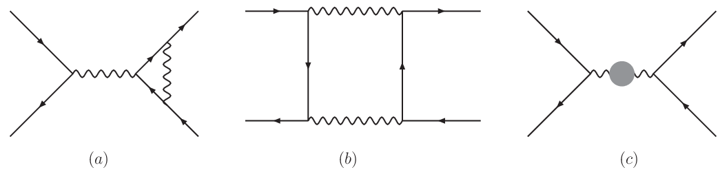
For the fermionic and hadronic corrections to Bhabha scattering at one-loop accuracy, there is only the self-energy diagram shown in Fig. 3(c). The two-loop irreducible self-energy contributions have the topology shown in Fig. 3(c). One has additionally the four classes of two-loop diagrams shown in Fig. 4 The reducible self-energy (Figure 4(a)) and vertex (Figure 4(b)) topologies are much easier to evaluate than the irreducible vertex (Figure 4(c)) and box (Figure 4(d)) topologies. In fact, only the two-loop boxes were unknown until quite recently.

The two-loop corrections have to be added with the loop-by-loop contributions (the interferences of the topologies of Fig. 3) and with the soft photon corrections. All these terms will be discussed in the following sections.

To summarize this section, the hadronic and heavy-fermion corrections to the Bhabha-scattering cross section can be obtained by replacing appropriately the photon propagator by a massive propagator, whose effective mass $z$ is subsequently integrated over. Inserting  (22) and  (27) in  (21) we get:

In the following, we will call the massive propagator function in (29) the self-energy kernel function:

The weight function $R(z)$ is given by the sum of the non-perturbative light-quark component of Eq. (28) and the perturbative result of Eq. (23), valid for leptons, $f=e,\mu,\tau$, and the top quark, $f=t$:

Compared to (23), we omit here the terms of order $O(\epsilon)$. The function $R_{\rm had}^{(5)}(z)$ will be discussed in Appendix E.

Corrections related to electron insertions ($f=e$) will be discussed separately. For pure self-energy insertions (see Appendix A), we may consider the electron mass as being small and neglect terms of order $O(m_{e}^{2}/x)$, $x=s,|t|,|u|$. At the expense of that, even the three-loop corrections are known [123]. For two-loop irreducible vertex and box corrections, we may either consider $m_{e}$ being finite and treat a two-scale problem ($s/m_{e}^{2},t/m_{e}^{2}$), or we may assume also here $m_{e}^{2}<<s,|t|,|u|$. Instead, for the diagrams with self-energy insertions of other fermions $f$, we will assume $m_{e}^{2}<<m_{f}^{2},s,|t|,|u|$, but we will make no additional assumption on $m_{f}^{2}$.

The pure vacuum polarization contributions to Bhabha scattering form a gauge invariant subset of diagrams. So, their numerics may be discussed separately. They can be readily obtained from the tree-level result  (2) by introducing appropriately a running fine-structure constant $\alpha(x)$, where $x=s,t$,

and where the running of $\alpha$ is defined as

Here $\Delta\alpha$ is given by the sum of the non-perturbative light-quark contribution $\Delta\alpha_{\rm had}^{(5)}$ [124] (see Refs. [125, 126, 127] and references therein for recent developments), a perturbative electron-loop component evaluated in the small electron-mass limit, $\Pi_{e}$, and a fermion-loop term computed exactly, $\Pi_{f}$, with $f=\mu,\tau,t$,

with the self-energy kernel function $K_{\rm SE}(x;z)$ (30).

For $x<4m_{\pi}^{2}$, Eq. (36) is well defined. For $x>4m_{\pi}^{2}$, the real and imaginary parts are after a subtraction:

The $\text{Im}\left[\Delta\alpha_{\rm had}^{(5)}(x)\right]$ coincides with Eq. (27). Expressions for the perturbative contributions to the photon vacuum-polarization function, $\Pi_{f}$ and $\Pi_{e}$, are available in QED exactly up to two loops [128] and in the small electron-mass limit up to three loops [123]. For convenience, their explicit expressions are collected in Appendix A. For our analysis, we use the exact results of Eqs. (A) and (A) for fermion loops ($f\neq e$), and the high-energy expressions of Eqs. (106), (107) and (107) for electron loops.

In Tables 1 and  2 we show numerical values for the various components of $\Delta\alpha$ of Eq. (35) for space-like and time-like values of $x$ ($t$- and $s$-channel). Note that $\Delta\alpha$ develops an imaginary part in the $s$-channel above the two-particle production threshold (see Table 1). Besides the Fortran package hadr5.f for hadronic contributions [129], we employed the Mathematica package HPL [130, 131] and, as a cross check, our Fortran routines (see Appendices A and F).

Hadronic and heavy-fermion irreducible vertex corrections are obtained through the interference of the diagrams of Figure 5 with the tree-level amplitude. The contributions from the irreducible vertices are gauge invariant by themselves. Their contribution to the ${\cal O}(\alpha^{2})$ differential cross section is given by

Here $V_{2}$ summarizes all two-loop fermionic corrections to the QED Dirac form factor, whose computation can be traced back to the seminal work of Refs. [133] and [134]. The full result can be organized as

where $V_{2e}$ denotes the electron-loop component. Closed analytical expressions in the case of electron loops at finite $m_{e}$ can be found in Ref. [95]. In the high-energy limit, compact expressions are available thanks to Ref. [135]:

After a combination with soft real electron pair emission contributions (150), the leading logarithmic contributions $\ln^{3}(s/m_{e}^{2})$ get cancelled in (39).

Heavy-fermion and hadronic contributions, instead, can be evaluated as in Ref. [121] through the dispersion integral

where $R$ is given in Eq. (31) and the two-loop irreducible vertex kernel function $K_{V}$, in the limit of a vanishing electron mass, reads as

Here $\text{Li}_{2}(x)$ is the usual dilogarithm and $\zeta_{2}={\rm{Li_{2}}}(1)=\pi^{2}/\penalty 6$. The kernel is at the upper integration boundary of the order $O(1/z)$, the integrand of order $O(1/z^{2})$ so that the dispersion integral is finite there:

At the lower integration bound, the integrand becomes for small $z/x$:

This asymptotic behavior yields at most terms of the order of $\ln^{3}(x/M^{2})$ if $M^{2}<<x$.

An interesting question is the identification of mass logarithms in case of fermion insertions. Let us rewrite:

where $V_{2{\rm had}}^{(5)}$ denotes the non-perturbative light-quark term and $V_{2f}$ the perturbative contribution of a fermion of flavor $f\neq e$. Potentially large logarithms arise from parts of the integrand for the $z$ integration which are singular at the lower integration bound, $z\to 4M^{2}$, when allowing thereby $M^{2}$ to become small. For fermions, one has to analyze $R_{f}(z)K_{V}(x;z)/z$ in that limit.

The corresponding analytical integrations may be performed easily after applying the transformation

thereby getting rid of the square root function in $R_{f}(z)$:

After that transformation, the dispersion integral becomes:

From the vertex kernel function $K_{V}(x;z)$, we have additionally dependences on $\ln(-x/z)$ and on ${\rm{Li_{2}}}(1+x/z)$. Although after the variable change (47) the arguments of logarithm and dilogarithm become non-linear, all the integrals may be taken trivially, and we will not go into further details. The result contains ${\rm{Li_{3}}}$ and powers of logarithms $\ln^{n}(x/m_{f}^{2})$ with $n\leq 3$. In fact, one will rediscover in the kinematically interesting ultra-relativistic case the formula known from  [135] and e.g. also from  [111]:

The same soft- real pair cancellation mechanism as described for electrons works also for heavy fermions, and the leading logarithmic powers $\ln^{3}(s/m_{f}^{2})$ will get cancelled in the cross-section. This is of physical relevance if the soft pair emissions remain unobserved. In our numerical studies, we will, conventionally, include the soft electron pair emission cross-section, but not that for heavy fermions or hadrons. For further details see Section D, and some numerical results were presented in [136], where we used the parameterization [132] with flag setting $\texttt{IPAR}=1$.

We just mention that the transformation (47), when applied to the simple one-loop self-energy kernel (30),

gives a rational integrand for the $u$-integration, and one gets as a result a function at most linear in $\ln(s/m_{f}^{2})$. For the explicit expressions see Equations (A) (constant term in $\epsilon$) and (106).

There are various origins of heavy-fermion or hadronic infrared divergent cross-section contributions of order $O(\alpha^{4})$:

• •

  Factorisable diagrams with one-loop vertex or box insertions

• •

  Irreducible two-loop box diagrams

• •

  soft real photon corrections

The sum of these corrections is gauge-invariant and infrared finite.

We will consider five classes of contributions:

• (a)

  Interference of Born diagrams with reducible [vertex+self-energy] corrections of Fig. 6;

• (b)

  Interference of one-loop vertex and self-energy diagrams, both of Fig. 3;

• (c)

  Interference of one-loop box and self-energy diagrams, both of Fig. 3;

• (d)

  Interference of real soft photon emission diagrams, one of them with a self-energy insertion;

• (box)

  Interference of Born diagrams with two-loop box diagrams of Figure 7.

For ease of notation, in the following we collect the overall dependence on $\alpha$ and rewrite the factorizing contributions of class $i$, $i=a,\ldots,d$:

and analogously for the two-loop boxes. In addition, we define

and introduce short-hand notations for those kinematic factors which appear more than once in the following formulas:

References

• [1] S. Actis et al., Phys. Rev. Lett. 100 (2008) 131602, 0711.3847.
• [2] H. Bhabha, Proc. Roy. Soc. A154 (1936) 195.
• [3] M. Consoli, Nucl. Phys. B160 (1979) 208.
• [4] M. Consoli, M. Greco and S. Lo Presti, Phys. Lett. B113 (1982) 415.
• [5] M. Caffo, R. Gatto and E. Remiddi, Nucl. Phys. B252 (1985) 378.
• [6] M. Böhm et al., Phys. Lett. B144 (1984) 414.
• [7] K. Tobimatsu and Y. Shimizu, Prog. Theor. Phys. 75 (1986) 905.
• [8] K. Tobimatsu and Y. Shimizu, Prog. Theor. Phys. 74 (1985) 567.
• [9] M. Böhm, A. Denner and W. Hollik, Nucl. Phys. B304 (1988) 687.
• [10] F. Berends, R. Kleiss and W. Hollik, Nucl. Phys. B304 (1988) 712.
• [11] D. Bardin, W. Hollik and T. Riemann, Z. Phys. C49 (1991) 485.
• [12] M. Awramik et al., Phys. Rev. D69 (2004) 053006, hep-ph/0311148.
• [13] M. Awramik, M. Czakon and A. Freitas, JHEP 11 (2006) 048, hep-ph/0608099.
• [14] F. Berends and G. Komen, Phys. Lett. B63 (1976) 432.
• [15] F. Berends and R. Kleiss, Nucl. Phys. B228 (1983) 537.
• [16] F.A. Berends, P.H. Daverveldt and R. Kleiss, Nucl. Phys. B253 (1985) 421.
• [17] M. Greco, Phys. Lett. B177 (1986) 97.
• [18] S. Kuroda et al., Comput. Phys. Commun. 48 (1988) 335.
• [19] D. Karlen, Nucl. Phys. B289 (1987) 23.
• [20] F. Aversa et al., Phys. Lett. B247 (1990) 93.
• [21] J. Fujimoto et al., Prog. Theor. Phys. Suppl. 100 (1990) 1.
• [22] M. Caffo, H. Czyz and E. Remiddi, Nuovo Cim. A105 (1992) 277.
• [23] M. Cacciari et al., Phys. Lett. B268 (1991) 441.
• [24] M. Cacciari et al., Phys. Lett. B271 (1991) 431.
• [25] W. Beenakker, F.A. Berends and S.C. van der Marck, Nucl. Phys. B349 (1991) 323.
• [26] W. Beenakker, F.A. Berends and S.C. van der Marck, Nucl. Phys. B355 (1991) 281.
• [27] F. Aversa and M. Greco, Phys. Lett. B271 (1991) 435.
• [28] S. Riemann, A Comparison of programs used in L3 for the analysis of Bhabha scattering, 1991, PHE-91-04.
• [29] V.S. Fadin et al., Small angles Bhabha scattering: Two loop approximation, 1992, JINR-E2-92-577.
• [30] K.S. Bjoerkevoll, P. Osland and G. Faeldt, Nucl. Phys. B386 (1992) 280.
• [31] K.S. Bjoerkevoll, P. Osland and G. Faeldt, Nucl. Phys. B386 (1992) 303.
• [32] D.Y. Bardin et al., ZFITTER: An analytical program for fermion pair production in e+​e−e^{+}e^{-} annihilation, 1992, hep-ph/9412201.
• [33] G. Montagna et al., Nucl. Phys. B401 (1993) 3.
• [34] M. Caffo, E. Remiddi and H. Czyz, Int. J. Mod. Phys. C4 (1993) 591.
• [35] J. Fujimoto, Y. Shimizu and T. Munehisa, Prog. Theor. Phys. 91 (1994) 333, hep-ph/9311368.
• [36] M. Caffo, H. Czyz and E. Remiddi, Phys. Lett. B327 (1994) 369.
• [37] M. Caffo, E. Remiddi and H. Czyz, The theoretical precision in small angle Bhabha scattering at LEP: Comparisons between different approaches, CERN 95-03 (1994) 361-368.
• [38] V.S. Fadin et al., Small angle Bhabha scattering with a 0.1% accuracy, Proc. 29th Rencontres de Moriond, 1994, p. 161.
• [39] A. Arbuzov et al., Small angle Bhabha scattering for LEP, 1995, hep-ph/9506323.
• [40] M. Cacciari et al., Comput. Phys. Commun. 90 (1995) 301, hep-ph/9507245.
• [41] J.H. Field and T. Riemann, Comput. Phys. Commun. 94 (1996) 53, hep-ph/9507401.
• [42] S. Jadach, W. Placzek and B.F.L. Ward, Phys. Lett. B390 (1997) 298, hep-ph/9608412.
• [43] A. Arbuzov et al., Nucl. Phys. B485 (1997) 457, hep-ph/9512344.
• [44] A.B. Arbuzov et al., Nucl. Phys. B474 (1996) 271.
• [45] A.B. Arbuzov et al., Phys. Atom. Nucl. 60 (1997) 591.
• [46] M. Caffo, H. Czyz and E. Remiddi, Phys. Lett. B378 (1996) 357, hep-ph/9603300.
• [47] M. Caffo and H. Czyz, Comput. Phys. Commun. 100 (1997) 99, hep-ph/9607357.
• [48] A. Arbuzov et al., Nucl. Phys. Proc. Suppl. 51C (1996) 154, hep-ph/9607228.
• [49] A. Arbuzov et al., Phys. Lett. B394 (1997) 218, hep-ph/9606425.
• [50] A.B. Arbuzov et al., Nucl. Phys. B483 (1997) 83, hep-ph/9610228.
• [51] A.B. Arbuzov et al., Phys. Lett. B399 (1997) 312, hep-ph/9612201.
• [52] S. Jadach et al., Nucl. Phys. Proc. Suppl. 51C (1996) 164, hep-ph/9607358.
• [53] S. Jadach et al., Comput. Phys. Commun. 102 (1997) 229.
• [54] S. Jadach et al., Event generators for Bhabha scattering, 1996, hep-ph/9602393.
• [55] S. Jadach et al., Phys. Lett. B377 (1996) 168, hep-ph/9603248.
• [56] W. Beenakker and G. Passarino, Phys. Lett. B425 (1998) 199, hep-ph/9710376.
• [57] M. Caffo, H. Czyz and E. Remiddi, Nuovo Cim. A110 (1997) 515, hep-ph/9704443.
• [58] A. Arbuzov et al., JHEP 10 (1997) 001, hep-ph/9702262.
• [59] N.P. Merenkov et al., Acta Phys. Polon. B28 (1997) 491.
• [60] A. Arbuzov, E. Kuraev and B. Shaikhatdenov, Mod. Phys. Lett. A13 (1998) 2305, hep-ph/9806215.
• [61] G. Montagna et al., Nucl. Phys. B547 (1999) 39, hep-ph/9811436.
• [62] A.B. Arbuzov, E.A. Kuraev and B.G. Shaikhatdenov, J. Exp. Theor. Phys. 88 (1999) 213, hep-ph/9805308, E: JETP 97 (2003) 858.
• [63] D. Bardin et al., Comput. Phys. Commun. 133 (2001) 229, hep-ph/9908433.
• [64] A. Arbuzov, LABSMC: Monte Carlo event generator for large-angle Bhabha scattering, 1999, hep-ph/9907298.
• [65] W. Placzek et al., Precision calculation of Bhabha scattering at LEP, 1999, hep-ph/9903381.
• [66] S. Jadach, B.F.L. Ward and Z. Was, Comput. Phys. Commun. 124 (2000) 233, hep-ph/9905205.
• [67] G. Montagna, O. Nicrosini and F. Piccinini, Phys. Lett. B460 (1999) 425, hep-ph/9904387.
• [68] C.M. Carloni Calame et al., Large-angle Bhabha scattering and luminosity at DAPHNE, 1999, hep-ph/0001131.
• [69] V. Antonelli, E.A. Kuraev and B.G. Shaikhatdenov, Nucl. Phys. B568 (2000) 40, hep-ph/9905331.
• [70] C.C. Calame et al., Nucl. Phys. B584 (2000) 459, hep-ph/0003268.
• [71] M. Battaglia, S. Jadach and D. Bardin, eConf C010630 (2001) E3015.
• [72] C.M. Carloni Calame, Phys. Lett. B520 (2001) 16, hep-ph/0103117.
• [73] D. Karlen and H. Burkhardt, Eur. Phys. J. C22 (2001) 39, hep-ex/0105065.
• [74] B.F.L. Ward, S. Jadach and Z. Was, Nucl. Phys. Proc. Suppl. 116 (2003) 73, hep-ph/0211132.
• [75] S. Jadach, Theoretical error of luminosity cross section at LEP, 2003, hep-ph/0306083.
• [76] A. Arbuzov et al., Eur. Phys. J. C34 (2004) 267, hep-ph/0402211.
• [77] J. Fleischer, A. Lorca and T. Riemann, Automatized calculation of 2-fermion production with DIANA and aiTALC, in Proc. LCWS, Paris, 2004, hep-ph/0409034.
• [78] J. Gluza, A. Lorca and T. Riemann, Nucl. Instrum. Meth. 534 (2004) 289, hep-ph/0409011.
• [79] A. Lorca and T. Riemann, Nucl. Phys. Proc. Suppl. 135 (2004) 328, hep-ph/0407149.
• [80] A.B. Arbuzov et al., Eur. Phys. J. C46 (2006) 689, hep-ph/0504233.
• [81] A. Arbuzov et al., Comput. Phys. Commun. 174 (2006) 728, hep-ph/0507146.
• [82] A.B. Arbuzov and E.S. Scherbakova, JETP Lett. 83 (2006) 427, hep-ph/0602119.
• [83] G. Balossini et al., Nucl. Phys. Proc. Suppl. 162 (2006) 59, hep-ph/0610022.
• [84] G. Balossini et al., Nucl. Phys. B758 (2006) 227, hep-ph/0607181.
• [85] J. Fleischer et al., Eur. J. Phys. 48 (2006) 35, hep-ph/0606210.
• [86] K. Mönig, Bhabha scattering at the ILC, talk at Bhabha Workshop, Karlsruhe, April 2005, http://sfb-tr9.particle.uni-karlsruhe.de/.
• [87] A. Denig, Bhabha scattering at Dafne: The Kloe luminosity measurement, talk at Bhabha Workshop of SFB/TRR 9, Karlsruhe, April 2005, http://sfb-tr9.particle.uni-karlsruhe.de/veranstaltungen/bhabha-talks/denig.pdf.
• [88] L. Trentadue, Measurement of αQ​E​D\alpha_{QED}: An alternative approach, talk at Bhabha Workshop of SFB/TRR 9, Karlsruhe, April 2005, http://sfb-tr9.particle.uni-karlsruhe.de/veranstaltungen/bhabha-talks/trentadue.pdf.
• [89] S. Jadach, Theoretical calculations for LEP luminosity measurements, talk at Bhabha Workshop of SFB/TRR 9, Karlsruhe, April 2005, http://sfb-tr9.particle.uni-karlsruhe.de/veranstaltungen/bhabha-talks/jadach.pdf.
• [90] G. Balossini et al., Acta Phys. Polon. B38 (2007) 3441.
• [91] G. Balossini et al., Mini-review on Monte Carlo programs for Bhabha scattering, to appear in Proc. Loops and Legs, Sondershausen, 2008, arXiv:0806.4909 [hep-ph].
• [92] V. Smirnov, Phys. Lett. B524 (2002) 129, hep-ph/0111160.
• [93] Z. Bern, L. Dixon and A. Ghinculov, Phys. Rev. D63 (2001) 053007, hep-ph/0010075.
• [94] N. Glover, B. Tausk and J. van der Bij, Phys. Lett. B516 (2001) 33, hep-ph/0106052.
• [95] R. Bonciani, P. Mastrolia and E. Remiddi, Nucl. Phys. B676 (2004) 399, hep-ph/0307295.
• [96] R. Bonciani et al., Nucl. Phys. B681 (2004) 261, hep-ph/0310333.
• [97] R. Bonciani, P. Mastrolia and E. Remiddi, Nucl. Phys. B661 (2003) 289, hep-ph/0301170.
• [98] R. Bonciani et al., Nucl. Phys. B716 (2005) 280, hep-ph/0411321v2.
• [99] M. Czakon, J. Gluza and T. Riemann, Nucl. Phys. Proc. Suppl. 135 (2004) 83, hep-ph/0406203.
• [100] M. Czakon, J. Gluza and T. Riemann, Phys. Rev. D71 (2005) 073009, hep-ph/0412164.
• [101] G. Heinrich and V. Smirnov, Phys. Lett. B598 (2004) 55, hep-ph/0406053.
• [102] A. Penin, Phys. Rev. Lett. 95 (2005) 010408, hep-ph/0501120.
• [103] A. Penin, Nucl. Phys. B734 (2006) 185, hep-ph/0508127.
• [104] R. Bonciani and A. Ferroglia, Phys. Rev. D72 (2005) 056004, hep-ph/0507047.
• [105] M. Czakon, J. Gluza and T. Riemann, Acta Phys. Polon. B36 (2005) 3319, hep-ph/0511187.
• [106] R. Bonciani and A. Ferroglia, Nucl. Phys. Proc. Suppl. 157 (2006) 11, hep-ph/0601246.
• [107] M. Czakon, J. Gluza and T. Riemann, Nucl. Phys. B751 (2006) 1, hep-ph/0604101.
• [108] A. Mitov and S. Moch, JHEP 05 (2007) 001, hep-ph/0612149.
• [109] S. Actis, M. Czakon, J. Gluza, T. Riemann, Nucl. Phys. Proc. Suppl. 160 (2006) 91, hep-ph/0609051.
• [110] T. Becher and K. Melnikov, JHEP 06 (2007) 084, arXiv:0704.3582 [hep-ph].
• [111] S. Actis et al., Nucl. Phys. B786 (2007) 26, arXiv:0704.2400v.2 [hep-ph].
• [112] S. Actis et al., Acta Phys. Polon. B38 (2007) 3517, 0710.5111.
• [113] S. Actis et al., Fermionic NNLO contributions to Bhabha scattering, XXXI Conference “Matter to the Deepest”, Ustroń, Poland, 5-11 Sep 2007, http://prac.us.edu.pl/∼\simus2007/talks.htm.
• [114] R. Bonciani, A. Ferroglia and A.A. Penin, Phys. Rev. Lett. 100 (2008) 131601, 0710.4775.
• [115] J. Fleischer et al., Acta Phys. Polon. B38 (2007) 3529, arXiv:0710.5100 [hep-ph].
• [116] R. Bonciani, A. Ferroglia and A.A. Penin, JHEP 02 (2008) 080, 0802.2215.
• [117] DESY, webpage http://www-zeuthen.desy.de/theory/research/bhabha/bhabha.html.
• [118] W.-M. Yao et al. [the Particle Data Group], J. Phys. G 33 (2006) 1.
• [119] N. Cabibbo and R. Gatto, Phys. Rev. 124 (1961) 1577.
• [120] R.E. Cutkosky, J. Math. Phys. 1 (1960) 429.
• [121] B. Kniehl et al., Phys. Lett. B209 (1988) 337.
• [122] T. van Ritbergen and R.G. Stuart, Phys. Lett. B437 (1998) 201, hep-ph/9802341.
• [123] M. Steinhauser, Phys. Lett. B429 (1998) 158, hep-ph/9803313.
• [124] S. Eidelman and F. Jegerlehner, Z. Phys. C67 (1995) 585, hep-ph/9502298.
• [125] H. Burkhardt and B. Pietrzyk, Phys. Rev. D72 (2005) 057501, hep-ph/0506323.
• [126] F. Jegerlehner, Nucl. Phys. Proc. Suppl. 162 (2006) 22, hep-ph/0608329.
• [127] K. Hagiwara et al., Phys. Lett. B649 (2007) 173, hep-ph/0611102.
• [128] G. Kallen and A. Sabry, Kong. Dan. Vid. Sel. Mat. Fys. Med. 29N17 (1955) 1.
• [129] F. Jegerlehner, Fortran program hadr5.f (version 02 Nov 2003), available at http://www-com.physik.hu-berlin.de/ fjeger.
• [130] D. Maitre, Comput. Phys. Commun. 174 (2006) 222, hep-ph/0507152.
• [131] D. Maitre, Extension of HPL to complex arguments, 2007, hep-ph/0703052.
• [132] H. Burkhardt, New numerical analysis of the hadronic vacuum polarization, TASSO-NOTE-192 (1981), and Fortran program repi.f (1986).
• [133] R. Barbieri, J.A. Mignaco and E. Remiddi, Nuovo Cim. A11 (1972) 824.
• [134] R. Barbieri, J.A. Mignaco and E. Remiddi, Nuovo Cim. A11 (1972) 865.
• [135] G. Burgers, Phys. Lett. B164 (1985) 167.
• [136] S. Actis, J. Gluza and T. Riemann, Virtual Hadronic Corrections to Massive Bhabha Scattering, 2008, 0807.0174, contrib. to Loops and Legs 2008, to appear in Nucl. Phys. B (PS).
• [137] J. Gluza, K. Kajda and T. Riemann, Comput. Phys. Commun. 177 (2007) 879, arXiv:0704.2423 [hep-ph].
• [138] M. Czakon, Comput. Phys. Commun. 175 (2006) 559, hep-ph/0511200.
• [139] J. Frenkel and J.C. Taylor, Nucl. Phys. B116 (1976) 185.
• [140] J.H. Kuhn and S. Uccirati, (2008), 0807.1284.
• [141] S. Actis, M. Czakon, J. Gluza and T. Riemann,
http://www-zeuthen.desy.de/theory/research/bhabha/bhabha.html/.
• [142] M. Melles, Acta Phys. Polon. B28 (1997) 1159, hep-ph/9612348.
• [143] S. Jadach, B.F.L. Ward and Z. Was, Comput. Phys. Commun. 130 (2000) 260, hep-ph/9912214.
• [144] Two Fermion Working Group, M. Kobel et al., Two-fermion production in electron positron collisions, 2000, hep-ph/0007180.
• [145] R. Bonciani et al., Nucl. Phys. B701 (2004) 121, hep-ph/0405275.
• [146] J. Fleischer et al., Eur. Phys. J. C31 (2003) 37, hep-ph/0302259.
• [147] M. Davier et al., Eur. Phys. J. C27 (2003) 497, hep-ph/0208177.
• [148] NA7, S.R. Amendolia et al., Nucl. Phys. B277 (1986) 168.
• [149] Fortran routine, private communications with T. Teubner. The Fortran program is based on the data compilation performed for [154, 127]. The publication is in preparation. The routine is available upon request from the authors, E-mails: dnomura@post.kek.jp, thomas.teubner@liverpool.ac.uk. We used version of 2008-04-26.
• [150] R.V. Harlander and M. Steinhauser, Comput. Phys. Commun. 153 (2003) 244, hep-ph/0212294.
• [151] G. ’t Hooft and M. Veltman, Nucl. Phys. B153 (1979) 365.
• [152] J. Vollinga and S. Weinzierl, Comput. Phys. Commun. 167 (2005) 177, hep-ph/0410259.
• [153] R. Crandall, Note on fast polylogarithm computation, 2006, http://people.reed.edu/∼\simcrandall/papers/Polylog.pdf.
• [154] K. Hagiwara et al., Phys. Rev. D69 (2004) 093003, hep-ph/0312250.
• [155] J.A.M. Vermaseren, Comput. Phys. Commun. 83 (1994) 45.
• [156] D. Binosi and L. Theussl, Comput. Phys. Commun. 161 (2004) 76, hep-ph/0309015.