Estimating Jones and HOMFLY polynomials with One Clean Qubit
Abstract
The Jones and HOMFLY polynomials are link invariants with close connections to quantum computing. It was recently shown that finding a certain approximation to the Jones polynomial of the trace closure of a braid at the fifth root of unity is a complete problem for the one clean qubit complexity class[18]. This is the class of problems solvable in polynomial time on a quantum computer acting on an initial state in which one qubit is pure and the rest are maximally mixed. Here we generalize this result by showing that one clean qubit computers can efficiently approximate the Jones and single-variable HOMFLY polynomials of the trace closure of a braid at any root of unity.
1 Introduction
A knot is an embedding of the circle into three dimensional space. More generally, a link is an embedding of one or more circles into three dimensional space. A link is said to be oriented if one of the two possible orientations is chosen for each circle. Examples are shown in figure 1.
Two links are equivalent if one can be continuously deformed into the other without cutting any strands. One of the most fundamental tasks in the theory of links is to determine whether a given pair of links is equivalent. Although this task appears easy in the simple examples of figure 1, it rapidly becomes difficult for links of many crossings. No polynomial time algorithm for this problem is known. Currently the best upper bound on the complexity of the link equivalence problem is that it is contained in NP [10].
Link invariants are one tool for distinguishing links. A link invariant is some function on links such that if link is equivalent to link then . There may exist inequivalent links that a given link invariant fails to distinguish. The Jones polynomial is an important link invariant that has been very successful in distinguishing inequivalent links. It was discovered in 1985 by Vaughan Jones [12]. For an oriented link with crossings, the corresponding Jones polynomial is a polynomial consisting of a linear combination of integer and half-integer powers of . has degree at most , and the coefficients in the polynomial are all integers. That is, . The coefficients may be exponentially large, and finding their values exactly is known to be #P-complete[11].

In order to formulate computational problems about links, one needs a way to input links into a computer. One way to do this is to use the discrete language of the braid group. A braid of strands has pegs across the top and pegs across the bottom. Each top peg is the starting point of exactly one strand. Each bottom peg is the end point of exactly one strand. On the way, the strands can wind around each other in any arbitrary way, but cannot “double back,” as illustrated in figure 2. Two braids are equivalent if one can be deformed into the other without cutting any strands.

The set of braids on strands has the structure of a group. The
group operation is concatenation of braids, as shown below.
![[Uncaptioned image]](0807.4688v2/concatenation.png)
The -strand braid group is generated by the elementary
crossings as illustrated below.
![[Uncaptioned image]](0807.4688v2/generators_spj.png)
For example, the braid of figure 2 is . The topological equivalence of braids is completely captured by the following two relations among the group generators.
| (1) |
By joining the free ends of a braid, one can construct a link. Figure 3 illustrates two ways of doing this: the plat closure and the trace closure. Alexander’s theorem states that any link can be obtained as the trace closure of some braid. The same is true of the plat closure[18].

In addition to gaining a convenient way for inputting links into computers, by thinking of links in terms of the braid group, we gain an algebraic point of view on the topological problem of distinguishing links. Jones originally formulated his polynomial in terms of certain representations of the braid group[12]. This original representation-theoretic formulation is also convenient for use in quantum computation. We’ll now describe it.
Let be a braid of strands and let be the
link obtained by taking its trace closure. If each strand of the braid
is oriented downward, then an oriented link results from
taking the trace closure. The Jones polynomial of at is
| (2) |
where is the “writhe” of . A crossing of
oriented strands of the form
![[Uncaptioned image]](0807.4688v2/poscross.png) is considered positive, and a crossing of the form
is considered positive, and a crossing of the form
![[Uncaptioned image]](0807.4688v2/negcross.png) is considered
negative. is equal to the number of positive
crossings minus the number of negative crossings in
. is the path model representation of the braid
group . is a certain weighted trace known as
the Markov trace. It is clear that the prefactor
is easy to calculate, thus the problem of evaluating
Jones polynomials polynomial-time reduces to the evaluation of the
Markov trace of the path model representation.
is considered
negative. is equal to the number of positive
crossings minus the number of negative crossings in
. is the path model representation of the braid
group . is a certain weighted trace known as
the Markov trace. It is clear that the prefactor
is easy to calculate, thus the problem of evaluating
Jones polynomials polynomial-time reduces to the evaluation of the
Markov trace of the path model representation.
In 1989, Witten proved that the Jones polynomial arises as a Wilson loop in Chern-Simons theory, thereby uncovering a connection between topological quantum field theory and knot invariants[19]. In 2002, Freedman et al. showed that quantum computers can efficiently simulate certain topological quantum field theories[8], and furthermore that the problem of simulating these topological quantum field theories is BQP-complete[9]. The results of Freedman et al. combined with that of Witten imply that quantum computers can efficiently estimate the Jones polynomial of the plat closure of a braid at and furthermore that this problem is BQP-complete. Aharonov et al. subsequently generalized this result, showing that quantum computers can efficiently estimate the Jones polynomial of the plat or trace closure of a braid at for any [3]. In [1, 7, 20, 9], the problem of estimating the Jones polynomial of the plat closure of a braid was shown to be BQP-complete for each other than 1,2,3,4, and 6. The problem of estimating the Jones polynomial of the trace closure of a braid at was shown in [18] to be complete for the one clean qubit complexity class, called DQC1.
Whereas the Jones polynomial of the trace closure of a braid is proportional to the Markov trace of its path model representation, the Jones polynomial of the plat closure of a braid is proportional to a certain matrix element of its path model representation. For , the path model representation is unitary. The dimension of the representation is in general exponential in . Thus the direct classical algorithm for calculating the representation of a braid by multiplying the matrices representing individual crossings requires exponential time. In contrast, a quantum circuit on qubits corresponds to an element of . By the path model representation, a braid on strands corresponds to an exponentially large unitary matrix, which in turn corresponds to a quantum circuit on qubits. The nontrivial achievement of [8, 3, 20, 18] is to show that the number of gates in the quantum circuit need only grow polynomially with the number of crossings in the braid.
Such a correspondence between braids and quantum circuits forms the core of the completeness proofs for Jones polynomial problems. Estimating a matrix element of a quantum circuit to polynomial precision is BQP-complete, and estimating the normalized trace of a quantum circuit to polynomial precision is DQC1-complete. Constructing the correspondence between braids and circuits is slightly more involved in the case of DQC1-completeness essentially because the circuit can only use logarithmically many ancilla qubits[18].
The approximations to Jones polynomials obtained by quantum computers are additive. The Markov trace has magnitude at most one. The quantum algorithm for approximating the trace closure produces an estimate satisfying with probability in time. It is important to distinguish this from the other common type of approximation known as a Fully Polynomial Randomized Approxation Scheme (FPRAS). An FPRAS for a function produces an estimate satisfying with probability in time . For many braids , is exponentially small compared to one. For these instances, an FPRAS is exponentially more precise than a polynomial additive approximation.
The discovery of the Jones polynomial broke open a new field. A number of new and powerful knot invariants related to the Jones polynomial were soon discovered. The HOMFLY polynomial11 1 The name HOMFLY stands for the names of the discoverers of this invariant: Hoste, Ocneanu, Millett, Freyd, Lickorish, and Yetter. Some authors prefer the name HOMFLYPT polynomial to recognize the contributions of Przytycky and Traczyk. We will use the term HOMFLY polynomial simply because it is more widespread. is one of these. Like the Jones polynomial, the HOMFLY polynomial is an invariant of oriented links. In general the HOMFLY polynomial is a polynomial in two variables, . An important special case is the single-variable HOMFLY polynomial
also known as the invariant. As discussed in the appendix, the Jones polynomial is equivalent to the special case of the single-variable HOMFLY polynomial. In [20], Wocjan and Yard showed that quantum computers can efficiently approximate single-variable HOMFLY polynomials at arbitrary roots of unity. The HOMFLY polynomial is in turn a special case of an extremely general combinatorial object called the Tutte polynomial. Aharonov et al. have obtained efficient quantum algorithms for approximating Tutte polynomials[2]. It is not yet fully known for what range of parameters the approximation obtained in [2] is BQP-hard.
The one clean qubit model was introduced in [13] as an idealized model of quantum computation on highly mixed states. For example, the states manipulated in NMR experiments are typically highly mixed. One clean qubit computers are believed to be less powerful than standard quantum computers but still capable of solving some problems outside of P. In the one clean qubit model one is given an initial state consisting of one qubit in the pure state and qubits in the maximally mixed state. In other words, the initial density matrix is
where is the identity matrix. One is then allowed to apply polynomially many quantum gates to this state, and then do a single-qubit measurement in the computational basis. This procedure can be repeated polynomially many times, each time starting with the same initial state . The set of decision problems solvable by this procedure is called DQC1.
Here we show that one clean qubit computers can efficiently estimate Jones and HOMFLY polynomials at arbitrary roots of unity, generalizing the result of [18]. To do this we need only two facts about one clean qubit computers. First, one clean qubit computers can efficiently estimate the normalized trace of quantum circuits to polynomial precision22 2 Although we do not need this fact here, it is interesting to note that the decision version of this problem is DQC1-complete.. That is, we are given a classical description of a quantum circuit on qubits with gates. This quantum circuit implements some unitary transformation on a -dimensional Hilbert space. The quantity is a complex number of magnitude at most one. One clean qubit computers can produce an estimate of such that with probability , in time . Second, a computer with one clean qubit can simulate a computer with clean qubits with polynomial overhead. Both of these facts are discussed thoroughly in [18]. For additional information about one clean qubit computers we refer the interested reader to [13, 14, 16, 17, 4, 18, 6].
2 Path Model Representation of
As discussed in section 1 and reference [3], the problem of estimating the Jones polynomial of the trace closure of a braid reduces to the problem of estimating the Markov trace of the braid’s path model representation. In this section we present the path model representation of the braid group , and the Markov trace of this representation.
Let be the set of paths of steps on a ladder of rungs that start at the bottom. For example
Let be the formal span of and let be its dual. For example
where for any :
For any the path model representation is a homomorphism from , the -strand braid group, to , the group of unitary transformations on .
Let denote the crossing of strands and :
![[Uncaptioned image]](0807.4688v2/crossing.png) |
acts only on steps and of paths in leaving the other steps unchanged. Specifically,
![[Uncaptioned image]](0807.4688v2/crossrep2.png) |
And similarly,
where:
These rules completely define the representation .
Let be the set of paths in that end on rung . Let be the corresponding -dimensional vector space. leaves unchanged for all , as one can see from the preceding rules. Thus, for each , these rules define a representation . is the direct sum of these.
The Markov trace of the representation is given by:
| (3) |
where is the ordinary matrix trace, and .
In section 4 we show how to estimate the normalized trace
| (4) |
on a one clean qubit computer for each . Given the ability to do this, it is a simple matter to obtain the full Markov trace. By equation 3 we see that we can obtain the Markov trace by classically sampling according to the distribution
For each obtained by sampling from this distribution, we use a one clean qubit computer to estimate the corresponding normalized trace of equation 4. By construction, the average obtained by this sampling procedure will converge to the Markov trace. By taking polynomially many samples, one can obtain the Markov trace to polynomial precision. The probability distribution is easy to sample from because can take on only different values, and each is furthermore easy to compute.
To estimate the normalized trace (eq. 4) on a one clean qubit computer, we introduce an encoding from bits to paths
where is a parameter whose value we determine in section 3. is a non-injective map. However, the number of different bitstrings that map to a given path is approximately the same for all paths. That is, for all where is the number of bitstrings in that get mapped to .
For any with crossings we obtain a quantum circuit of gates such that for almost all ,
| (5) |
In other words, this quantum circuit implements the path model representation of braid . Thus
With such an encoding we are able to use maximally mixed qubits to obtain a uniformly weighted trace over all paths in .
3 Encoding Paths as Bitstrings
To describe we imagine a randomized classical algorithm which uses random bits to produce an element of approximately uniformly at random. Such an algorithm corresponds to a map from to , and the fact that the probability distribution over paths is approximately uniform ensures that
for all . This algorithm is not to be run, but is rather a conceptual tool for the design of the encoding .
The algorithm works by starting at the bottom rung, and adding steps one by one until a path of steps is obtained. Let be the number of paths of steps on a ladder of rungs which start at rung and end at rung . Suppose the current path has steps and ends at rung . There are completions of this path in which step is upward and completions in which step is downward. Thus the algorithm chooses step to be upward with probability
| (6) |
(To cover the cases and we define .) By choosing each step according to equation 6, one obtains at the end a uniform distribution over . This is illustrated in figure 4.

To generate a path of steps, we use registers of random bits. We think of the registers as encoding numbers in the range . The step is chosen to be up if and only if
| (7) |
Note that if the path has reached the top or bottom rung can equal 1 or 0.
If were implemented exactly then the paths would be produced with exactly uniform probability. Because of the rounding shown in equation 7, each is only accurate to within . Correspondingly, the number of bitstrings that get mapped by to a given path is not precisely the same for all paths. This introduces an error into the estimate of the normalized trace given by
By the definition of this is
where is the distribution over paths produced by the classical algorithm using bits of precision, and is the uniform distribution. By the triangle inequality,
Because is unitary this gives us
| (8) | |||||
Here we are thinking of probability distributions as vectors and measuring their distance using the 1-norm.
For the purpose of estimating Jones polynomials in DQC1, one wants to estimate the normalized trace to polynomial precision. Thus it suffices to have
| (9) |
As proven below, to satisfy the condition 9, it is sufficient to implement each to polynomial precision. Thus it is sufficient to choose .
Let
As shown in figure 4, our classical probabilistic algorithm can be thought of as a Markov process on . Each element in probabilistically transitions to one of two possible elements in with probabilities and . Hence we can define a -dimensional stochastic matrix representing our idealized algorithm. Each row contains at most two nonzero entries which are and . The initial probability distribution on has probability one on the zero step path:
After choosing steps, the probability distribution is
which has support only on paths of steps. We define analogously to , except that instead of and the entries represent the actual transition probabilities obtained using bits of precision. Thus, in each row, and have at most two nonzero entries (at the same places) and these entries differ by at most . Thus, in each row, has only two nonzero entries, each of magnitude bounded by . Hence for any probability distribution ,
| (10) | |||||
Let be the probability distribution obtained on -step paths by the actual algorithm and let be that obtained by the idealized algorithm. Further, let .
So:
and by the triangle inequality
is a stochastic matrix and therefore for any . Thus
by equation 10. Since , the final error is bounded by
is exactly the expression appearing in equation 8, thus choosing suffices to make polynomially small.
4 Algorithm for Jones Polynomials
With the encoding in place, the remaining task is to efficiently implement with a quantum circuit, as described in equation 5. To do this, it suffices to efficiently implement for each crossing . Then, to represent any -crossing braid we can concatenate the corresponding quantum circuits to obtain .
As discussed in section 2, transforms only steps and in any path. Hence transforms only registers and of qubits each in any encoded path. However, the transformation on these two steps depends on the rung on which they start. Each register encodes whether a given step is up or down. Thus, is encoded in the preceding registers. The number of rungs is fixed at , thus only a constant number of ancilla qubits () are needed to store . As discussed in section 1, up to logarithmically many clean ancilla qubits can be simulated on a one clean qubit computer. We will now describe how to efficiently compute into a register of clean ancilla qubits using reversible computation. (We assume is constant, unlike .)
To do this, we start by precomputing the cutoffs for all and on a standard classical computer. To store these numbers requires bits, which for any fixed is of order . By equation 6, we can compute these cutoffs by counting the number of paths of given length that begin and end on given rungs.
Let be the adjacency matrix of the line graph of nodes .
Then, the number of paths of length from rung to rung is the matrix element of . This can clearly be computed in time.
Suppose we have one register of qubits containing , the rung of step , and one register of qubits initialized to zero in which we wish to write . is simply set to or depending on whether the -qubit register in the encoding contains a number less or greater than the corresponding cutoff . Comparing two numbers to see which is bigger can be done reversibly using logarithmically many ancillas, and the same is true for adding or subtracting 1 to a number. (See section 4 of [18] for a summary of the literature on reversible arithmetic with limited ancillas.) Since the cutoffs are hardcoded they do not need to be computed reversibly at all. Thus this whole process is doable in DQC1. One then uncomputes and repeats this process until is obtained for the desired . Thus starting with , one can efficiently produce a register of qubits containing .
To implement we first compute and then use a unitary that acts on three registers: the and registers of qubits from the encoding and the register containing . does not affect the register. Rather, controls what operation gets applied to the other two registers, as specified by the path model representation. Thus, after applying , one can uncompute .
acts on qubits. By general techniques it is possible to implement arbitrary unitary transformations on qubits using gates[15]. Thus efficiency is not a concern. We just need to construct a concrete unitary implementation of that gives the correct transformation on the encoded paths as specified by the path model representation.
If the encoded path is
![[Uncaptioned image]](0807.4688v2/upordown.png) |
then, by the path model representation, we merely need to apply a phase shift of . If the encoded path is
![[Uncaptioned image]](0807.4688v2/bent.png) |
then we must unitarily transform to some linear combination of the encodings of these two paths.
There are possible values for the bits contained in the
relevant two registers. Suppose that the number of these bitstrings
that encode ![[Uncaptioned image]](0807.4688v2/udsmall.png) is equal to the
number of bitstrings that encode
is equal to the
number of bitstrings that encode
![[Uncaptioned image]](0807.4688v2/dusmall.png) . (As we shall see, these
two numbers are equal up to rounding.) Let’s call this number
. Then, we can use the labels:
. (As we shall see, these
two numbers are equal up to rounding.) Let’s call this number
. Then, we can use the labels:
for the bitstrings that encode
, and
for the bitstrings that encode
. Therefore, for each , is
| (11) |
in accordance with section 2. This is unitary and satisfies equation 5.
Looking in more detail at we can specify concretely the labelling. We can think of the contents of the and registers as specifying two numbers . Correspondingly we have the cutoffs
The bitstrings with , encode
, and the bitstrings with
, encode
. By the definition of
, the probability of hopping up and then down is
the same as the probability of hopping down and then up. This is
because both processes end on the same rung, thus each of these paths
have the same number of completions ending at height after
additional steps. Hence, up to rounding, the number of bitstrings from
the possibilities that encode
is the same as the
number of bitstrings that encode
. We can choose the label
from equation 11 to be:
| (12) |
Because of rounding to the nearest integer, is
only calculated to accuracy . Thus, the number of
bitstrings encoding can
exceed the number of bitstrings encoding
by as much as or vice versa. To achieve unitarity we define
to act as the identity on these excess bitstrings. We
therefore refer to these strings as “stuck”.
We will now show that, because these stuck bitstrings form at most a fraction of all the encodings on which acts, the error introduced by them is negligible, provided . We can divide the set of bitstrings into those that are stuck and those that are unstuck. By unitarity, no operator can ever transform an unstuck string into a stuck string or vice versa.
The total error introduced by the stuck strings is
For unstuck strings, , thus
where is the set of stuck strings. By the triangle inequality
By unitarity these matrix elements have at most unit magnitude, so
Thus is at most twice the fraction of strings in that are stuck. For each , the pair of registers and has probability approximately of being stuck. Thus the fraction of bitstrings in which at least one pair is stuck is approximately
By choosing we can thus ensure that is polynomially small.
The total error in the estimate of the normalized trace is
We can see this as follows.
(We have added and subtracted , leaving the total unchanged.) Applying the triangle inequality we obtain
The first term is recognizable as , and the second term is recognizable as , thus we are done.
5 HOMFLY polynomials
As discussed in section 1, the Jones polynomial is equivalent to a special case of a more general knot invariant called the single-variable HOMFLY polynomial. Let be the trace closure of a braid . To make an oriented link, every strand of the braid is oriented downward. The single-variable HOMFLY polynomial is
| (13) |
where is the Jones-Wenzl representation of , indicates its Markov trace (to be defined shortly), and is the sum of the exponents appearing in when written in terms of the generators . Thus, is minus the writhe of . For each and , the Jones-Wenzl representation is a unitary representation of the group , whose dimension is exponential in . In section 6, we will describe how to efficiently implement this unitary representation with quantum circuits, thereby allowing the efficient estimation of single-variable HOMFLY polynomials using one clean qubit. In the present section we will first describe the Jones-Wenzl representation and its Markov trace. Our presentation closely33 3 However, for consistency with [3, 18], we use and to represent the parameters called and , respectively, in [20]. follows that of [20].
The Jones-Wenzl representation of , the braid group of -strands, is formulated in terms of standard Young tableaux of boxes. For any , the Young diagrams are all the possible partitions of boxes into rows, where the rows are arranged in descending order of length. All the Young diagrams for are illustrated in figure 5. For a given Young diagram the corresponding standard Young tableaux are all the numberings of boxes so that if we started with no boxes, and added boxes in this order, the configuration would be a valid Young diagram after every step. An example is shown in figure 6.
For the reader intrigued by the appearance of Young tableaux we make the following aside. Young tableaux were originally introduced to construct representations of the symmetric group (cf. [5]). is closely related to ; the latter is obtained from the former by adding the relation . Any representation of the symmetric group must satisfy . By deforming this relation to we obtain the path model representation of . (The correspondence between paths and standard Young tableaux and the relationship between the path model and Jones-Wenzl representations are explained in the appendix.) This type of deformation appears frequently in mathematics and is referred to as a quantum deformation or -deformation. In the limit we recover a representation of . The origin of the term quantum deformation is the commutation relation among the position and momentum operators in quantum mechanics. This is a deformation of the classical commutation relation .
We now describe in detail the Jones-Wenzl representation of . Let be the set of standard Young tableaux of boxes and at most rows, such that after every step, the configuration is not only a valid Young diagram, but also has the property that the number of boxes in the first row minus the number of boxes in the row is at most . Let be the formal span of . For given , the Jones-Wenzl representation is a group homomorphism from the braid group to the group of unitary transformations on the vector space .


The elementary crossings generate the
braid group . Thus, to specify the representation
it suffices to specify the representations of these crossings
, as is done
by the following rule. For any :
| (14) |
where is the Young tableau obtained from by swapping boxes and , and is the “axial” distance from box to box in . That is, if box appears in row and column and box appears in row and column then
| (15) |
For some , the Young tableau obtained by swapping boxes and is not contained in . However, one can verify that in such cases, the coefficient is always zero. Thus, equation 14 defines a linear transformation strictly within .
By swapping boxes, one never changes the shape of a Young tableau. Thus, the Jones-Wenzl representation is reducible, with invariant subspaces corresponding to different Young diagrams. The Markov trace is the following weighted sum of the traces over these subspaces.
| (16) |
where is the Jones-Wenzl representation on the subspace corresponding to Young diagram , denotes the ordinary matrix trace, and the sum is over all Young diagrams of boxes and at most rows such that the number of boxes in the top row minus the number of boxes in the row is at most . The weights are given by
| (17) |
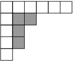
where the product is over all (row,column) coordinates in the Young diagram , and is the “hook length” of the box at row , column . That is, is the number of boxes to the right of box in row plus the number of boxes below box in column , plus 1. This is illustrated in figure 7.
6 Algorithm for HOMFLY polynomials
Because of the close relationship between the path model representation and the Jones-Wenzl representation, the one clean qubit algorithm for estimating the single-variable HOMFLY polynomial of the trace closure of a braid is a fairly direct generalization of the Jones polynomial algorithm of sections 3 and 4. For any fixed and the runtime of the algorithm scales polynomially with . However, we do not have polynomial scaling with .
We need an encoding that maps bitstrings to standard Young tableaux. Let be the set of Young tableaux in compatible with Young diagram . For each we introduce
In order to get a uniformly weighted trace, we must construct a with the property that
| (18) |
for each . To design a mapping satisfying equation 18, we think in terms of a classical randomized algorithm for uniformly sampling from using random bits. The algorithm works similarly to the algorithm described in section 3 for sampling from the paths . The main difference is that at each step in a path, one has at most two choices: step up or step down, whereas at each step in the sequence corresponding to a Young tableau of rows, one can have as many as choices: add a box to any row. To ensure a uniform sampling from , we must probabilistically make this choice as follows. After choosing the first steps we have a Young tableau . Let be the number of Young tableaux in obtainable by starting with and adding the remaining boxes. Let be the Young tableau obtained from by adding the next box to row . At each step we must add a box to row with probability
| (19) |
Note that there are two cases where . The first is when , and by adding this last box to the top row we violate the condition that the number of boxes in the top row of minus the number of boxes in the bottom row of must be at most . The second case is when has an equal number of boxes in rows and . Thus by adding a box to row we obtain an invalid Young diagram.
To generate a random element of we use registers of random bits. We think of these registers as encoding numbers in the range . Let be the cumulative distribution function
| (20) |
with . The box is added to row if and only if
By doing this, we choose which row to add each box to approximately according to equation 19. By essentially the same argument given in section 4, it suffices to use probabilities accurate to within . Hence, we can again choose .
For each we show how to efficiently implement a quantum circuit such that for almost all ,
| (21) |
By concatenating these circuits, we can efficiently implement the Jones-Wenzl representation of any braid of polynomially many crossings. Then, by using the one clean qubit algorithm for trace estimation, we can approximate the HOMFLY polynomial of the trace closure of the braid.
transforms only boxes and . By the definition of the location of these two boxes is encoded in the and register of qubits each. Thus, transforms only these two registers. By equation 14 it is apparent that the transformation performed on these two registers depends on the axial distance between the boxes they describe. Less obviously, the transformation depends on the cutoffs
for certain relevant . This is because these cutoffs determine the encoding between Young tableaux and bitstrings.
The axial distance and the cutoffs are encoded in the preceding -qubit registers. We’ll show how to extract the relevant information into logarithmically many ancilla qubits, so that the transformation can be implemented by a quantum circuit acting on only logarithmically many qubits. By the general construction of [15], any unitary on logarithmically many qubits can be implemented using polynomially many quantum gates.
Rather than directly computing cutoffs and axial distances, we’ll work in terms of other quantities which are easier to extract from the first registers. Recall that a Young tableau can be thought of as a sequence of steps by which to build a final Young diagram, adding one box at a time. Let be the number of boxes in row after steps. completely describe the Young diagram of step . We can do a change of variables, defining
The -tuple
defines the “profile” of the Young tableau, as illustrated in figure 8. These profiles are higher dimensional analogues to the rungs in the path model. The restriction to rungs is here replaced with the restriction to profiles in which . The Jones-Wenzl representation acts on the space of Young tableaux which correspond to walks on these profiles, just as the path model representation acts on the space of paths which correspond to walks on the rungs.

We’ll next show how to extract into clean ancilla qubits. Once we do this, we can implement because its action on the and registers is completely determined by . In order to compute we need to know the cutoffs for all and all relevant . The key thing to notice about is that it depends only on , , and the profile of , not on any of ’s internal details. As a result, for any fixed44 4 As described at the end of this section, we classically sample over . Thus, each time we run the one clean qubit computer has some random fixed value. , , and , there are only polynomially many cutoffs we need to compute, which we can see as follows. are all upper bounded by , thus provides a loose upper bound on the number of allowed values of . runs from 1 to and runs from 1 to . Thus the total number of cutoffs we need to compute is upper bounded by , which is exponential in , but for any fixed is polynomial in . Thus we can classically precompute all of the necessary cutoffs and store them in a classical lookup table.
We will classically compute, for each of the allowed profiles of , and each and , the corresponding cutoff
| (22) |
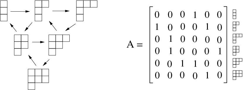
To do this, we imagine a directed graph with vertices corresponding to the allowed profiles. An edge leads from profile to profile if can be obtained from by adding one box. This is illustrated in figure 9. If we take the adjacency matrix of this graph, and raise it to power , the matrix elements are equal to the number of ways of getting from one profile to another using steps. In this way, we can obtain the value of needed in equation 19. This is the number of ways to get from to (the profile of ) using steps. Similarly, we can obtain , which is the number of ways of getting to by starting with the profile of and making steps. Thus, after computing the relevant powers of , we can then efficiently compute each using equations 19 and 20.
Given our table of cutoffs, the procedure for computing is a simple iteration. Suppose we know . To obtain we compare the register of qubits to the relevant cutoffs
to determine which row the box is added to. If the box is added to row , then we decrement (unless ) and increment .
The and registers together with the ancilla qubits containing encode the locations of boxes and . Thus, we can perform the transformation , as specified by equations 14 and 21 using a quantum circuit that acts only on these qubits. More specifically, this quantum circuit performs a unitary transformation on the and registers that depends on the content of the ancilla qubits. The ancilla qubits themselves are not transformed.
The unitary transformation performed on the and
registers is one which rotates between the encodings of a pair
standard Young tableaux which differ by having boxes and
swapped. is not injective, but the number of bitstrings
which encode these two tableaux are approximately equal. We illustrate
this with an example. Suppose
![[Uncaptioned image]](0807.4688v2/eightbox.png) . Consider the following
pair of standard Young tableaux
. Consider the following
pair of standard Young tableaux
The total number of standard Young tableaux of shape whose first five boxes appear in the configuration shown at left is the same as the number of standard Young tableaux of shape whose first five boxes appear in the configuration shown at right. This is because this number depends only on the shape of the dashed region. Returning to the general case, we see that swapping a pair of labelled boxes can never change the shape of the dashed region. By the definition of , the fraction of the possible bitstrings for registers and that encode a given configuration of boxes and is proportional to the fraction of Young tableaux of shape in which the boxes are in that configuration. Hence, number of bit assignments for registers and that encode a given configuration is equal to the number that encode the configuration in which boxes and are swapped, up to rounding. Thus we can always make some canonical matching between the bitstrings encoding the two configurations. The encoded version of transformation 14 is then to unitarily rotate between the current bitstring and its canonical matching.
In the case of Jones polynomials, we specified the canonical matching in equation 12. Here due to greater complexity we do not specify any formula for the matching. Instead, while computing all the cutoffs, one can at the same time make arbitrary choices for the corresponding matchings and write them down. A complete lookup table of these choices can be stored using polynomially many bits because . Given the choices of matchings, one can then use equation 14 to calculate all the matrix elements of . This matrix has polynomial dimension since it acts only on the two registers qubits each plus the ancillas encoding . It can therefore be implemented by an efficient quantum circuit using the method of [15]. After performing the unitary transformation, can be uncomputed.
As mentioned above, because of rounding, the number of bitstrings encoding the swapped and unswapped pair of boxes are not precisely equal, only approximately equal. Thus our canonical matching will in general have a small number of unpaired bitstrings encoding one of the two tableaux. As we did for Jones polynomials we define the unitary transformation to act as the identity on these excess bitstrings outside of the matching. By an analysis essentially identical to that in section 4 one can see that choosing logarithmic in the number of crossings suffices to ensure that these unmatched bitstrings form a small enough fraction so that their effect on the trace of the circuit is negligible.
By the above procedure we can construct an efficient quantum circuit for satisfying equation 21 for any and any . By concatenating these, we can thus obtain a quantum circuit for for any of polynomially many crossings. If is the link obtained by taking the trace closure of with each strand oriented downward then the corresponding HOMFLY polynomial is given by the Markov trace
For any we can estimate the normalized trace of to polynomial precision using the standard one clean qubit algorithm for trace estimation. Thus, we can estimate the HOMFLY polynomial by classically sampling from the possible Young diagrams according to the distribution
and estimating the corresponding normalized trace
for each sampled.
To do this we need to compute the values of and for each allowed . It is not hard to see that the allowed -box Young diagrams are in bijective correspondence with the allowed profiles. Thus for fixed and , the number of values of we need to compute is independent of . It is clear by equation 17 that each can be classically computed in polynomial time. Similarly, for fixed and , there are only different values of to compute. , thus each can be computed in polynomial time using the algorithm for computing described earlier.
7 Conclusion
In this paper we have shown that one clean qubit computers can in polynomial time obtain additive approximations to the Jones and HOMFLY polynomials of the trace closure of braids at arbitrary roots of unity. This generalizes the result of [18] which showed that one clean qubit computers can efficiently approximate the Jones polynomial of the trace closure of braids at the fifth root of unity. In [18] it was also shown that this problem is DQC1-complete. The completeness proof is based on the fact that the image of the path model representation modulo global phase is dense in . By the results of [7], this density result holds also for all other than 1,2,3,4, and 6, and similar density results hold for the Jones-Wenzl representation. Thus it is natural to conjecture that DQC1-completeness extends to Jones polynomials beyond and to HOMFLY polynomials. DQC1-completeness would imply that the additive approximations achieved by the algorithms here cannot be achieved in polynomial time by classical computers unless DQC1 P. Such completeness questions provide a promising direction for further research.
Another direction is to generalize the algorithm even further. For evaluating the Jones polynomial when is not a root of unity, the relevant representation of the braid group is nonunitary. In [2], Aharonov et al. give a general quantum algorithm to approximate Jones polynomials at all values of and to evaluate Tutte polynomials. They achieve this by interacting the computational qubits with an “environment” of ancilla qubits thereby inducing nonunitary dynamics on the computational qubits. It would be interesting to see whether similar techniques can be carried over to the one clean qubit model.
8 Acknowledgements
We thank Peter Shor for useful discussions. During the research and writing of this paper SJ was at Center for Theoretical physics at MIT, the Digital Materials Laboratory at RIKEN, and the Institute for Quantum Information at Caltech. SJ thanks these institutions as well as the Army Research Office (ARO), the Disruptive Technology Office (DTO), the Department of Energy (DOE), Franco Nori and Sahel Ashab at RIKEN, and John Preskill at Caltech. PW gratefully acknowledges support from NSF grants CCF-0726771 and CCF-0746600. PW would like to thank Eddie Farhi’s group for their hospitality and the W. M. Keck Foundation for partial support.
Appendix A Jones Polynomials from HOMFLY polynomials
As shown in figure 6, a Young tableau corresponds to a process by which a Young diagram is built up by adding one box at a time. If then the Young diagram has two rows (although at some steps the second row may be empty). This process can therefore be completely described by listing the difference between the number of boxes in the first and second rows at each step. The values of this difference correspond to the rungs of the ladder in the path model, as illustrated in figure 10. The values appearing in the path model representation, as defined in section 2, can be rewritten as follows.
Thus, comparing the path model representation to equation 14 shows that
| (23) |


As shown in section 5 of [20], the weights in the Markov trace for the Jones-Wenzl representation simplify substantially in the case . Specifically, the weights given in equation 17 simplify to
where is the number of boxes in the top row of minus the number of boxes in the bottom row of plus 1. By the correspondence of figure 10, is the final rung of the corresponding path. The Markov trace of the Jones-Wenzl representation of the identity braid is 1. Thus
and so
where the sum over is over all Young diagrams of boxes and 2 rows such that . Comparison with equation 3 shows that the weighted traces appearing in the Jones and HOMFLY polynomials are weighted identically in the case . This fact and equation 23 show that for any braid ,
| (24) |
where is the sum of the exponents appearing in when written in terms of the generators . Substituting equation 24 into equation 13 and simplifying yields
where is the directed link obtained by taking the trace closure of the braid . is minus the writhe of . Thus, comparison with equation 2 shows
The sign discrepancy is itself a link invariant, and is therefore inconsequential. To show this we use Markov’s theorem, which states that the oriented link obtained by taking the trace closure of braid is equivalent to the oriented link obtained by taking trace closure of braid if and only if can be transformed into by some finite sequence of the two Markov moves shown in figure 11 (and their inverses). It is easy to see that the factor is invariant under both Markov moves for all braids and is therefore an invariant of the corresponding trace closures.
References
- [1] Dorit Aharonov and Itai Arad. The BQP-hardness of approximating the Jones polynomial. arXiv:quant-ph/0605181, 2006.
- [2] Dorit Aharonov, Itai Arad, Elad Eban, and Zeph Landau. Polynomial quantum algorithms for additive approximations of the Potts model and other points of the Tutte plane. arXiv:quant-ph/0702008, 2007.
- [3] Dorit Aharonov, Vaughan Jones, and Zeph Landau. A polynomial quantum algorithm for approximating the Jones polynomial. In Proceedings of the 38th ACM Symposium on Theory of Computing, 2006. arXiv:quant-ph/0511096.
- [4] Andris Ambainis, Leonard Schulman, and Umesh Vazirani. Computing with highly mixed states. Journal of the ACM, 53(3):507–531, May 2006. arXiv:quant-ph/0003136.
- [5] H. Boerner. Representations of Groups. North-Holland, 1963.
- [6] Animesh Datta, Steven T. Flammia, and Carlton M. Caves. Entanglement and the power of one qubit. Physical Review A, 72(042316), 2005. arXiv:quant-ph/0505213.
- [7] M. H. Freedman, M. J. Larsen, and Z. Wang. The two-eigenvalue problem and density of Jones representation of braid groups. Communications in Mathematical Physics, 228(1):177–199, 2002. arXiv:math.GT/0103200.
- [8] Michael Freedman, Alexei Kitaev, and Zhenghan Wang. Simulation of topological field theories by quantum computers. Communications in Mathematical Physics, 227:587–603, 2002.
- [9] Michael Freedman, Michael Larsen, and Zhenghan Wang. A modular functor which is universal for quantum computation. arXiv:quant-ph/0001108, 2000.
- [10] Joel Hass, Jeffrey Lagarias, and Nicholas Pippenger. The computational complexity of knot and link problems. Journal of the ACM, 46(2):185–211, 1999. arXiv:math.GT/9807016.
- [11] F. Jaeger, D. L. Vertigan, and D. J. A. Welsh. On the computational complexity of the Jones and Tutte polynomials. Mathematical Proceedings of the Cambridge Philosophical Society, 108:35–53, 1990.
- [12] Vaughan F. R. Jones. A polynomial invariant for knots via von Neumann algebras. Bulletin of the American Mathematical Society, 12:103–111, 1985.
- [13] E. Knill and R. Laflamme. Power of one bit of quantum information. Physical Review Letters, 81(25):5672–5675, 1998. arXiv:quant-ph/9802037.
- [14] E. Knill and R. Laflamme. Quantum computating and quadratically signed weight enumerators. Information Processing Letters, 79(4):173–179, 2001. arXiv:quant-ph/9909094.
- [15] Michael A. Nielsen and Isaac L. Chuang. Quantum Computation and Quantum Information. Cambridge University Press, Cambridge, UK, 2000. (See section 4.5.).
- [16] David Poulin, Robin Blume-Kohout, Raymond Laflamme, and Harold Ollivier. Exponential speedup with a single bit of quantum information: Measuring the average fidelity decay. Physical Review Letters, 92(17):177906, 2004. arXiv:quant-ph/0310038.
- [17] C. A. Ryan, J. Emerson, D. Poulin, C. Negrevergne, and R. Laflamme. Characterization of complex quantum dynamics with a scalable NMR information processor. Physical Review Letters, 95:250502, 2005. arXiv:quant-ph/0506085.
- [18] Peter W. Shor and Stephen P. Jordan. Estimating Jones polynomials is a complete problem for one clean qubit. Quantum Information and Computation, 8(8/9):681–714, September 2008. arXiv:0707.2831.
- [19] Edward Witten. Quantum field theory and the Jones polynomial. Communications in Mathematical Physics, 121(3):351–399, 1989.
- [20] Pawel Wocjan and Jon Yard. The Jones polynomial: quantum algorithms and applications in quantum complexity theory. Quantum Information and Computation, 8(1/2):147–180, January 2008. arXiv:quant-ph/0603069.