IPPP-08-56
CPT-08-112
Searching for Nambu - Goldstone Bosons at the LHC
Athanasios Dedes, Terrance Figy, Stefan Höche,
Frank Krauss, and
Thomas E. J. Underwood
aDivision of Theoretical Physics, University of Ioannina, Ioannina,
GR 45110, Greece
bInstitute for Particle Physics Phenomenology, University of
Durham, DH1 3LE, UK
cMax-Planck-Institut für Kernphysik, Saupfercheckweg 1, 69117
Heidelberg, Germany
ABSTRACT
Phenomenological implications of a minimal extension to the Standard Model are considered, in which a Nambu-Goldstone boson emerges from the spontaneous breaking of a global symmetry. This is felt only by a scalar field which is a singlet under all Standard Model symmetries, and possibly by neutrinos. Mixing between the Standard Model Higgs boson field and the new singlet field may lead to predominantly invisible Higgs boson decays. The “natural” region in the Higgs boson mass spectrum is determined, where this minimally extended Standard Model is a valid theory up to a high scale related with the smallness of neutrino masses. Surprisingly, this region may coincide with low visibility of all Higgs bosons at the LHC. Monte-Carlo simulation studies of this “nightmare” situation are performed and strategies to search for such Higgs boson to invisible (Nambu-Goldstone boson) decays are discussed. It is possible to improve the signal-to-background ratio by looking at the distribution of either the total transverse momentum of the leptons and the /, or by looking at the distribution of the azimuthal angle between the / and the momentum of the lepton pair for the - and Higgs-boson associated production. We also study variations of the model with non-Abelian symmetries and present approximate formulae for Higgs boson decay rates. Searching for Higgs bosons in such a scenario at the LHC would most likely be solely based on Higgs to “invisible” decays.
1 Introduction
In a seminal paper published in 1962, Goldstone, Salam and Weinberg [1] proved that the physical particle spectrum of a theory in which a continuous, global symmetry is spontaneously broken must contain one massless, spin-zero particle for each broken symmetry. Massless particles of this type, today called Nambu-Goldstone bosons (NGB), were first theoretically discovered in particular models by Goldstone [2] and Nambu [3]. In the following, they will collectively be denoted by the symbol . NGBs have the peculiar property that they couple to the divergence of the current associated with the symmetry that is broken. This coupling has a strength which is inversely proportional to the scale of symmetry breaking ,
| (1.1) |
This form of interaction is invariant under the shift transformation, , where is an angle that parameterizes different vacuum field configurations. Since NGBs typically are amongst the lightest particles in a theory a large fraction of the other particles can decay into them through eq. (1.1). For this decay to occur, these other particles, possibly scalars and/or quarks and leptons, must be charged under the same spontaneously broken global symmetry. It was first proposed by Suzuki and Schrock [4] that if the Standard Model (SM) Higgs boson mixes with such a new scalar particle then it must have a decay channel into a pair of NGBs () provided that the scale is of the order of the electroweak gauge boson masses, . If such a Higgs boson decay exists then it should be searched for at colliders.
The basic idea underlying this article is the existence of an additional global “phantom” symmetry, (P stands for “Phantom”), that is spontaneously broken at some scale . Then following eq. (1.1), will couple to all fermions () that are charged under since . This coupling will be proportional to . In the literature, there are three famous types of Nambu-Goldstone bosons: axions [5], familons [6] and majorons [7] and their associated broken symmetries are the Peccei-Quinn symmetry [8], and the family and lepton number symmetry, respectively. In the former two cases the global symmetry is carried by both quarks and leptons and in the latter case by leptons only. However, considerations of energy loss in stars, supernovae and/or in terrestrial collider experiments [9] conclude that GeV in these popular cases. This bound constrains the decays of Higgs particles into the NGBs of the aforementioned models to be completely unobservable at colliders. Recently, a Majoron model has been considered where lepton number is spontaneously broken at the electroweak scale but in accordance with astrophysical bounds [10], however we will not consider this class of models here. A different situation arises if we assume that such additional NGBs, if existent, must exclusively couple to phantom (SM gauge singlet sector) fields.
It is important to note that the requirement of renormalizability poses some constraints on such a hypothetical phantom sector. In particular, it demands that the only places where a phantom sector can make connections to the SM are the Yukawa interactions of neutrinos and Higgs bosons and the “mass” term. Therefore, the only relevant phantom sector fields are a right-handed fermion (possibly coming in three copies) and (in general complex) scalar fields. This immediately triggers some thought on implications for neutrino masses. For them, there are two possibilities: Majorana or Dirac masses. The Majorana see-saw mechanism [11] in fact is nothing but a type of phantom sector. However, as already discussed, in the simplest models the possible spontaneously broken global symmetry is lepton number – clearly not a purely phantom sector symmetry. So, what about the Dirac case? Sticking to the same principle that leads to suppressed neutrino masses in the Majorana see-saw scenario, an analogous non-renormalizable operator can be constructed. It reads
| (1.2) |
In the model proposed in this article, some (purely phantom sector) symmetry , prevents the interaction from providing neutrinos with electroweak-scale masses. Then, eq. (1.2) results in acceptably small Dirac neutrino masses after spontaneous symmetry breaking of (and the extended SM gauge group ) at provided that GeV. Here, the field (where ) is the standard model Higgs doublet and “” denotes the inner product within or . A renormalizable model resulting in the effective operator of eq. (1.2) was first built by Roncadelli and Wyler [12]. It has been recently shown in ref. [13] that this model would lead to successful baryogenesis via Dirac leptogenesis [14, 15, 13] if TeV.
It is worth noting that this particular NGB evades many bounds applying to other species of NGB since the only fermions transforming under are the , and the coupling between the NGB and the neutrinos is proportional to . This is too small to affect neutrino flavour oscillations through [16].
It is not unreasonable to suppose that the effects of the phantom sector may already have been seen 11 1 One should also notice that, like s, the three right-handed neutrinos being SM-gauge singlets are the only light fermions that obey the shift invariance, where is a Grasmann-type parameter. It may be tempting to interpret the s as Goldstinos of an (with being the number of flavours) supersymmetric phantom sector where the s belong to the same supermultiplet. in experiments revealing that neutrinos have small masses.
The existence of such a phantom sector may also be responsible for electroweak symmetry breaking. This has recently been emphasized by Patt and Wilczek [17] and also by the authors of ref. [13]. Their argument is based on the fact that no symmetry principle can forbid the mixing of the Higgs sector with the phantom sector through the renormalizable link operator
| (1.3) |
Eq. (1.3) suggests that the phantom sector field triggers spontaneous electroweak symmetry breaking, i.e. GeV once it develops a vacuum expectation value (vev), . This holds true even in the absence of any tree-level Higgs mass term, [18, 19, 20]. Furthermore, it is exactly the mixing term of eq. (1.3) that causes the Higgs boson to decay into a pair of NGBs, . Since the s interact only very weakly with matter, this decay effectively constitutes an invisible decay of the Higgs boson.
Of course, this discussion could be generalized to non-Abelian groups. However, for simplicity here and onwards the simplest group is assumed. The Noether current associated with this symmetry is . The phantom field can be expanded about its vev in the usual fashion,
| (1.4) |
Using eq. (1.1) the interaction between the massive Higgs boson and the NGB is found to be . The scalar potential is composed of the usual quadratic and quartic terms for and as well as the link term of eq. (1.3). It is independent of i.e. , where is the neutral field component of the -Higgs doublet. The fields and are rotated to their physical mass eigenstates, , with an orthogonal rotation matrix (CP-conservation is assumed). After setting particles on their mass shell, becomes [4],
| (1.5) |
where in this minimal scenario22 2 The link term of eq. (1.3) also gives rise to quartic couplings which are given in Fig. 11 of Appendix A. These couplings contribute to the decay, . However, the decay rate for this channel is on the order of GeV or less for benchmark scenarios considered in this paper. Hence, they will be completely neglected in the analysis presented here.. In this case the rank-2 matrix contains one mixing angle . Following the notation of ref. [13], it will be fixed by and . The limit implies , i.e. no mixing between the SM-Higgs and the phantom sector scalar fields. Obviously, in this limit the Standard Model is recovered. This article assumes a convention where . Trading the vev of with the more familiar , the free parameters of the model read
| (1.6) |
Eq. (1.5) is the equation underlying all phenomenological analyses in this paper. It describes Higgs boson decays to the almost sterile NGB particles. There exists an extensive body of literature, which addresses various techniques for discovering an invisible Higgs boson at colliders. They can be assembled in three main strategies:
- •
Studying the recoil of the -gauge boson in the associated production process. Experimental results from LEP are summarized in [21] and simulations have been performed in [22]. A study for this process at the Tevatron has been performed in refs. [23, 24] with the result that the collider needs substantially more integrated luminosity to improve the current LEP exclusion limit. Parton level simulation studies for the LHC exist in Refs.[25, 26, 24]. Further hadron level/detector simulation studies for the LHC are currently under way [27, 28].
- •
- •
Central exclusive diffractive production has been studied for a particular model in ref. [31].
It should be noted that in all the above analyses only models with only one Higgs boson decaying completely invisibly were considered.
In this article the focus will be put on the first two search channels, namely production and VBF. In both cases, the coupling of the Higgs to the gauge bosons is crucial. In the model considered here, only the SM-like scalar field , belonging to the Higgs-doublet, couples to vector bosons . The corresponding SM coupling constant is rescaled with the mixing angle such that
| (1.7) |
Since the matrix is real and orthogonal, its elements are smaller than unity. This immediately implies that all Higgs production cross sections and/or decay rates (to SM particles) in this model are suppressed relative to the SM by a factor . However, because of the orthogonality condition, . Therefore, if for example is invisible then the other Higgs tends to be visible and vice-versa. Is this a no-lose theorem for a Higgs boson discovery in this type of model? This is one of the questions to be addressed in this paper.
More specifically, in this article the following two questions will be discussed:
- Q1:
Is there any window in the parameter space (1.6) where LEP failed to exclude both Higgs-bosons for GeV ?
- Q2:
Is there any (natural) window in the parameter space (1.6) where both Higgs bosons would hide undetected at LHC?
In this context “natural” means that the theory has a positive definite potential, with perturbative (non-trivial) couplings up to a high cut-off scale GeV, where the mechanism for naturally light neutrino masses may be expected [recall eq. (1.2)]. Therefore, we begin our analysis with Section 2 where stability and triviality bounds are analyzed and plotted together with electroweak -parameter constraints. In Section 3, we answer question Q1. We derive analytical formulae for the Higgs boson to “visible” () and “invisible” () decay rates and plot predictions of the model against experimental LEP exclusion data for Higgs masses less than, approximately, 114 GeV. A possible scenario explaining the LEP Higgs boson excess is also discussed in this section. In Section 4, we extend the region of validity of () and () to heavier Higgs boson masses, and justify five benchmark points. Next, in subsections 4.1-4.2, we perform a detailed Monte-Carlo simulation for signals at these points and their backgrounds, and we discuss possible strategies useful for further theoretical and experimental consideration. Furthermore, in Section 5, extensions of the Abelian to non-Abelian phantom sectors and some consequences relevant for Higgs boson phenomenology at the LHC are discussed. A discussion of our findings together with some remarks for alternative scenarios is presented in Section 7. In Appendix A, we display the relevant Feynman rules of the Abelian model.
2 Stability and Triviality Bounds
In the minimal phantom model, the set of physical parameters in eq. (1.6) can be written33 3 We adopt the notation of ref. [13]. in terms of the renormalization group running parameters , , and :
| (2.1) | |||||
| (2.2) | |||||
| (2.3) |
with GeV. Notice that in the limit where both the phantom sector completely decouples from the SM scalar sector. Also, note that depends quadratically on and the Higgs boson masses. This implies that in the case of non-zero Higgs mixing there is always an upper bound on if the theory is required to remain perturbative. For example, if and GeV then . In all of our plots only the case is considered although, as already explained, higher values of would further reduce the number of visible Higgs events.
There are two44 4 The unitarity constraint here is avoided by assuming that all quartic couplings are in a perturbative region, . classic, “theoretical” constraints on models that have been worked out numerous times in great detail for the SM and in many of its extensions [32]. Firstly, the triviality constraint is essentially the requirement that the couplings in eq. (2.1) - eq. (2.3) stay perturbative up to a certain scale . Secondly, the vacuum stability constraint demands that the potential is bound from below up to a scale . Applying both constraints yields GeV, where we recall the discussion following eq. (1.2). The vacuum stability bound can be reduced to the requirement
| (2.4) |
at all scales .
The running parameters are defined at the scale and then evolved up to higher scales with the following 1-loop renormalization group equations [33, 34]
| (2.5) |
Here, , and are the and gauge couplings, respectively, and is the top quark Yukawa coupling. We ignore all other Yukawa couplings because their effect in the running is negligible. The equations for , and are well known [35] and are left out for brevity. It is worth noticing that the parameter is multiplicatively renormalized at one loop. Although there is no particular reason for , if this is the case at one energy scale then this will remain true at all energy scales.
Fig. 1 shows the light Higgs boson mass vs. plane for where the background colours show the scale of new physics required either by positivity or triviality (whichever is lower). The curved contour shows the 95% C.L. upper limit on the combined Higgs boson masses from precision electroweak data (see corresponding formula in ref. [13]). Fig. 1 should be compared with Fig. 5 of Section 4, to see the correspondence between easily accessible regions at the LHC and regions with a potentially high effective theory cut-off. The light (light green) shaded parameter region of Fig. 1 is what we will coin the natural region throughout this paper.

3 LEP searches
The LEP experiments searched first for visible Higgs boson events in the Higgsstrahlung process with the Higgs boson decaying to -quarks and leptons in final state stemming from the boson decay. They presented [36] 95% C.L. upper limits for a parameter (in their notation ), defined as the ratio of the number of Higgs boson events expected in any given model to the number expected in the Standard Model for a Higgs boson with an identical mass, as a function of the Higgs boson mass. An important point to note in this context is that only counts “visible” events. In particular, the data on decays to -quarks will be used in the following. Then the parameter translates into
| (3.1) |
where , are the remnants associated with the production of a or (the SM Higgs boson) and could be in principle either , or , but not . However, in the framework of the particular model studied here, another possibility is that . Exclusion limits in this case have been presented in [36].
The four LEP experiments [37] also performed searches for acoplanar jets (as signal for ) or leptons (as signal for ), with , apart from the DELPHI-collaboration which also used ’s in the final state. In all cases, the emergence of invisible decay products of the Higgs boson is identified with the production of missing energy (/). Their study resulted in an upper limit on the branching ratio of as a function of the Higgs mass, multiplied by the production cross-section normalized to the rate expected from a SM Higgs decaying completely invisibly. In our case, this limit places constraints on the parameter
| (3.2) |
where again , is the SM Higgs boson and are the remnants associated with the production of or at LEP.
A further important constraint comes from the OPAL collaboration who performed a model-independent analysis of the Higgs sector at LEP [38]. They searched for the generic process where is a completely neutral (and hence invisible) scalar boson. Since this analysis is independent of the eventual fate of the Higgs candidate it bounds the parameter
| (3.3) |
as a function of the Higgs boson mass. In this model and .
Particularly simple expressions may be derived for and in the minimal phantom scenario provided that the narrow width approximation may be assumed and that the Higgs boson to off-shell gauge boson decay modes may be neglected. Our analytical findings closely follow the model-independent analysis of ref. [39]. Consider the case where in eq. (3.1). For simplicity let us assume that the decay is kinematically forbidden, i.e. . In this case . Applying this to eq. (3.1) in the LEP search region, and after some algebra we arrive at
Firstly, notice that the number of Higgs boson events where the Higgs boson decays to (or indeed any other visible mode) are always suppressed relative to the SM prediction in which for this particular Higgs boson mass region. Secondly, the number of visible Higgs boson events decreases in the limit . Note also that if , receives an additional suppression.
The importance of the Higgs boson to invisible decay and of model-independent Higgs boson analyses are highlighted when we consider the example and where we obtain for GeV. In principle, this is within the region allowed by LEP “visible” Higgs search data [36] which excludes for Higgs masses in the range .
This could have been a “nightmare” scenario; LEP would have completely missed the Higgs sector! Fortunately, this nightmare is averted by both the LEP Higgs boson to invisible searches and the OPAL model-independent Higgs boson search, because the former, for instance, sets bounds on . In the relevant LEP mass region, ,
| (3.4) | |||||
| (3.5) |
Setting implies that . LEP searches for invisible Higgs bosons exclude for masses below 110 GeV, GeV. Therefore, it is unlikely that there are two invisible Higgs bosons in the LEP search region with masses GeV. This answers question Q1 posed in the introduction.
In addition, using the model-independent analysis of OPAL [38], GeV is excluded for . Since either or for any given , OPAL excludes the case where both GeV and GeV, independently of how the Higgs bosons actually decay.
It is interesting to note that one Higgs boson could still be hidden in the LEP search region even with these strong constraints, while the other Higgs boson then would wait for its discovery in the allowed region out of reach of LEP.
 |
 |
The results of a detailed analysis of this model, including visible, invisible and model-independent LEP bounds [36, 37, 38] are summarised in Fig. 2. This numerical analysis confirms the analytical findings above. With , a light Higgs boson () with a mass as low as 65 GeV could have escaped unobserved at LEP if . For the same range of the other Higgs () is constrained to be heavier than 114 GeV. From inspection of Fig. 2 we can define a LEP-allowed benchmark scenario B1 for the phantom model presented here, namely:
| , | |||||
| , | (3.6) |
In this case one Higgs boson is buried, undiscovered in the LEP search region due to the small values of and which have to satisfy following eq. (3.4). The other, heavier Higgs has and . With this set of parameters, very few events are SM-like decays into “visible” final states and instead decays mainly into “invisible” NGBs. This scenario could well be classed as a (LEP) nightmare!
As yet, no combined LEP limits exist on invisibly decaying Higgs bosons with masses below GeV. Therefore, for GeV the limits presented here are based on the individually published results from each experiment. However, some of the individual studies do not cover the whole Higgs mass range considered here and so the best available limit is used for any given Higgs mass. This is one of the causes of the sharp edges in Fig. 2. Clearly, a future combined LEP analysis may well exclude the benchmark B1 which lies close to being ruled out by ALEPH [37] which considered Higgs masses down to GeV for which is excluded.
3.1 A digression: 2.3 LEP Higgs search excess
The LEP experiments established a small, 2.3 effect in their Higgs boson searches corresponding to a Higgs boson mass of about 98 GeV [40]. Explaining this excess would require a value of , ruling out a Standard Model Higgs boson as plausible explanation. It is possible to provide a candidate Higgs boson in the phantom model discussed in this publication, which would have produced such an effect in the LEP data. Fig. 3 shows the allowed region in the vs. plane for GeV. The allowed region is tightly constrained because of the searches for invisible Higgs bosons at LEP in this mass region. At the relatively small values of still allowed, the main reason for such a small value of is Higgs mixing rather than the extra invisible decay mode suppressing the Higgs branching ratio.


Fig. 4 shows the constraints on this region of parameter space coming from considering the triviality and positivity of the potential. For a suitably heavy GeV, most of the region suggested by the LEP excess is described by a theory which could be valid to scales as high as GeV. When , as () the values of and tend to 0. Looking at eqs. (2.5) it is apparent that small values of and will be relatively stable under renormalization group evolution since, for example, is multiplicatively renormalized. Higgs masses around the electroweak scale are maintained in this limit because whilst . However, because the and sectors are almost decoupled so that potentially destabilizing diagrams with a heavy will be proportional to and not greatly affect the mass of . Of course, the model is still quadratically sensitive to a high cut-off scale and thus still possesses the hierarchy problem of the SM.
Note that the second Higgs boson mass is restricted by the upper limit on Higgs boson masses from precision electroweak data [13], however for GeV the whole region suggested by the LEP excess is free from this constraint. Clearly further data would be required before this effect could be taken more seriously.
In the next chapter we will address the question of whether the LHC has the sensitivity required to discover these scenarios, in particular the potential nightmare B1. The possible existence of other challenging scenarios with heavier Higgs bosons will also be examined.
4 LHC: expectations and strategic searches
In the LHC search region, the parameters and can be defined by expressions similar to those in eqs. (3.1) and (3.2), respectively, with the obvious replacement of the electron/positron initial state to a proton/proton initial state and etc.. Two categories for the ratios may be distinguished: (a) a region where and decays dominantly into and (b) a region where and the decays dominantly into a gauge boson pair, , with .
In case (a), and under the assumption that gauge bosons are produced on-shell, analytical approximations for are identical to those studied in the previous chapter. On the other hand, assuming a common gauge boson mass , in region (b), we obtain
where , and . The last term in eq. () is the contribution from the heavy Higgs boson decay [34, 41]. Furthermore, and . Imposing some constraints to this analysis (see section 2), the mode will not be important in further discussions.
It is apparent from eq. () that a certain suppression of the observable rates () is always present. Its origin is twofold. Firstly, the couplings between the and SM fields are always suppressed because of the mixing matrix . Secondly, the decay widths of the Higgs bosons are enhanced by the extra decay mode . The contribution of this additional decay mode is increased at large and for and the suppression of visible events is always more than 90% for GeV. However, as we have already remarked in section 2, high values of result in non-perturbative couplings and will therefore not be considered in this article.
What then would be a nightmare scenario for the LHC? At present both the ATLAS and CMS collaborations have performed studies, at detector simulation level, to explore the discovery potential of their apparatus for both SM-like Higgs bosons which decay to visible final states, see e.g. [42], and Higgs bosons decaying to invisible final states, for example [30, 28]. These studies are sensitive to the ratios and as functions of the Higgs boson mass. For example, looking at the simulation results for the LHC with integrated luminosity we estimate (with naïve scaling) that it would be difficult to discover a visibly-decaying Higgs if signal event rates were 30%(20%) of that expected in the SM (). Furthermore, studies of the sensitivity of the ATLAS detector55 5 Similar studies exist for the CMS detector [43]. to invisibly decaying Higgs bosons suggest that after integrated luminosity ATLAS could exclude Higgs bosons with at 95% C.L. [30, 28].
To further illustrate the necessity of the Higgs boson to invisible searches in this minimal phantom scenario, in Fig. 5 areas on the vs. plane are plotted where and/or . These limits define naïve regions, where Higgs bosons will experimentally be accessible at the LHC, either in visible or invisible search channels. Clearly at this stage in this study these limits are assumptions, and in fact the true experimental reach of the LHC will not be known until after it has been running for some time and predictions for the levels of backgrounds have been confirmed (or not). These assumptions do, however, serve as a good first estimate on which to justify the further study undertaken here.
In producing Fig. 5 all Higgs boson decay modes including decays to off-shell vector bosons have been considered. Different colours indicate regions where either one, both or no Higgs bosons can be seen in different channels. It is clear that a truly challenging region for LHC region remains where and . This motivates the further more detailed Monte Carlo analysis in the later sections of this article, which probe more carefully the possibility of discovering a Higgs boson in the invisible search channel when .

Using equations (3.4) and (3.5) it is easy to see that . The following no-lose theorem then exists: If experiments can discover a Higgs boson over the whole range of down to or over the whole range of down to then at least one Higgs boson should be found.
Without real data, estimates of the capabilities of experiments like ATLAS and CMS may easily be too optimistic or too pessimistic. Therefore in this publication, a constructive approach is taken. The phantom model has been added to the Monte Carlo event generator S HERPA [44], ready to be used when real data arrive. For now Fig. 5 may be used to define additional benchmark scenarios, some in potentially nightmarish regions, and these points can be studied in more detail. The particular scenarios are displayed in Table 1.
| Benchmark | (GeV) | (GeV) |
|---|---|---|
| B2 | 112 | 130 |
| B3 | 140 | 165 |
| B4 | 160 | 190 |
| B5 | 185 | 190 |
The LO branching ratios for both Higgs bosons are presented in Table 2. These ratios are in agreement with the analytical LO expressions in eq. () and Fig. 5, and the discussion following them. The most optimistic benchmark point is B1 and the most challenging one is B5.
| Benchmark | Higgs | (GeV) | ||||
|---|---|---|---|---|---|---|
| B1 | 0.041 | 0.694 | – | – | 99.222 | |
| 0.051 | 3.567 | 0.289 | 0.020 | 95.533 | ||
| B2 | 0.117 | 0.958 | 0.059 | 0.003 | 98.823 | |
| 0.183 | 0.697 | 0.348 | 0.042 | 98.784 | ||
| B3 | 0.229 | 0.593 | 0.779 | 0.103 | 98.408 | |
| 0.490 | 0.319 | 23.769 | 0.498 | 75.339 | ||
| B4 | 0.387 | 0.393 | 12.217 | 0.396 | 86.904 | |
| 1.066 | 0.166 | 36.597 | 10.313 | 52.879 | ||
| B5 | 0.921 | 0.188 | 36.500 | 6.787 | 56.475 | |
| 1.066 | 0.166 | 36.597 | 10.31 | 52.879 |
Prospects for discovering the Higgs bosons in the various benchmark scenarios B1-B5 at the LHC will be studied in the following. Theoretical vacuum stability and triviality bounds as well as bounds from fitting electroweak (EW) observables have already been presented in Section 2. All benchmark scenarios selected in Table 1 satisfy the EW constraints and in some the effective theory may be valid even to scales as high as the Planck scale.
4.1 -production
The first search channel for an invisibly decaying Higgs boson at the LHC considered here is the associated production of a and a Higgs boson, where the decays leptonically. This ensures that a corresponding event can be triggered. The backgrounds to this process include , , and production with corresponding decays, and fully leptonic production66 6 Note that, in all processes, off-shell effects, - interference etc. are fully included in the simulation.. It should be noted here that in principle some information on the rates can be obtained directly from data: for pairs, final states with four leptons may be reweighted with the corresponding branching ratio, in the case, different sign, different lepton pairs may be invoked. For the background, it may be possible to extrapolate from events where three leptons are seen to those where one lepton is lost, i.e. either outside the detector acceptance or undetected. For top-pair production, semi-leptonic events may help.
All processes have been simulated with S HERPA [44] in the following setup: In order to correctly model hard parton radiation S HERPA employs the multijet matrix element-parton shower merging procedure of [45]. Therefore, for all processes discussed here and in the next section, matrix elements with at least one and in most cases two additional jets have been added to the simulation. This ensures that the simulation correctly describes the important high- tails of various distributions. However, all cross sections quoted are, in principle, obtained at leading-order accuracy, with no -factors added to them. CTEQ6L parton distubution functions are used with [46]. is computed at two–loop accuracy. All scales are set according to the merging prescription of [45]. Jets have been defined in all cases through the algorithm [47]. The CKM matrix has been choosen to be diagonal.
We have simulated and analysed events with electrons in the final state; mostly identical numbers would have been obtained if we had specialised for muon pairs instead. Obviously, this difference would be of great importance if detector effects had been included as well77 7 We refrained from including full detector simulations, or any Gaussian smearing or electron-jet conversion “by hand” and concentrated on an analysis at the hadron level, including all effects of fragmentation, hadron decays, final state QED bremsstrahlung etc... However it should suffice to state that we quote final results for leptons . We also omitted all effects due to the underlying event because of the large uncertainties related to its modelling and the rather small impact it has on the observables we discuss.
The selection cuts listed in Ref. [28] have been applied. Thus we require:
- 1.
one lepton pair of the same kind with opposite charges, where each lepton individually satisfies GeV and ;
- 2.
GeV;
- 3.
GeV;
- 4.
a veto on jets with GeV, ;
- 5.
a veto on b-jets with GeV, ;
- 6.
GeV, where .
Additionally, we impose:
- 6.
;
- 7.
GeV.
For the various backgrounds listed above, cross sections before and after these additional selection cuts are listed in Table 3. Generation cross sections, selection cut efficiencies and the resulting selection cross sections for the signal in the different benchmark scenarios are given in Table 4. It should be stressed again that all cross sections quoted have been obtained at leading order accuracy.
| [fb] | 164 | 1.17 | 1.01 | 7.44 | 1.81 |
|---|---|---|---|---|---|
| only | 2.00 | 1.10 | 6.59 | 8.40 | 1.41 |
| GeV | 1.87 | 9.17 | 8.92 | 1.09 | 1.25 |
| GeV | 3.69 | 1.10 | 5.91 | 2.41 | 1.94 |
| jet veto | 1.64 | 2.13 | 3.53 | 2.00 | - |
| GeV | 1.54 | 1.95 | 2.74 | 1.19 | - |
| , GeV | 1.23 | 1.50 | 2.23 | 1.55 | - |
| [fb] | 2.02 | 1.75 | 2.25 | 1.15 | - |
| [fb] | 280 | 114.6 | 53.0 | 29.0 | 13.6 |
|---|---|---|---|---|---|
| only | 1.75 | 1.98 | 2.25 | 2.40 | 2.24 |
| GeV | 1.62 | 1.84 | 2.10 | 2.23 | 2.08 |
| GeV | 3.12 | 6.07 | 8.91 | 1.08 | 1.12 |
| jet veto | 3.00 | 5.66 | 7.85 | 9.29 | 1.08 |
| GeV | 2.88 | 5.49 | 7.64 | 9.08 | 1.06 |
| , GeV | 2.55 | 4.93 | 6.94 | 8.35 | 9.85 |
| [fb] | 7.15 | 5.65 | 3.68 | 2.42 | 1.34 |
The numbers from both Tables 3 and 4 suggest that the two most dangerous backgrounds to the signal are and production, with corresponding decays. Following our discussion above, however, it seems that the total cross sections and distributions related to these backgrounds can be directly extracted from data in the case or probably well extrapolated from measurements. After cuts we find that the backgrounds together account for roughly 8 fb, leaving us with signal-to-background ratios of the order of up to 1. We therefore conclude that it should be possible to find the signal in all five benchmark scenarios. However, we would like to stress here that more conclusive numbers can be obtained after a simulation at detector level only.
Such detector-level studies for an invisibly decaying Higgs boson have been for the ATLAS experiment [28] found signal–to–background ratios reaching up to . Although this is of the same order of magnitude as our results, there are several differences: First of all, in our simulation the S HERPA Monte Carlo event generator with multijet merging was used for both signal and background events, while the ATLAS study employed the P YTHIA [48] event generator for the backgrounds and the program h 2hv [49] for the signal. While S HERPA and P YTHIA are formally of the same accuracy there are a number of differences, like S HERPA multijet merging leading to an improved treatment of hard QCD radiation, and the full inclusion of spin correlations in S HERPA , which are not present in P YTHIA . This may have lead to a better separation of signal and background in S HERPA . On the other hand, in ATLAS’ simulation the couplings where assumed to have exactly the same strength as in the SM - which is not true for our analysis, where these couplings are reduced due to mixing effects. In addition, a 100% branching ratio of Higgs boson to invisible was assumed for the ATLAS simulation, again in contrast with our simulation, where the relevant branching ratio ranged between roughly 50% up to 100%. These two facets of the study, of course, enhance the signal–to-background ratio in the ATLAS study. Of course, there are further differences, like the missing underlying event in S HERPA , which has been included in the ATLAS study, like slightly different selection cuts, like a different choice of PDF (CTEQ5L in ATLAS, CTEQ6L in our study) and, most importantly, like the inclusion of detector effects through their fast detector simulation ATLFAST [50] in the ATLAS study that are totally absent in our case. To summarize: However different in detail the studies are, it is reassuring to see that in all cases this seems to be a feasible channel, at least at accumulated higher luminosities.
In addition to the findings above, cf. Tables 3 and 4 we have identified two further distributions that may be worthwhile to study in the channel:
- •
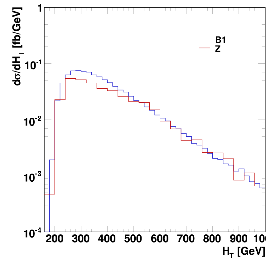
The total transverse momentum of the leptons and /, i.e. the total transverse momentum of the and candidates (see Fig. 6). This observable shows a significantly different behaviour between the signals and the backgrounds, where the signal tends to be more strongly peaked towards small values.
- •
The azimuthal angle between / and the momentum of the lepton pair (see Fig. 7). Here the signal tends towards a more back-to-back configuration of the and candidate. Seemingly, there is a significantly higher QCD activity in the backgrounds than in the signal, providing more jets for the -candidate pair to recoil against in the backgrounds.
These findings may help to further improve the signal-to-background ratio.


4.2 Vector Boson Fusion
The other production channel we consider for invisibly decaying Higgs bosons at the LHC is vector boson fusion (VBF). As the name suggests, in this process the Higgs boson is produced through the fusion of two vector bosons emitted by quarks inside the protons, which typically carry comparably large momentum fractions of the protons. Therefore, at leading order (tree-level) there is no colour exchange between the two protons, and it can be expected that the central rapidity region remains to a large extent empty apart from the decay products of the produced system. The quarks on the other hand will be deflected, typically by transverse momenta of roughly half the mass of the produced system. This gives rise to two hard jets, which, due to the invisible nature of the Higgs boson, are essentially the triggers in this analysis. The main background processes to be taken into account are the production of or bosons in association with two jets, which can originate either from QCD or through electroweak interactions, thus mimicking the topology of the VBF signal. In addition, top-pair production with subsequent semi-leptonic decays must be considered. Similar to the case of production, the lepton is then lost. Again, it is worth noting that it should be possible to extract information concerning the total rates of these backgrounds, even after selection cuts, directly from data. This is possible either by reweighting leptonic decays to those into neutrino pairs, or, with a somewhat larger error, by extrapolating the modes where the individual lepton is seen (in +jets or semileptonic top-pairs) into those regions where the lepton is lost. This is in analogy to the case discussed above.

We employ the basic cuts listed in Ref. [30], i.e. we require:
- 1.
two tagging jets with
- (a)
GeV, ,
- (b)
, ,
- (c)
GeV ,
- (d)
,
- (a)
- 2.
missing transverse momentum, GeV;
- 3.
no identified lepton, i.e. no lepton with
GeV in , - 4.
a central jet veto, i.e. no jets with
GeV, .
Additionally we impose:
- 5.
,
- 6.
.

The choice of the cut on the invariant tagging jet mass of GeV is motivated by the corresponding invariant mass spectrum shown in Fig. 8. We observe that the signal distribution crosses the background at GeV. Of course this statement sensitively depends on the model parameters chosen; however, the common feature of all scenarios is that the higher the invariant mass cut, the better the signal–to–bachground ratio. This is due to the fact that in a large fraction of background events the two tagging jets originate from QCD or the decay of weak gauge bosons.
After the above cuts the possibilities to check for the signal topology are limited in the VBF channel. Possible objects to be identified experimentally are the tagging jets, / and an eventually arising soft third jet. Therefore most observables show the same behaviour for signal and background, which is exemplified in the left panel of Fig. 9, showing the -distribution for the signal at benchmark point B1 and the background. In the right panel of Fig. 9 we show for the same scenario the distribution. It is clearly seen that for the background the third jet tends to be more central between the tagging jets, while for the signal it is rather forward or backward. This motivates the first of the additional cuts above.
For the various backgrounds listed above, cross sections before and after additional selection cuts, and the number of generated events are listed in Table 5. Signal cross sections before and after additional selection cuts are listed in Table 6.
| +jets (QCD+EW) | +jets (QCD+EW) | ||
| [nb] | 9.41 | 51.8 | 0.145 |
| tagging jets | 1.80 | 7.44 | 1.62 |
| 1700 GeV | 3.49 | 1.64 | 4.44 |
| GeV | 2.64 | 9.73 | 3.32 |
| lepton veto | 2.63 | 2.84 | 1.28 |
| 1 | 4.03 | 9.87 | 2.79 |
| central jet veto | 1.54 | 2.18 | 1.44 |
| 1.37 | 1.95 | 6.70 | |
| , | 1.14 | 1.44 | 4.29 |
| [fb] | 10.7 | 7.45 | 0.0621 |
| [pb] | 5.46 | 4.46 | 2.99 | 2.06 | 1.32 |
|---|---|---|---|---|---|
| tagging jets | 4.38 | 5.59 | 6.80 | 7.54 | 8.12 |
| 1700 GeV | 1.69 | 2.20 | 2.74 | 3.07 | 3.36 |
| GeV | 1.46 | 1.90 | 2.37 | 2.67 | 2.92 |
| lepton veto | 1.46 | 1.90 | 2.37 | 2.66 | 2.92 |
| 1 | 5.76 | 7.65 | 9.46 | 1.06 | 1.18 |
| central jet veto | 3.42 | 4.33 | 5.35 | 6.06 | 6.64 |
| 3.40 | 4.31 | 5.32 | 6.03 | 6.60 | |
| , | 3.11 | 3.92 | 4.81 | 5.45 | 5.97 |
| [fb] | 17.0 | 17.5 | 14.4 | 11.2 | 7.9 |
Putting together numbers, we again find appreciable signal–to–background ratios between more than 1/3 up to nearly 1 for all the benchmark points in the model. However, this finding has to be taken with more than a pinch of salt: first of all, similar to the channel, we included all effects due to fragmentation, hadron decays, QED bremsstrahlung etc., and we typically added at least one further jet for a better modelling of additional hard QCD radiation. We did not, however, include the effects of the underlying event, which here could play a significant role in filling the rapidity gap between the two taging jets, and thus lead to a corresponding reduction in the effective cross section after selection cuts. In addition we did not include diagrams where the Higgs boson is produced through an effective coupling, mediated by heavy quarks. Although in principle the cross section for this mode is large, we note that previous work in the framework of the Standard Model suggests that the typical VBF cuts render this contribution insignificant [51, 52, 53, 54]. Also, again, we did not simulate events at the detector-level which could further modify our findings.
However, again our results are in qualitative agreement with results of such a simulation at the detector level, which has been performed for the ATLAS experiment [30]. The results of this study were obtained using a fast detector simulation, and they are quite encouraging, too. Although in qualititative agreement, there are several differences: Again, the first one lies in the choice of the evenet generator. ATLAS chose P YTHIA to compute both signal and SM backgrounds at leading order, while we employed S HERPA . In the ATLAS simulation SM coupling strength for the couplings has been assumed with a branching fraction of the the Higgs decay to invisible, while in our study the coupling is shielded through the mixing of the scalars, and the relevant branching ratio ranges between 0.5 and 1. While in ATLAS’ P YTHIA simulation the effect of hard QCD radiation is typically accounted for by the parton shower, S HERPA uses exact matrix element, leading to a significantly increased jet activity. Also, S HERPA naturally includes spin correlations, and VBF-like background topologies are also taken care off, which have been missed in the ATLAS simulation. These effects, together, would typically reduce the signal–to–background ratio in our simulation with respect to the ATLAS study. On the other hand, the effect of the underlying event as well as the fast detector simulation, both included in the ATLAS analysis but ignored by us, may have the opposite implications on the visibility of the signal. Finally, it is worth stressing that we have also chosen different optimization cuts, in particular cuts 5 and 6, to enhance the signal over the background.
Nevertheless, to summarize, we again find that the prospects of finding an invisibly decaying Higgs boson at the LHC are much better than naively anticipated, and the two channels considered here may very well play a significant role in the phenomenology of non-standard scalar sectors.
5 Non-Abelian Phantom Sector
So far only a group theoretic phantom sector has been considered. The obvious question to be asked is how the Higgs boson observability will be affected in the case of non-Abelian extensions of the phantom sector (like ). This will briefly be discussed in this section. As an overall result, in general, such extensions typically result in further suppression of the Higgs boson visible event rates, . Furthermore, in the case of more involved representations or multiple vector representations of the “Higgs invisible” signal is decreased to a non-detectable rate. Some examples supporting this result will be presented in the following.
Consider for instance a vector representation of scalar phantom fields, . Then is spontaneously broken down to with physical NGBs and one physical SM-singlet scalar field that eventually mixes with the Higgs field. It is a textbook exercise to prove that eq. (1.5) in such a framework becomes
| (5.8) |
This suggests that the Higgs boson decay width broadens compared to the case. The visible Higgs boson event rates (there are still two physical states) read
Hence increasing the rank of the phantom gauge group results in a ( for large ) decrease in visible Higgs boson rates. Searching for “Higgs invisible” is therefore vital. Note also that increasing the rank of the phantom symmetry group does not necessarily imply different “Higgs invisible” rates. In fact, in the above example we still have two physical scalars in the spectrum for which the equation is valid, similarly to the case.
It may also be the case that additional physical Higgs bosons fragment the “Higgs invisible” rate into many small pieces such that any detection at the LHC seems completely impossible. This case can be illustrated with the following example: consider broken by 2 sets of vector representations down to the null group. We start with 12 degrees of freedom, out of which 8 become NGBs and the other 4 become massive scalar fields. These 4 fields will mix with the one Higgs field through the () matrix forming 5 physical Higgs-boson eigenstates. In this case, due to the unitarity of the matrix we have , which allows for . Such a “Higgs invisible” rate is most probably beyond reach of discovery (or exclusion) at the LHC [30, 28] - a truly nightmarish scenario!
6 Additional Remarks
It should be emphasized that in the scenario considered in this article, invisible Higgs boson phenomenology, small neutrino masses and the correct baryon asymmetry (see also ref. [13]) are all obtained without fine-tuning coupling constants. All scalars have masses at the EW scale () and so there are no ultra-heavy scalars to destabilize this hierarchy. However, the model does not include gravity nor does it contain a mechanism or theoretical explanation as to why . Although the SM hierarchy problem is not solved in this model the question here is somewhat different: Why is the phantom sector symmetry broken at the EW scale ? We cannot provide a non-common (i.e., non-supersymmetric) answer to this question, and refer to [55, 56].
Instead of a theory with one global symmetry, one could imagine a theory where several symmetries were gauged (or left un-gauged), absorbing the NGBs into massive gauge bosons through the Higgs mechanism. This is an absolutely viable option, although the requirement of anomaly cancellation would result in model dependencies. Such models have been proposed before and studied in some detail in the recent literature [57]. Generally speaking, these models lead to phenomenology that includes the (observable) decays of the extra gauge bosons, with all constraints on their masses etc..
Recently there has been renewed interest in the possibilities offered by extending the Standard Model with a real scalar singlet [58]. Depending on the symmetries of the model it is possible to provide a candidate for the cold dark matter in the universe (extra discrete symmetries needed) [59] , and it is possible to provide a strong first-order electroweak phase transition suitable for electroweak baryogenesis [19]. It should be noted in the latter case that an additional source of CP-violation would be necessary to provide a complete mechanism for baryogenesis.
Models with broken discrete symmetries provide another possible way of avoiding invisible decays of Higgs boson(s). Clearly, spontaneous breaking of such symmetries does not lead to NGBs, making the Higgs boson signatures more visible. There are, however, so many possibilities of such groups that a particular choice renders this idea less appealing and convincing. Spontaneously broken discrete symmetries may also, in some cases, produce unwanted cosmological relics such as domain-walls, potentially placing severe constraints on this class of model.
7 Conclusions
Physical NGBs arise when continuous global symmetries are spontaneously broken. Such broken symmetries may be related to the smallness of neutrino masses or the patterns of mixing angles (in the case of familons). In this article we show that the role of NGBs in Higgs boson phenomenology is very important; they lead to the dilution and potential invisibility of the expected SM signal. Working with approximate analytic formulae we first identified regions of parameter space [eq. (1.6)] where Higgs boson phenomenology is challenging both for past LEP data and for the future LHC experiments, and secondly implemented the model in S HERPA , ready for further analysis by experimenters when real LHC data arrive.
Our study shows that LEP excludes the minimal phantom sector case where both Higgs bosons have masses GeV irrespective of their decay modes. However, experimentally allowed scenarios exist where one Higgs boson mass is much lower than the SM Higgs boson exclusion limit, GeV, and the other is just at this limit, GeV.
In light of the nightmarish potential of this scenario, Monte-Carlo simulation studies of invisible Higgs boson searches at the LHC are performed. Two search channels are looked at in detail; the associated production of a and a Higgs boson, and the production of a Higgs boson in weak vector boson fusion. For associated production, it is found that in each of 5 benchmark scenarios, the invisible Higgs boson should be found at the LHC, with signal–to–background ratios of order to 1. Scope for improving this ratio is also found by looking either at the distribution of the total transverse momentum of the leptons and the /, or at the distribution of the azimuthal angle between the / and the momentum of the lepton pair. Fairly good signal–to–background ratios are also found in the vector boson fusion search channel. However in this case the effects of the underlying event, which was not included in simulations, may reduce the amount of signal passing the selection cuts.
Although our MC analysis focuses on the case with an Abelian phantom sector symmetry, we also examined cases with non-Abelian symmetries in the phantom sector using the analytic formulae provided in section 3. For the case we found that the visibility of the Higgs bosons is reduced when we increase the rank of the group making the LHC searches to invisible a necessity. In addition, by choosing appropriate representations of the group for breaking the symmetry we may further dilute the Higgs boson to invisible signature, leading to a very difficult scenario indeed for the LHC.
Regarding the hierarchy problem, the model at hand is not better or worse than the Standard Model. Any difference could be interpreted as shifting the problem to the phantom sector which sets the scale of the symmetry breaking.
Acknowledgements
We would like to thank Karl Jacobs for letting us know about progress on ATLAS studies of Higgs to invisible. A.D. would like to thank the European Artemis network and especially Nikos Konstantinidis for discussions on “Higgs to invisible” at LEP. We are all fully (S.H.) or partially supported by the RTN European Programme, MRTN-CT-2006-035505 (HEPTOOLS, Tools and Precision Calculations for Physics Discoveries at Colliders) or by the RTN European Programme MRTN-CT-2006-035606 (MCnet).
Appendix A Phantom Model Feynman Rules
In this appendix we present Feynman rules for the Higgs sector of that are relevant for Higgs phenomenology at LEP and the LHC. Feynman rules for the trilinear couplings , , , , , and for are shown in Fig. 10. For completeness in Fig. 11, also Feynman rules for the quadrilinear couplings , , , and are listed.
and are the masses of the boson and boson, respectively and is the fermion mass which can be either a quark or a lepton. The coupling constant is and is the Weinberg mixing angle. is the vacuum expectation value for the standard model Higgs doublet . is the Minkowski spacetime metric .
The orthogonal mixing matrix, , is
Here with . and denote the masses of the two Higgs bosons, and , respectively.

|
: |

|
: |

|
: |

|
: |

|
|

|
: |

|
|

|
|

|
|

|
: |

|
: |

|
References
- [1] J. Goldstone, A. Salam and S. Weinberg, Phys. Rev. 127, 965 (1962).
- [2] J. Goldstone, Nuovo Cim. 19 (1961) 154.
- [3] Y. Nambu, Phys. Rev. Lett. 4, 380 (1960).
- [4] R. E. Shrock and M. Suzuki, Phys. Lett. B 110, 250 (1982). For later studies, see also, L. F. Li, Y. Liu and L. Wolfenstein, Phys. Lett. B 159, 45 (1985); G. Jungman and M. A. Luty, Nucl. Phys. B 361 (1991) 24; A. S. Joshipura and S. D. Rindani, Phys. Rev. Lett. 69 (1992) 3269; A. S. Joshipura and J. W. F. Valle, Nucl. Phys. B 397 (1993) 105.
- [5] S. Weinberg, Phys. Rev. Lett. 40, 223 (1978); F. Wilczek, Phys. Rev. Lett. 40, 279 (1978).
- [6] F. Wilczek, Phys. Rev. Lett. 49, 1549 (1982).
- [7] Y. Chikashige, R. N. Mohapatra and R. D. Peccei, Phys. Lett. B 98, 265 (1981); G. B. Gelmini and M. Roncadelli, Phys. Lett. B 99, 411 (1981).
- [8] R. D. Peccei and H. R. Quinn, Phys. Rev. D 16, 1791 (1977); Phys. Rev. Lett. 38, 1440 (1977).
- [9] W-M Yao et al 2006 J. Phys. G: Nucl. Part. Phys. 33 1�232 .
- [10] A. Pilaftsis, arXiv:0805.1677 [hep-ph].
- [11]
P. Minkowski, Phys. Lett. B 67 (1977) 421;
M. Gell-Mann, P. Ramond and R. Slansky, in Supergravity, eds. D.Z. Freedman and P. van Nieuwenhuizen (North-Holland, Amsterdam, 1979);
T. Yanagida, in Proc. of the Workshop on the Unified Theory and the Baryon Number in the Universe, Tsukuba, Japan, 1979, eds. O. Sawada and A. Sugamoto;
R. N. Mohapatra and G. Senjanović, Phys. Rev. Lett. 44 (1980) 912. - [12] M. Roncadelli and D. Wyler, Phys. Lett. B 133 (1983) 325.
- [13] D. G. Cerdeno, A. Dedes and T. E. J. Underwood, JHEP 0609 (2006) 067.
- [14] K. Dick, M. Lindner, M. Ratz and D. Wright, Phys. Rev. Lett. 84 (2000) 4039. See also, H. Murayama and A. Pierce, Phys. Rev. Lett. 89 (2002) 271601; B. Thomas and M. Toharia, Phys. Rev. D 73 (2006) 063512; Phys. Rev. D 75, 013013 (2007) [arXiv:hep-ph/0607285]; B. Thomas, arXiv:0712.4134 [hep-ph]; E. J. Chun and P. Roy, JHEP 0806, 089 (2008) [arXiv:0803.1720 [hep-ph]].
- [15] P. H. Gu and H. J. He, JCAP 0612 (2006) 010 [arXiv:hep-ph/0610275]; P. H. Gu, H. J. He and U. Sarkar, JCAP 0711 (2007) 016 [arXiv:0705.3736 [hep-ph]]; Phys. Lett. B 659 (2008) 634 [arXiv:0709.1019 [hep-ph]]; P. H. Gu and U. Sarkar, Phys. Rev. D 77 (2008) 105031 [arXiv:0712.2933 [hep-ph]].
- [16] R. N. Mohapatra and P. B. Pal, “Massive neutrinos in physics and astrophysics. Second edition,” World Sci. Lect. Notes Phys. 60, 1 (1998) [World Sci. Lect. Notes Phys. 72, 1 (2004)].
- [17] B. Patt and F. Wilczek, arXiv:hep-ph/0605188. Singlet extensions of the Higgs sector of the SM have been considered previously in e.g., J. J. van der Bij, Phys. Lett. B 636, 56 (2006) [arXiv:hep-ph/0603082] and references therein. See also T. Binoth and J. J. van der Bij, Z. Phys. C 75 (1997) 17 [arXiv:hep-ph/9608245].
- [18] S. R. Coleman and E. Weinberg, Phys. Rev. D 7 (1973) 1888.
- [19] J. R. Espinosa and M. Quiros, Phys. Rev. D 76 (2007) 076004 [arXiv:hep-ph/0701145].
- [20] W. F. Chang, J. N. Ng and J. M. S. Wu, Phys. Rev. D 75 (2007) 115016 [arXiv:hep-ph/0701254].
- [21] [LEP Higgs Working for Higgs boson searches Collaboration], “Searches for invisible Higgs bosons: Preliminary combined results using LEP data collected at energies up to 209-GeV,” arXiv:hep-ex/0107032.
- [22] F. de Campos, O. J. P. Eboli, J. Rosiek and J. W. F. Valle, Phys. Rev. D 55, 1316 (1997) [arXiv:hep-ph/9601269].
- [23] S. P. Martin and J. D. Wells, Phys. Rev. D 60, 035006 (1999) [arXiv:hep-ph/9903259].
- [24] H. Davoudiasl, T. Han and H. E. Logan, Phys. Rev. D 71 (2005) 115007 [arXiv:hep-ph/0412269].
- [25] S. G. Frederiksen, N. Johnson, G. L. Kane and J. Reid, Phys. Rev. D 50 (1994) 4244.
- [26] R. M. Godbole, M. Guchait, K. Mazumdar, S. Moretti and D. P. Roy, Phys. Lett. B 571 (2003) 184 [arXiv:hep-ph/0304137].
- [27] K. Jacobs, private communication.
- [28] F. Meisel, M. Dührssen, M. Heldmann, K. Jacobs, ATL-PHYS-PUB-2006-009.
- [29] O. J. P. Eboli and D. Zeppenfeld, Phys. Lett. B 495 (2000) 147 [arXiv:hep-ph/0009158].
- [30] L. Neukermans, B. Di Girolamo, ATL-PHYS-2003-006.
- [31] K. Belotsky, V. A. Khoze, A. D. Martin and M. G. Ryskin, Eur. Phys. J. C 36, 503 (2004) [arXiv:hep-ph/0406037].
- [32] For a review see, M. Sher, Phys. Rept. 179, 273 (1989). In particular see, M. Sher, Phys. Lett. B 317, 159 (1993) [Addendum-ibid. B 331, 448 (1994)] [arXiv:hep-ph/9307342]; T. Hambye and K. Riesselmann, Phys. Rev. D 55, 7255 (1997) [arXiv:hep-ph/9610272]; C. F. Kolda and H. Murayama, JHEP 0007, 035 (2000) [arXiv:hep-ph/0003170].
- [33] M. E. Machacek and M. T. Vaughn, Nucl. Phys. B 249, 70 (1985).
- [34] M. Bowen, Y. Cui and J. D. Wells, JHEP 0703, 036 (2007) [arXiv:hep-ph/0701035].
- [35] In addition to ref. [32], see also J. F. Gunion, H. E. Haber, G. L. Kane and S. Dawson, “The Higgs Hunter’s Guide” , Frontiers in Physics, p.64. and, H. Arason, D. J. Castano, B. Keszthelyi, S. Mikaelian, E. J. Piard, P. Ramond and B. D. Wright, Phys. Rev. D 46, 3945 (1992).
- [36] S. Schael et al. [ALEPH Collaboration], Eur. Phys. J. C 47, 547 (2006) [arXiv:hep-ex/0602042].
- [37] In all exclusion plots we use, R. Barate et al. [ALEPH Collaboration], Phys. Lett. B 466, 50 (1999); Phys. Lett. B 450, 301 (1999); M. Acciarri et al. [L3 Collaboration], Phys. Lett. B 485, 85 (2000) [arXiv:hep-ex/0004006]; [LEP Higgs Working for Higgs boson searches Collaboration], arXiv:hep-ex/0107032; G. Abbiendi [OPAL Collaboration], arXiv:0707.0373 [hep-ex].
- [38] G. Abbiendi et al. [OPAL Collaboration], Eur. Phys. J. C 18 (2001) 425 [arXiv:hep-ex/0007040].
- [39] R. Schabinger and J. D. Wells, Phys. Rev. D 72, 093007 (2005) [arXiv:hep-ph/0509209].
- [40] R. Barate et al. [LEP Working Group for Higgs boson searches], Phys. Lett. B 565 (2003) 61 [arXiv:hep-ex/0306033].
- [41] O. Bahat-Treidel, Y. Grossman and Y. Rozen, arXiv:hep-ph/0611162.
- [42] See for instance, Fig. 7 from F. Gianotti and M. L. Mangano, arXiv:hep-ph/0504221. In addition, S. Bolognesi, “Higgs at CMS with ” , talk given at LCWS’07; R. Nikolaidou, “Higgs searches in ATLAS at low luminosity phase ( up to ).
- [43] C. H. Shepherd-Themistocleous, private communication.
- [44] T. Gleisberg, S. Hoche, F. Krauss, A. Schalicke, S. Schumann and J. C. Winter, JHEP 0402 (2004) 056 [arXiv:hep-ph/0311263].
- [45] S. Catani, F. Krauss, R. Kuhn and B. R. Webber, JHEP 0111 (2001) 063 [arXiv:hep-ph/0109231].
- [46] J. Pumplin, D. R. Stump, J. Huston, H. L. Lai, P. Nadolsky and W. K. Tung, JHEP 0207 (2002) 012 [arXiv:hep-ph/0201195].
- [47] S. Catani, Y. L. Dokshitzer, M. Olsson, G. Turnock and B. R. Webber, Phys. Lett. B 269, 432 (1991); S. Catani, Y. L. Dokshitzer and B. R. Webber, Phys. Lett. B 285, 291 (1992); S. Catani, Y. L. Dokshitzer, M. H. Seymour and B. R. Webber, Nucl. Phys. B 406, 187 (1993).
- [48] T. Sjostrand, Comput. Phys. Commun. 82 (1994) 74; T. Sjostrand, P. Eden, C. Friberg, L. Lonnblad, G. Miu, S. Mrenna and E. Norrbin, Comput. Phys. Commun. 135 (2001) 238 [arXiv:hep-ph/0010017].
- [49] M. Spira, h2hv program, http://people.web.psi.ch/spira/v2hv/
- [50] E. Richer-Was, D. Froidevaux and L. Poggioli, ATLFAST, a fast simulation package for ATLAS, ATLAS note, ATL-PHYS-98-131.
- [51] V. Del Duca, W. Kilgore, C. Oleari, C. Schmidt and D. Zeppenfeld, Nucl. Phys. B 616 (2001) 367 [arXiv:hep-ph/0108030].
- [52] V. Del Duca, W. Kilgore, C. Oleari, C. Schmidt and D. Zeppenfeld, Phys. Rev. Lett. 87 (2001) 122001 [arXiv:hep-ph/0105129].
- [53] J. R. Andersen, T. Binoth, G. Heinrich and J. M. Smillie, JHEP 0802 (2008) 057 [arXiv:0709.3513 [hep-ph]].
- [54] A. Bredenstein, K. Hagiwara and B. Jager, Phys. Rev. D 77 (2008) 073004 [arXiv:0801.4231 [hep-ph]].
- [55] F. Wilczek, arXiv:0708.4236 [hep-ph].
- [56] T. Hur, D. W. Jung, P. Ko and J. Y. Lee, arXiv:0709.1218 [hep-ph].
- [57] E. H. de Groot, G. J. Gounaris and D. Schildknecht, Phys. Lett. B 85, 399 (1979); Z. Phys. C 5 (1980) 127; R. N. Mohapatra and R. E. Marshak, Phys. Rev. Lett. 44, 1316 (1980) [Erratum-ibid. 44, 1643 (1980)] and later references to this article. For a recent attempt to study LHC phenomenology in a gauged model, see, W. Emam and S. Khalil, arXiv:0704.1395 [hep-ph]; M. Abbas and S. Khalil, arXiv:0707.0841 [hep-ph].
- [58] M. C. Bento, O. Bertolami, R. Rosenfeld and L. Teodoro, Phys. Rev. D 62 (2000) 041302 [arXiv:astro-ph/0003350]; C. P. Burgess, M. Pospelov and T. ter Veldhuis, Nucl. Phys. B 619 (2001) 709 [arXiv:hep-ph/0011335]; H. Davoudiasl, R. Kitano, T. Li and H. Murayama, Phys. Lett. B 609 (2005) 117 [arXiv:hep-ph/0405097]; V. Barger, P. Langacker, M. McCaskey, M. J. Ramsey-Musolf and G. Shaughnessy, arXiv:0706.4311 [hep-ph].
- [59] J. McDonald, Phys. Rev. D50, 3637 (1994).