Surmounting collectively oscillating bottlenecks
Abstract
We study the collective escape dynamics of a chain of coupled, weakly damped nonlinear oscillators from a metastable state over a barrier when driven by a thermal heat bath in combination with a weak, globally acting periodic perturbation. Optimal parameter choices are identified that lead to a drastic enhancement of escape rates as compared to a pure noise-assisted situation. We elucidate the speed-up of escape in the driven Langevin dynamics by showing that the time-periodic external field in combination with the thermal fluctuations triggers an instability mechanism of the stationary homogeneous lattice state of the system. Perturbations of the latter provided by incoherent thermal fluctuations grow because of a parametric resonance, leading to the formation of spatially localized modes (LMs). Remarkably, the LMs persist in spite of continuously impacting thermal noise. The average escape time assumes a distinct minimum by either tuning the coupling strength and/or the driving frequency. This weak ac-driven assisted escape in turn implies a giant speed of the activation rate of such thermally driven coupled nonlinear oscillator chains.
Ever since the seminal work by Kramers (for a comprehensive review see Ref. [1]) we witness a continual interest in the dynamics of escape processes of single particles, of coupled degrees of freedom or of chains of coupled objects out of metastable states. To accomplish the escape the considered objects must cross an energetic barrier, separating the local potential minimum from a neighboring attracting domain. From the perspective of statistical physics mainly the thermally activated escape, based on the permanent interaction of the considered system with a heat bath, has been studied [1]. The coupling to the heat bath causes dissipation and local energy fluctuations and the escape process is conditioned on the creation of a rare, optimal fluctuation which in turn triggers an escape. To put it differently, an optimal fluctuation transfers sufficient energy to the system so that the system is able to statistically surmount the energetic bottleneck associated with the transition state. Characteristic time-scales of such a process are determined by the inverse of corresponding rates of escape out of the domain of attraction. Within this topic, numerous extensions of Kramers escape theory and of first passage time problems have been widely investigated [1, 2]. Early generalizations to multi-dimensional systems date back to the late ’s [3]. This method is by now well established and is commonly put to use in biophysical contexts and for great many other applications occurring in physics and chemistry and related areas [4]-[14].
In order that the system comprised of coupled units may pass through a transition state an activation energy has to be concentrated in the corresponding critical localized mode (LM). In view of controlling the process of barrier crossing we intend to demonstrate that the formation of the critical LM can be distinctly accelerated via the application of a weak external ac-driving. By use of optimally oscillating barrier configurations it is feasible that a far faster escape can be promoted, leading to a drastic enhancement of the escape dynamics. Particularly at low temperatures, where the rate of thermal barrier crossing is exponentially suppressed, such a scenario can be very beneficial.
Prior studies mainly dealt with the appearance of LMs in damped, driven deterministic nonlinear lattice systems [15]-[19]. Furthermore, the spontaneous formation of LMs (breathers) from thermal fluctuations in lattice systems, when thermalized with the Nosé-method [20] has been demonstrated in [21]-[22]. Here we explain LM formation in a stochastic system involving dissipation in presence of enduring spatio-temporal random forcing. In addition a weak external ac-field is applied rendering coherently oscillating barriers. The energy is introduced in the lattice coherently in the form of a plane wave excitation as the response to the external ac-field and non-coherently through thermal fluctuations. We shall demonstrate that the stochastic source and the external ac-field conspire to produce such an instability mechanism of the stationary flat state (plane wave) solution yielding a spatially localized system state. Most importantly the formed LMs prove to be robust despite the continuously impacting thermal forces.
It should be noted that thermally activated escape of ensembles of non-interacting (individual) particles over a metastable potential landscape that is additionally subjected to either stochastic or coherent perturbations in the form of fluctuations or periodic driving has been studied in the prior literature, e.g. see in Ref. [23, 24, 25]. For a comprehensive overview we refer the reader to Ref. [26]. In particular, a resonant activation is observed, i.e., the mean escape time (or the rate of escape [27]) attains a minimum (maximum) as a function of the correlation time of the fluctuations or the temporal driving period of the underlying potential variations. Moreover, the kink drift motion induced by oscillating external fields needs to be mentioned in this context [28]. Concerning a system of coupled elements the kink-antikink nucleation within a chain model subjected to a deterministic periodic signal and uncorrelated noise has been studied in [5]. For optimal noise and coupling strength spatiotemporal (array enhanced) stochastic resonance is observed in the array of overdamped coupled elements. With the present study we focus on the collective nature of the ac-driven escape process of interacting weakly damped particles.
In detail, we study a one-dimensional lattice of damped nonlinear and ac-driven coupled oscillators which are subjected additionally to a heat bath at temperature . Throughout the following we shall work with dimensionless parameters, as obtained after appropriate scaling of the corresponding physical quantities. The coordinate of each individual nonlinear oscillator with a unit mass evolves in a cubic, single well on-site potential of the form
| (1) |
This potential possesses a metastable equilibrium at , corresponding to the rest energy and exhibits a maximum that is located at with energy . Thus, in order for particles to escape from the potential well of depth over the energy barrier and subsequently into the range , a sufficient amount of energy need to be supplied. The lattice dynamics is governed by the following system of coupled Langevin equations
| (2) | |||||
The coordinates quantify the displacement of the oscillator in the local on-site potential at lattice site . The oscillators, referred to as ”units”, are coupled bi-linearly to their neighbors with interaction strength . The friction strength is measured by the parameter and denotes a Gaussian distributed thermal, white noise of vanishing mean , obeying the well-known fluctuation-dissipation relation
| (3) |
with denoting the Boltzmann constant. A homogeneous external periodic modulation field of amplitude , frequency and phase globally acts upon the system. In this work we use periodic boundary conditions according to and fix the parameters of the potential as follows: and , yielding . A deterministic escape scenario in the conservative, undriven limit of system (2) has been explored by us in [29, 30].
To analyze the nonlinear character of the solutions of Eq. (2) we first discard the noise () and derive a nonlinear damped and driven discrete Schrödinger equation for the slowly varying envelope solution, , following the reasoning in [31], i.e.,
| (4) | |||||
with the nonlinearity parameter reading and . For the amplitude of a spatially homogeneous solution of Eq. (4) of the form
| (5) |
one obtains
| (6) |
In Fig. 1

we depict the amplitude of the response versus the driving frequency curve for two different values of the driving amplitude . At a bifurcation point a ”jump” resonance related with a saddle-node bifurcation occurs and in certain range of the driving frequency multistability exists. In comparison for the larger driving amplitude, , the bifurcation point for the ”jump” resonance occurs at a lower frequency value than for the driving with . Moreover, in the former case the system responds overall with higher amplitudes than in the latter. Notice that the system responds with large amplitude only within a frequency window and large amplitudes are obtained for a driving frequency lying below the band of linear frequencies, viz. . Similarly, for the response of the amplitude with regard to the driving strength multistable solutions are possible as depicted with the inset in Fig. 1. In order to investigate the stability of the homogeneous solution of Eq. (2) we use
| (7) | |||||
and write with respect to the spatial perturbations : . Since we impose periodic boundary conditions the Fourier-series expansion can be used to yield an equation for the mode amplitudes , i.e.,
| (8) |
where we discarded a higher harmonics and introduced . Setting and one derives a Mathieu equation
| (9) |
with the parameters and . If it holds that , with denoting a positive integer number, the Mathieu equation allows for parametric resonance [32],[33]. The extension of the resonance regions is determined by the ratio ; for the primary resonance, , it is given by
| (10) |
For the parameter set corresponding to the line shown in the inset in Fig. 1 (determining the relationship between the amplitude of the external ac-field and the amplitude of the homogeneous solution ) the instability bands for different values of the coupling strength are depicted in Fig. 2.

For the onset of parametric resonance the driving amplitude has to exceed the value of the bifurcation point, i.e. related with the ”jump” resonance, regardless of the value of . The position of the bottom of the instability band, determining the critical unstable wave number , shifts towards lower values with increasing coupling strength . For a chosen field strength , that lies just above , one expects that the LMs of distinct wave length, determined by become excited (cf. Fig. 2). We infer from Fig. 2 that the wave length of a LM increases with increasing coupling . This is verified in Fig. 3

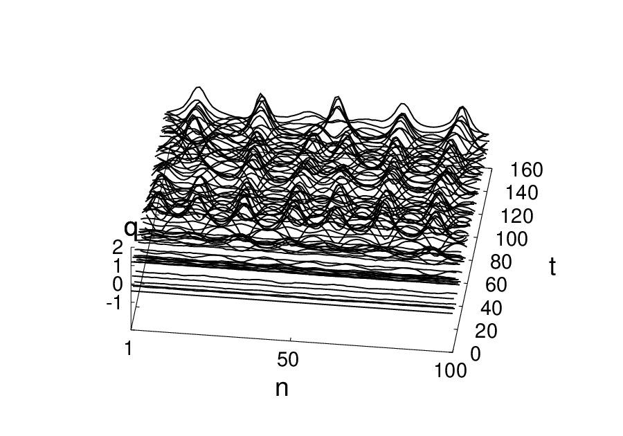

showing the spatio-temporal evolution of the amplitudes for couplings and . The Langevin equations were numerically integrated using a two-step Heun stochastic solver. In all our simulations the initial chain configuration is represented by and with the homogeneous solution (plane wave) given in (7). We note the formation of a LM of certain wave length arising from the homogeneous state after a short time span (after ) and we note that the period duration for oscillations near the bottom of the potential is around .
Regarding the energy relation within the stationary flat state (where each unit contains the same amount of initial energy) we monitored the temporal evolution of the energy of one unit
| (11) |
and the corresponding field energy
| (12) |
without coupling the chain to the heat bath for a force amplitude . In this stationary case the field energy performs small-amplitude oscillations around a mean value of , while the mean of the energy of one unit is (not shown). Thus the gain of energy, determined by the ratio , amounts to a remarkable high value of . To retain this relation upon lowering (increasing) the damping a lower (higher) driving strength is necessary while the ”jump” resonance frequency attains a lower (higher) value according to Eq. (6).
The stochastic term provides perturbations of all wave numbers and a pattern emerges from the homogeneous flat state. That is, due to the effect of parametric resonance perturbations provided by the thermal noise grow and induce a LM consisting of several humps. The fastest growing perturbations are those associated with the critical wave number (see also [34]). Each of these humps resembles the hairpin shape of the transition state as the critical escape configuration possessing an energy through which the coupled units have to pass in order to cross the barrier [30]. The robustness of the LMs is remarkable: a LM is sustained despite continuously impacting thermal noise of strengths up to values . Moreover, the formed pattern maintain their distinct wave length (see Fig. 3).
We note that upon increasing the noise strength the growth rate of the humps becomes enhanced, being reflected in the statistics of the barrier crossing of the chain in the presence of weak ac-driving. The amplitude and frequency of the latter are chosen such that the dynamics exhibits parametric resonance. The dependence of the mean escape time of the chain on the injected average energy , with (measured in units of the barrier energy ) is displayed in Fig. 4. The thermal energy , supplied non-coherently by the heat bath, is varied within the range .

The average of the escape times was performed over realizations of the thermal noise. In this context the random escape time of a unit is defined as the time instant when the unit passes through the value far beyond the potential barrier. Thus, no likely recrossing back into the potential valley can occur [29, 30]. The escape time of the chain is then determined by the average of the escape times of its units. We notice that the underlying irregular dynamics serves for self-averaging and thus the choice of the phase of the coherent, external forcing, , does not affect the mean escape time. In the forced as well as unforced case there occurs a rather rapid decay of with growing at low temperatures. This effect weakens gradually upon further increasing . Most strikingly, for the forced system the escape times become drastically shortened in comparison with the unforced case with . Moreover, for the forced system escape takes place also at very low temperatures for which in the undriven case not even the escape of a single unit has been observed during the simulation time (taken here as ) implying a giant enhancement of the rate of escape as compared to the purely thermal noise driven rate.
Upon exploring the optimal escape route we investigated the influence of the coupling strength on the average escape time. Our numerical findings are summarized in Fig. 5.

The mean escape time exhibits a resonance structure, viz. there exists an optimal coupling strength () for which the escape assumes a minimum. Upon lowering we notice a drastic rise of the escape time while for the graph exhibits only a moderately growing slope with growing coupling strength . We emphasize the collective nature of this resonance effect which here occurs for finite interaction strength . In the limit the mean escape time of noninteracting, individual particles assumes for this parameter set an extreme large value, implying a vanishingly small escape rate.
To explain the occurrence of the resonance structure in Fig. 5 we recall that the wave length, , of the arising LMs on the lattice is determined by the critical wave number (cf. Fig. 2). The number of humps contained in a LM, , can be attributed to as: . The number of humps (besides their height and width) regulates how the mean energy injected via the coherent external field and the incoherent thermal noise is shared among them. Supposing that the whole lattice can be divided into an array of segments, where each of them supports a single localized hump, the energy of one segment is given by . Appropriate conditions for successful escape are provided when the energy contained in each segment, , is close to the activation energy, of the critical escape configuration [30]. The efficiency of energy localization is then determined by the ratio
| (13) |

The activation energy as a function of the coupling strength satisfies (we recall that we use a dimensionless formulation) the relation [30]. Keeping the injected energy fixed and given value of we obtain . In the inset of Fig. 5 the ratio is plotted as a function of the coupling strength . The plot indeed exhibits a maximum at , which confirms the finding of the resonance found for the mean escape time versus coupling strength as depicted in Fig. 5. Concerning the critical localized mode through which a lattice state has to pass through in order to escape over the potential barrier we remark that for comparatively low coupling strengths () the effect of discreteness in the lattice system is still such pronounced that this critical localized mode is indeed represented by a thin hairpin-shaped configuration involving effectively one lattice unit of large amplitude to either side of which the amplitude pattern decays extremely rapidly (for more details see [30]).
Next we study the role of the angular driving frequency of the external modulation field, see in Fig. 6. The escape time as a function of the angular frequency likewise exhibits a resonance structure and there exists an optimal frequency for which the average escape time assumes a minimum. This is reminiscent of the phenomenon of resonant activation found for the thermally activated escape of noninteracting particles surmounting oscillating barriers [23, 24, 25, 26, 27]. In our case of a nonlinear chain composed of coupled units, however, this ’resonant activation’ within a frequency window nicely correlates with the systems’ gain of energy that is coherently supplied by the applied ac-field in this very same frequency interval (note the corresponding frequency window in the nonlinear frequency response graph associated with large amplitudes in Fig. 1). Therefore, tuning the frequency at a fixed interaction strength allows to optimize further the mean escape time. The minimal escape scenario thus requires an optimal tuning both in coupling strength and ac-driving frequency .
In summary, we have presented a drastic speed-up mechanism of the thermal noise driven barrier crossing of a coupled damped nonlinear oscillator chain under the impact of a weak external ac-field. With appropriate parameter values of the latter and in the presence of thermal noise an instability mechanism is initiated due to which LMs arise from stationary flat state solutions in the lattice dynamics. Humps of the LMs are rapidly driven through the transition state thus accelerating the escape over the situation with purely thermally assisted escape. Interestingly, the LMs are sustained up to fairly high noise levels corresponding to .
The findings of our study can be applied for the control of the rate of barrier crossing of oscillator chains. With such chains providing the archetype model for nonlinear collective transport of matter, charge and energy in abundant low-dimensional systems in physics, biology and chemistry this speed-up scenario of thermally driven collective escape over potential barriers might well be put to constructive use in a variety of potential applications.
Acknowledgments
This research has been supported by SFB-555 (L. Sch.-G) and, as well, by the joint Volkswagen Foundation projects I/80424 (P. H.) and I/80425 (L. Sch.-G).
References
- [1] Hänggi P., Talkner P. and Borkovec M., Rev. Mod. Phys. 62 (1990) 251.
- [2] Hänggi P., J. Stat. Phys. 42 (1986) 105; J. Stat. Phys. 44 (1986) 1003 .
- [3] Langer J. S., Ann. Phys. (N.Y.) 54 (1969) 258 .
- [4] Hänggi P., Marchesoni F., and Sodano P., Phys. Rev. Lett. 60 (1988) 2563; Hänggi P. and Marchesoni F., Phys. Rev. Lett. 77 (1996) 787.
- [5] Marchesoni F., Gammaitoni L., and Bulsara A.R., Phys. Rev. Lett. 76 (1996) 2609.
- [6] Sung W. and Park P. J., Phys. Rev. Lett.77 (1996) 783.
- [7] Park P. J. and Sung W., Phys. Rev. E 57 (1998) 730 ; J. Chem. Phys. 108 (1998) 3013 ; ibid 111 (1999) 5259.
- [8] Sebastian K. L. and Paul A. K. R., Phys. Rev. E 62 (2000) 927.
- [9] Lee S. and Sung W., Phys. Rev. E 63 (2001) 021115; Lee K. and Sung W., Phys. Rev. E 64 (2001) 041801.
- [10] Kraikivsky P., Lipowsky R., and Kiefeld J., Europhys. Lett. 66 (2004) 763 .
- [11] Dowtown M. T., Zuckermann M. J., Craig E. M., Plischke M., and Linke H., Phys. Rev. E 73 (2006) 011909.
- [12] Hänggi P., Marchesoni F., and Nori F., Ann. Physik (Leizig) 14 (2005) 51.
- [13] Astumian R. D. and Hänggi P., Physics Today 55 (11) (2002) 33; Reimann P. and Hänggi P., Appl. Phys. A 75 (2002) 169.
- [14] Cattuto C. and Marchesoni F., Europhys. Lett. 62 (2003) 363.
- [15] Marin J.L. and Aubry S., Nonlinearity 9 (1994) 1501.
- [16] Hennig D., Phys. Rev. E 59 (1998) 1637.
- [17] Vanossi A., Rasmussen K.Ø., Bishop A.R., Malomed B.A., and Bortolani V., Phys. Rev. E 62 (2000) 7353.
- [18] Marin J.L., Falo F., Martinez P.J., and Floria L.M., Phys. Rev. E 63 (2001) 066603.
- [19] Maniadis P. and Flach S., Europhys. Lett. 74 (2006) 452.
- [20] Nosé S., J. Chem. Phys. 81 (1984) 511.
- [21] Peyrard M., Physica D 119 (1998) 84; Dauxois T., Peyrard M., and Bishop A.R., Phys. Rev. E 47 (1993) 684.
- [22] Tsironis G.P. and Aubry S., Phys. Rev. Lett. 77 (1996) 5225.
- [23] Doering C. and Gadoua J.C., Phys. Rev. Lett. 69 (1992) 2318.
- [24] Lehmann J., Reimann P., and Hänggi P., Phys. Rev. Lett 84 (1999) 1639; Phys. Rev. E 62 (2000) 6282.
- [25] Mantegna R. N. and Spagnolo B., Phys. Rev. Lett. 84 (2000) 3025.
- [26] Reimann P. and Hänggi P., Surmounting fluctuating barriers: Basic concepts and exact results; in: Stochastic Dynamics, eds. L. Schimansky-Geier and Th. Pöschel, Lecture Notes in Physics, 484 (1997) 127.
- [27] Pechukas P. and Hänggi P., Phys. Rev. Lett. 73 (2004) 2772.
- [28] Sustanski A.L. and Primak K.I., Phys. Rev. Lett. 75 (1995) 3029; Kivshar Yu. S. and Sanchez A., Phys. Rev. Lett. 77 (1996) 582.
- [29] Hennig D., Schimansky-Geier L., and Hänggi P., Europhys. Lett. 78 (2007) 20002.
- [30] Hennig D., Fugmann S., Schimansky-Geier L., and Hänggi P. Phys. Rev. E 76 (2007) 041110.
- [31] Kivshar Yu. S., Phys. Rev. E 48 (1993) 4132; Daumont I., Dauxois T., and Peyrard M., Nonlinearity 10 (1997) 617.
- [32] V.I. Arnold, Mathematical Methods of Classical Mechanis (Springer, New York, 1997).
- [33] L.D. Landau and E.M. Lifshitz Course of Theoretical Physics: Mechanics (Akademie-Verlag, Berlin, 1987).
- [34] Kolomeisky E.B., Curcic T, and Straley J.P., Phys. Rev. Lett. 75 (1995) 1775.