跳到论文正文
W Papers独立论文阅读器 arXiv:0807.4576 论文正文 计算阅读时间 · 0%
引用这篇论文根据当前论文元数据生成,正式投稿前建议核对。


License: arXiv.org perpetual non-exclusive license
arXiv:0807.4576v1 [quant-ph] 29 Jul 2008

Designing the unambiguous discriminator from the one-photon interferometer

Xiaohua Wu Address: Department of Physics, Sichuan University, Chengdu 610064, China.    Yu Shaolan Address: Department of Physics, Sichuan University, Chengdu 610064, China.    Zhou Tao Address: Department of Physics, Sichuan University, Chengdu 610064, China.
Abstract

The quantum states filtering, whose general theorem was given by Bergou et al. (Phys.Rev.A 71, 042314(2005)), should find it’s important applications in present scheme, where we are trying to show that the problem of quantum states unambiguous discrimination may be solved by applying the argument of filtering. Let’s use the quantum filtering, as an example, to show the basic idea of present scheme. Suppose there are N linearly independent states, if we are able to find a (N+1)-dimensional unitary transformation, R⁡(ω)R(\omega) ( with ω\omega is an adjustable variable(s)), which will be performed on each |Ψ>|\Psi> in the way like: R⁡(ω)|Ψ1>=d11​(ω)|D1>+f1​(ω)|F>R(\omega)|\Psi_{1}>=d_{11}(\omega)|D_{1}>+f_{1}(\omega)|F>, R⁡(ω)|Ψk>=∑l=2Ndk​l​(ω)|Dl>+fk​(ω)|F>R(\omega)|\Psi_{k}>=\sum_{l=2}^{N}d_{kl}(\omega)|D_{l}>+f_{k}(\omega)|F>, then, according to the definition of the operators for filtering, there should be: E1​(ω)=R−1​(ω)|D1><D1|R⁡(ω)E_{1}(\omega)=R^{-1}(\omega)|D_{1}><D_{1}|R(\omega), E2​(ω)=∑k=2NR−1​(ω)|Dk><Dk|R⁡(ω)E_{2}(\omega)=\sum_{k=2}^{N}R^{-1}(\omega)|D_{k}><D_{k}|R(\omega) and E0​(ω)=R−1​(ω)|F><F|R⁡(ω)E_{0}(\omega)=R^{-1}(\omega)|F><F|R(\omega). With this this {Em​(ω)}\{E_{m}(\omega)\} in hands, we could find the optimal operators which lets the function F⁡(ω)=∑j=1ηj​<Ψj|E0​(ω)|Ψj>F(\omega)=\sum_{j=1}\eta_{j}<\Psi_{j}|E_{0}(\omega)|\Psi_{j}>, with ηj\eta_{j} to be the a​𝑝𝑟𝑖𝑜𝑟𝑖{\sl a~priori} probability of |Ψj>|\Psi_{j}>, have it’s minimum value. For the system with N=3, there are three types of operations: (a) E1a|Ψ2>=E1a|Ψ3>=0E^{a}_{1}|\Psi_{2}>=E^{a}_{1}|\Psi_{3}>=0, E2a|Ψ1>=0E^{a}_{2}|\Psi_{1}>=0 and E0aE^{a}_{0} corresponds to fail; (b) Eib|Ψj>=0E_{i}^{b}|\Psi_{j}>=0 if i≠ji\neq j for i=1,2,3, and E0bE^{b}_{0} for failure; and (c) E1c|Ψ2>=E1c|Ψ3>=0,E^{c}_{1}|\Psi_{2}>=E^{c}_{1}|\Psi_{3}>=0, E2c|Ψ1>=E1c|Ψ3>=0,E^{c}_{2}|\Psi_{1}>=E^{c}_{1}|\Psi_{3}>=0, while E0c=I −∑k=12Ek.E^{c}_{0}=\textbf{I }-\sum_{k=1}^{2}E_{k}. We shall show that all these three types of operators, which may be performed on a N=3 systems, can be get by applying argument of filtering: the case a is in fact the filtering with N=3, case b can be viewed as successive filtering and the case c can also be solved by an argument of filtering in subspace. It can be shown that each case, which belongs to the above three, can be solved by reducing it to the problem of filtering. An important case of N=4 system, has also been discussed.

pacs
03.67.Lx

I introduction

As a very recent development, the possibility of unambiguous discrimination between unknown quantum states can be potentially useful for many applications in quantum computing and quantum communications. The problem of unambiguous discriminating pure states, which are successfully identified with nonunit probability but witout error, was originally formulated and analyzed by Ivanovic, Dicks and Peres [1-3] in 1987. Later, Jeager and Shimony solved the question of unambiguous discrimination of two known pure states with arbitrary a​p​r​i​o​r​i{a~priori} probability. Shortly after this result, Chefles proved that only linearly independent pure states can be unambiguously discriminated [5]. The problem of discrimination among three nonorthogonal states was first considered by Peres and Terno [6], and the same question has also been discussed by Duan and Guo[7] and Sun 𝑒𝑡​𝑎𝑙.{\sl et~al.} [8]. Chefles and Barnett also provided the optimal failure probability and it’s corresponding optimal measurement for a n symmetric states [9], and an experimental set for discriminating four linearly independent nonorthogonal symmetric states was given by Jiménez 𝑒𝑡​𝑎𝑙.{\sl et~al.} [10]. A new strategy for optimal unambiguous discrimination of quantum states was also offered by Jafarizadeh 𝑒𝑡​𝑎𝑙.{\sl et~al.} [11].

Unambiguous discrimination involving mixed state or a set of pure states, became an object of research recently. Several necessary and sufficient conditions for the optimum measurement have been given by Zhang 𝑒𝑡​𝑎𝑙.{\sl et~al.} [12] and Eldar 𝑒𝑡​𝑎𝑙.{\sl et~al.} [13]. Reduction theorems, which can simplify the discrimination theorem, have been developed by Raynal 𝑒𝑡​𝑎𝑙.{\sl et~al.} [14-15]. Low bounds for the failure and the conditions for saturating the boumds, have also been studied [16-20]. There are only a few special cases have analytical solution for the quantum measurement, for examples, the quantum state filtering [21-23], two mixtures with orthogonal or one-dimensional kernels [14-15], two mixtures in The Jordan basis [24] and other cases [26-30).

In present work, we shall present a new scheme to solve the problem of quantum state unambiguous discrimination. Let’s use the quantum state filtering originated from [21-23], as an example, to show the basic idea of present scheme. Suppose there are N linearly independent states, the task of the quantum state filtering can be viewed as to find a set of operators {Em}\{E_{m}\}, whose elements are defined by : E2|Ψ1>=0E_{2}|\Psi_{1}>=0, E1|Ψk>=0E_{1}|\Psi_{k}>=0 with 2≤k≤N2\leq k\leq N, and E0E_{0} corresponds to fail. If we are able to find a (N+1)-dimensional unitary transformation, R⁡(ω)R(\omega) with ω\omega is an adjustable variable(s), which will be performed on each |Ψ>|\Psi> in the way like: R⁡(ω)|Ψ1>=d11​(ω)|D1>+f1​(ω)|F>R(\omega)|\Psi_{1}>=d_{11}(\omega)|D_{1}>+f_{1}(\omega)|F>, R⁡(ω)|Ψk>=∑l=2Ndk​l​(ω)|Dl>+fk​(ω)|F>R(\omega)|\Psi_{k}>=\sum_{l=2}^{N}d_{kl}(\omega)|D_{l}>+f_{k}(\omega)|F>, then, according to the definition of the operators, there should be: E1​(ω)=R−1​(ω)|D1><D1|R⁡(ω)E_{1}(\omega)=R^{-1}(\omega)|D_{1}><D_{1}|R(\omega), E2​(ω)=∑k=2NR−1​(ω)|Dk><Dk|R⁡(ω)E_{2}(\omega)=\sum_{k=2}^{N}R^{-1}(\omega)|D_{k}><D_{k}|R(\omega) and E0​(ω)=R−1​(ω)|F><F|R⁡(ω)E_{0}(\omega)=R^{-1}(\omega)|F><F|R(\omega), With this {Em​(ω)}\{E_{m}(\omega)\} in hands, we could find the optimal operators which lets the function F⁡(ω)=∑j=1ηj​<Ψj|E0​(ω)|Ψj>F(\omega)=\sum_{j=1}\eta_{j}<\Psi_{j}|E_{0}(\omega)|\Psi_{j}>, with ηj\eta_{j} to be the a​𝑝𝑟𝑖𝑜𝑟𝑖{\sl a~priori} probability of |Ψj>|\Psi_{j}>, have it’s minimal value.

For the system with N=3, there are three types of operations: (a) E1a|Ψ2>=E1a|Ψ3>=0E^{a}_{1}|\Psi_{2}>=E^{a}_{1}|\Psi_{3}>=0, E2a|Ψ1>=0E^{a}_{2}|\Psi_{1}>=0 and E0aE^{a}_{0} corresponds to fail; (b) Eib|Ψj>=0E_{i}^{b}|\Psi_{j}>=0 if i≠ji\neq j for i=1,2,3, and E0bE^{b}_{0} for failure; and (c) E1c|Ψ2>=E1c|Ψ3>=0,E^{c}_{1}|\Psi_{2}>=E^{c}_{1}|\Psi_{3}>=0, E2c|Ψ1>=E1c|Ψ3>=0,E^{c}_{2}|\Psi_{1}>=E^{c}_{1}|\Psi_{3}>=0, while E0c=I −∑k=12Ek.E^{c}_{0}=\textbf{I }-\sum_{k=1}^{2}E_{k}. We shall show that all these three types of operators, which may be performed on a N=3 systems, can be get by applying argument of filtering: the case a is in fact the filtering with N=3, case b can be viewed as successive filtering and the case c can also be solved by an argument of filtering in subspace. It looks as if each case, which belongs to the above three, can be solved by reducing it to the problem of filtering. An important case of N=4 system, has also been discussed.

Our present paper is organized as follows. Section II is a preliminary section in which we introduce the so-called double-triangle representation. In section III, we shall give a different way of solving the question of quantum states filtering. A concept of filtering in subspace will be introduced in Sec.IV. Two examples, discriminating three pure states and discriminating two mixtures for N=4, will be discussed in Section V and VI, respectively. In Sec.VII, we conclude the paper with a short summary.
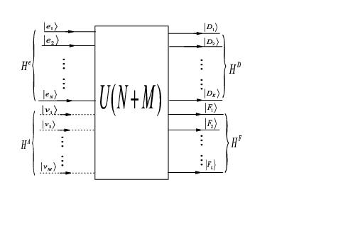
Refer to caption
Figure 1: An optical setting to realize the POVMs in an enlarged Hilbert space

II double triangle representation

II.1 preliminary

Considering a quantum system prepared in one of N pure quantum states |Ψj>|\Psi_{j}>, where j=1, 2,…, N, if the states are non-orthogonal, no quantum operations can deterministically discriminate them. It is, however, possible to device a strategy reveal the state with zero error probability under the condition that these states are linearly independent [5]. Employing the Kraus representation of quantum operations [31], each of the possible distinguishable outcomes of an operation is associated with linear transformation operators A^m\hat{A}_{m},

∑m=oNA^m†​A^m=I,\sum_{m=o}^{N}\hat{A}^{\dagger}_{m}\hat{A}_{m}=\textbf{I}, (2.1)

with A^0\hat{A}_{0} leads to failure while A^j\hat{A}_{j} corresponds to the discrimination of |Ψj>|\Psi_{j}>. By introducing the 𝑟𝑒𝑐𝑖𝑝𝑟𝑜𝑐𝑎𝑙​𝑠𝑡𝑎𝑡𝑒𝑠{\sl reciprocal~states} |Ψ⊥j>|\Psi^{\bot}_{j}>, which is defined as that which lies in ℋ\mathcal{H}, the N-dimensional Hilbert space for the N linearly independent states |Ψj>|\Psi_{j}>, and is orthogonal to all Ψj′\Psi_{j^{\prime}} for j≠j′j\neq j^{\prime}, Chefles found that [5]

A^j=pj1/2<Ψj⊥|Ψj>|ej><Ψ⊥j|,\hat{A}_{j}=\frac{p^{1/2}_{j}}{<\Psi^{\bot}_{j}|\Psi_{j}>}|e_{j}><\Psi^{\bot}_{j}|, (2.2)

where |ej>|e_{j}> form an orthonormal basis for ℋ\mathcal{H} while PjP_{j} is the conditional probability, given that the system was prepared in the state |Ψj>|\Psi_{j}>, that this state will be identified,

<ψj|A^j′†​A^j′|Ψj>=Pj​δj​j′.<\psi_{j}|\hat{A}^{\dagger}_{j^{\prime}}\hat{A}_{j^{\prime}}|\Psi_{j}>=P_{j}\delta_{jj^{\prime}}. (2.3)

In the terms of positive operator valued measures (POVMs) [31], the measurement can be expressed by defining the positive Hermitian operators

Ej\displaystyle E_{j} =\displaystyle= A^†jA^j=pj|<ψj⊥|ψj>|2|Ψj⊥><Ψj⊥|,\displaystyle\hat{A}^{\dagger}_{j}\hat{A}_{j}=\frac{p_{j}}{|<\psi^{\bot}_{j}|\psi_{j}>|^{2}}|\Psi_{j}^{\bot}><\Psi_{j}^{\bot}|,
E0\displaystyle E_{0} =\displaystyle= A^0+​A^0,\displaystyle\hat{A}^{+}_{0}\hat{A}_{0}, (2.4)

with E0+∑j=1NEj=IE_{0}+\sum_{j=1}^{N}E_{j}=\textbf{I}, and it has been shown that the optimum measurement corresponds to the maximum eigenvalue of value of ED=∑j=1NEjE_{D}=\sum_{j=1}^{N}E_{j} being equal to 1 [5].

Let G≡{|Ψj>}G\equiv\{|\Psi_{j}>\} for j=1, 2,…, N, the POVMs given above can viewed as one type of operations on G. There may be other types of operations on the same G, for example, if there are two known groups of states, G1≡{|Ψk>}G_{1}\equiv\{|\Psi_{k}>\} for k=1, 2, …, K, and G2≡{|Ψl>}G_{2}\equiv\{|\Psi_{l}>\} for l= L, L+1, …, N, G1G_{1} and G2G_{2} may have common elements if L≤KL\leq K, we could also define a new set of POVMs {Ei,E0}\{E_{i},E_{0}\} for i=1, 2, EiE_{i} can unambiguously tell whether a state |Ψ?>∈G|\Psi_{?}>\in G belongs to GiG_{i} or not. Now, one may ask the question: could this {Em}\{E_{m}\} also be expressed in terms of |Ψ⊥i><Ψ⊥j||\Psi^{\bot}_{i}><\Psi^{\bot}_{j}|? We shall give an answer to this question. According to the Neumark’s theorem [32]: if each EmE_{m} is an one dimensional positive operator, {Em}\{E_{m}\} can always be realized by extending the Hilbert space to a larger space and performing orthogonal measurement in the larger space, while, as we shall shown, we are able to realize the discrimination of the quantum states just according to the definition of the operators, this fact makes it possible to read {Em}\{E_{m}\} from their corresponding projective operators in the enlarged space. We shall show how this basic idea works via the aid of Fig.1: the total space is defined to be H=He+HAH=H^{e}+H^{A} with {|ei>,|vj>}\{|e_{i}>,|v_{j}>\}, i=1, 2, …, N, and j=1, 2, …, M, for it’s ”in-space” while {|Dk>,|Fl>}\{|D_{k}>,|F_{l}>\} for it’s ”out-space” with 1≤k≤K1\leq k\leq K, 1≤l≤L1\leq l\leq L, and N+M=K+L. HeH^{e} is the Hilbert space where the states are defined:

|Ψi>=∑j=1Nci​j|ej>,|\Psi_{i}>=\sum_{j=1}^{N}c_{ij}|e_{j}>, (2.5)

HAH^{A} is the subspace for ancillas, U(N+M) will couple this two subspace together. Let’s use ω\omega to denote the adjustable parameter(s) in the unitary transformation, we can define |ψ>o​u​t=U(ω)|Ψ>|\psi>^{out}=U(\omega)|\Psi> and express it in the ”out-space”

|ψj>o​u​t=∑k=1Kdj​k(ω)|Dk>+∑l=1Lfj​l(ω)|Fl>,|\psi_{j}>^{out}=\sum_{k=1}^{K}d_{jk}(\omega)|D_{k}>+\sum_{l=1}^{L}f_{jl}(\omega)|F_{l}>, (2.6)

with the normalization constraint ∑k=1K|dj​k|2+∑l=1L|fj​l|2=1.\sum_{k=1}^{K}|d_{jk}|^{2}+\sum_{l=1}^{L}|f_{jl}|^{2}=1. If we want to unambiguously discriminate all Ψj\Psi_{j} in G, we should find the general U⁡(ω)U(\omega) which gives

|ψj>o​u​t=dj​j(ω)|Dj>+∑l=1Lfj​l(ω)|Fl>,|\psi_{j}>^{out}=d_{jj}(\omega)|D_{j}>+\sum_{l=1}^{L}f_{jl}(\omega)|F_{l}>, (2.7)

then, |Dj><Dj||D_{j}><D_{j}| and ∑l=1L|Fl><Fl|\sum_{l=1}^{L}|F_{l}><F_{l}| should be the projective operator corresponds to EjE_{j} and E0E_{0}, respectively. With the U⁡(ω)U(\omega), we could write , for example, |Dj>|D_{j}> in the ”in-space” as |Dj>i​n=U−1|Dj>=|Dj>e+|Dj>A|D_{j}>^{in}=U^{-1}|D_{j}>=|D_{j}>^{e}+|D_{j}>^{A} with |Dj>e|D_{j}>^{e} and |Dj>A|D_{j}>^{A} are two non-normalized vectors which lies in HeH^{e} and HAH^{A}, respectively. There should be

Ej(ω)=|Dj>e<Dj|,E0(ω)=∑l=1L|Fl>e<Fl|,E_{j}(\omega)=|D_{j}>^{e}<D_{j}|,~~~E_{0}(\omega)=\sum_{l=1}^{L}|F_{l}>^{e}<F_{l}|, (2.8)

and E0​(ω)+∑j=1NEj​(ω)=IeE_{0}(\omega)+\sum_{j=1}^{N}E_{j}(\omega)=\textbf{I}^{e}. With these operators in hands, we could get both the optimal operators and the maximum values for discriminating |Ψj>|\Psi_{j}>. When the projective operators are expressed in the ”in-space”, there are written formally in terms of |ei><ej||e_{i}><e_{j}|. If we could define {|ej>}\{|e_{j}>\} by {|Ψj⊥>}\{|\Psi_{j}^{\bot}>\} at the beginning, then we shall be able to complete the task of expressing EmE_{m} in terms of |Ψi⊥><Ψj⊥||\Psi_{i}^{\bot}><\Psi_{j}^{\bot}|. The argument above can also be generalized to other cases with different operations on G.

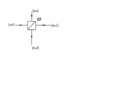
In present works, we always adopt the proposals originated from the works by Sun 𝑒𝑡​𝑎𝑙.{\sl et~al.} [8]: (a) any pure state can be realized by a single-photon state and (b), according to Reck’s theorem [34], any unitary transformation matrix can also be realized by an optical network consisting of beam-splitters, phase-shifters, 𝑒𝑡𝑐.{\sl etc.}, all these optical elements should construct an one-photon interferometer (OPI). The device in Fig.2 is a typical four-port beam splitter which is used to realize a two-dimensional unitary transformation U2​(ω)U_{2}(\omega):

(−sin⁡ωcos⁡ωcos⁡ωsin⁡ω)​(|ω,r>|ω,d>)=(|ω,l>|ω,u>).\left(\begin{array}[]{cc}-\sin\omega&\cos\omega\\ \cos\omega&\sin\omega\\ \end{array}\right)\left(\begin{array}[]{c}|\omega,r>\\ |\omega,d>\\ \end{array}\right)=\left(\begin{array}[]{c}|\omega,l>\\ |\omega,u>\\ \end{array}\right). (2.9)

A property of this beam-splitter, which is frequently applied in present works, should be noted: suppose there is an input

|ϕ>=cw,l|ω,l>+cw,u|ω,u>,|\phi>=c_{w,l}|\omega,l>+c_{w,u}|\omega,u>, (2.10)

where cw,lc_{w,l} and cw,uc_{w,u} are real parameters for simplicity, after performing the U2​(ω)U_{2}(\omega), the output should be

|ϕ′>=U2(ω)|ϕ>=cw,r|ω,r>+cw,d|ω,d>|\phi^{\prime}>=U_{2}(\omega)|\phi>=c_{w,r}|\omega,r>+c_{w,d}|\omega,d> (2.11)

with the coefficients satisfy:

cω,r\displaystyle c_{\omega,r} =\displaystyle= −cω,l​sin⁡ω+cω,u​cos⁡ω,\displaystyle-c_{\omega,l}\sin\omega+c_{\omega,u}\cos\omega, (2.12)
cω,d\displaystyle c_{\omega,d} =\displaystyle= cω,l​cos⁡ω+cω,u​sin⁡ω,\displaystyle\ c_{\omega,l}\cos\omega+c_{\omega,u}\sin\omega, (2.13)

if we choose

sin⁡ω=cω,ucω,l2+cω,u2,cos⁡ω=cω,rcω,l2+cω,u2,\sin\omega=\frac{c_{\omega,u}}{c_{\omega,l}^{2}+c_{\omega,u}^{2}},~~\cos\omega=\frac{c_{\omega,r}}{c_{\omega,l}^{2}+c_{\omega,u}^{2}}, (2.14)

then |ϕ′>=(cω,l2+cω,u2)|ω,d>|\phi^{\prime}>=(c_{\omega,l}^{2}+c_{\omega,u}^{2})|\omega,d> while it’s output along |ω,r>|\omega,r> is zero.

Refer to caption
Figure 2: A four-port beam-splitter used to realize a two-dimensional unitary transformation

II.2 which parameters are known?

In present work, we shall deal with the case that all the states in G are linearly independent and their overlaps are also known.

Definition  2.1:  a N-dimensional matrix O(N) is defined by it’s matrix elements

oi​j=<Ψi|Ψj>,o_{ij}=<\Psi_{i}|\Psi_{j}>, (2.15)

with constraint that |Oi​j|<1|O_{ij}|<1 holds for i≠ji\neq j.

Certainly, O(N) is Hermitian. Using O*(N) and O~​(N)\tilde{O}(N) for it’s conjugate matrix and transposed matrix, respectively, there should be Oi​j∗=O~i​j=oj​iO^{*}_{ij}=\tilde{O}_{ij}=o_{ji}.

Definition  2.2: A(N) is used to denote the adjoint matrix of O(N), Ai​j=ai​jA_{ij}=a_{ij}, the inverse of O should be

O−1​(N)=A⁡(N)det(O),O^{-1}(N)=\frac{A(N)}{\det(O)}, (2.16)

where det(O)\det(O) denotes the determinate of O(N).

Definition  2.3:  tjt_{j} is used to denote

tj=<ψj⊥|Ψj>.t_{j}=<\psi^{\bot}_{j}|\Psi_{j}>. (2.17)

From the definition of the reciprocal states, if |Ψj>|\Psi_{j}> is a the reciprocal state of |Ψj>|\Psi_{j}>, then exp⁡{i​ϕj}|Ψj>\exp\{i\phi_{j}\}|\Psi_{j}> is also a reciprocal state of |Ψj>|\Psi_{j}>. We can always let tj=<ψj⊥|Ψj>=<ψj|Ψj⊥>t_{j}=<\psi^{\bot}_{j}|\Psi_{j}>=<\psi_{j}|\Psi_{j}^{\bot}> by choosing a suitable set of {ϕj}\{\phi_{j}\}. Defining

|Ψj∥>=11−tj2(|Ψj>−tj|Ψ⊥>),|\Psi^{\|}_{j}>=\frac{1}{\sqrt{1-t_{j}^{2}}}(|\Psi_{j}>-t_{j}|\Psi^{\bot}>), (2.18)

one may verified that |Ψj⊥>|\Psi_{j}^{\bot}> and |Ψ∥j>|\Psi^{\|}_{j}> form an orthonormal basis for |Ψj>|\Psi_{j}> and

|Ψj>=1−tj2|Ψ∥j>+tj|Ψj⊥>,|\Psi_{j}>=\sqrt{1-t_{j}^{2}}|\Psi^{\|}_{j}>+t_{j}|\Psi_{j}^{\bot}>, (2.19)

it should be emphasized here that, either |Ψj⊥>|\Psi_{j}^{\bot}> or |Ψ∥j>|\Psi^{\|}_{j}>, is defined from all the states in G:

𝑇ℎ𝑒𝑜𝑟𝑒𝑚​2.1:<Ψj⊥|Ψk>=tj​δj​k.{\sl Theorem~~2.1}:~~~<\Psi_{j}^{\bot}|\Psi_{k}>=t_{j}\delta_{jk}. (2.20)

With the tjt_{j} and O(N) defined above, we may introduced another transformation matrix:

Theorem   2.2:   denoting (δi​j)=I(\delta_{ij})=\textbf{I}, and defining

R⁡(N)=O~​(N)​(1tj​δi​j),R(N)=\tilde{O}(N)(\frac{1}{t_{j}}\delta_{ij}), (2.21)

there should be

R⁡(N)|Ψ⊥>=|Ψ>.R(N)|\Psi^{\bot}>=|\Psi>. (2.22)

Proof: formally, we can write |Ψj>|\Psi_{j}> as a linear combination of {|Ψk⊥>}\{|\Psi^{\bot}_{k}>\} in the way like |Ψj>=∑k=1Nhj​k|Ψ⊥k>|\Psi_{j}>=\sum_{k=1}^{N}h_{jk}|\Psi^{\bot}_{k}>, there should be oi​j=<Ψi|Ψj>=∑k=1Nhj​k​<Ψi|Ψk⊥>=hj​i​tio_{ij}=<\Psi_{i}|\Psi_{j}>=\sum_{k=1}^{N}h_{jk}<\Psi_{i}|\Psi^{\bot}_{k}>=h_{ji}t_{i}, which gives |Ψj>=∑k=1Nok​jtk|Ψ⊥k>|\Psi_{j}>=\sum_{k=1}^{N}\frac{o_{kj}}{t_{k}}|\Psi^{\bot}_{k}>. Let N=3, as an example, we have

|Ψ1⊥><Ψ1|Ψ1⊥>+o21|Ψ2⊥><Ψ2|Ψ2⊥>+o31|Ψ3⊥><Ψ3|Ψ3⊥>\displaystyle\frac{|\Psi_{1}^{\bot}>}{<\Psi_{1}|\Psi_{1}^{\bot}>}+\frac{o_{21}|\Psi_{2}^{\bot}>}{<\Psi_{2}|\Psi_{2}^{\bot}>}+\frac{o_{31}|\Psi_{3}^{\bot}>}{<\Psi_{3}|\Psi_{3}^{\bot}>} =\displaystyle= |Ψ1>\displaystyle|\Psi_{1}>
o12|Ψ1⊥><Ψ1|Ψ1⊥>+|Ψ2⊥><Ψ2|Ψ2⊥>+o32|Ψ3⊥><Ψ3|Ψ3⊥>\displaystyle\frac{o_{12}|\Psi_{1}^{\bot}>}{<\Psi_{1}|\Psi_{1}^{\bot}>}+\frac{|\Psi_{2}^{\bot}>}{<\Psi_{2}|\Psi_{2}^{\bot}>}+\frac{o_{32}|\Psi_{3}^{\bot}>}{<\Psi_{3}|\Psi_{3}^{\bot}>} =\displaystyle= |Ψ2>\displaystyle|\Psi_{2}>
o13|Ψ1⊥><Ψ1|Ψ1⊥>+o23|Ψ2⊥><Ψ2|Ψ2⊥>+|Ψ3⊥><Ψ3|Ψ3⊥>\displaystyle\frac{o_{13}|\Psi_{1}^{\bot}>}{<\Psi_{1}|\Psi_{1}^{\bot}>}+\frac{o_{23}|\Psi_{2}^{\bot}>}{<\Psi_{2}|\Psi_{2}^{\bot}>}+\frac{|\Psi_{3}^{\bot}>}{<\Psi_{3}|\Psi_{3}^{\bot}>} =\displaystyle= |Ψ3>\displaystyle|\Psi_{3}>

It is possible to express |Ψ⊥>|\Psi^{\bot}> in terms of |Ψ>|\Psi> through introducing the inverse of R(N)

R−1​(N)=(tj​δi​j)​A~​(N)det(O),R^{-1}(N)=(t_{j}\delta_{ij})\frac{\tilde{A}(N)}{\det(O)}, (2.24)

from Eq.(2.16) and Eq.(2.21) while the relation, det(O)=det(O~)\det(O)=\det(\tilde{O}), has been used [33]. Naturally,

R−1​(N)|Ψ>=|Ψ⊥>.R^{-1}(N)|\Psi>=|\Psi^{\bot}>. (2.25)

Both R(N) and R−1R^{-1}, which are known from O(N), can be used to derive the value of tjt_{j}. Let’s use N=3, as an example, to give the derivation. From Eq.(2.25), we have

t1det(O⁡(3))(a11|Ψ1>+a21|Ψ2>+a31|Ψ3>)\displaystyle\frac{t_{1}}{\det(O(3))}(a_{11}|\Psi_{1}>+a_{21}|\Psi_{2}>+a_{31}|\Psi_{3}>) =\displaystyle= |Ψ1⊥>,\displaystyle|\Psi_{1}^{\bot}>,
t2det(O⁡(3))(a12|Ψ1>+a22|Ψ2>+a32|Ψ3>)\displaystyle\frac{t_{2}}{\det(O(3))}(a_{12}|\Psi_{1}>+a_{22}|\Psi_{2}>+a_{32}|\Psi_{3}>) =\displaystyle= |Ψ2⊥>,\displaystyle|\Psi_{2}^{\bot}>,
t3det(O⁡(3))(a13|Ψ1>+a23|Ψ2>+a33|Ψ3>)\displaystyle\frac{t_{3}}{\det(O(3))}(a_{13}|\Psi_{1}>+a_{23}|\Psi_{2}>+a_{33}|\Psi_{3}>) =\displaystyle= |Ψ3⊥>,\displaystyle|\Psi_{3}^{\bot}>,

times <ψk⊥|<\psi_{k}^{\bot}| on both sides of each equation, there are tj2​aj​jdet(O⁡(3))=1\frac{t_{j}^{2}a_{jj}}{\det(O(3))}=1 for j=1, 2, 3. This calculation can be generalized to

𝑇ℎ𝑒𝑜𝑟𝑒𝑚​2.3:tj=det(O⁡(N))aj​j.{\sl Theorem~~2.3:~~}t_{j}=\sqrt{\frac{\det(O(N))}{a_{jj}}}. (2.27)

Now,we have shown how to get |Ψj⊥>|\Psi_{j}^{\bot}> from G, and their overlaps can be expressed thorough

Theorem  2.4:  defining the matrix O⊥​(N)O^{\bot}(N) by

Oi​j⊥​(N)=oi​j⊥=<Ψi⊥|Ψj⊥>,O^{\bot}_{ij}(N)=o^{\bot}_{ij}=<\Psi_{i}^{\bot}|\Psi^{\bot}_{j}>, (2.28)

there should be

oi​j⊥=ai​jai​i​aj​j.o^{\bot}_{ij}=\frac{a_{ij}}{\sqrt{a_{ii}a_{jj}}}. (2.29)

Proof: we could suppose |Ψ⊥>|\Psi^{\bot}> is known at first while |Ψ>|\Psi> can be viewed as it’s ”reciprocal” state, and there should be

O~⊥​(1tj​δi​j)|Ψ>=|Ψ⊥>\tilde{O}^{\bot}(\frac{1}{t_{j}}\delta_{ij})|\Psi>=|\Psi^{\bot}> (2.30)

by following the argument for the case where |Ψ>|\Psi> is known at first. Comparing it with Eq.(2.25), we find

O⊥=(tj′​δi′​j′)​Adet(O)​(1tj​δi​j),O^{\bot}=(t_{j^{\prime}}\delta_{i^{\prime}j^{\prime}})\frac{{A}}{\det(O)}(\frac{1}{t_{j}}\delta_{ij}), (2.31)

it can be written in the form of Eq.(2.29) by using Eq.(2.27). Some O⊥O^{\bot} shall be given in the appendix.

II.3 the double-triangle representation

A complete set of reciprocal states exists if, and only if, the state |ψj>|\psi_{j}> are linearly independent while the reciprocal states are also linearly independent, this fact will be used in deriving a set of normalized basis set {|ej>}\{|e_{j}>\}. Letting

|Ψ⊥1>\displaystyle|\Psi^{\bot}_{1}> =\displaystyle= |e1>,\displaystyle|e_{1}>, (2.32)
|Ψ⊥2>\displaystyle|\Psi^{\bot}_{2}> =\displaystyle= o12⊥|e1>+1−|o12⊥|2|e2>,\displaystyle o^{\bot}_{12}|e_{1}>+\sqrt{1-|o^{\bot}_{12}|^{2}}|e_{2}>,

the coefficients of |Ψ⊥2>|\Psi^{\bot}_{2}> are decided by the two requirements (a) it’s overlap with |Ψ⊥1>|\Psi^{\bot}_{1}> keeps unchanged and (b) the state should be normalized. These requirements may also used in deriving the coefficients of |Ψ3>|\Psi_{3}>: suppose

|Ψ⊥3>=∑k=13c3​k⊥|ek>,|\Psi^{\bot}_{3}>=\sum_{k=1}^{3}c_{3k}^{\bot}|e_{k}>, (2.33)

from the requirements (a) and (b), there are three equations

<Ψ1⊥|Ψ3⊥>\displaystyle<\Psi^{\bot}_{1}|\Psi^{\bot}_{3}> =\displaystyle= c31⊥,<Ψ3⊥|Ψ3⊥>=1,\displaystyle c_{31}^{\bot},~~<\Psi^{\bot}_{3}|\Psi^{\bot}_{3}>=1, (2.34)
<Ψ2⊥|Ψ3⊥>\displaystyle<\Psi^{\bot}_{2}|\Psi^{\bot}_{3}> =\displaystyle= o21⊥​o13⊥+1−|o12⊥|2​c32⊥,\displaystyle o_{21}^{\bot}o^{\bot}_{13}+\sqrt{1-|o^{\bot}_{12}|^{2}}c^{\bot}_{32}, (2.35)

their solutions should be

c31⊥\displaystyle c_{31}^{\bot} =\displaystyle= o13⊥,\displaystyle o_{13}^{\bot},
c32⊥\displaystyle c_{32}^{\bot} =\displaystyle= o23⊥−o21⊥​o13⊥1−|o12⊥|2,\displaystyle\frac{o^{\bot}_{23}-o_{21}^{\bot}o^{\bot}_{13}}{\sqrt{1-|o^{\bot}_{12}|^{2}}}, (2.36)
c33⊥\displaystyle c_{33}^{\bot} =\displaystyle= 1−|c31⊥|2−|c32⊥|2.\displaystyle\sqrt{1-|c^{\bot}_{31}|^{2}-|c_{32}^{\bot}|^{2}}.

In principle, this process can be continued until we get all the coefficients, ci​j⊥c_{ij}^{\bot}, used as the matrix elements for the matrix C⊥​(N)C^{\bot}(N). Introducing another N-dimensional Matrix E, which is defined by E=(C⊥)−1E=(C^{\bot})^{-1}, with it’s matrix elements denoted by ei​je_{ij}, we can define the basis, {|ej>}\{|e_{j}>\}, in the way like

|e1>\displaystyle|e_{1}> =\displaystyle= |Ψ⊥1>,\displaystyle|\Psi^{\bot}_{1}>,
|e2>\displaystyle|e_{2}> =\displaystyle= |Ψ⊥2>−o12⊥|Ψ⊥1>1−|o12⊥|2,\displaystyle\frac{|\Psi^{\bot}_{2}>-o_{12}^{\bot}|\Psi^{\bot}_{1}>}{\sqrt{1-|o_{12}^{\bot}|^{2}}}, (2.37)
|ej>\displaystyle|e_{j}> =\displaystyle= ∑i=1jej​i|Ψi⊥>.\displaystyle\sum_{i=1}^{j}e_{ji}|\Psi_{i}^{\bot}>.

After introducing this basis, every input state can be expressed in it by defining

ci​j=<ej|Ψi>.c_{ij}=<e_{j}|\Psi_{i}>. (2.38)

One may verify that there should be ci​j=0c_{ij}=0 if i>ji>j according to theorem 2.1, this makes

|eN>=|ΨN>|e_{N}>=|\Psi_{N}> (2.39)

according to a simple reasoning, and the expression, |eN>=∑i=1Nej​i|Ψi⊥>|e_{N}>=\sum_{i=1}^{N}e_{ji}|\Psi_{i}^{\bot}>, is an equivalent form of it. The matrix C with ci​jc_{ij} is a upper-triangle matrix while C⊥C^{\bot} is a lower-triangle matrix, for examples,

(c11⊥00c21⊥c22⊥0c31⊥c32⊥c33⊥)​(|e1>|e2>|e3>)=(|Ψ⊥1>|Ψ⊥2>|Ψ⊥3>),\left(\begin{array}[]{ccc}c^{\bot}_{11}&0&0\\ c^{\bot}_{21}&c^{\bot}_{22}&0\\ c^{\bot}_{31}&c^{\bot}_{32}&c^{\bot}_{33}\\ \end{array}\right)\left(\begin{array}[]{c}|e_{1}>\\ |e_{2}>\\ |e_{3}>\\ \end{array}\right)=\left(\begin{array}[]{c}|\Psi^{\bot}_{1}>\\ |\Psi^{\bot}_{2}>\\ |\Psi^{\bot}_{3}>\\ \end{array}\right), (2.40)
(c11c12c130c22c2300c33)​(|e1>|e2>|e3>)=(|Ψ1>|Ψ2>|Ψ3>),\left(\begin{array}[]{ccc}c_{11}&c_{12}&c_{13}\\ 0&c_{22}&c_{23}\\ 0&0&c_{33}\\ \end{array}\right)\left(\begin{array}[]{c}|e_{1}>\\ |e_{2}>\\ |e_{3}>\\ \end{array}\right)=\left(\begin{array}[]{c}|\Psi_{1}>\\ |\Psi_{2}>\\ |\Psi_{3}>\\ \end{array}\right), (2.41)

this is the reason why we call {|ej>}\{|e_{j}>\} the double-triangle representation (DTR). In the argument below, we always suppose that the states, either {|Ψi>}\{|\Psi_{i}>\} or {|Ψj⊥>}\{|\Psi_{j}^{\bot}>\}, have been expressed in the DTR. At the end of this section, we would like to emphasis again: if O(N) is known, then tjt_{j}, O⊥​(N)O^{\bot}(N), {|Ψj⊥>}\{|\Psi^{\bot}_{j}>\}, {|ei>}\{|e_{i}>\}, C and C⊥C^{\bot} are also given at the same time.

Refer to caption
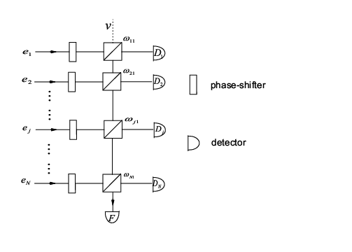
Figure 3: the OPI for filtering

III The quantum state filtering

III.1 the POVMs for the filtering

The quantum state filtering, which was termed in [21-23], is a special case of telling whether a state |Ψ?>|\Psi_{?}> belongs to , G1≡{Ψ1}G_{1}\equiv\{\Psi_{1}\} or G2≡{|Ψk>}G_{2}\equiv\{|\Psi_{k}>\} for k≥2k\geq 2, with a non-zero probability of failure. The derivation of the optimal measurement strategy, in terms of {Ei,E0}\{E_{i},E_{0}\} for i=1, 2, to distinguish |Ψ1>|\Psi_{1}> from G2G_{2} has been given and it is shown that this problem is equivalent to the discrimination of a pure state and an arbitrary mixed states. The quantum state filtering, as we shall shown, plays important roles in present works: (1) it’s an excellent example to show how our scheme works while (2) the filtering in a successive way will be used to complete other operations on G. The POVMs {Em}\{E_{m}\} for filtering are defined by E1|Ψk>=0E_{1}|\Psi_{k}>=0 for k≥2k\geq 2, E2|Ψ1>=0E_{2}|\Psi_{1}>=0 and E0E_{0} for failure, our task is to find an general unitary transformation U⁡(ω)U(\omega) which transfers each state |Ψj>|\Psi_{j}> in the ”out-space” in way like:

|Ψ1>o​u​t\displaystyle|\Psi_{1}>^{out} =\displaystyle= d11|D1>+f1|F>,\displaystyle d_{11}|D_{1}>+f_{1}|F>, (3.1)
|Ψk>o​u​t\displaystyle|\Psi_{k}>^{out} =\displaystyle= ∑j=2Ndk​j|Dj>+fk|F>.\displaystyle\sum_{j=2}^{N}d_{kj}|D_{j}>+f_{k}|F>. (3.2)

This U⁡(ω)U(\omega) can be realized by the OPI in Fig.3. Keeping in mind that |Ψk>|\Psi_{k}> has no input along the rail e1e_{1}, the input state should be |Ψ1>|\Psi_{1}> when the detector D1D_{1} has been triggered. By applying Eqs.(2.9-14), we are always possible to prevent the signals of |Ψ1>|\Psi_{1}> from appearing in the detector DkD_{k}. Usually, a complex parameter, say, ci​jc_{ij} may be expressed as

ci​j=|ci​j|​exp⁡{i​ϕi​j},c_{ij}=|c_{ij}|\exp\{i\phi_{ij}\}, (3.3)

with exp⁡{i​ϕi​j}=ci​j/|ci​j|\exp\{i\phi_{ij}\}=c_{ij}/|c_{ij}|. In Fig.3, a phase-shifter, Φi​j\Phi_{ij}, is placed in front of a beam-splitter denoted by ωi​j\omega_{ij}, we always choose the phase-shifter

Φj​1=−ϕ1​j,\Phi_{j1}=-\phi_{1j}, (3.4)

while each beam-splitter takes the value

sin⁡ωk​1\displaystyle\sin\omega_{k1} =\displaystyle= ∑j=1k−1|c1​j|2−c112​sin2⁡ω∑j=1k|c1​j|2−c112​sin2⁡ω,\displaystyle\frac{\sqrt{\sum_{j=1}^{k-1}|c_{1j}|^{2}-c^{2}_{11}\sin^{2}\omega}}{\sqrt{\sum_{j=1}^{k}|c_{1j}|^{2}-c^{2}_{11}\sin^{2}\omega}}, (3.5)
cos⁡ωk​1\displaystyle\cos\omega_{k1} =\displaystyle= |c1​k|∑j=1k|c1​j|2−c112​sin2⁡ω,\displaystyle\frac{|c_{1k}|}{\sqrt{\sum_{j=1}^{k}|c_{1j}|^{2}-c^{2}_{11}\sin^{2}\omega}}, (3.6)

with ω11≡ω\omega_{11}\equiv\omega and ci​j=<ei|Ψ>c_{ij}=<e_{i}|\Psi>, for examples,

c11\displaystyle c_{11} =\displaystyle= t1,c12=−o21⊥​t11−|o12⊥|2,\displaystyle t_{1},~~c_{12}=-\frac{o^{\bot}_{21}t_{1}}{\sqrt{1-|o^{\bot}_{12}|^{2}}}, (3.7)
c21\displaystyle c_{21} =\displaystyle= 0,c22=t21−|o12⊥|2.\displaystyle 0,~~c_{22}=\frac{t_{2}}{\sqrt{1-|o^{\bot}_{12}|^{2}}}. (3.8)

In Fig.3, we could read

|D1>i​n=exp{−iΦ11}U2−1(ω11)|D1>,|D_{1}>^{in}=\exp\{-i\Phi_{11}\}U^{-1}_{2}(\omega_{11})|D_{1}>, (3.9)

and get

|D1>i​n=−sinω|e1>+sinω|v>,|D_{1}>^{in}=-\sin\omega|e_{1}>+\sin\omega|v>, (3.10)

where Φ11=0\Phi_{11}=0 and Eq.(2.9) have been used. Through a similar argument, we could arrive at

|D2>i​n\displaystyle|D_{2}>^{in} =\displaystyle= |D2>e+cosω21sinω|v>,\displaystyle|D_{2}>^{e}+\cos\omega_{21}\sin\omega|v>, (3.11)
|D2>e\displaystyle|D_{2}>^{e} =\displaystyle= −sin⁡ω21​e−i​Φ21|e2>+cos⁡ω21​cos⁡ω|e1>,\displaystyle-\sin\omega_{21}e^{-i\Phi_{21}}|e_{2}>+\cos\omega_{21}\cos\omega|e_{1}>,

it can be proved that

|D2>e=−cos⁡ω​ei​ϕ12cos2⁡ω+sin2⁡ω​|o12⊥|2|Ψ2⊥>.|D_{2}>^{e}=\frac{-\cos\omega e^{i\phi_{12}}}{\sqrt{\cos^{2}\omega+\sin^{2}\omega|o^{\bot}_{12}|^{2}}}|\Psi_{2}^{\bot}>. (3.12)

In fact, we may use the relation, E2(ω)=I e−E1(ω)−E0(ω)E_{2}(\omega)=\textbf{I }^{e}-E_{1}({\omega})-E_{0}(\omega), instead of giving all |Dk>e|D_{k}>^{e} in detail. Using Eq.(3.1) and Eq.(3.11), we may get

|D1>e\displaystyle|D_{1}>^{e} =\displaystyle= −sin⁡ω|Ψ1⊥>,\displaystyle-\sin\omega|\Psi^{\bot}_{1}>, (3.13)
|F>e\displaystyle|F>^{e} =\displaystyle= (Ie−|D1>e<D1|)|Ψ1><Ψ1|(Ie−|D1>e<D1|)|Ψ1>,\displaystyle\frac{(\textbf{I}^{e}-|D_{1}>^{e}<D_{1}|)|\Psi_{1}>}{\sqrt{<\Psi_{1}|(\textbf{I}^{e}-|D_{1}>^{e}<D_{1}|)|\Psi_{1}>}},

and the POVMs of filtering should be

E1​(ω)\displaystyle E_{1}(\omega) =\displaystyle= |D1>e<D1|,E0(ω)=|F>e<F|,\displaystyle|D_{1}>^{e}<D_{1}|,~E_{0}(\omega)=|F>^{e}<F|, (3.14)
E2​(ω)\displaystyle E_{2}(\omega) =\displaystyle= ∑k=2N|Dk>e<Dk|=Ie−E1(ω)−E0(ω).\displaystyle\sum_{k=2}^{N}|D_{k}>^{e}<D_{k}|=\textbf{I}^{e}-E_{1}(\omega)-E_{0}(\omega).

If the POVMs {Em}\{E_{m}\} were known, then the calculation of the optimal value of filtering should be easily completed. Suppose ηj\eta_{j} is the a​𝑝𝑟𝑖𝑜𝑟𝑖{\sl a~priori} probability of |Ψj>|\Psi_{j}>, we denote P1/(N−1)​(ω)P_{1/(N-1)}(\omega) and F1/(N1)​(ω)F_{1/(N_{1})}(\omega) the average value of success and failure of filtering, respectively,

P1/(N−1)​(ω)\displaystyle P_{1/(N-1)}(\omega) =\displaystyle= ∑i=12T​r​(Ei​ρi),\displaystyle\sum_{i=1}^{2}Tr(E_{i}\rho_{i}),
F1/(N−1)​(ω)\displaystyle F_{1/(N-1)}(\omega) =\displaystyle= T​r​(E0​ρ),\displaystyle Tr(E_{0}\rho), (3.15)
P1/(N−1)​(ω)\displaystyle P_{1/(N-1)}(\omega) +\displaystyle+ F1/(N−1)​(ω)=∑j=1Nηj,\displaystyle F_{1/(N-1)}(\omega)=\sum_{j=1}^{N}\eta_{j}, (3.16)

with ρ1=η1|Ψ1><ψ1|\rho_{1}=\eta_{1}|\Psi_{1}><\psi_{1}|, ρ2=∑k=2Nηk|Ψk><Ψk|\rho_{2}=\sum_{k=2}^{N}\eta_{k}|\Psi_{k}><\Psi_{k}| and ρ=ρ1+ρ2\rho=\rho_{1}+\rho_{2}. A simple calculation shows that

F1/(N−1)​(ω)=η1​|f1|2+∑k=2Nηk​|fk|2,F_{1/(N-1)}(\omega)=\eta_{1}|f_{1}|^{2}+\sum_{k=2}^{N}\eta_{k}|f_{k}|^{2}, (3.17)

with fj=<F|ψj>f_{j}=<F|\psi_{j}> and

f1=1−t12​sin2⁡ω,fk=o1​k1−t12​sin2⁡ω.f_{1}=\sqrt{1-t_{1}^{2}\sin^{2}\omega},~f_{k}=\frac{o_{1k}}{\sqrt{1-t_{1}^{2}\sin^{2}\omega}}. (3.18)

The optimal value of F1/(N−1)​(ω)F_{1/(N-1)}(\omega), F1/(N−1)o​p​t​(ω)=F1/(N−1)​(ωo​p​t)F^{opt}_{1/(N-1)}(\omega)=F_{1/(N-1)}(\omega^{opt}), is defined to be minimum value of F1/(N−1)​(ω)F_{1/(N-1)}(\omega) in the domain of 0≤ω<2​π0\leq\omega<2\pi. From Eqs.(3.17-18), there is

d​F1/(N−1)​(ω)d​ω=t12​sin⁡2​ω​(η1−∑k=2ηk​|o1​k|21−t12​sin2⁡ω),\frac{dF_{1/(N-1)}(\omega)}{d\omega}=t_{1}^{2}\sin 2\omega(\eta_{1}-\frac{\sum_{k=2}\eta_{k}|o_{1k}|^{2}}{1-t_{1}^{2}\sin^{2}\omega}), (3.19)

and F1/(N−1)o​p​t​(ω)F^{opt}_{1/(N-1)}(\omega) happens at d​F1/(N−1)​(ω)/d​ω|ω=ωo​p​t=0.dF_{1/(N-1)}(\omega)/d\omega|_{\omega=\omega^{opt}}=0. Now, we are able to give the optimal values of filtering: (a) if ∑k=2Nηkη1​|o1​k|2>1\sqrt{\sum_{k=2}^{N}\frac{\eta_{k}}{\eta_{1}}|o_{1k}|^{2}}>1, by letting sin2⁡ωo​p​t=0\sin^{2}\omega^{opt}=0, we have

F1/(N−1)o​p​t​(ω)=η1+∑k=1N|O1​k|2,F^{opt}_{1/(N-1)}(\omega)=\eta_{1}+\sum_{k=1}^{N}|O_{1k}|^{2}, (3.20)

(b) if 1−t12≤∑k=2Nηkη1​|o1​k|2≤11-t_{1}^{2}\leq\sqrt{\sum_{k=2}^{N}\frac{\eta_{k}}{\eta_{1}}|o_{1k}|^{2}}\leq 1, through letting

sin⁡ωo​p​t=1−∑k=2Nηkη1​|o1​k|2t12,\sin\omega^{opt}=\frac{1-\sqrt{\sum_{k=2}^{N}\frac{\eta_{k}}{\eta_{1}}|o_{1k}|^{2}}}{t_{1}^{2}}, (3.21)

we arrive at

F1/(N−1)o​p​t​(ω)=2​η1​∑k=2Nηk​|o1​k|2,F^{opt}_{1/(N-1)}(\omega)=2\sqrt{\eta_{1}\sum_{k=2}^{N}\eta_{k}|o_{1k}|^{2}}, (3.22)

and (c) if ∑k=2Nηkη1​|o1​k|2<1−t12\sqrt{\sum_{k=2}^{N}\frac{\eta_{k}}{\eta_{1}}|o_{1k}|^{2}}<1-t_{1}^{2}, the optimal value should be

F1/(N−1)o​p​t​(ω)=η1​(1−t12)+∑k=2Nηk​|o1​k|21−t12,F^{opt}_{1/(N-1)}(\omega)=\eta_{1}(1-t_{1}^{2})+\frac{\sum_{k=2}^{N}\eta_{k}|o_{1k}|^{2}}{1-t_{1}^{2}}, (3.23)

while sin2⁡ωo​p​t=1.\sin^{2}\omega^{opt}=1. Substituting ωo​p​t\omega^{opt} for ω\omega in Eqs.(3.13-14), we could also get the optimal POVMs {Emo​p​t}\{E^{opt}_{m}\}.

III.2 an example: filtering for N=3

The filtering of N=3 is a case with a fully analytical solution and an optical implementation of the optimal strategy [23], we shall show, via a simple optical setting, how to recover all the optimal values in [23]. For N=3, there is

1−t12=|o12|2+|o13|2−o12​o23​o31−o21​o13​o321−|o23|2.1-t_{1}^{2}=\frac{|o_{12}|^{2}+|o_{13}|^{2}-o_{12}o_{23}o_{31}-o_{21}o_{13}o_{32}}{1-|o_{23}|^{2}}. (3.24)

Defining

A=η2​|o12|2+η3​|o13|2,A=\eta_{2}|o_{12}|^{2}+\eta_{3}|o_{13}|^{2}, (3.25)

we can write the general results of filtering to the N=3: (a) for A>η1A>\eta_{1}, there is

F1/2o​p​t=η1+A,F^{opt}_{1/2}=\eta_{1}+A, (3.26)

(b) for η1​(1−t12)2≤A≤η1\eta_{1}(1-t_{1}^{2})^{2}\leq A\leq\eta_{1}, there should be

F1/2o​p​t=2​η1​A,F^{opt}_{1/2}=2\sqrt{\eta_{1}A}, (3.27)

and (c) else, A<η1​(1−t12)2A<\eta_{1}(1-t_{1}^{2})^{2},

F1/2o​p​t=η1​(1−t12)+A1−t12.F^{opt}_{1/2}=\eta_{1}(1-t_{1}^{2})+\frac{A}{1-t_{1}^{2}}. (3.28)

Besides all this optimal results, we could also get the optimal POVMs for filtering with N=3.
Refer to caption
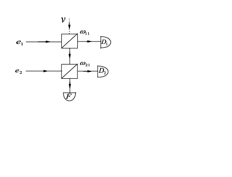
Figure 4: the OPI for filtering with N=2

III.3 filtering with N=2: discriminating two pure states

The problem, how to discriminate |Ψ1>|\Psi_{1}> from |Ψ2>|\Psi_{2}>, is the most interesting case in the field of quantum states unambiguously discrimination. Here, it can be solved as a special case of filtering with N=2. The present solution is complete in the sense that: not only the optimal values but also the optimal POVMs should be given at the same time while the POVMs have the forms required by Eqs.(2.2-4). The OPI in Fig.4 is for the filtering with N=2 and it takes <Ψ1|Ψ2>=<Ψ2|Ψ1><\Psi_{1}|\Psi_{2}>=<\Psi_{2}|\Psi_{1}> for simplicity. From the DTR for N=2, the basis vectors should be

|e1>=|Ψ1⊥>,|e2>=|Ψ2>,|e_{1}>=|\Psi_{1}^{\bot}>,~~|e_{2}>=|\Psi_{2}>, (3.29)

and the states have the forms

|Ψ1>\displaystyle|\Psi_{1}> =\displaystyle= 1−|o12|2|e1>+o21|e2>,\displaystyle\sqrt{1-|o_{12}|^{2}}|e_{1}>+o_{21}|e_{2}>,
|Ψ2>\displaystyle|\Psi_{2}> =\displaystyle= |e2>.\displaystyle|e_{2}>. (3.30)

With known parameters for N=2, which have been given in the Appendix, we have

|ψ1⊥>\displaystyle|\psi_{1}^{\bot}> =\displaystyle= |Ψ1>−o21|Ψ2>1−|o12|2,\displaystyle\frac{|\Psi_{1}>-o_{21}|\Psi_{2}>}{\sqrt{1-|o_{12}|^{2}}},
|ψ2⊥>\displaystyle|\psi_{2}^{\bot}> =\displaystyle= |Ψ2>−o12|Ψ1>1−|o12|2,\displaystyle\frac{|\Psi_{2}>-o_{12}|\Psi_{1}>}{\sqrt{1-|o_{12}|^{2}}}, (3.31)

by applying Eq.(2.25). The POVMs for discriminating two linearly independent states, |Ψ1>|\Psi_{1}> and |Ψ1>|\Psi_{1}>, should be

E1\displaystyle E_{1} =\displaystyle= sin2ω|Ψ⊥1><ψ1⊥|,\displaystyle\sin^{2}\omega|\Psi^{\bot}_{1}><\psi_{1}^{\bot}|,
E2\displaystyle E_{2} =\displaystyle= cos2⁡ωcos2⁡ω+sin2⁡ω​|o12|2|Ψ⊥2><ψ2⊥|,\displaystyle\frac{\cos^{2}\omega}{\cos^{2}\omega+\sin^{2}\omega|o_{12}|^{2}}|\Psi^{\bot}_{2}><\psi_{2}^{\bot}|, (3.32)
E0\displaystyle E_{0} =\displaystyle= (|Ψ1>−t12sin2ω|Ψ⊥1>)(<Ψ1|−t12sin2ω<Ψ⊥1|)1−t12​sin2⁡ω\displaystyle\frac{(|\Psi_{1}>-t_{1}^{2}\sin^{2}\omega|\Psi^{\bot}_{1}>)(<\Psi_{1}|-t_{1}^{2}\sin^{2}\omega<\Psi^{\bot}_{1}|)}{1-t^{2}_{1}\sin^{2}\omega}

while t1=1−|o12|2t_{1}=\sqrt{1-|o_{12}|^{2}}, and

F1/1​(ω)=η1​(1−t12​sin2⁡ω)+η2​|o12|21−t12​sin2⁡ω.F_{1/1}(\omega)=\eta_{1}(1-t_{1}^{2}\sin^{2}\omega)+\frac{\eta_{2}|o_{12}|^{2}}{1-t_{1}^{2}\sin^{2}\omega}. (3.33)

Now, we could give the optimal values and the optimal POVMs at the same time: (1) for η2η1>1|o12|\sqrt{\frac{\eta_{2}}{\eta_{1}}}>\frac{1}{|o_{12}|}, let sin2⁡ωo​p​t=0\sin^{2}\omega^{opt}=0, there should be

E1o​p​t\displaystyle E_{1}^{opt} =\displaystyle= 0,E2o​p​t=|Ψ2⊥><Ψ⊥2|,\displaystyle 0,~~E_{2}^{opt}=|\Psi_{2}^{\bot}><\Psi^{\bot}_{2}|,
E0o​p​t\displaystyle E_{0}^{opt} =\displaystyle= |Ψ1><Ψ1|,\displaystyle|\Psi_{1}><\Psi_{1}|,
F1/1o​p​t​(ω)\displaystyle F_{1/1}^{opt}(\omega) =\displaystyle= η1+η2​|o12|2,\displaystyle\eta_{1}+\eta_{2}|o_{12}|^{2}, (3.34)
P1/1o​p​t​(ω)\displaystyle P_{1/1}^{opt}(\omega) =\displaystyle= η2​(1−|o12|2),\displaystyle\eta_{2}(1-|o_{12}|^{2}),

(2) if |o12|≤η2η1≤1|o12||o_{12}|\leq\sqrt{\frac{\eta_{2}}{\eta_{1}}}\leq\frac{1}{|o_{12}|}, by letting

sin2⁡ωo​p​t=1−η2η1​|o12|1−|o12|2,\sin^{2}\omega^{opt}=\frac{1-\sqrt{\frac{\eta_{2}}{\eta_{1}}}|o_{12}|}{1-|o_{12}|^{2}}, (3.35)

we shall get the optimal POVMs

E1o​p​t\displaystyle E_{1}^{opt} =\displaystyle= 1−η2η1​|o12|1−|o12|2|Ψ⊥1><Ψ1⊥|,\displaystyle\frac{1-\sqrt{\frac{\eta_{2}}{\eta_{1}}}|o_{12}|}{1-|o_{12}|^{2}}|\Psi^{\bot}_{1}><\Psi_{1}^{\bot}|,
E2o​p​t\displaystyle E_{2}^{opt} =\displaystyle= 1−η1η2​|o12|1−|o12|2|Ψ⊥2><Ψ2⊥|,\displaystyle\frac{1-\sqrt{\frac{\eta_{1}}{\eta_{2}}}|o_{12}|}{1-|o_{12}|^{2}}|\Psi^{\bot}_{2}><\Psi_{2}^{\bot}|,
E0o​p​t\displaystyle E_{0}^{opt} =\displaystyle= Ie−∑j=12Ejo​p​t,\displaystyle\textbf{I}^{e}-\sum_{j=1}^{2}E_{j}^{opt}, (3.36)

which give the optimal results

F1/1o​p​t​(ω)\displaystyle F_{1/1}^{opt}(\omega) =\displaystyle= 2​η1​η2​|o12|,\displaystyle 2\sqrt{\eta_{1}\eta_{2}}|o_{12}|, (3.37)
P1/1o​p​t​(ω)\displaystyle P_{1/1}^{opt}(\omega) =\displaystyle= ∑j=12ηj−2​η1​η2​|o12|,\displaystyle\sum_{j=1}^{2}\eta_{j}-2\sqrt{\eta_{1}\eta_{2}}|o_{12}|,

and (3) when η2η1<|o12|,\sqrt{\frac{\eta_{2}}{\eta_{1}}}<|o_{12}|,, through choosing sin2⁡ωo​p​t=1\sin^{2}\omega^{opt}=1, we arrive at

E1o​p​t=|Ψ1⊥><Ψ1⊥|,E0o​p​t=|Ψ2><Ψ2|,E_{1}^{opt}=|\Psi_{1}^{\bot}><\Psi_{1}^{\bot}|,~E_{0}^{opt}=|\Psi_{2}><\Psi_{2}|, (3.38)

while E2o​p​t=0E_{2}^{opt}=0, all these operators leads to

F1/1o​p​t​(ω)\displaystyle F_{1/1}^{opt}(\omega) =\displaystyle= η1​|o12|2+η2,\displaystyle\eta_{1}|o_{12}|^{2}+\eta_{2}, (3.39)
P1/1o​p​t​(ω)\displaystyle P_{1/1}^{opt}(\omega) =\displaystyle= η1​(1−|o12|2).\displaystyle\eta_{1}(1-|o_{12}|^{2}).

Compare with other methods of solving the same question, the present scheme states that the general POVMs may be given before the decision of the optimal values of success and failure.

IV filtering in subspace

IV.1 filtering with the background
Refer to caption
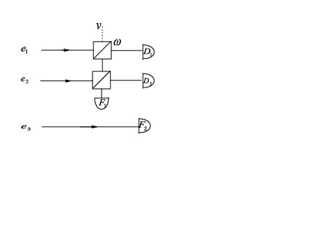
Figure 5: The OPI for discriminating two states with the background

Suppose G1≡{|Ψk>}G_{1}\equiv\{|\Psi_{k}>\} and G2≡{|Ψl>},G_{2}\equiv\{|\Psi_{l}>\}, a new operation of G can be specified by the definition of the POVMs as E1|Ψ?>=0E_{1}|\Psi_{?}>=0 if |Ψ?>|\Psi_{?}> belongs to G2G_{2}, E2|Ψ?>=0E_{2}|\Psi_{?}>=0 if |Ψ?>|\Psi_{?}> belongs to G1G_{1} and E0E_{0} corresponds to failure. If a state, say, |Ψg>|\Psi_{g}>, is shared by both G1G_{1} and G2G_{2}, then E1|Ψg>=E2|Ψg>=0E_{1}|\Psi_{g}>=E_{2}|\Psi_{g}>=0 according to the definition of the POVMs {Em}\{E_{m}\}. We call this case the name of discriminating with the background. In this section, we shall consider a simple case of discriminating |Ψ1>|\Psi_{1}> from |Ψ2>|\Psi_{2}> with |Ψ3>|\Psi_{3}> as the background. In the DTR, this operation on G can also be viewed as a filtering in a two-dimensional subspace.

For N=3, the the basis vectors in the DTR should be:

|e1>\displaystyle|e_{1}> =\displaystyle= |Ψ1⊥>,\displaystyle|\Psi_{1}^{\bot}>,
|e2>\displaystyle|e_{2}> =\displaystyle= |Ψ2⊥>−o⊥12|Ψ1⊥>1−|o12⊥|2,\displaystyle\frac{|\Psi_{2}^{\bot}>-o^{\bot}_{12}|\Psi_{1}^{\bot}>}{\sqrt{1-|o_{12}^{\bot}|^{2}}}, (4.1)
|e3>\displaystyle|e_{3}> =\displaystyle= |Ψ3>,\displaystyle|\Psi_{3}>,

with

o12⊥=o13​o32−o12(1−|o23|2)​(1−|o13|2),o_{12}^{\bot}=\frac{o_{13}o_{32}-o_{12}}{\sqrt{(1-|o_{23}|^{2})(1-|o_{13}|^{2})}}, (4.2)

while the matrix C(3) takes the form

(t1o12−o13​o321−|o32|2o3101−|o32|2o32001),\left(\begin{array}[]{ccc}t_{1}&\frac{o_{12}-o_{13}o_{32}}{\sqrt{1-|o_{32}|^{2}}}&o_{31}\\ 0&\sqrt{1-|o_{32}|^{2}}&o_{32}\\ 0&0&1\\ \end{array}\right), (4.3)

with t1t_{1}, which holds for N=3, is

t1=det(O⁡(3))1−|o23|2.t_{1}=\sqrt{\frac{\det(O(3))}{1-|o_{23}|^{2}}}. (4.4)

The U⁡(ω)U(\omega) in Fig.5 is required to transform each |Ψj>|\Psi_{j}> to |Ψj>o​u​t|\Psi_{j}>^{out} as

|Ψ1>o​u​t\displaystyle|\Psi_{1}>^{out} =\displaystyle= d1|D1>+f11|F1>+f12|F2>,\displaystyle d_{1}|D_{1}>+f_{11}|F_{1}>+f_{12}|F_{2}>,
|Ψ2>o​u​t\displaystyle|\Psi_{2}>^{out} =\displaystyle= d2|D2>+f21|F1>+f22|F2>,\displaystyle d_{2}|D_{2}>+f_{21}|F_{1}>+f_{22}|F_{2}>, (4.5)
|Ψ3>o​u​t\displaystyle|\Psi_{3}>^{out} =\displaystyle= |F2>,\displaystyle|F_{2}>,

and this goal can be reached, as we shall shown later, by applying the argument of filtering. The U−1​(ω)U^{-1}(\omega) shall give

|D1>e\displaystyle|D_{1}>^{e} =\displaystyle= −sin⁡ω|Ψ1⊥>,\displaystyle-\sin\omega|\Psi^{\bot}_{1}>,
|F2>e\displaystyle|F_{2}>^{e} =\displaystyle= |Ψ3>,\displaystyle|\Psi_{3}>, (4.6)
|F1>e\displaystyle|F_{1}>^{e} =\displaystyle= (Ie−|F2>e<F2|−|D1>e<D1|)|Ψ1>1−|f12|2−|d1|2,\displaystyle\frac{(I^{e}-|F_{2}>^{e}<F_{2}|-|D_{1}>^{e}<D_{1}|)|\Psi_{1}>}{\sqrt{1-|f_{12}|^{2}-|d_{1}|^{2}}},

with |D2>e|D_{2}>^{e} has given by Eq.(3.12). The POVMs are defined by

E1​(ω)\displaystyle E_{1}(\omega) =\displaystyle= |D1>e<D1|,E2(ω)=|D2>e<D2|,\displaystyle|D_{1}>^{e}<D_{1}|,~~E_{2}(\omega)=|D_{2}>^{e}<D_{2}|,
E0​(ω)\displaystyle E_{0}(\omega) =\displaystyle= |F1>e<F1|+|F1>e<F1|.\displaystyle|F_{1}>^{e}<F_{1}|+|F_{1}>^{e}<F_{1}|. (4.7)

Defining

F1​(ω)\displaystyle F_{1}(\omega) =\displaystyle= ∑j=12ηj​|fj​1|2,\displaystyle\sum_{j=1}^{2}\eta_{j}|f_{j1}|^{2}, (4.8)
F2​(ω)\displaystyle F_{2}(\omega) =\displaystyle= ∑i=13ηi​|fi​2|2,\displaystyle\sum_{i=1}^{3}\eta_{i}|f_{i2}|^{2}, (4.9)

with fi​j=<Fj|Ψi>f_{ij}=<F_{j}|\Psi_{i}>, the average value of failure should be

F⁡(ω)=F1​(ω)+F2​(ω).F(\omega)=F_{1}(\omega)+F_{2}(\omega). (4.10)

A simple calculation shows

F2​(ω)=∑j=12ηj​|o3​j|2+η3,F_{2}(\omega)=\sum_{j=1}^{2}\eta_{j}|o_{3j}|^{2}+\eta_{3}, (4.11)

it is still in a special form of filtering with N=3, see Eq.(3.26). The F1​(ω)F_{1}(\omega) is left to be decided by the general results of filtering with N=2.

Formally, |Ψ1>|\Psi_{1}> and |Ψ1>|\Psi_{1}> can written by

|Ψ1>\displaystyle|\Psi_{1}> =\displaystyle= 1−|c13|2|Ψ1′>+c13|e3>,\displaystyle\sqrt{1-|c_{13}|^{2}}|\Psi_{1}^{\prime}>+c_{13}|e_{3}>,
|Ψ2>\displaystyle|\Psi_{2}> =\displaystyle= 1−|c23|2|Ψ2′>+c23|e3>,\displaystyle\sqrt{1-|c_{23}|^{2}}|\Psi_{2}^{\prime}>+c_{23}|e_{3}>, (4.12)

with |Ψ1′>|\Psi_{1}^{\prime}> and |Ψ2′>|\Psi_{2}^{\prime}> are two normalized states defined in the subspace specified by {|ej>}\{|e_{j}>\} for j=1,2:

|Ψ1′>\displaystyle|\Psi_{1}^{\prime}> =\displaystyle= c11|e1>+c12|e2>1−|c13|2,\displaystyle\frac{c_{11}|e_{1}>+c_{12}|e_{2}>}{\sqrt{1-|c_{13}|^{2}}},
|Ψ2′>\displaystyle|\Psi_{2}^{\prime}> =\displaystyle= |e2>,\displaystyle|e_{2}>, (4.13)

and their overlap should be

o12′=<Ψ1′|Ψ2′>=o12−o13​o32(1−|o31|2)​(1−|o32|2).o^{\prime}_{12}=<\Psi_{1}^{\prime}|\Psi_{2}^{\prime}>=\frac{o_{12}-o_{13}o_{32}}{\sqrt{(1-|o_{31}|^{2})(1-|o_{32}|^{2})}}. (4.14)

Now, in the two-dimensional subspace with {|e1>,|e2>}\{|e_{1}>,|e_{2}>\}, our task is to discriminate |Ψ1>|\Psi_{1}> from |Ψ2>|\Psi_{2}> with

ηj′=ηj​(1−|o3​j|2),\eta^{\prime}_{j}=\eta_{j}(1-|o_{3j}|^{2}), (4.15)

for j=1,2, to be their a​𝑝𝑟𝑖𝑜𝑟𝑖{\sl a~priori} probability, respectively. According to our discussion about filtering, we have

F1​(ω)\displaystyle F_{1}(\omega) =\displaystyle= η1′​(1−(1−|o12′|2)​sin2⁡ω)\displaystyle\eta^{\prime}_{1}(1-(1-|o_{12}^{\prime}|^{2})\sin^{2}\omega) (4.16)
+η2′​|o12′|21−(1−|o12′|2)​sin2⁡ω,\displaystyle+\frac{\eta_{2}^{\prime}|o_{12}^{\prime}|^{2}}{1-(1-|o_{12}^{\prime}|^{2})\sin^{2}\omega},

which is equivalent with the one given by Eq.(4.9). This is the reason why the present case is viewed as a process of filtering with N=2, certainly, in the subspace without the background. It’s optimal results have nearly the same forms for filtering with N=2: (1) for η2′η1′>1|o12′|\sqrt{\frac{\eta^{\prime}_{2}}{\eta^{\prime}_{1}}}>\frac{1}{|o^{\prime}_{12}|}, let sin2⁡ωo​p​t=0\sin^{2}\omega^{opt}=0, there should be

Fo​p​t​(ω)\displaystyle F^{opt}(\omega) =\displaystyle= F2​(ω)+η1′+η2′​|o12′|2,\displaystyle F_{2}(\omega)+\eta^{\prime}_{1}+\eta^{\prime}_{2}|o^{\prime}_{12}|^{2}, (4.17)
Po​p​t​(ω)\displaystyle P^{opt}(\omega) =\displaystyle= η2′​(1−|o12′|2),\displaystyle\eta^{\prime}_{2}(1-|o^{\prime}_{12}|^{2}),

(2) if |o12′|≤η2′η1′≤1|o12′||o^{\prime}_{12}|\leq\sqrt{\frac{\eta^{\prime}_{2}}{\eta^{\prime}_{1}}}\leq\frac{1}{|o^{\prime}_{12}|}, by letting

sin2⁡ωo​p​t=1−η2′η1′​|o12′|1−|o12′|2,\sin^{2}\omega^{opt}=\frac{1-\sqrt{\frac{\eta^{\prime}_{2}}{\eta^{\prime}_{1}}}|o^{\prime}_{12}|}{1-|o^{\prime}_{12}|^{2}}, (4.18)

we shall get the optimal results

Fo​p​t​(ω)\displaystyle F^{opt}(\omega) =\displaystyle= F2​(ω)+2​η1′​η2′​|o12′|,\displaystyle F_{2}(\omega)+2\sqrt{\eta^{\prime}_{1}\eta^{\prime}_{2}}|o^{\prime}_{12}|, (4.19)
Po​p​t​(ω)\displaystyle P^{opt}(\omega) =\displaystyle= ∑j=12ηj′−2​η1′​η2′​|o12′|,\displaystyle\sum_{j=1}^{2}\eta^{\prime}_{j}-2\sqrt{\eta^{\prime}_{1}\eta^{\prime}_{2}}|o^{\prime}_{12}|,

and (3) when η2′η1′<|o12′|,\sqrt{\frac{\eta^{\prime}_{2}}{\eta^{\prime}_{1}}}<|o^{\prime}_{12}|, through choosing sin2⁡ωo​p​t=1\sin^{2}\omega^{opt}=1, we arrive at

Fo​p​t​(ω)\displaystyle F^{opt}(\omega) =\displaystyle= F2​(ω)+η1′​|o12′|2+η2,\displaystyle F_{2}(\omega)+\eta^{\prime}_{1}|o^{\prime}_{12}|^{2}+\eta_{2}, (4.20)
Po​p​t​(ω)\displaystyle P^{opt}(\omega) =\displaystyle= η1′​(1−|o12′|2).\displaystyle\eta^{\prime}_{1}(1-|o^{\prime}_{12}|^{2}).

It should be noted that F2​(ω)F_{2}(\omega), which has been given in Eq.(4.11), is in fact a constant. The present argument, which is suitable for discriminating G1≡{|ψ1>,|Ψ3>}G_{1}\equiv\{|\psi_{1}>,|\Psi_{3}>\} and G2≡{|ψ2>,|Ψ3>}G_{2}\equiv\{|\psi_{2}>,|\Psi_{3}>\}, can be generalized to the discriminating two general mixtures sharing part of states in comm.

IV.2 discriminating two mixtures in Jordan basis
Refer to caption
Figure 6: The OPI for filtering the mixtures in Jordan basis

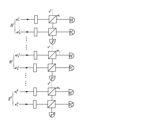
Suppose there are two mixtures,

ρ1\displaystyle\rho_{1} =\displaystyle= ∑i=1Kpi|Ψi><Ψi|,\displaystyle\sum_{i=1}^{K}p_{i}|\Psi_{i}><\Psi_{i}|,
ρ2\displaystyle\rho_{2} =\displaystyle= ∑j=K+12​Kpj|Ψj><Ψj|,\displaystyle\sum_{j=K+1}^{2K}p_{j}|\Psi_{j}><\Psi_{j}|, (4.21)

with ∑i=1Kpi=∑j=K+12​Kpj=1\sum_{i=1}^{K}p_{i}=\sum_{j=K+1}^{2K}p_{j}=1. Let λk\lambda_{k} to be the a​𝑝𝑟𝑖𝑜𝑟𝑖{\sl a~priori} probability for ρk\rho_{k}, k=1, 2, we may introduce ηi=λ1​pi\eta_{i}=\lambda_{1}p_{i} as the a​𝑝𝑟𝑖𝑜𝑟𝑖{\sl a~priori} probability for |Ψi>|\Psi_{i}> in G1≡{|Ψi>}G_{1}\equiv\{|\Psi_{i}>\} while ηj=λ2​pj\eta_{j}=\lambda_{2}p_{j} as the a​𝑝𝑟𝑖𝑜𝑟𝑖{\sl a~priori} probability for |Ψi>|\Psi_{i}> in G2≡{|Ψj>}G_{2}\equiv\{|\Psi_{j}>\}. If <Ψk|Ψk′>=0<\Psi_{k}|\Psi_{k^{\prime}}>=0 for k≠k′k\neq k^{\prime} except <Ψi|Ψi+k>=cos⁡θi<\Psi_{i}|\Psi_{i+k}>=\cos\theta_{i}, ρ1\rho_{1} and ρ2\rho_{2} are called in Jordan basis. Defining the POVMs: E1|Ψj>=E2|Ψi>=0E_{1}|\Psi_{j}>=E_{2}|\Psi_{i}>=0 while E0E_{0} for failure, this {Em}\{E_{m}\} can be get, as it has been show by the works in [21-23], through discriminating pairs of pure states in each subspace.

The OPI in Fig.5 is used to discriminate these two mixtures, ρ1\rho_{1} and ρ2\rho_{2}. The total Hilbert space here is defined by H=∑i=1K⊕HiH=\sum_{i=1}^{K}\oplus H^{i}, each HiH^{i} is a two-dimensional subspace with it’s basis as

|ei1>\displaystyle|e^{i}_{1}> =\displaystyle= |Ψi>−cosθi|ΨK+i>sin⁡θi,\displaystyle\frac{|\Psi_{i}>-\cos\theta_{i}|\Psi_{K+i}>}{\sin\theta_{i}},
|ei2>\displaystyle|e^{i}_{2}> =\displaystyle= |ΨK+i>,\displaystyle|\Psi_{K+i}>, (4.22)

the two states in this HeH^{e} are

|Ψi>\displaystyle|\Psi_{i}> =\displaystyle= sin⁡θi|e1i>+cos⁡θi|e2i>,\displaystyle\sin\theta_{i}|e^{i}_{1}>+\cos\theta_{i}|e^{i}_{2}>,
|ΨK+i>\displaystyle|\Psi_{K+i}> =\displaystyle= |ei2>,\displaystyle|e^{i}_{2}>, (4.23)

while their reciprocal states

|Ψ⊥i>\displaystyle|\Psi^{\bot}_{i}> =\displaystyle= |Ψi>−cosθi|ΨK+i>sin⁡θi,\displaystyle\frac{|\Psi_{i}>-\cos\theta_{i}|\Psi_{K+i}>}{\sin\theta_{i}},
|Ψ⊥K+i>\displaystyle|\Psi^{\bot}_{K+i}> =\displaystyle= |ΨK+i>−cosθi|Ψi>sin⁡θi.\displaystyle\frac{|\Psi_{K+i}>-\cos\theta_{i}|\Psi_{i}>}{\sin\theta_{i}}. (4.24)

In this HiH^{i}, our task is to filter |Ψi>|\Psi_{i}> from |ΨK+i>|\Psi_{K+i}>, the POVMs, {Emi}\{E^{i}_{m}\}, to complete this task should be

E1i​(ωi)\displaystyle E_{1}^{i}(\omega_{i}) =\displaystyle= sin2ωi|Ψ⊥i><Ψ⊥i|,,\displaystyle\sin^{2}\omega_{i}|\Psi^{\bot}_{i}><\Psi^{\bot}_{i}|,,
E2i​(ωi)\displaystyle E_{2}^{i}(\omega_{i}) =\displaystyle= cos2⁡ωicos2⁡ωi+sin2⁡ωi​cos2⁡θi|ΨK+i⊥]><ΨK+i⊥|,\displaystyle\frac{\cos^{2}\omega_{i}}{\cos^{2}\omega_{i}+\sin^{2}\omega_{i}\cos^{2}\theta_{i}}|\Psi^{\bot}_{K+i}]><\Psi^{\bot}_{K+i}|,
E0i​(ωi)\displaystyle E_{0}^{i}(\omega_{i}) =\displaystyle= Ii−∑k=12Eki​(ωi),\displaystyle\textbf{I}^{i}-\sum_{k=1}^{2}E^{i}_{k}(\omega_{i}), (4.25)

the average value of the failure in HiH^{i} should be

Fi​(ωi)\displaystyle F^{i}(\omega_{i}) =\displaystyle= ηi​(1−sin2⁡θi​sin2⁡ωi)\displaystyle\eta_{i}(1-\sin^{2}\theta_{i}\sin^{2}\omega_{i}) (4.26)
+ηK+i​cos2⁡θi1−sin2⁡θi​sin2⁡ωi,\displaystyle+\frac{\eta_{K+i}\cos^{2}\theta_{i}}{1-\sin^{2}\theta_{i}\sin^{2}\omega_{i}},

it’s optical values are given by the theorem of filtering with N=2. Finally, we can define the POVMs {Em}\{E_{m}\} by

Em=∑i=1KEmi,E_{m}=\sum_{i=1}^{K}E^{i}_{m}, (4.27)

for m=0, 1, 2. The average value of fail can be expressed by

F⁡(ω)=∑i=1KFi​(ωi),F(\omega)=\sum_{i=1}^{K}F^{i}(\omega_{i}), (4.28)

while it’s optimal value

Fo​p​t​(ω)=∑i=1KFi​(ωi=ωio​p​t),F^{opt}(\omega)=\sum_{i=1}^{K}F^{i}(\omega_{i}=\omega_{i}^{opt}), (4.29)

where ωio​p​t\omega_{i}^{opt} should depend on the actual value of the parameters, ηi\eta_{i}, ηK+i\eta_{K+i} and cos⁡θi\cos\theta_{i}, here, this requirement has also been pointed by the recent work [20].
Refer to caption
Figure 7: the OPI for discriminating three pure stats

V The successive filtering for discrimination of pure states

V.1 the optical realization of U⁡(ω)U(\omega)

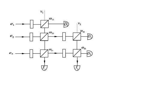
In present section, we shall show the POVMs, which are defined for discriminating of pure states, can be realized in an enlarged Hilbert space by applying the successive filtering. The OPI in Fig.7 is designed to discriminate three linearly independent states, |Ψi>|\Psi_{i}> for i=1, 2, 3, here. The U⁡(ω)U(\omega) realized by this OPI can be written as

U⁡(ω)=R⁡(2)​R​(1),U(\omega)=R(2)R(1), (5.1)

with R(1) denotes the unitary transformation done by the beam-splitters and phase-shifters, ωj​1\omega_{j1} and Φj​1\Phi_{j1} for j=1, 2, 3, on the left part of Fig.7, while R(2) denotes the unitary transformation realizes by, ωk​1\omega_{k1} and Φk​1\Phi_{k1} for k=2, 3, the beam-splitters and phase-shifters on the right part. At first, the R(1) is defined to filter |Ψ1>|\Psi_{1}> from the states, |Ψ2>|\Psi_{2}> and |Ψ3>|\Psi_{3}>, here.

R⁡(1)|Ψ1>\displaystyle R(1)|\Psi_{1}> =\displaystyle= d11|D1>+f11|F1>,\displaystyle d_{11}|D_{1}>+f_{11}|F_{1}>, (5.2)
R⁡(1)|Ψk>\displaystyle R(1)|\Psi_{k}> =\displaystyle= 1−|fk​1|2|Ψk′>+fk​1|F1>,\displaystyle\sqrt{1-|f_{k1}|^{2}}|\Psi^{\prime}_{k}>+f_{k1}|F_{1}>,

for k=2, 3, while |Ψk′>|\Psi_{k}^{\prime}> lies in a two-dimensional subspace H’, which is specified by it’s basis as {|ωk​1,r>}\{|\omega_{k1},r>\} for k=2, 3, and

|Ψ2′>\displaystyle|\Psi_{2}^{\prime}> =\displaystyle= 1−|o23′|2|ω21,r>+o32′|Ψ3′>,\displaystyle\sqrt{1-|o^{\prime}_{23}|^{2}}|\omega_{21},r>+o^{\prime}_{32}|\Psi_{3}^{\prime}>,
|Ψ3′>\displaystyle|\Psi_{3}^{\prime}> =\displaystyle= ei​ϕ3′|ω31,r>,\displaystyle e^{i\phi_{3}^{\prime}}|\omega_{31},r>, (5.3)

where o23′=<Ψ2′|Ψ3′>o_{23}^{\prime}=<\Psi_{2}^{\prime}|\Psi^{\prime}_{3}>, using Eq.(5.2), we get

o23′=o23−f21∗​f31(1−|f21|2)​(1−|f31|2),o^{\prime}_{23}=\frac{o_{23}-f^{*}_{21}f_{31}}{\sqrt{(1-|f_{21}|^{2})(1-|f_{31}|^{2})}}, (5.4)

In this run of filtering, the average value of fail should be

F1​(ω)=∑j=13ηj​|fj​1|2,F_{1}(\omega)=\sum_{j=1}^{3}\eta_{j}|f_{j1}|^{2}, (5.5)

with fj​1=<F1|Ψj>f_{j1}=<F_{1}|\Psi_{j}>. After the first turn of filtering, we are left with two states, |Ψ′2>|\Psi^{\prime}_{2}> and |Ψ′3>|\Psi^{\prime}_{3}> in H’, with their a​𝑝𝑟𝑖𝑜𝑟𝑖{\sl a~priori} probabilities to be

ηk′=ηk​(1−|fk​1|2),\eta^{\prime}_{k}=\eta_{k}(1-|f_{k1}|^{2}), (5.6)

for k=2, 3, respectively. R(2) is designed to filter |Ψ′2>|\Psi^{\prime}_{2}> from |Ψ′3>|\Psi^{\prime}_{3}> in the way like:

R⁡(2)|Ψ2′>\displaystyle R(2)|\Psi_{2}^{\prime}> =\displaystyle= 11−|f21|2(d22|D2>+f22|F2>),\displaystyle\frac{1}{\sqrt{1-|f_{21}|^{2}}}(d_{22}|D_{2}>+f_{22}|F_{2}>),
R⁡(2)|Ψ3′>\displaystyle R(2)|\Psi_{3}^{\prime}> =\displaystyle= 11−|f31|2(d33|D3>+f32|F2>),\displaystyle\frac{1}{\sqrt{1-|f_{31}|^{2}}}(d_{33}|D_{3}>+f_{32}|F_{2}>),

and in this run of filtering, the average value of the failure should be

F2​(ω)\displaystyle F_{2}(\omega) =\displaystyle= η2′​(1−(1−|o23′|2)​sin2⁡ω2)\displaystyle\eta_{2}^{\prime}(1-(1-|o_{23}^{\prime}|^{2})\sin^{2}\omega_{2}) (5.8)
+η3′​|o23′|21−(1−|o23′|2)​sin2⁡ω2,\displaystyle+\frac{\eta_{3}^{\prime}|o_{23}^{\prime}|^{2}}{1-(1-|o_{23}^{\prime}|^{2})\sin^{2}\omega_{2}},

with ω22≡ω2\omega_{22}\equiv\omega_{2}. If

η2=η3=η,|f21|=|f31|,\eta_{2}=\eta_{3}=\eta,~~|f_{21}|=|f_{31}|, (5.9)

then we shall get

F2o​p​t=2​η​|o23−f21∗​f31|,F_{2}^{opt}=2\eta|o_{23}-f^{*}_{21}f_{31}|, (5.10)

by letting

sin2⁡ω2o​p​t=1−|o23′|1−|o23′|2.\sin^{2}\omega_{2}^{opt}=\frac{1-|o^{\prime}_{23}|}{1-|o^{\prime}_{23}|^{2}}. (5.11)

V.2 the POVMs for discriminating three pure states

By performing the R(2) after R(1), the state |Ψj>|\Psi_{j}> are transformed into:

|Ψ1>o​u​t\displaystyle|\Psi_{1}>^{out} =\displaystyle= d11|D1>+f11|F1>,\displaystyle d_{11}|D_{1}>+f_{11}|F_{1}>,
|Ψ2>o​u​t\displaystyle|\Psi_{2}>^{out} =\displaystyle= d22|D2>+f21|F1>+f22|F2>,\displaystyle d_{22}|D_{2}>+f_{21}|F_{1}>+f_{22}|F_{2}>, (5.12)
|Ψ3>o​u​t\displaystyle|\Psi_{3}>^{out} =\displaystyle= d33|D3>+f31|F1>+f32|F2>.\displaystyle d_{33}|D_{3}>+f_{31}|F_{1}>+f_{32}|F_{2}>.

With U−1​(ω)=R−1​(1)​R−1​(2)U^{-1}(\omega)=R^{-1}(1)R^{-1}(2), we can arrive at

|D1>e\displaystyle|D_{1}>^{e} =\displaystyle= −sin⁡ω1|ψ1⊥>,\displaystyle-\sin\omega_{1}|\psi^{\bot}_{1}>,
|D2>e\displaystyle|D_{2}>^{e} =\displaystyle= cosω1sinω2cos⁡ω12+sin2⁡ω1​|o12⊥|2|Ψ2⊥>,\displaystyle\frac{\cos\omega_{1}\sin\omega_{2}}{\sqrt{\cos\omega_{1}^{2}+\sin^{2}\omega_{1}|o_{12}^{\bot}|^{2}}}|\Psi_{2}^{\bot}>,
|F1>e\displaystyle|F_{1}>^{e} =\displaystyle= |Ψ1>−t1sin2ω|Ψ⊥1>1−t12​sin2⁡ω1,\displaystyle\frac{|\Psi_{1}>-t_{1}\sin^{2}\omega|\Psi^{\bot}_{1}>}{\sqrt{1-t_{1}^{2}\sin^{2}\omega_{1}}}, (5.13)
|F2>e\displaystyle|F_{2}>^{e} =\displaystyle= (Ie−|D2>e<D2|−|F1>e<F1|)|Ψ2>1−|d22|2−|f21|2,\displaystyle\frac{(\textbf{I}^{e}-|D_{2}>^{e}<D_{2}|-|F_{1}>^{e}<F_{1}|)|\Psi_{2}>}{\sqrt{1-|d_{22}|^{2}-|f_{21}|^{2}}},

with di​j=<Dj|Ψi>d_{ij}=<D_{j}|\Psi_{i}>, fi​j=<Fj|Ψi>f_{ij}=<F_{j}|\Psi_{i}> and ω1=ω11\omega_{1}=\omega_{11}. For discriminating three pure states, the POVMs are defined by

E1​(ω)\displaystyle E_{1}(\omega) =\displaystyle= |D1>e<D1|,\displaystyle|D_{1}>^{e}<D_{1}|,
E2​(ω)\displaystyle E_{2}(\omega) =\displaystyle= |D2>e<D2|,\displaystyle|D_{2}>^{e}<D_{2}|, (5.14)
E0​(ω)\displaystyle E_{0}(\omega) =\displaystyle= ∑k=12|Fk>e<Fk|,\displaystyle\sum_{k=1}^{2}|F_{k}>^{e}<F_{k}|,
E3​(ω)\displaystyle E_{3}(\omega) =\displaystyle= Ie−∑l=12El−E0,\displaystyle\textbf{I}^{e}-\sum_{l=1}^{2}E_{l}-E_{0},

the average value of failure is defined by

F⁡(ω)=∑j=13ηj​|<Ψj|F1>|2+∑l=12ηl​|<Ψl|F2>|2,F(\omega)=\sum_{j=1}^{3}\eta_{j}|<\Psi_{j}|F_{1}>|^{2}+\sum_{l=1}^{2}\eta_{l}|<\Psi_{l}|F_{2}>|^{2}, (5.15)

it can be proved that

F⁡(ω)=F1​(ω)+F2​(ω),F(\omega)=F_{1}(\omega)+F_{2}(\omega), (5.16)

the F2​(ω)F_{2}(\omega), which has been given in Eq.(5.8), is in the form of filtering with N=2. With calculations that

f11\displaystyle f_{11} =\displaystyle= 1−t12sinω1,\displaystyle\sqrt{1-t_{1}^{2}\sin\omega_{1}},
fk​1\displaystyle f_{k1} =\displaystyle= =o1​k1−t12sinω1,\displaystyle=\frac{o_{1k}}{\sqrt{1-t_{1}^{2}\sin\omega_{1}}}, (5.17)

for k=1,2, F1​(ω)F_{1}(\omega) should be

F1(ω)=η1(1−t12sinω1)+∑k=23ηk​|o1​k|21−t12sinω1,F_{1}(\omega)=\eta_{1}(1-t_{1}^{2}\sin\omega_{1})+\frac{\sum_{k=2}^{3}\eta_{k}|o_{1k}|^{2}}{1-t_{1}^{2}\sin\omega_{1}}, (5.18)

certainly, it is also in a typical form of filtering with N=3.

V.3 the analytic optimal results for a special case

Usually, it is difficult for us to give an analytic solution for the optimal values of the F⁡(ω)F(\omega) in Eq.(5.16), while the following case, which has been discussed in [8], is an exception. Considering the case, where <Ψ1|Ψ2>=<Ψ1|Ψ2>=s1<\Psi_{1}|\Psi_{2}>=<\Psi_{1}|\Psi_{2}>=s_{1} and <Ψ2|Ψ3>=s2<\Psi_{2}|\Psi_{3}>=s_{2} under the conditions that s12<s2s_{1}^{2}<s_{2}, we find that

t1\displaystyle t_{1} =\displaystyle= det(O⁡(3)CLOSE1−s22,\displaystyle\sqrt{\frac{\det(O(3)}{1-s_{2}^{2}}},
det(O⁡(3))\displaystyle\det(O(3)) =\displaystyle= 1−2​s12−s22+2​s12​s2,\displaystyle 1-2s_{1}^{2}-s_{2}^{2}+2s_{1}^{2}s_{2}, (5.19)

according to the results given in the appendix. Suppose ηj=13\eta_{j}=\frac{1}{3} for j=1, 2, 3, we could find

f21=f31=s11−t12sinω1.f_{21}=f_{31}=\frac{s_{1}}{\sqrt{1-t_{1}^{2}\sin\omega_{1}}}. (5.20)

Using Eq.(5.10), there should be

F2o​p​t​(ω1)=23​|s2−s121−t12​sin2⁡ω1|,F_{2}^{opt}(\omega_{1})=\frac{2}{3}|s_{2}-\frac{s_{1}^{2}}{1-t_{1}^{2}\sin^{2}\omega_{1}}|, (5.21)

the optimal value is defined as the minimum value of the function

F⁡(ω)=F1​(ω1)+F2o​p​t​(ω1),F(\omega)=F_{1}(\omega_{1})+F_{2}^{opt}(\omega_{1}), (5.22)

and it should depend on the actual situations about the oi​jo_{ij}: (1) if 2​s1≤s12s22s_{1}\leq\frac{s_{1}^{2}}{s_{2}}, by letting

sin2⁡ω1o​p​t=1−2​s11−2​s121+s2,\sin^{2}\omega_{1}^{opt}=\frac{1-2s_{1}}{1-\frac{2s_{1}^{2}}{1+s_{2}}}, (5.23)

we shall get the optimal result

Fo​p​t=23​(2​s1−s2),F^{opt}=\frac{2}{3}(2s_{1}-s_{2}), (5.24)

and (2), is s1≤2​s2s_{1}\leq 2s_{2}, the optimal value

Fo​p​t=13​(s12s2+2​s2),F^{opt}=\frac{1}{3}(\frac{s_{1}^{2}}{s_{2}}+2s_{2}), (5.25)

with the choice of

sin2⁡ω1o​p​t=1−s12s21−2​s121+s2,\sin^{2}\omega_{1}^{opt}=\frac{1-\frac{s_{1}^{2}}{s_{2}}}{1-\frac{2s_{1}^{2}}{1+s_{2}}}, (5.26)

substituting ω1o​p​t\omega_{1}^{opt} for ω1\omega_{1} in Eq.(5.11), which is ω1\omega_{1}-dependent, we can get the actual optimal setting for ω2o​p​t\omega_{2}^{opt}. One check that: the optimal values for F⁡(ω)F(\omega), which have been given in Eqs.(5.24-25), are consistent with the optimal results in [8].

VI the successive filtering for discrimination of two mixtures

VI.1 the optical realization in the enlarged space.

Suppose there are two mixtures

ρ1=∑i=12Pi|Ψi><Ψi|,ρ2=∑j=34Pj|Ψj><Ψj|,\rho_{1}=\sum_{i=1}^{2}P_{i}|\Psi_{i}><\Psi_{i}|,~~\rho_{2}=\sum_{j=3}^{4}P_{j}|\Psi_{j}><\Psi_{j}|,~~ (6.1)

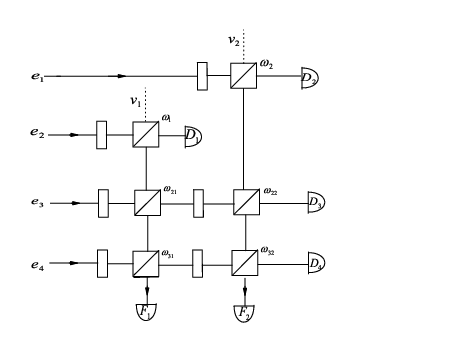
with ∑i=12Pi=∑j=34Pj=1\sum_{i=1}^{2}P_{i}=\sum_{j=3}^{4}P_{j}=1, each ρi\rho_{i} with it’s a​𝑝𝑟𝑖𝑜𝑟𝑖{\sl a~priori} probability to be λi\lambda_{i}, and ∑i=12λi=1\sum_{i=1}^{2}\lambda_{i}=1. Letting ηi=λ1⋅Pi\eta_{i}=\lambda_{1}\cdot P_{i} for i=1,2, and ηj=λ2⋅Pj\eta_{j}=\lambda_{2}\cdot P_{j} for j=3, 4, the above question can also be viewed as an operation on G≡{|Ψk>}G\equiv\{|\Psi_{k}>\} with ηk\eta_{k} as it probability for k=1, 2, 3, 4, we are required to tell if a state |Ψ?>∈G|\Psi_{?}>\in G belongs to G1≡{|Ψ1>,|Ψ2>}G_{1}\equiv\{|\Psi_{1}>,|\Psi_{2}>\} or G2≡{|Ψ3>,|Ψ4>}G_{2}\equiv\{|\Psi_{3}>,|\Psi_{4}>\} while there is a non-vanishing probability for fail. In terms of POVMs, E1|ψj>=E2|Ψi>=0E_{1}|\psi_{j}>=E_{2}|\Psi_{i}>=0 holds for |Ψj>∈G2|\Psi_{j}>\in G_{2} and |Ψi>∈G1|\Psi_{i}>\in G_{1}, respectively. Certainly, there is E0=Ie−∑k=12EkE_{0}=\textbf{I}^{e}-\sum_{k=1}^{2}E_{k}. The OPI in Fig.8 is designed to realize the unitary transformation in the way like

U⁡(ω)=R⁡(2)​R​(1),U(\omega)=R(2)R(1), (6.2)

where R(1) is the unitary transformation for filtering |Ψ2>|\Psi_{2}> from the rest of the states in G, R(2) is used to filter |Ψ′1>|\Psi^{\prime}_{1}> from |Ψ′3>|\Psi^{\prime}_{3}> and |Ψ′4>|\Psi^{\prime}_{4}>, whose definitions shall be given later. It should be noted that, when the detector D1D_{1} fired, we can not tell whether this signal is from |Ψ1>|\Psi_{1}> or |Ψ2>|\Psi_{2}> since the fact that these two states may have non-zero coefficients, c12c_{12} and c22c_{22}, along the rail e2e_{2}, respectively. It is certain that this signal can not come from the states, |Ψ3>|\Psi_{3}> and |Ψ4>|\Psi_{4}>, according to our discussion of DTR. One may compare the present R⁡(1)|Ψj>R(1)|\Psi_{j}>, with the one in discriminating three pure states,

R⁡(1)|Ψ2>\displaystyle R(1)|\Psi_{2}> =\displaystyle= d21|D1>+f21|F1>,\displaystyle d_{21}|D_{1}>+f_{21}|F_{1}>,
R⁡(1)|Ψ1>\displaystyle R(1)|\Psi_{1}> =\displaystyle= 1−|f11|2−|d11|2|Ψ1′>\displaystyle\sqrt{1-|f_{11}|^{2}-|d_{11}|^{2}}|\Psi^{\prime}_{1}> (6.3)
+d11|D1>+f11|F1>,\displaystyle+d_{11}|D_{1}>+f_{11}|F_{1}>,
R⁡(1)|Ψk>\displaystyle R(1)|\Psi_{k}> =\displaystyle= 1−|fk​1|2|Ψk′>+fk​1|F1>,\displaystyle\sqrt{1-|f_{k1}|^{2}}|\Psi^{\prime}_{k}>+f_{k1}|F_{1}>,

for k=3,4. Defining a Hilbert space H’ with it’s basis as {|ω21,r>,|ω31,r>,|e1>}\{|\omega_{21},r>,|\omega_{31},r>,|e_{1}>\}, there are three states:

|Ψ′1>\displaystyle|\Psi^{\prime}_{1}> =\displaystyle= c111−|f11|2−|d11|2|e1>\displaystyle\frac{c_{11}}{\sqrt{1-|f_{11}|^{2}-|d_{11}|^{2}}}|e_{1}>
+o31′−o34′​o41′1−|o43′|2|ω21,r>+o41′|Ψ4′>\displaystyle+\frac{o^{\prime}_{31}-o^{\prime}_{34}o^{\prime}_{41}}{\sqrt{1-|o^{\prime}_{43}|^{2}}}|\omega_{21},r>+o^{\prime}_{41}|\Psi^{\prime}_{4}>
|Ψ′3>\displaystyle|\Psi^{\prime}_{3}> =\displaystyle= 1−|o43′|2|ω21,r>+o43′|Ψ4′>,\displaystyle\sqrt{1-|o^{\prime}_{43}|^{2}}|\omega_{21},r>+o^{\prime}_{43}|\Psi^{\prime}_{4}>, (6.4)
|Ψ′4>\displaystyle|\Psi^{\prime}_{4}> =\displaystyle= ei​ϕ4′|ω31,r>,\displaystyle e^{i\phi^{\prime}_{4}}|\omega_{31},r>,

with oi​j′=<Ψi′|Ψj′>o^{\prime}_{ij}=<\Psi^{\prime}_{i}|\Psi^{\prime}_{j}>, these overlaps can be derived from Eq.(6.3) by the requirement that the oi​jo_{ij} keeps unchanged when the unitary transformation is performed on the input,

o1​k′=o1​k−f11∗​fk​1(1−|f11|2−|d11|2)​(1−|fk​1|2),o^{\prime}_{1k}=\frac{o_{1k}-f^{*}_{11}f_{k1}}{\sqrt{(1-|f_{11}|^{2}-|d_{11}|^{2})(1-|f_{k1}|^{2})}}, (6.5)

for k=3,4, while

o34′=o34−f31∗​f41(1−|f31|2)​(1−|f41|2).o^{\prime}_{34}=\frac{o_{34}-f_{31}^{*}f_{41}}{\sqrt{(1-|f_{31}|^{2})(1-|f_{41}|^{2})}}. (6.6)

In principle, we could realize R(2) as the filtering for N=3,

R⁡(2)|Ψ1′>\displaystyle R(2)|\Psi^{\prime}_{1}> =\displaystyle= d12|D1>+f12|F2>(1−|f11|2−|d11|2),\displaystyle\frac{d_{12}|D_{1}>+f_{12}|F_{2}>}{\sqrt{(1-|f_{11}|^{2}-|d_{11}|^{2})}},
R⁡(2)|Ψk′>\displaystyle R(2)|\Psi^{\prime}_{k}> =\displaystyle= ∑l=34dk​l|Dl>+fk​2|F2>1−|fk​1|2.\displaystyle\frac{\sum_{l=3}^{4}d_{kl}|D_{l}>+f_{k2}|F_{2}>}{\sqrt{1-|f_{k1}|^{2}}}. (6.7)

In the first run of filtering, the average value of failure is defined by

F1​(ω)=∑j=1N=4ηj​|fj​1|2,F_{1}(\omega)=\sum_{j=1}^{N=4}\eta_{j}|f_{j1}|^{2}, (6.8)

while the one for the second run of filtering is

F2​(ω)\displaystyle F_{2}(\omega) =\displaystyle= η1′​(1−c11′​sin2⁡ω2)\displaystyle\eta_{1}^{\prime}(1-c_{11}^{\prime}\sin^{2}\omega_{2}) (6.9)
+∑k=34ηk′​|o1​k′|21−c11′​sin2⁡ω2,\displaystyle+\frac{\sum_{k=3}^{4}\eta_{k}^{\prime}|o^{\prime}_{1k}|^{2}}{1-c_{11}^{\prime}\sin^{2}\omega_{2}},

in a standard form of filtering with N=3, and their a​𝑝𝑟𝑖𝑜𝑟𝑖{\sl a~priori} probability is

η1′=η1​(1−|f11|2−|d11|2),\displaystyle\eta^{\prime}_{1}=\eta_{1}(1-|f_{11}|^{2}-|d_{11}|^{2}),
ηk′=ηk​(1−|fk​1|2),\displaystyle\eta^{\prime}_{k}=\eta_{k}(1-|f_{k1}|^{2}), (6.10)

for k=3, 4, respectively. The coefficient, c11′c_{11}^{\prime}, may be read from Eq.(6.4) as

c11′=c11(1−|f11|2−|d11|2).c_{11}^{\prime}=\frac{c_{11}}{\sqrt{(1-|f_{11}|^{2}-|d_{11}|^{2})}}. (6.11)
Refer to caption
Figure 8: The OPI for discriminating two mixtures

VI.2 the POVMs realized by the OPI in Fig.8

As we have shown, it’s possible for us to get a U⁡(ω)U(\omega) which transforms each |Ψj>|\Psi_{j}> in the out-space:

|Ψ2>o​u​t\displaystyle|\Psi_{2}>^{out} =\displaystyle= d21|D1>+f21|F1>,\displaystyle d_{21}|D_{1}>+f_{21}|F_{1}>,
|Ψ1>o​u​t\displaystyle|\Psi_{1}>^{out} =\displaystyle= ∑j=12d1​j|Dj>+∑i=12f1​i|F1​i>,\displaystyle\sum_{j=1}^{2}d_{1j}|D_{j}>+\sum_{i=1}^{2}f_{1i}|F_{1i}>, (6.12)
|Ψk>o​u​t\displaystyle|\Psi_{k}>^{out} =\displaystyle= ∑l=34dk​l|Dl>+∑i=12fk​i|Fi>.\displaystyle\sum_{l=3}^{4}d_{kl}|D_{l}>+\sum_{i=1}^{2}f_{ki}|F_{i}>.

Using these expressions and the inverse R−1​(1)​R−1​(2)R^{-1}(1)R^{-1}(2), we can get

|D1>e\displaystyle|D_{1}>^{e} =\displaystyle= −sin⁡ω1|e2>,\displaystyle-\sin\omega_{1}|e_{2}>,
|F1>e\displaystyle|F_{1}>^{e} =\displaystyle= (Ie−|D1>e<D1|)|Ψ2>1−|d21|2,\displaystyle\frac{(\textbf{I}^{e}-|D_{1}>^{e}<D_{1}|)|\Psi_{2}>}{\sqrt{1-|d_{21}|^{2}}},
|D2>e\displaystyle|D_{2}>^{e} =\displaystyle= −sin⁡ω2|e1>,\displaystyle-\sin\omega_{2}|e_{1}>, (6.13)
|F2>e\displaystyle|F_{2}>^{e} =\displaystyle= (Ie−∑i=12|Di>e<Di|−|F1>e<F1|)|Ψ1>OPEN1−|f11|2−∑i=12|d1​i|2)\displaystyle\frac{(\textbf{I}^{e}-\sum_{i=1}^{2}|D_{i}>^{e}<D_{i}|-|F_{1}>^{e}<F_{1}|)|\Psi_{1}>}{\sqrt{1-|f_{11}|^{2}-\sum_{i=1}^{2}|d_{1i}|^{2})}}

with di​j=<Dj|Ψi>d_{ij}=<D_{j}|\Psi_{i}> and fi​j=<Fj|Ψi>f_{ij}=<F_{j}|\Psi_{i}>, the POVMs are defined by

E1\displaystyle E_{1} =\displaystyle= ∑i=12|Di>e<Di|,\displaystyle\sum_{i=1}^{2}|D_{i}>^{e}<D_{i}|,
E0\displaystyle E_{0} =\displaystyle= ∑i=12|Fi>e<Fi|,\displaystyle\sum_{i=1}^{2}|F_{i}>^{e}<F_{i}|, (6.14)
E2\displaystyle E_{2} =\displaystyle= ∑j=34|Dj>e<Dj|=Ie−∑m=01Em,\displaystyle\sum_{j=3}^{4}|D_{j}>^{e}<D_{j}|=\textbf{I}^{e}-\sum_{m=0}^{1}E_{m},

With these operators in hands, we could define the average value of fail

F⁡(ω)=∑j=1N=4ηj​<Ψj|E0|Ψj>,F(\omega)=\sum_{j=1}^{N=4}\eta_{j}<\Psi_{j}|E_{0}|\Psi_{j}>, (6.15)

and one may check that

F⁡(ω)=F1​(ω)+F2​(ω).F(\omega)=F_{1}(\omega)+F_{2}(\omega). (6.16)

The coefficients, which are needed in the calculation of F⁡(ω)F(\omega), are list here

f11\displaystyle f_{11} =\displaystyle= o21−c12​c22​sin2⁡ω11−c222​sin2⁡ω1,\displaystyle\frac{o_{21}-c_{12}c_{22}\sin^{2}\omega_{1}}{\sqrt{1-c_{22}^{2}\sin^{2}\omega_{1}}},
f21\displaystyle f_{21} =\displaystyle= 1−c222​sin2⁡ω1,\displaystyle\sqrt{1-c_{22}^{2}\sin^{2}\omega_{1}},
fk​1\displaystyle f_{k1} =\displaystyle= o2​k1−c222​sin2⁡ω1,\displaystyle\frac{o_{2k}}{\sqrt{1-c_{22}^{2}\sin^{2}\omega_{1}}},
d11\displaystyle d_{11} =\displaystyle= −c12sinω1,\displaystyle-c_{12}\sin\omega_{1}, (6.17)
d12\displaystyle d_{12} =\displaystyle= −c11sinω2,\displaystyle-c_{11}\sin\omega_{2},
f12\displaystyle f_{12} =\displaystyle= 1−∑i=12|d1​i|2−|f11|2,\displaystyle\sqrt{1-\sum_{i=1}^{2}|d_{1i}|^{2}-|f_{11}|^{2}},
fk​2\displaystyle f_{k2} =\displaystyle= o1​k−f11∗​fk​11−∑i=12|d1​i|2−|f11|2,\displaystyle\frac{o_{1k}-f^{*}_{11}f_{k1}}{\sqrt{1-\sum_{i=1}^{2}|d_{1i}|^{2}-|f_{11}|^{2}}},

with k=3, 4.

Refer to caption
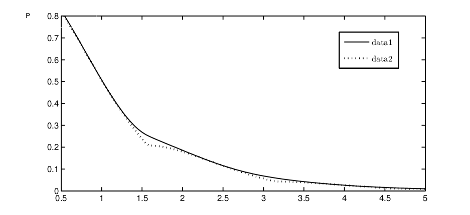
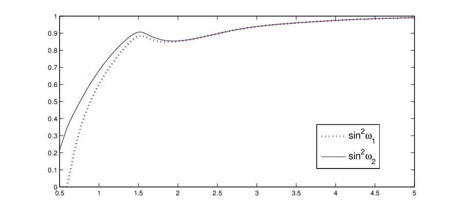
Figure 9: the optimal results of Fo​p​tF^{opt} in Eq.(6.16), the present results are described by the solid line, while the analytical results in dash line.
Refer to caption
Figure 10: the optimal choice of ω\omega

VI.3 an application of the POVMs

In a recent work, Raynal 𝑒𝑡​𝑎𝑙.{\sl et~al.} considered the question, which came from the implementation of the BB84 by using the four quantum optical coherent states {|±α>\{|\pm\alpha>,|±iα>}|\pm i\alpha>\} [35], of how to discriminate the following two mixtures:

ρ1\displaystyle\rho_{1} =\displaystyle= 12(|α><α|+|−α><−α|),\displaystyle\frac{1}{2}(|\alpha><\alpha|+|-\alpha><-\alpha|),
ρ2\displaystyle\rho_{2} =\displaystyle= 12(|iα><iα|+|−iα><−iα|),\displaystyle\frac{1}{2}(|i\alpha><i\alpha|+|-i\alpha><-i\alpha|), (6.18)

and the authors expressed the optimal failure probability in terms of the mean photon number:

Fo​p​t=e−μ​(|cos⁡μ|+|sin⁡μ|),F^{opt}=e^{-\mu}(|\cos\mu|+|\sin\mu|), (6.19)

with μ≡|α|2\mu\equiv|\alpha|^{2}.

Here, we shall reconsider this problem with the POVMs in Eqs.(13-14). Writing the all the known parameters in terms of α\alpha, we designed a program to get the optimal velue of F⁡(ω)F(\omega) in Eq.(6.15) by scanning in the parameters space 0≤ω1,ω2≤2​π.0\leq\omega_{1},\omega_{2}\leq 2\pi. The final result of our calculation and the analytic solution in Eq.(6.19) are both presented in Fig.9, while the optimal values of the ω1\omega_{1} and ω2\omega_{2} are given in Fig.10. Although in some regions of Fig.9, small discrepancy still exists, our numerical calculations are consistent with the analytical solutions well in most parts of the parameter space, this fact shall give great supports to our present proposal.
Refer to caption
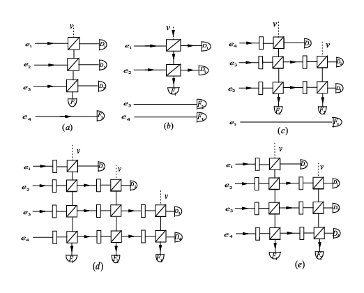
Figure 11: The OPIs for the following cases: (a) filtering |Ψ1>|\Psi_{1}> from |Ψ2>|\Psi_{2}> and |Ψ3>|\Psi_{3}> with |Ψ4>|\Psi_{4}> as the background; (b) filtering |Ψ1>|\Psi_{1}> from |Ψ2>|\Psi_{2}> with |Ψ3>|\Psi_{3}> and |Ψ4>|\Psi_{4}> as the background; (c) discriminating three pure states with |Ψ4>|\Psi_{4}> as the background; (d) discriminating four pure states and (e) discriminating |Ψ1>|\Psi_{1}>, |Ψ2>|\Psi_{2}> and {|Ψ3>,|Ψ4>}\{|\Psi_{3}>,|\Psi_{4}>\}.

VII discussion

In the present paper, we always adopt a naive understanding of the mixture: suppose a mixtures is denoted by ρ\rho, for examples, ρ=∑j=1Nηj|Ψj><Ψj|\rho=\sum_{j=1}^{N}\eta_{j}|\Psi_{j}><\Psi_{j}|, in each run of the experiment, the input for our OPI is still a pure state belonging to the set {|Ψj>}\{|\Psi_{j}>\}.

For the system of N=2 and N=3, we have given a series of derivations to show why these cases can be solved by applying the argument of filtering, certainly, within the DTR. The case discussed in Sec.VI, is an important case of N=4. There are still others types of operations for N=4 system: (a) filtering |Ψ1>|\Psi_{1}> from |Ψ2>|\Psi_{2}> and |Ψ3>|\Psi_{3}> with |Ψ4>|\Psi_{4}> as the background; (b) filtering |Ψ1>|\Psi_{1}> from |Ψ2>|\Psi_{2}> with |Ψ3>|\Psi_{3}> and |Ψ4>|\Psi_{4}> as the background; (c) discriminating three pure states with |Ψ4>|\Psi_{4}> as the background; (d) discriminating four pure states and (e) discriminating |Ψ1>|\Psi_{1}>, |Ψ2>|\Psi_{2}> and {|Ψ3>,|Ψ4>}\{|\Psi_{3}>,|\Psi_{4}>\}. Their OPIs are given in Fig.11. In principle, all these cases can be solved by reducing to filtering. For the cases where more than once filtering is needed, it’s hard for us to find analytical solutions for the optical values.

A important profit of our scheme should be mentioned here: the POVMs for each case shall be able to, although maybe not in a optimal way, complete the task of discriminating when the a priori probability of each state is not completely decided.

In end of this paper, we would like to emphasize that : first, for a given case, if one could prepare the input in the one-photon state, then our OPI can be directly used for the optical experimental realization. Then, although the POVMs are from the one-photon picture, yet they are are general and state-type independent. Finally, a proposal, rather than a complete proof, has been given here in order to find a solution to the problem of the quantum state unambiguous discrimination. It’s still a open question that: whether the task of quantum state unambiguous discriminating, either of pure states or of mixtures, can be solved by reducing it to the problem of quantum state filtering?

Acknowledgements.
We wish to acknowledge the helpful discussion of Prof. Chen L.X.

*

Appendix A some known matrices for the low-dimensional cases.

For N=2,

O⁡(2)=(1o12o211),O(2)=\left(\begin{array}[]{cc}1&o_{12}\\ o_{21}&1\\ \end{array}\right), (1.1)
O⊥​(2)=(1−o12−o211),O^{\bot}(2)=\left(\begin{array}[]{cc}1&-o_{12}\\ -o_{21}&1\\ \end{array}\right), (1.2)

with

det(O−1​(2))=1−|o12|2,t1=t2=1−|o12|2\det(O^{-1}(2))=1-|o_{12}|^{2},~~t_{1}=t_{2}=\sqrt{1-|o_{12}|^{2}} (1.3)

For N=3,

O⁡(3)=(1o12o13o211o23o31o321),O(3)=\left(\begin{array}[]{ccc}1&o_{12}&o_{13}\\ o_{21}&1&o_{23}\\ o_{31}&o_{32}&1\\ \end{array}\right), (1.4)

with A(3), the adjoint of O(3), to be

(1−|o23|2o13​o32−o12o12​o23−o13o23​o31−o211−|o13|2o21​o13−o23o32​o21−o31o31​o12−o321−|o12|2,)\left(\begin{array}[]{ccc}1-|o_{23}|^{2}&o_{13}o_{32}-o_{12}&o_{12}o_{23}-o_{13}\\ o_{23}o_{31}-o_{21}&1-|o_{13}|^{2}&o_{21}o_{13}-o_{23}\\ o_{32}o_{21}-o_{31}&o_{31}o_{12}-o_{32}&1-|o_{12}|^{2}\\ \end{array},\right) (1.5)

The inverse O−1​(3)O_{-1}(3) could be given by O−1​(3)=A~​(3)/det(O)O_{-1}(3)=\tilde{A}(3)/\det(O) with

det(O⁡(3))=\displaystyle\det(O(3))= 1−|o12|2−|o13|2−|o23|2\displaystyle 1-|o_{12}|^{2}-|o_{13}|^{2}-|o_{23}|^{2} (1.6)
+o12​o23​o31+o21​o13​o32\displaystyle+o_{12}o_{23}o_{31}+o_{21}o_{13}o_{32}

which has applications in

t1=det(O)1−|o23|2,t2=det(O)1−|o13|2,t3=det(O)1−|o21|2.t_{1}=\sqrt{\frac{\det(O)}{1-|o_{23}|^{2}}},\\ t_{2}=\sqrt{\frac{\det(O)}{1-|o_{13}|^{2}}},\\ t_{3}=\sqrt{\frac{\det(O)}{1-|o_{21}|^{2}}}. (1.7)

The overlap matrix , O⊥​(3)O^{\bot}(3), is known with the form:

O⊥(3)=(1o13​o32−o12(1−|o23|2)​(1−|o13|2)o12​o23−o13(1−|o23|2)​(1−|o12)o23​o31−o21(1−|o23|2)​(1−|o13|2)1o21​o13−o23(1−|o13|2)​(1−|o12|2)o32​o21−o31(1−|o23|2)​(1−|o12|2)o31​o12−o32(1−|o13|2)​(1−|o12|2)1,)O^{\bot}(3)=\left(\begin{array}[]{ccc}1&\frac{o_{13}o_{32}-o_{12}}{\sqrt{(1-|o_{23}|^{2})(1-|o_{13}|^{2})}}&\frac{o_{12}o_{23}-o_{13}}{\sqrt{(1-|o_{23}|^{2})(1-|o_{12})}}\\ \frac{o_{23}o_{31}-o_{21}}{\sqrt{(1-|o_{23}|^{2})(1-|o_{13}|^{2})}}&1&\frac{o_{21}o_{13}-o_{23}}{\sqrt{(1-|o_{13}|^{2})(1-|o_{12}|^{2})}}\\ \frac{o_{32}o_{21}-o_{31}}{\sqrt{(1-|o_{23}|^{2})(1-|o_{12}|^{2})}}&\frac{o_{31}o_{12}-o_{32}}{\sqrt{(1-|o_{13}|^{2})(1-|o_{12}|^{2})}}&1\\ \end{array},\right) (1.8)

References

  • [1] D. Dieks, Phys.Lett.A 126,303(1998).
  • [2] I. D. Ivanovic, Phys.Lett.A 123, 257(1987).
  • [3] A. Peres, Phys.Lett.A 128, 19(1998).
  • [4] G. Jaeger and A. Shimony, Phys.Lett.A 197, 83(1995).
  • [5] A. Chefles, Phys.Lett.A 239, 339(1998).
  • [6] A. Peres and D. R. Terno, J.Phys.A 31,7105(1998).
  • [7] L. M. Duan and G. C. Guo, Phys.Rev.Lett. 80, 4999(1998).
  • [8] Y. Sun, M. Hillery and J. A. Bergou, Phys. Rev. A 𝟔𝟒\mathbf{64}, 022311 (2001).
  • [9] A. Chefles and S. M. Barnett, Phys.Lett.A 250, 223(1998).
  • [10] O. Jiménez, X. Sánchez-Lozano, E. Burgos-Inostroza, A. Delgado and C. Saavedra, Phy.Rev.A 76, 062107(2007).
  • [11] M. A. Jafarizadeh, M. Rezaei, N. Karimi and A. R. Amiri, Phys.Rev.A 77, 042314(2008).
  • [12] S. Zhang and M. Ying, Phys.Rev.A 65, 062322(2002).
  • [13] Y. C. Eldar, M. Stojic, and B. Hassibi, Phys.Rev.A 69, 062318(2004).
  • [14] Ph. Raynal, N. Lütkenhaus and S. J. Van Enk, Phys.Rev.A 68, 022308(2004).
  • [15] Ph. Raynal and N. Lütkenhaus, Phys.Rev.A, 052322(2007).
  • [16] T. Rudolph, R. W. Speckkens and P. S. Turner, Phys.Rev.A 68, 022308(2003).
  • [17] Y. Feng, R. Duan and M. Ying, Phys.Rev.A 70, 012308(2004).
  • [18] U. Herzog and J. A. Bergou, Phys.Rev.A 71, 050301(R)(2005).
  • [19] Ph. Raynal and N. lutkenhaus, Phys.Rev.A 72, 022342(2005).
  • [20] X. F. zhou, Y. S. Zhang and G. C. Guo, Phys.Rev.A 75, 052314(2007).
  • [21] J. A. Bergou, U. Herzog and M. Hikkery, Phys.Rev.Lett. 90, 257901(2003).
  • [22] J. A. Bergou, U. Herzog and M. Hillery, Phys.Rev.A 71, 042314(2005).
  • [23] 23) Y. Sun, J. A. Bergou and M. Hillery, Phys.Rev.A 66, 02315(2002).
  • [24] J. A. Bergou, E. Feldman and M. Hillery, Phys.Rev.A 66, 02315 (2006).
  • [25] U. Herzog, Phys.Rev.A 75, 052309(2007).
  • [26] S. M. Barnett, A. Chefles and I. Jex, Phys.Lett.A 307,189(2003).
  • [27] M. Kleinmann, H. Kampermann and D. Bruß, Phys.Rev.A 72, 032308(2005).
  • [28] J. A. Bergou and M. Hillery, Phys. Rev. Lett. 𝟗𝟒\mathbf{94}, 160501 (2005).
  • [29] J. A. Bergou, V. Buzek, E. Feldman, U. Herzog, and M. Hillery, Phys. Rev. A 𝟕​3{\mathbf{7}3}, 062334 (2006).
  • [30] A. Hayashi, M. Horibe, and T. Hashimoto, Phys. Rev. A 𝟕𝟑\mathbf{73}, 012328 (2006).
  • [31] K.Kraus, States,Effects and operations:Fundamental Notions of Quantum Theory (Springer, Berlin 1983).
  • [32] M. A. Neumark, Izv. Akal. Nauk SSSR. Ser. Mat. 𝟒\mathbf{4}, 277 (1940).
  • [33] B. Kolman and D. R. Hiu, Introductory Linear Algebra( Prentice Hall, Upper Saddle River, New Jersey 07458).
  • [34] M. Reck, A. Zeilinger, H.J. Bernstein and P. Bertani, Phys. Rev. Lett. 𝟕𝟑\mathbf{73}, 58 (1994).
  • [35] C. H. Bennett and G. Brassard, Proceedings of IEEE International Conference on Computers, Systems and Signal Processing, Bangalore, India(IEEE,New York, 1984).