Experimental Consequences of the S-wave $\cos(k_{x})\cdot\cos(k_{y})$ Superconductivity in the Iron-Pnictides

The recent discovery of iron-based superconductors with a transition temperature as high as 55K has stimulated a flurry of experimental and theoretical activity [2, 3, 4, 5, 6, 7, 8, 9, 10, 11]. However, a conclusive observation of the pairing symmetry still remains elusive, with both nodal and nodeless order parameters reported in experimental observations.

Numerical and analytic research suggests that the antiferromagnetic exchange coupling between Fe sites is strong [12, 13, 14]. Owing to As-mediated hopping, antiferromagnetic exchange exists not only between the nearest neighbor (NN) Fe sites, but also between next nearest neighbor (NNN) sites. Moreover, the NNN coupling strength $J_{2}$ is stronger than the NN coupling strength $J_{1}$. The $J_{1}-J_{2}$ model produces half-filled magnetic physics consistent with experimental neutron data [15]. A nematic magnetic phase transition has been predicted in this model [16, 17], consistent with the experimental observation of a structural transition preceding the spin density wave (SDW) formation. This model suffers, however, from an important deficiency - it is an insulator whereas the real material is an, albeit bad, metal. We, however, believe that the spin-spin interaction insight is important to the physics of the iron-pnictides.

In a recent paper [1], two of us added electron itineracy to the problem and studied a $t-J_{1}-J_{2}$ model without band renormalization. We found that the singlet-forming $J_{1}-J_{2}$ interaction gives rise to four possible pairing symmetries: $\cos(k_{x})\pm\cos(k_{y})$, $\sin(k_{x})\cdot\sin(k_{y})$ and $\cos(k_{x})\cdot\cos(k_{y})$. The last two are strongly preferred from an interaction standpoint when $J_{2}>J_{1}$, but only $\cos(k_{x})\cdot\cos(k_{y})$ matches the symmetry of the iron-pnictide Fermi surface: it is maximal around $(0,0),(\pi,0),(0,\pi),(\pi,\pi)$ - the location of the Fermi surfaces in the unfolded one-iron per site Brilloiun zone. Although we used a specific, two band model for our calculation [1], our results are completely independent of any model, as long as the dominating interaction is next-nearest neighbor $J_{2}$ and the Fermi surfaces are located close to the aforementioned spots in the Brillouin zone. Some order parameters (such as $d_{xy}=\sin(k_{x})\cdot\sin(k_{y})$ and others) mismatch the Fermi surface symmetry and can be discarded. We note that $\cos(k_{x})\cdot\cos(k_{y})$ changes sign between the electron and hole pockets in the Brillouin zone. In this sense, it resembles the order parameter proposed by Mazin through weak-coupling general arguments [18]. At moderate doping, our gap is isotropic within the same Fermi surface, while changing sign between electrons and hole pockets, but at relatively high doping $\cos(k_{x})\cdot\cos(k_{y})$ exhibits some anisotropy even within the same Fermi surface.

Neutron measurements have found antiferromagnetic stripe order of Fe moments ranging from $0.26\mu_{B}$ in NaOFeAs[19] and $0.36\mu_{B}$[20] in LaOFeAs to $0.8\mu_{B}$ in CeOFeAs[21] and SrFe₂As₂ [22]. A magnetic moment of $0.8\mu_{B}$ is fully consistent with a purely localized spin-one Heisenberg model. While a magnetic moment of $0.3\mu_{B}$ is smaller than what is expected in a purely localized spin-one system, it is rather larger than what can be obtained in a truly weak coupling theory. We point out that, due to imperfect nesting, weak coupling theory requires large values of $U/t\sim 4$ to explain even small magnetic moments ($<0.2\mu_{B}$), clearly outside the weak-coupling limit [23]. Considering these facts, together with the rather high resistivity of the iron-pnictides, we find that the experimental evidence paints a picture of the iron-pnictides as being at moderate interaction couplings. Thus, moderate to strong coupling models can provide an accurate qualitative description of the observed phenomena. In fact, the $t-J_{1}-J_{2}$ model predicts the right physics of the parent state SDW as well as the $\cos(k_{x})\cdot\cos(k_{y})$ order parameter.

In this paper we focus on the experimental properties of several superconducting order parameters proposed in the iron-pnictides, with particular emphasis on the $\cos(k_{x})\cdot\cos(k_{y})$ order parameter. We look at a simplified two-band superconducting model and obtain the spectral function, density of states, tunneling differential conductance, penetration depth and NMR spin relaxation time. We stress the important point that the $\cos(k_{x})\cdot\cos(k_{y})$ order parameter features lines of zeroes at $(\pm\pi/2,k_{y})$ and $(k_{x},\pm\pi/2)$, as in Fig. 1 (obviously, irrespective of its harmonic form, any order parameter changing sign between the electron and hole Fermi surfaces must have zero-lines). Thus, at low doping, the hole and electron Fermi pockets are far away from the zero lines of the order parameter and the superconductivity is nodeless.

Close to half-filling, we find that the $\cos(k_{x})\cdot\cos(k_{y})$ order parameter exhibits an exponentially decaying $\delta\lambda(T)=\lambda(T)-\lambda(0)$, where $\lambda(T)$ is the penetration depth at temperature $T$, as expected for a nodeless superconductor. However, upon doping, the gap on the Fermi surface varies in magnitude: for electron doping, the gap decreases on the electron pocket and increases on the hole pocket. The penetration depth is sensitive to the smallest gap in the system, and hence exhibits a weakened exponential decay upon doping. This could explain the conflicting values of the gap parameters obtained by fitting the penetration depth experiments to the BCS exponential form [24, 25, 26]. In the unlikely event that the system remains superconducting at very large doping, then the Fermi surfaces will cross the line of zeros of $\cos(k_{x})\cdot\cos(k_{y})$ at around $35\%$ doping, and cause $\delta\lambda(T)$ to become linearly dependent on T.

We also calculate the NMR spin relaxation rate $1/T_{1}$ of the bare superconductor and find that it factorizes into inter- and intra-band contributions. While, for the $\cos(k_{x})\cdot\cos(k_{y})$ order parameter, the inter-band contribution to the NMR spin relaxation rate does not exhibit a coherence peak, the intra-band contribution is larger than the inter-band contribution and still exhibits an enhancement right below $T_{c}$ owing to its fully gapped $s$-wave nature. Adding the two contributions we find that, although the coherence peak for $\cos(k_{x})\cdot\cos(k_{y})$ is smaller than for a sign-preserving gap such as, for example, $|\cos(k_{x})\cdot\cos(k_{y})|$, it is still present due to the intra-band contribution. The coherence peak can be strongly reduced if the intra-band scattering is stronger than inter-band scattering or if the samples are strongly disordered. If the As structure factor $A({\mathbf{q}})$ is taken into account, the inter-band contribution is severely reduced due to the fact that $A({\mathbf{q}})=\cos(q_{x}/2)\cos(q_{y}/2)$ is zero close to the wavevector difference between the electron and hole Fermi surfaces: ${\mathbf{q}}=(\pm\pi,0),(0,\pm\pi)$. The As structure factor also reduces the overall coherence peak by smearing the intra-band contribution.

We approximate the typical iron-based material by a two-dimensional square lattice of Fe atoms, since the superconductivity has been shown to be associated with the FeAs layer. To capture the degeneracy of the $d_{xz}$ and $d_{yz}$ orbitals on the Fe atoms, we use the two-orbital per site model proposed by Ref. 23. Although this description is only valid in the case of an unphysically large crystal field splitting, we particularize to this model for analytic simplicity. The kinetic part of the Hamiltonian is written:

Here, $\psi^{\dagger}_{{\mathbf{k}}\sigma}=(c_{1,{\mathbf{k}},\sigma}^{\dagger},c_{2,{\mathbf{k}},\sigma}^{\dagger})$ is the creation operator for spin $\sigma$ electrons in the two orbitals $(1,2)=(d_{xz},d_{yz})$, $\mu$ is the chemical potential, and the matrix elements are

While Eq. (Model –) is only a simplified version of the true band structure of the material, it produces Fermi pockets that resemble those predicted by density functional theory (see Fig. 1). The eigenvalues of (Model –) are:

where $\epsilon_{\pm}=(\epsilon_{x}\pm\epsilon_{y})/2$. In the following, we take $t_{1}=-1$, $t_{2}=1.3$, and $t_{3}=t_{4}=-0.85$. The undoped compound, where there are two electrons per site, corresponds to $\mu=1.54$.

We now assume that the interacting part of the Hamiltonian induces singlet pairing between electrons within each orbital, but we make no further assumptions about the form of the interaction or the pairing mechanism. Then we introduce pairing gaps $\Delta_{1,2}$ for each orbital and we write down the mean-field effective Hamiltonian $H(\Delta_{1},\Delta_{2})=\sum_{\mathbf{k}}\Psi({\mathbf{k}})^{\dagger}B({\mathbf{k}})\Psi({\mathbf{k}})$, where

with $\xi_{x}=\epsilon_{x}-\mu$, $\xi_{y}=\epsilon_{y}-\mu$, and we have used the four-component spinor $\Psi({\mathbf{k}})=(c_{1,{\mathbf{k}},\uparrow},c_{1,-{\mathbf{k}},\downarrow}^{\dagger},c_{2,{\mathbf{k}},\uparrow},c_{2,-{\mathbf{k}},\downarrow}^{\dagger})$. We neglect inter-orbital pairing in order to make the problem analytically tractable. This is also reasonable because two of us proved in Ref. 1 that, at least for the case of the $t-J_{1}-J_{2}$ model (and hence for the most important gap we will be focusing on - $\cos(k_{x})\cdot\cos(k_{y})$), the inter-orbital pairing expectation value is negligible even in the case of strong Hund’s rule coupling.

The symmetry of the superconducting order parameter $\Delta({\mathbf{k}})$ has two possible $d$-wave types [1]: $d_{x^{2}-y^{2}}\sim\Delta_{0}(\cos k_{x}-\cos k_{y})$ and $d_{xy}\sim\Delta_{0}\sin k_{x}\sin k_{y}$, and three possible $s$-wave types [1]: $s_{x^{2}+y^{2}}\sim\Delta_{0}(\cos k_{x}+\cos k_{y})$, $s_{x^{2}y^{2}}\sim\Delta_{0}\cos k_{x}\cos k_{y}$, as well as the constant gap ($s_{0}$) which is not allowed in the $t-J_{1}-J_{2}$ model but can obviously appear in other interacting models. The $C_{4}$ symmetry of the underlying lattice maps $k_{x}\leftrightarrow k_{y}$ and $d_{xz}\leftrightarrow d_{yz}$. Hence for all the pairing symmetries described above we have $\Delta_{1}(k_{x},k_{y})=\Delta_{2}(k_{y},k_{x})$, except for $d_{x^{2}-y^{2}}$ where $\Delta_{1}(k_{x},k_{y})=-\Delta_{2}(k_{x},k_{y})$. [1] The $d_{x^{2}-y^{2}}$, $d_{xy}$ and $s_{x^{2}+y^{2}}$ pairing symmetries are nodal while the other pairing symmetries are nodeless. We now proceed to analyzing the experimental consequences of these pairing symmetries.

The single-particle density of states (DOS) can be written as:

where $\mathcal{A}({\mathbf{k}},\omega)$ is the spectral function and $\mathcal{G}_{11}({\mathbf{k}},\omega+i\delta)$ and $\mathcal{G}_{33}({\mathbf{k}},\omega+i\delta)$ are the electron components of the superconducting Green’s function. Generally, we find:

where $E_{1}$ and $E_{3}$ are the positive eigenvalues of the matrix $B({\mathbf{k}})$ in (5) (see Ref. 1). For the case where $\Delta_{1}=\Delta_{2}=\Delta$ (valid except for the $d_{x^{2}-y^{2}}$ pairing symmetry), we have the simplified form:

with $E_{\pm}^{\Delta}({\mathbf{k}})=\sqrt{E_{\pm}^{2}({\mathbf{k}})+\Delta^{2}({\mathbf{k}})}$. This resembles two independent single-band superconductors with the energy dispersions $E_{\pm}$.

The spectral function at the Fermi energy $\mathcal{A}({\mathbf{k}},\omega=0)$ contains information about the nodal structure for each pairing symmetry, as shown in Fig. 2. The $s_{x^{2}+y^{2}}$ pairing symmetry exhibits nodes on the Fermi surface for all dopings when $k_{x}=(\pm\pi-k_{y}),(\pm\pi+k_{y})$ and thus only the hole Fermi pockets are fully gapped. The $d_{xy}$ pairing symmetry also has nodes for all doping, but in this case they occur when $k_{x,y}=0,\pm\pi$ and so all of the Fermi surfaces are gapless. The $d_{x^{2}-y^{2}}$ pairing symmetry (not shown) exhibits nodes on the Fermi surface of the hole pockets for any doping and it has a similar effect on the electron pockets as the $s_{x^{2}y^{2}}$ pairing symmetry which is the dominant pairing symmetry that we found in Ref. 1. The $s_{x^{2}y^{2}}$ pairing only has nodes on the Fermi surface above a critical doping $\mu\simeq 2$ since the zeros of the gap lie at $k_{x,y}=\pm\pi/2$. For $\mu<2$, the electron Fermi surfaces are fully gapped, like the hole Fermi surfaces. In principle, information about the form of the $s_{x^{2}y^{2}}$ gap can be obtained through ARPES. In the folded Brillouin Zone, there are two hole pockets at the $\Gamma$ point. A $\cos(k_{x})\cdot\cos(k_{y})$ order parameter predicts a larger gap for the smaller hole Fermi surface and smaller gap for the larger hole Fermi surface.

Tunneling measurements access the local DOS to a first approximation. Specifically, if we assume that both the tunneling matrix element and the probe DOS are momentum independent, then the tunneling differential conductance is [27]:

where $eV$ is the bias voltage of the tunneling probe and $n^{\prime}_{F}(E)\equiv\partial n_{F}(E)/\partial E$ is the derivative of the Fermi function. In the limit of zero temperature, we obviously recover the DOS. From Fig. 3, we see that a fully-gapped Fermi surface yields a corresponding gap in $dI/dV$ at low energies, while for a gapless Fermi surface, the DOS grows quasi-linearly with energy at $\omega=0$, a text-book result. In particular, $s_{x^{2}+y^{2}}$ ($d_{x^{2}-y^{2}}$) pairing produces a four-peak structure in the differential conductance because in this case each band sees a different order parameter: the hole (electron) Fermi surfaces are fully gapped while the electron (hole) Fermi surfaces are gapless.

Focussing on $s_{x^{2}y^{2}}$ pairing[1] (Fig. 4), we find that the differential conductance smoothly evolves from fully gapped to gapless behavior with increasing doping, as expected. Moreover, when the doping is large, we obtain a four-peak structure similar to $s_{x^{2}+y^{2}}$ pairing, because we also have a fully-gapped hole Fermi surface and a partially-gapped electron Fermi surface. While it is likely that the material cannot be doped high enough so that the $s_{x^{2}y^{2}}=\cos(k_{x})\cdot\cos(k_{y})$ superconductor becomes gapless (the material will most likely exit the superconducting state at such high dopings), we believe that the predictions above, in particular the evolution of the differential conductance with doping, could be used in careful experiments to falsify this order parameter.

Measurements of the penetration depth in the Fe-based superconductors were the first to suggest that the Fermi surfaces are fully gapped [24, 26, 25]. The experiments show an exponentially temperature decay of $\delta\lambda(T)=\lambda(T)-\lambda(0)$. Among the different order parameters studied here, such a scenario is only consistent with $s_{x^{2}y^{2}}$ symmetry at low doping or a constant $s$-wave gap. We now obtain the penetration depth for the bare two band superconductor with generic $\Delta_{1,2}$ gaps.

To obtain the penetration depth, we perform a text-book exercise. We write the FeAs model in real space and introduce a gauge field via the Peierls substitution $c_{i,\alpha}^{\dagger}c_{j,\beta}\rightarrow c_{i,\alpha}^{\dagger}\exp(i\int_{i}^{j}\vec{A}\cdot d\vec{l})c_{j,\beta}$ where $\alpha,\beta$ are the two orbital indices. We pick a Landau gauge $\vec{A}=A\hat{x}$ and expand to second order in $A$, thus obtaining $H(A)$. The second order term in $A$ is the diamagnetic current while the first order term gives the paramagnetic current, whose response must be calculated in linear response. We have:

hence

Using translational invariance, the expectation value of the diamagnetic current in the ground state is:

where the expectation values of the above operators are computed in the appropriate ground state. The paramagnetic current is obtained through a correlation function in linear response: $j_{x}^{p}({\mathbf{q}},\omega)=Q_{xx}({\mathbf{q}},\omega)A_{x}({\mathbf{q}},\omega)$:

This is the vacuum polarization. For the FeAs metal (not the superconductor), this is explicitly given by:

where $\omega_{m}=(2m+1)\pi T$ is a fermionic Matsubara frequency while $\nu_{n}=2n\pi T$ is a bosonic one. $J_{x}$ is the current operator, which is expressed as $\partial{H}/\partial{k_{x}}$ in the metal. For the response to a magnetic field, the limit that has to be taken is, upon analytic continuation, $i\nu_{n}\rightarrow\omega+i\delta$, $\omega=0$, ${\mathbf{q}}\rightarrow 0$. The opposite limit $\omega\rightarrow 0$, ${\mathbf{q}}=0$ gives the response to an electric field, and hence the electrical conductivity. After tedious but straightforward algebra, we obtain for the FeAs metal:

The overall factor of $2$ reflects the spin multiplicity. Besides the usual paramagnetic expression (first two terms in Eq. (15)), the cross-orbital exchange introduces an extra second term. We have checked that this paramagnetic term completely cancels the diamagnetic ground state expectation value, as is required for a metal. We performed the same calculation in the superconductor. The charge matrix operator in our superconductor is:

The current operator uses only the kinetic part of the kinetic Hamiltonian and is obtained from the continuity equation, giving:

where $\{,\}$ is the anticommutator. The penetration depth $\delta\lambda(T)=\lambda(T)-\lambda(0)$ is proportional to the current-current correlation function which uses the Green’s function of the superconductor, not written here due to space restrictions. For the case where $\Delta_{1}=\Delta_{2}$, we can write the current-current correlation function as:

We see that the cross-orbital exchange introduces an extra term, similar to the case of the FeAs metal, but the largest contribution to the temperature dependence arises from the first term. We have obtained the expression of the current-current correlation function for general $\Delta_{1}\neq\Delta_{2}$, but we do not include it for space reasons.

We now plot the low temperature dependence of the penetration depth $\delta\lambda(T)=\lambda(T)-\lambda(0)$ for different superconducting gaps (see Fig. 5). As expected, the nodal order parameters exhibit a linear $T$ dependence (in the absence of impurities) while the nodeless order parameters exhibit an exponentially decaying penetration depth. However, as shown in Fig. 6, one qualitative feature is that the $\cos(k_{x})\cdot\cos(k_{y})$ order parameter exhibits, upon doping, a weakened exponential decay, a signature that the gap on the electron (hole) surface decreases upon electron (hole) doping. This is a direct consequence of the existence of a line of zeroes in between the electron and hole pockets. Above some critical doping, the exponential decay of $\delta\lambda(T)$ in the $\cos(k_{x})\cdot\cos(k_{y})$ superconductor becomes linear (Fig. 6), a sign that the superconductor has become gapless.

Existing experimental results for the NMR spin relaxation time $T_{1}$ at first sight suggest a $d$-wave symmetry for the order parameter, because there is no coherence peak in $1/T_{1}$ at $T_{c}$ and $1/T_{1}$ scales like $T^{3}$ just below $T_{c}$ [28, 29, 30, 31]. These results pose a big challenge for the $s$-wave pairing symmetry or any other nodeless order parameter. In the case of a $\cos(k_{x})\cdot\cos(k_{y})$ order parameter, although we find that the coherence peak due to inter-band contributions is non-existent, the intra-band contributions still give a coherence peak, although smaller and flatter than in a pure $s$-wave scenario. Neglecting the intra-band contributions (which could be justified if the broadenings of the inter- and intra-band contributions are different) can then explain the observed lack of the coherence peak, but in general a small coherence peak should be seen in cleaner samples.

The NMR measurements have been performed on different atoms in the pnictides, including ¹⁹F and ⁷⁵As. Experimentally, there is no major difference between the $1/T_{1}$ results on these two atoms. This also poses a challenge to the NMR theories because the structure factors for F and As are different: while the structure factor for F is roughly isotropic in the transferred momentum ${\mathbf{q}}$, the As structure factor is roughly $A({\mathbf{q}})=\cos(q_{x}/2)\cos(q_{y}/2)$ due to the placement of the As atoms in the center of the Fe unit cell (although the As are out of plane, we believe the $\cos(q_{x}/2)\cos(q_{y}/2)$ faithfully represents the structure factor). Hence, for small Fermi electron and hole pockets, the As NMR measurements should not be sensitive to the inter-band contributions, whose transfer wavevector $(\pi,0)$ is suppressed by the structure factor.

The NMR spin relaxation rate at temperature $T$ is defined as:

where

$\xi^{+-}({\mathbf{q}},\omega_{0})$ is the spin susceptibility in the superconducting state and $A({\mathbf{q}})$ is the structure factor. Since we are dealing with singlet superconductivity we have:

where $\xi^{zz}$ is now much simpler due to the fact that the $S^{z}$ spin matrix in a superconductor is the identity matrix:

After Matsubara sums, analytic continuation, and taking the imaginary part, for the pure gap case $\Delta_{1}=\Delta_{2}=\Delta$, we obtain the following formula for $1/(T_{1}T)$,

The first two terms in Eq. (23) represent the intra-band contribution and the third term represents the inter-band contribution, which is a contribution between the electron and hole pockets. Following Bulut and Scalapino, [32] we phenomenologically take disorder into consideration by broadening the Kronecker delta functions, e.g. $\pi\delta(E_{-}^{\Delta}({\mathbf{k}_{2}})-E_{+}^{\Delta}({\mathbf{k}_{1}}))=-\Gamma/((E_{-}^{\Delta}({\mathbf{k}_{2}})-E_{+}^{\Delta}({\mathbf{k}_{1}})^{2}+\Gamma^{2})$. This simple inclusion of disorder works well towards explaining the experimental data in the cuprate case, and merely serves as a cutoff for the singularities in the density of states. We perform the momentum integrals by Monte Carlo evaluation: this is necessary due to the fact that we keep the strong-coupling superconductivity and do not make the usual approximation which transforms the 4 momentum integrals and the delta function into an easy one dimensional integral over energies close to the Fermi surface.

The inter-band and intra-band contributions have different behaviors as a function of temperature. Owing to the fact that for ${\mathbf{k}_{1}}$ on the hole Fermi surface and ${\mathbf{k}_{2}}$ on the electron Fermi surface, $\Delta({\mathbf{k}_{1}})>0$ while $\Delta({\mathbf{k}_{2}})<0$, we expect the inter-band contribution to lack a coherence peak around the superconducting transition temperature, which is indeed what we find below.

We first consider a uniform structure factor, i.e. $A({\mathbf{q}})=1$. In Fig. 7, we contrast the inter-band contribution for the $s_{x^{2}y^{2}}$ pairing symmetry with that of its absolute value, i.e. $|\cos(k_{x})\cdot\cos(k_{y})|$, which does not exhibit a sign change between the hole and electron pockets. Clearly, the former case does not possess a coherence peak, while the latter does, as expected. In Fig. 8, we plot the intra-band contribution and the total $1/T_{1}$ for both cases. We see that, compared to the absolute value case, the coherence peak in $1/T_{1}$ is suppressed in the $\cos(k_{x})\cdot\cos(k_{y})$ case.

Using the structure factor $A({\mathbf{q}})$ for As atoms (Fig. 9) we find that the inter-band component of the total NMR spin relaxation rate decreases. While for $A({\mathbf{q}})=1$ the inter-band contribution represented about $1/6$ of the overall spin relaxation rate, for $A({\mathbf{q}})=\cos(q_{x}/2)\cos(q_{y}/2)$ that ratio decreases to about $1/12$. We hence find that the intra-band contribution is dominant in the case of the As structure factor. However, we also find that the structure factor reduces the intra-band coherence peak, to give an overall result plotted in Fig. 9.

Finally, we find that the NMR relaxation rates for the nodal superconductors $d_{xy}$ and $s_{x^{2}+y^{2}}$, depicted in Fig. 10, lack a coherence peak as expected.

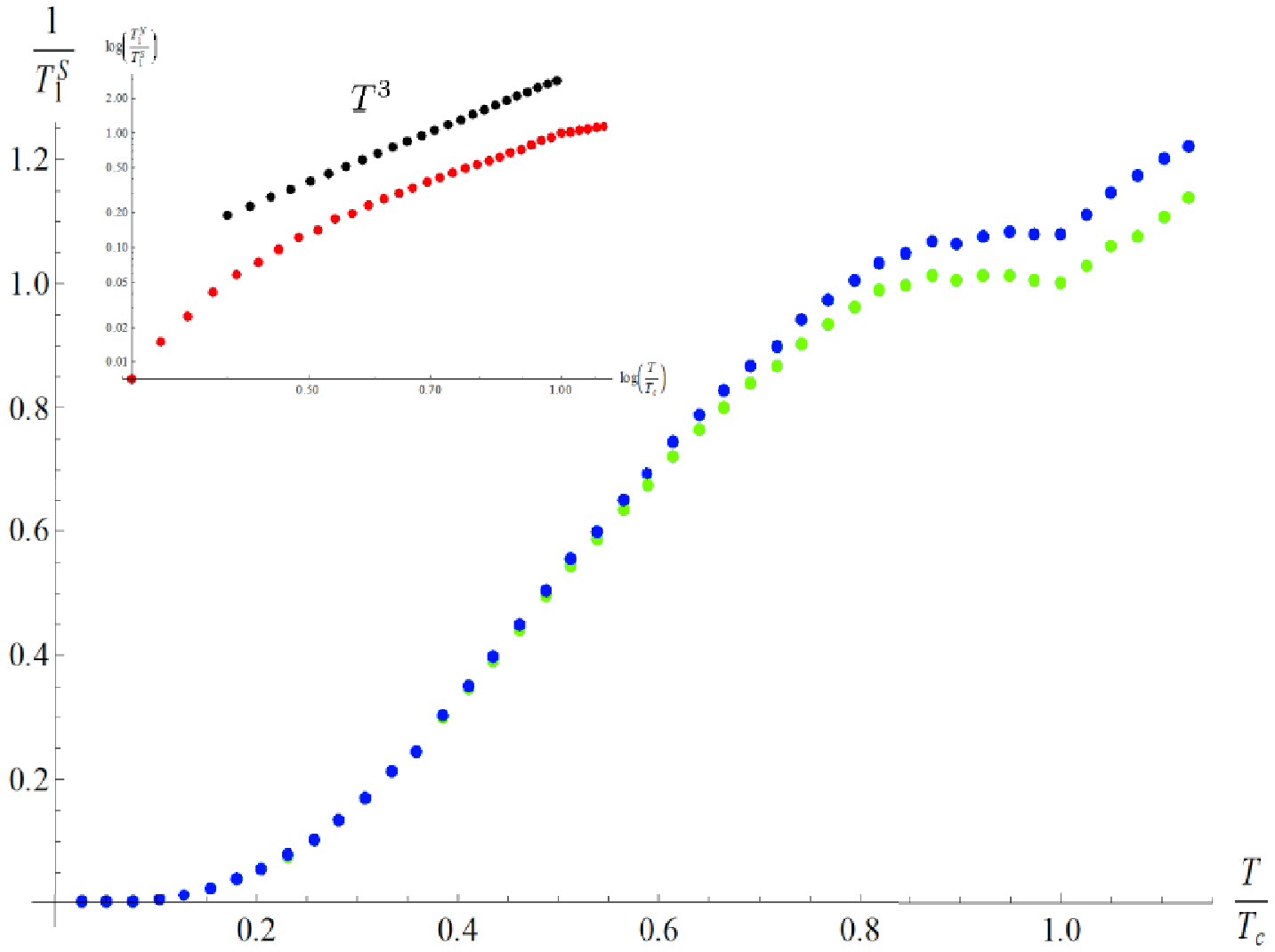
We predict that future experiments will see a small coherence peak resulting from the intra-band contribution. Our results show that, barring different scattering rates for inter- and intra-band scattering, the overall intra-band contribution to the NMR relaxation rate is roughly a factor of $5$ times larger than the inter-band contribution. This can also be argued on general grounds, provided that the hypothesis of weak-coupling theories and LDA (i.e. there is a quasi-nesting of the electron and hole Fermi surfaces in the parent material) is correct. Upon doping with either electrons or holes, either the electron or hole Fermi surfaces will become considerably larger than the other one. This means that the inter-band contribution to the NMR spin relaxation rate diminishes: it of course vanishes if one could, theoretically, deplete one of the Fermi pockets. Meanwhile, the intra-band contribution should, on general grounds, remain roughly constant upon doping because the overall size of the sum of the Fermi surfaces is relatively constant. All these general arguments are supported by our explicit calculation.

A few other remarks about the NMR spin relaxation rates are in order: (i) The observed $T^{3}$ temperature dependence of $1/T_{1}$ cannot be viewed as evidence against $s$-wave pairing symmetries. In fact, the temperature dependence just below $T_{c}$ is very sensitive to the ratio $\Delta/k_{B}T_{c}$. We find that the $T^{3}$ behavior can be obtained by choosing $\Delta/k_{B}T_{c}\sim 2$ for our large gap value, and the power of the temperature dependence can increase even further by increasing this ratio. (ii) Although we predict that there should be a coherence peak in the clean limit, impurities can efficiently reduce the coherence peak in a two-band system. A weak inter-band impurity scattering but strong intra-band scattering can suppress the coherence peak. This has been investigated in MgB₂[33] where the coherence peak is also not easily observed experimentally [34]. Since the superconductivity in Fe-based superconductors is created by doping, it is reasonable to assume that disorder is stronger than that in MgB₂. To observe the coherence peak, we require a very clean sample. (iii) Our calculation is based on a two-band model. This model can be over-simplified when one tries to use it to predict quantitative experimental measurements. For example, the detailed shape of Fermi surfaces and its doping dependence may not be quantitatively accurate. Therefore, the predictions in this paper with regard to doping concentration should be viewed as qualitative.

We have calculated the spectral function, the DOS, the tunneling differential conductance, the penetration depth, and the NMR spin relaxation rate for different superconducting order parameters in the iron-pnictides. We have emphasized that the nodal structure of the $s_{x^{2}y^{2}}$ order parameter will result in a qualitative change in these experimental observables with increasing doping, as the superconductor crosses over from gapped to gapless. Thus, one can in principle probe the existence of this pairing symmetry in the iron-pnictides by analyzing the behavior of the spectral function, the DOS and the penetration depth as a function of doping. For the $1/T_{1}$ NMR spin relaxation rate, if only the inter-band contribution is considered, our theoretical results are consistent with the current experimental results, including the $T^{3}$ behavior and the absence of a coherence peak. However, by including the intra-band contribution, a small coherence peak at the transition temperature will be present in a clean sample although it is smaller than that in a sign-unchanged $s$-wave.

Note – During the completion of this work, we became aware of two recent papers that also calculate the spin-lattice relaxation rate for the $s_{x^{2}y^{2}}$ order parameter in the iron-pnictides [35, 36], and another recent paper that considers the experimental consequences of two different pairing symmetries [37].

BAB wishes to thank P.W. Anderson, S. Sondhi, N.P. Ong, Z. Hasan, A. Yazdani, for discussions and comments. MMP and BAB are especially grateful to David Huse for fruitful discussions. JPH thanks Pengcheng Dai, S. Kivelson, X. Tao, E. W. Carlson, G. Q. Zheng, I.I. Mazin, H. Yao, for important discussion. JPH was supported by the National Science Foundation under grant No. PHY-0603759. MMP and BAB are supported by PCTS fellowships.

References

- [1] K. Seo, B. A. Bernevig, and J. Hu, eprint arXiv:0805.2958.
- [2] Y. Kamihara, T. Watanabe, M. Hirano, and H. Hosono, J. Am. Chem. Soc. 130, 3296 (2008).
- [3] H. Takahashi, K. Igawa, K. Arii, Y. Kamihara, M. Hirano, and H. Hosono, Nature 453, 376 (2008).
- [4] Z.-A. Re, J. Yang, W. Lu, W. Yi, G.-C. Che, X.-L. Dong, L.-L. Sun, and Z.-X. Zhao, eprint arXiv:0803.4283.
- [5] G. F. Chen, Z. Li, G. Li, J. Zhou, D. Wu, J. Dong, W. Z. Hu, P. Zheng, Z. J. Chen, J. L. Luo, et al., eprint arXiv:0803.0128.
- [6] X. H. Chen, T. Wu, G. Wu, R. H. Liu, H. Chen, and D. F. Fang, eprint arXiv:0803.3603.
- [7] H.-H. Wen, G. Mu, L. Fang, H. Yang, and X. Zhu, Europhys. Lett. 82, 17009 (2008).
- [8] M. Rotter, M. Tegel, and D. Johrendt, eprint arXiv:0805.4630.
- [9] K. Sasmal, B. Lv, B. Lorenz, A. Guloy, F. Chen, Y. Xue, and C. W. Chu, eprint arXiv:0806.1301.
- [10] G. F. Chen, Z. Li, G. Li, W. Z. Hu, J. Dong, X. D. Zhang, P. Zheng, N. L. Wang, and J. L. Luo, eprint arXiv:0806.1209.
- [11] V. Cvetkovic and Z. Tesanovic, eprint arXiv:0804.4678.
- [12] F. Ma, Z.-Y. Lu, and T. Xiang, eprint arXiv:0806.3526.
- [13] T. Yildirim, eprint arXiv:0804.2252.
- [14] Q. Si and E. Abrahams, eprint arXiv:0804.2480.
- [15] H. A. Mook, Y. Sidis, B. Fauqué, V. Balédent, and P. Bourges, eprint arXiv:0802.3620.
- [16] C. Fang, H. Yao, W.-F. Tsai, J. Hu, and S. A. Kivelson, Phys. Rev. B 77, 224509 (2008).
- [17] C. Xu, M. Mueller, and S. Sachdev, eprint arXiv:0804.4293.
- [18] I. I. Mazin, D. J. Singh, M. D. Johannes, and M. H. Du, eprint arXiv:0803.2740.
- [19] Y. Chen, J. W. Lynn, J. Li, G. Li, G. F. Chen, J. L. Luo, N. L. Wang, P. Dai, C. dela Cruz, and H. A. Mook, arXiv:0807.0662 (2008).
- [20] C. de la Cru, Q. Huang, J. W. Lynn, J. Li, W. R. II, J. L. Zarestky, H. A. Mook, G. F. Chen, J. L. Luo, N. L. Wang, et al., Nature 453, 899 (2008).
- [21] J. Zhao, Q. Huang, C. de la Cruz, S. Li, J. W. Lynn, Y. Chen, M. A. Green, G. F. Chen, G. Li, Z. Li, et al., arXiv:0806.2528 (2008a).
- [22] J. Zhao, W. R. II, J. W. Lynn, G. F. Chen, J. L. Luo, N. L. Wang, J. Hu, and P. Dai, arXiv:0807.1077 (2008b).
- [23] S. Raghu, X.-L. Qi, C.-X. Liu, D. Scalapino, and S.-C. Zhang, eprint arXiv:0804.1113.
- [24] L. Malone, J. D. Fletcher, A. Serafin, A. Carrington, N. D. Zhigadlo, Z. Bukowski, S. Katrych, and J. Karpinski, eprint arXiv:0806.3908.
- [25] K. Hashimoto, T. Shibauchi, T. Kato, K. Ikada, R. Okazaki, H. Shishido, M. Ishikado, H. Kito, A. Iyo, H. Eisaki, et al., eprint arXiv:0806.3149.
- [26] C. Martin, R. T. Gordon, M. A. Tanatar, M. D. Vannette, M. E. Tillman, E. D. Mun, P. C. Canfield, V. G. Kogan, G. D. Samolyuk, J. Schmalian, et al., eprint arXiv:0807.0876.
- [27] O. Fischer, M. Kugler, I. Maggio-Aprile, C. Berthod, and C. Renner, Rev. Mod. Phys. 79, 353 (2007).
- [28] K. Matano, Z. Ren, X. Dong, L. Sun, Z. Zhao, and G. qing Zheng, ArXiv:0806.0249 (2008).
- [29] H.-J. Grafe, D. Paar, G. Lang, N. J. Curro, G. Behr, J. Werner, J. Hamann-Borrero, C. Hess, N. Leps, R. Klingeler, et al., eprint arXiv:0805.2595.
- [30] Y. Nakai, K. Ishida, Y. Kamihara, M. Hirano, and H. Hosono, eprint arXiv:0804.4765.
- [31] H. Mukuda, N. Terasaki, H. Kinouchi, M. Yashima, Y. Kitaoka, S. Suzuki, S. Miyasaka, S. Tajima, K. Miyazawa, P. Shirage, et al., eprint arXiv:0806.3238.
- [32] N. Bulut and D. J. Scalapino, Phys. Rev. Lett. 68, 706 (1992).
- [33] B. Mitrovic and K. V. Samokhin, Phys. Rev. B 74, 144510 (2006).
- [34] H. Kotegawa, K. Ishida, Y. Kitaoka, T. Muranaka, and J. Akimitsu, Phys. Rev. Lett 87, 127001 (2001).
- [35] D. Parker, O. V. Dolgov, M. M. Korshunov, A. A. Golubov, and I. I. Mazin, eprint arXiv:0807.3729.
- [36] A. V. Chubukov, D. Efremov, and I. Eremin, eprint arXiv:0807.3735.
- [37] Y. Bang and H.-Y. Choi, eprint arXiv:0807.3912.