Elastic Theory of Defects in Toroidal Crystals

The study of the spontaneous organization of microscopic objects such as colloids, amphiphiles or protein clusters into mesoscale structures (mesoatoms) is an active research area that offers challenges on many fronts [1, 2]. One would like to create a rich warehouse of raw materials from which to engineer mesomolecules or bulk materials with novel mechanical, optical or electronic behavior.

A fertile source of potential mesoatoms is provided by the self-assembly of micron or smaller scale colloidal particles on curved interfaces. The interplay between spatial curvature and condensed matter order in these systems has proven to be very rich. Spatial curvature leads to novel defect arrays in the ground state that have widespread implications for the fundamental and applied physics of curved phases of matter with crystalline, hexatic or nematic order.

In a recent paper Kim et al reported the formation of toroidal micelles from the self-assembly of dumbbell-shaped amphiphilic molecules [3]. Molecular dumbbells dissolved in a selective solvent self-assemble in an aggregate structure due to their amphiphilic character. This process has been observed to yield coexisting spherical and open-ended cylindrical micelles. These structures change slowly over the course of a week to toroidal micelles which thus appear more stable. Toroidal geometries also occur in microbiology in the viral capsid of the coronavirus torovirus [4]. The torovirus is an RNA viral package of maximal diameter between $120$ and $140$ nm and is surrounded, as other coronaviridae, by a double wreath/ring of cladding proteins.

Carbon nanotori form another fascinating and technologically promising class of toroidal crystals [5] with remarkable magnetic and electronic properties. The interplay between the ballistic motion of the $\pi$ electrons and the geometry of the embedding torus leads to a rich variety of quantum mechanical properties including Pauli paramagnetism [6] and Aharonov-Bohm oscillations in the magnetization [7]. Ring closure of carbon nanotubes by chemical methods [8] suggest that nanotubes may be more flexible than at first thought and provides another technique of constructing carbon tori.

A unified theoretical framework to describe the structure of toroidal crystals is provided by the elastic theory of defects in a curved background [9, 10, 11, 12]. This formalism has the advantage of far fewer degrees of freedom than a direct treatment of the microscopic interactions and allows one to explore the origin of the emergent symmetry observed in toroidal crystals as the result of the interplay between defects and geometry. The latter is one of the fundamental hallmarks of two-dimensional non-Euclidean crystals and leads to universal features observed in systems as different as viral capsids and carbon macromolecules.

In this paper we provide a detailed analysis of the structural properties of toroidal crystals. We show that the ground state has excess $5-$fold disclination defects on the exterior of the torus and $7-$fold defects on the interior. The precise number of excess disclinations, as well as their arrangement, is primarily controlled by the aspect ratio of the torus. Since defective regions are physically distinguished locations they are natural places for biological activity and chemical functionalization. A thorough understanding of the surface structure of crystalline assemblages could represent a significant step towards a first-principles design of entire libraries of nano and mesoscale components with precisely determined valence. Such mesoatoms could serve in turn as the building blocks for mesomolecules or bulk materials via spontaneous self-assembly or controlled fabrication.

The paper is organized as follows. In Sec. II we review the elastic theory of defects in two-dimensional curved geometries and derive the ground state energy of a toroidal crystal. In Sec. III we summarize some fundamentals of the geometry of triangulated tori and discuss how the intrinsically discrete problem of crystallography can be reconciled with the result of the continuous elastic theory presented in the previous section. Sec. IV is devoted to the analysis of the crystalline structure arising from the solution of the elastic problem. In Sec. V we discuss the results of numerical minimization of the potential energy of a system of classical particles interacting via a short-range potential on the surface of a torus in the light of the results of Sec. IV. Finally, in Sec. VI we specialize our analysis to the case of a “fat torus” of aspect ratio one and we show how the curvature singularity at the center of the torus is responsible for a remarkable curvature-driven transition to a disordered state. Some of the results presented here have been already announced in Ref. 13.

A two-dimensional torus of revolution $T^{2}$ is described in parametric form by:

$$\left\{\begin{array}[]{l}x=(R_{1}+R_{2}\cos\psi)\cos\phi\\ y=(R_{1}+R_{2}\cos\psi)\sin\phi\\ z=R_{2}\sin\psi\end{array}\right.\,,$$

(1)

where $R_{1}>R_{2}$ are the two radii of the torus. The metric tensor $g_{ij}$ (with determinant $g$) and the Gaussian curvature $K$ can be written respectively as:

	$$\displaystyle g_{ij}=\left(\begin{array}[]{cc}R_{2}^{2}&0\\ 0&(R_{1}+R_{2}\cos\psi)^{2}\end{array}\right)\,,$$
	$$\displaystyle K=\frac{\cos\psi}{R_{2}(R_{1}+R_{2}\cos\psi)}\,.$$		(4)

Within the elastic theory of defects on curved surfaces the original interacting particle problem is mapped to a system of interacting disclination defects in a continuum elastic curved background. Disclinations are characterized by their topological or disclination charge, $q_{i}$, representing the departure of a vertex from a the $6-$fold coordination of a perfect triangular lattice. Thus $q_{i}=6-c_{i}$, where $c_{i}$ is the coordination number of the $i$th vertex. A classic theorem of Euler requires the total disclination charge of any triangulation of a two-dimensional Riemannian manifold $M$ to equal $6\chi_{M}$, where $\chi_{M}$ is the Euler characteristic of $M$. In the case of the torus $\chi_{M}=0$, and thus disclinations must appear in pairs of opposite disclination charge (i.e. $5-$fold and $7-$fold vertices with $q_{i}=1$ and $-1$ respectively) in order to ensure disclination charge neutrality.

The total free energy of a toroidal crystal with $N$ disclinations can be expressed as

$$F=\frac{1}{2Y}\int d^{2}x\,\Gamma^{2}(\bm{x})+\epsilon_{c}\sum_{i=1}^{N}q_{i}^{2}+F_{0}\,,$$

(5)

where $Y$ is the 2D Young modulus and $\Gamma(\bm{x})$ is the solution of the following Poisson problem with periodic boundary conditions:

$$\Delta_{g}\Gamma(\bm{x})=Y\rho(\bm{x})\,,$$

(6)

where $\Delta_{g}$ is the Laplace-Beltrami operator

$$\Delta_{g}=g^{ij}\nabla_{i}\nabla_{j}=\frac{1}{\sqrt{g}}\,\partial_{i}\sqrt{g}\,g^{ij}\partial_{j}$$

(7)

and $\rho(\bm{x})$ is the total topological charge density

$$\rho(\bm{x})=\frac{\pi}{3}\sum_{k=1}^{N}q_{k}\delta(\bm{x},\bm{x}_{k})-K(\bm{x})$$

(8)

of $N$ disclinations located at the sites $\bm{x}_{k}$ together with the screening contribution due to the Gaussian curvature $K(\bm{x})$ of the embedding manifold.

The first term in Eq. (5) represents the long-range elastic distortion due to defects and curvature. The second term in Eq. (5) is the defect core-energy representing the energy required to create a single disclination defect. This quantity is related to the short-distance cut-off of the elastic theory and is proportional to the square of the topological charge times a constant $\epsilon_{c}$ [14]. Finally $F_{0}$ is the free energy of a flat defect-free monolayer. The Gauss-Bonnet theorem [15] requires the total topological charge to be zero on the torus:

$$\sum_{k=1}^{N}q_{k}=\int d^{2}x\,K(\bm{x})=0$$

(9)

The function $\Gamma(\bm{x})$ can be expressed in the Green form:

$$\frac{\Gamma(\bm{x})}{Y}=\int d^{2}y\,G_{L}(\bm{x},\bm{y})\rho(\bm{y})\,,$$

(10)

where $G_{L}(\bm{x},\bm{y})$, the Laplacian Green function on the torus, satisfies the equation:

$$\Delta_{g}G_{L}(\bm{x},\bm{y})=\delta_{g}(\bm{x},\bm{y})-A^{-1}\,,$$

(11)

with $\delta_{g}(\bm{x},\bm{y})$ the Dirac delta function on the torus and $A=4\pi^{2}R_{1}R_{2}$ is the surface area. It is easy to prove that the solution of the traditional Green-Laplace equation doesn’t exist on closed manifolds like the torus, from which the extra term $A^{-1}$ appearing in Eq. (11). $A^{-1}$ is the eigenfunction of the Laplacian associated with the null eigenvalue (zero mode) and is necessary because a pure isolated source (giving rise to the delta-function on the right-hand side) has no place to terminate the field on the closed torus.

As usual the calculation of the Green function can be remarkably simplified by conformally mapping the torus to a domain of the Euclidean plane via a suitable system of isothermal coordinates. Intuitively the torus is conformally equivalent to a rectangular domain described by a system of Cartesian coordinates. To make this explicit, one can equate the metric of the torus in the coordinates $(\psi,\phi)$ to a conformally Euclidean metric in the coordinates $(\xi,\eta)$:

$$ds^{2}=R_{2}^{2}d\psi^{2}+(R_{1}+R_{2}\cos\psi)^{2}d\phi^{2}=w\,(d\xi^{2}+d\eta^{2})\,,$$

where $w$ is a positive conformal factor. Taking $\eta=\phi$ and $w=(R_{1}+R_{2}\cos\psi)^{2}$, the coordinate $\xi$ is determined by the differential equation:

$$\frac{d\xi}{d\psi}=\pm\frac{1}{r+\cos\psi}\,,$$

(12)

where $r=R_{1}/R_{2}$, the aspect ratio of the torus, may be taken greater or equal to one without loss of generality. Choosing the plus sign and integrating both sides of Eq. (12) we find:

$$\xi=\int_{0}^{\psi}\frac{d\psi^{\prime}}{r+\cos\psi^{\prime}}\,.$$

(13)

Taking $\psi\in[-\pi,\pi]$, the integral (13) yields:

$$\xi=\kappa\atan\left(\omega\tan\frac{\psi}{2}\right)\,,$$

where

$$\kappa=\frac{2}{\sqrt{r^{2}-1}}\,,\qquad\qquad\omega=\sqrt{\frac{r-1}{r+1}}\,.$$

(14)

In the transformed coordinate system $(\xi,\eta)$ the modified Green-Laplace equation reads:

$$\Delta G_{L}(\bm{x},\bm{y})=\delta(\bm{x},\bm{y})-\frac{w}{A}\,,$$

(15)

where $\Delta$ and $\delta$ are now the Euclidean Laplacian and delta function. The function $G_{L}(\bm{x},\bm{y})$ can be expressed in the form:

$$G_{L}(\bm{x},\bm{y})=G_{0}(\bm{x},\bm{y})-\langle G_{0}(\bm{x},\cdot\,)\rangle-\langle G_{0}(\cdot\,,\bm{y})\rangle+\langle G_{0}(\cdot\,,\cdot\,)\rangle\,,$$

where $G_{0}(\bm{x},\bm{y})$ is the Laplacian Green function on a periodic rectangle and the angular brackets stand for the normalized integral of the function $G_{0}(\bm{x},\bm{y})$ with respect to the dotted variable:

$$\langle G_{0}(\bm{x},\cdot\,)\rangle=\int\frac{d^{2}y}{A}\,G_{0}(\bm{x},\bm{y})\,.$$

(16)

Analogously the function $\langle G_{0}(\cdot\,,\cdot\,)\rangle$ is given by

$$\langle G_{0}(\cdot\,,\cdot\,)\rangle=\int\frac{d^{2}x\,d^{2}y}{A^{2}}\,G_{0}(\bm{x},\bm{y})$$

and ensures the neutrality property:

$$\int d^{2}x\,G_{L}(\bm{x},\bm{y})=\int d^{2}y\,G_{L}(\bm{x},\bm{y})=0\,.$$

(17)

Using standard analysis the Green function $G_{0}(\bm{x},\bm{y})$ at the points $\bm{x}=(\xi,\eta)$ and $\bm{y}=(\xi^{\prime},\eta^{\prime})$ of a periodic rectangle of edges $p_{1}$ and $p_{2}$ can be calculated in the form:

$$G_{0}(\bm{x},\bm{y})=\frac{\log 2}{6\pi}-\frac{1}{2\,p_{1}p_{2}}|\eta-\eta^{\prime}|^{2}\\[7.0pt] +\frac{1}{2\pi}\log\left|\frac{\vartheta_{1}(\frac{z-z^{\prime}}{p_{1}/\pi}|\frac{ip_{2}}{p_{1}})}{\vartheta_{1}^{\prime\frac{1}{3}}(0|\frac{ip_{2}}{p_{1}})}\right|\,,$$

(18)

where $z=\xi+i\eta$, $z^{\prime}=\xi^{\prime}+i\eta^{\prime}$ and $\vartheta_{1}$ is the Jacobian theta function and reflects the double periodicity of the torus [30]. A pedagogical derivation of the Green function $G_{0}(\bm{x},\bm{y})$ is reported in Appendix A. Substituting Eq. (18) in Eq. (10) with $p_{2}=2\pi$ and

$$p_{1}=2\int_{0}^{\pi}\frac{d\psi}{r+\cos\psi}=\kappa\pi\,,$$

we obtain:

$$\Gamma(\bm{x})=\frac{\pi}{3}\sum_{k=1}^{N}q_{k}\Gamma_{d}(\bm{x},\bm{x}_{k})-\Gamma_{s}(\bm{x})\,,$$

(19)

where $\Gamma_{s}(\bm{x})$ represents the stress field due to the Gaussian curvature of the torus and is given by:

$$\frac{\Gamma_{s}(\bm{x})}{Y}=\log\left[\frac{r+\sqrt{r^{2}-1}}{2(r+\cos\psi)}\right]+\frac{r-\sqrt{r^{2}-1}}{r}\,.$$

(20)

The function $\Gamma_{d}(\bm{x},\bm{x}_{k})$ is the stress field at the point $\bm{x}$ arising from the elastic distortion due to a defect at $\bm{x}_{k}$ and is given by

	$$\displaystyle\frac{\Gamma_{d}(\bm{x},\bm{x}_{k})}{Y}=\frac{\kappa}{16\pi^{2}}\left(\psi_{k}-\frac{2}{\kappa}\,\xi_{k}\right)^{2}-\frac{1}{4\pi^{2}\kappa}(\phi-\phi_{k})^{2}$$
	$$\displaystyle+\frac{1}{4\pi^{2}r}\log(r+\cos\psi_{k})-\frac{\kappa}{4\pi^{2}}\Real\{\Li(\alpha e^{i\psi_{k}})\}$$
	$$\displaystyle+\frac{1}{2\pi}\log\left|\vartheta_{1}\left(\frac{z-z_{k}}{\kappa}\bigg|\frac{2i}{\kappa}\right)\right|\,,$$		(21)

where $\Li$ is the usual Eulerian dilogarithm and

$$\alpha=\sqrt{r^{2}-1}-r\,.$$

(22)

A derivation of the functions $\Gamma_{s}(\bm{x})$ and $\Gamma_{d}(\bm{x},\bm{x}_{k})$ is given in Appendix B. Integrating the function $\Gamma(\bm{x})$ on the torus gives the elastic energy of an arbitrary collection of disclinations. A detailed analysis of the crystalline structure arising from Eqs. (5), (19), (20) and (21) is carried out in Sec. III.

Before analyzing the defect distribution arising from the elastic energy of Eq. (5), together with Eq. (19), it is necessary to understand the geometry of triangulated tori. Reconciling the predictions of a continuum elastic theory with the intrinsically discrete nature of crystallography requires an understanding of the possible lattices that can be embedded on the torus and the associated defects. The problem of classifying the possible triangulations of the $2-$torus has received considerable attention from mathematicians, physicists and chemists over the past twenty years. Lavrenchenko [16] proved in 1984 that all the triangulations of the torus can be generated from 21 irreducible triangulations by certain sequences of operations called vertex splitting ¹¹ 1 Analogously it can be proved that the number of irreducible triangulations is one for the sphere and two for the projective plane. The extraordinary larger value obtained for the torus should be indicative of the high structural complexity of a crystalline torus.. After the discovery of carbon nanotubes in 1991 and the subsequent theoretical construction (later followed by the experimental observation) of graphitic tori, many possible tessellations of the circular torus have been proposed by the community [17, 18, 19, 20, 21]. In this section we review the construction of a defect-free triangulated torus and we show how the most symmetric defective triangulations can be generally grouped into two fundamental classes corresponding to symmetry groups $D_{nh}$ and $D_{nd}$ respectively.

For the sake of consistency with the existing literature we adopt here the language developed to describe the structure of carbon nanotubes. The structure of a triangulated cylinder can be specified by a pair of triangular lattice vectors $\bm{c}$ and $\bm{t}$, called the chiral and translation vector respectively, which together define how the planar lattice is rolled up. In the canonical basis $\bm{a_{1}}=(1,0)$ and $\bm{a}_{2}=(\frac{1}{2},\frac{\sqrt{3}}{2})$, the vector $\bm{c}$ has the form:

$$\bm{c}=n\bm{a}_{1}+m\bm{a}_{2}\qquad n,\,m\in\mathbb{Z}\,.$$

(23)

The translation vector $\bm{t}$, on the other hand, can be expressed as an integer multiple

$$\bm{t}=l\bm{e}_{t}\qquad l\in\mathbb{Z}$$

(24)

of the shortest lattice vector $\bm{e}_{t}$ perpendicular to $\bm{c}$. The vector $\bm{e}_{t}$ is readily found to be of the form:

$$\bm{e}_{t}=\frac{(n+2m)\bm{a}_{1}-(2n+m)\bm{a}_{2}}{(n+2m:2n+m)}\,,$$

where $(a:b)$ denotes the greatest common divisor of $a$ and $b$ and enforces the minimal length. The three-dimensional structure of the torus is obtained by connecting the edge $\overline{OT}$ of the rectangle in Fig. 2 (top) to $\overline{O^{\prime}C}$ and $\overline{OC}$ to $\overline{O^{\prime}T}$. The edge $\overline{OT}$ is then mapped to the external equator of the torus while the edge $\overline{OC}$ to the $\phi=0$ meridian. The resultant toroidal lattice has characteristic chirality related to the initial choice of the vector $\bm{c}$. In the nanotubes literature armchair referes to the lattice obtained by choosing $n=m$, zigzag to that obtained for $m=0$ and chiral to all other lattices. An example of a $(n,m,l)$ chiral torus is shown in Fig. 2 (bottom) for the case $n=6$, $m=3$ and $l=6$. The chirality is extremely important in graphitic carbon nanotube or nanotori, where it determines whether the electronic behavior of the system is metallic or semiconducting.

By Euler’s theorem one can prove that the number of triangular faces $F$ and the number of vertices $V$ of a triangular toroidal lattice is given by:

$$V=\tfrac{1}{2}F\,.$$

Denoting $A_{R}$ the area of the rectangle with edges $\bm{c}$ and $\bm{t}$ and $A_{T}$ the area of a fundamental equilateral triangle, the number of vertices of a defect-free toroidal triangulation is then:

$$V=\frac{A_{R}}{2A_{T}}=\frac{2l\,(n^{2}+nm+m^{2})}{(n+2m:2n+m)}\,.$$

(25)

The planar construction reviewed above allows only lattices with an even number of vertices. Defect-free toroidal deltahedra with an odd number of vertices are also possible and their construction is generally achieved by assembling congruent octahedral building blocks. An example of this scheme will be briefly discussed in Sec. V for the case $V=87$ and $r=6$. We refer the reader to Ref. 22 for an comprehensive review of the topic.

The embedding of an equal number of pentagonal and heptagonal disclinations in the hexagonal network was first proposed by Dunlap in 1992 as a possible way to incorporate positive and negative Gaussian curvature into the cylindrical geometry of carbon tubules [17]. According to the Dunlap construction the necessary curvature is incorporated by the insertion of “knees” (straight cylindrical sections of the same diameter joined with a kink) in correspondence with each pentagon-heptagon pair arising from the junction of tubular segments of different chirality (see Fig. 4).

In particular, a junction between a $(n,0)$ and a $(m,m)$ tube can be obtained by placing a $7-$fold disclination along the internal equator of the torus and a $5-$fold disclination along the external equator. Since the radii of the two segments of a junction are different by construction, the values of $n$ and $m$ are commonly chosen to minimize the ratio $|\bm{c}_{(n,0)}|/|\bm{c}_{(m,m)}|=n/\sqrt{3}m$. By repeating the $5-7$ construction periodically it is possible to construct an infinite number of toroidal lattices with an even number of disclinations pairs and dihedral symmetry group $D_{nh}$ (where $2n$ is the total number of $5-7$ pairs, Fig 5). The structure of the lattice is described by the alternation of two motifs with crystalline axes mutually rotated by $30^{\circ}$ as a consequence of the connecting disclination. One of the fundamental aspects of Dunlap’s construction is that all the disclinations are aligned along the two equators of the torus where the like-sign Gaussian curvature is maximal. As we will see below, this feature makes these arrangements optimal in releasing the elastic stress due to curvature.

Another class of crystalline tori with dihedral antiprismatic symmetry $D_{nd}$ was initially proposed by Itoh et al [18] shortly after Dunlap. Aimed at reproducing a structure similar to the C₆₀ fullerene, Itoh’s original construction implied ten disclination pairs and the point group $D_{5d}$. In contrast to Dunlap tori, disclinations are never aligned along the equators in antiprismatic tori, instead being staggered at some angular distance $\delta\psi$ from the equatorial plane. Hereafter we will use the symbol TA$n$ to refer to toroidal deltahedra with $2n$ disclination pairs and $D_{nd}$ symmetry group.

A systematic construction of defected triangulations of the torus can be achieved in the context of planar graphs [16, 29]. A topological embedding of a graph in a two-dimensional manifold corresponds to a triangulation of the manifold if each region of the graph is bounded by exactly three vertices and three edges, and any two regions have either one common vertex or one common edge or no common elements of the graph. The simplest example of toroidal polyhedra with $D_{nd}$ symmetry group, featuring only $5-$fold and $7-$fold vertices, can be constructed by repeating $n$ times the unit cell of Fig. 7a. These toroidal antiprisms ²² 2 Although we presume this class of toroidal polyhedra is not discussed here for the first time, we couldn’t find any previous reference in the literature. have $V=4n$ vertices and can be obtained equivalently from the edge skeleton of a $n-$fold antiprism by attaching at each of the base edges a pentagonal pyramid and by closing the upper part of the polyhedron with $n$ additional triangles. By counting the faces one finds $F=5n+2n+n=8n$ from which $V=4n$. The simplest polyhedron of this family has $V=12$ and $D_{3d}$ symmetry group (see top left of Fig. 6) and corresponds to the “drilled icosahedron” obtained by removing two parallel faces of an icosahedron and connecting the corresponding edges with the six lateral faces of an antiprism with triangular base (i.e. a prolate octahedron). Starting from this family of toroidal antiprisms a number of associated triangulations having the same defect structure can be obtained by geometrical transformations such as the Goldberg inclusion [23, 24, 25]. Such transformations, popularized by Caspar and Klug for the construction of the icosadeltahedral structure of spherical viruses [24], consist in partitioning each triangular face of the original graph into smaller triangular faces in such a way that old vertices preserve their valence and new vertices have valence six. The partition is obtained by specifying two integer numbers $(L,M)$ which define how the original vertices of each triangle are connected by the new edges so that the total number of vertices is increased by a factor $T=L^{2}+LM+M^{2}$.

A general classification scheme for $D_{nd}$ symmetric tori was provided by Berger and Avron [29] in 1995. Their scheme is based on the construction of unit graphs comprising triangular tiles of different generations. In each generation, tiles are scaled in length by a factor $1/\sqrt{2}$ with respect to the previous generation. This rescaling approximates the non-uniformity of the metric of a circular torus.

Dunlap toroids can be obtained from unit cells such as those shown in Fig. 8. The geometrical properties of these graphs can be described in different ways. A particularly intuitive way, in the spirit of this paper, consists in specifying the distances between $5-$ and $7-$fold pairs. One starts by drawing the smallest convex loop passing through defective sites. This identifies a central polygon whose upper vertices ($v_{1}$ and $v_{2}$ in Fig.9) have degree five and lower vertices ($v_{5}$ and $v_{6}$ in Fig. 9) have degree seven. Then calling $a$ the distance between $5-$fold vertices $v_{1}$ and $v_{2}$, $b$ that between $7-$fold vertices $v_{5}$ and $v_{6}$ and $c$ the length of the segment $\overline{v_{3}v_{4}}$ ($d=a$ for a trapezoid), we can express the total number of triangles enclosed by the central polygon as:

$$f=2c^{2}-a^{2}-b^{2}\,.$$

Each $7-$fold vertex sits at the apex of a diamond-shaped complex of $f^{\prime}=7$ triangles. Each $5-$fold vertex, on the other hand, is at the apex of a triangular region of $f^{\prime\prime}=(c-a+1)^{2}$ triangles. The graph is completed by a rectangle of height $c-a+4$ and base of arbitrary length $2d$ containing:

$$f^{\prime\prime\prime}=4d(c-a+4)$$

triangles. The total number of vertices is

	$\displaystyle V_{g}$	$\displaystyle=f+f^{\prime}+f^{\prime\prime}+f^{\prime\prime\prime}/2$
		$\displaystyle=c^{2}-b^{2}+2(c-a)(c+d+1)+8(d+1)\,.$		(26)

The final triangulation of the torus is obtained by repeating the prismatic unit cell $l$ times and therefore has $V=lV_{g}$ vertices. This scheme provides direct information on the arrangement of defective sites. Thus for instance an $(a,b,c,d)=(2,1,3,1)$ unit cell (see top of Fig. 8) has $5-$fold vertices separated by two lattice spacings and $7-$fold vertices by one lattice spacing. On the other hand the integers $n$ and $m$ giving the chirality of the two segments of the junction $(n,0)/(m,m)$ are given directly by as:

	$\displaystyle n$	$\displaystyle=c-a+4$
	$\displaystyle m$	$\displaystyle=2c-a-b\,.$

Thus the $(2,1,3,1)$ cell of Fig. 8 is obtained from the junction between a $(5,0)$ and a $(3,3)$ tubular segment.

Dunlap’s toroids are not the only examples of defective triangulations of the torus with dihedral prismatic symmetry group $D_{nh}$. With the help of numerical simulations (see Sec. V) we found two other classes whose unit cell is shown in Fig. 10. Unlike Dunlap’s toroids, the $7-$fold vertices in these prismatic triangulations are not aligned along the internal equator of the torus, but rather grouped in dimers normal to the equatorial plane. $5-$fold vertices are distributed along the external equator in the graph of Fig. 10a or form a double ring above and below it in the case of the graph Fig. 10b. Toroidal deltahedra obtained by embedding the prismatic graphs of Fig. 10 on a circular torus are shown in Fig. 11 for the case of a $5-$fold symmetric toroid with $V=35$ and a $7-$fold symmetric toroid with $V=49$. In the rest of the paper we will reserve the symbol TP$n$ for Dunalp’s toroids and refer with TP$n$a and TP$n$b to the other two classes of toroids with symmetry group $D_{nh}$ and unit cell of as shown in Fig. 10a and Fig. 10b respectively.

All defective triangulations presented so far are characterized by an even number of disclination pairs. Regular tessellations of the torus comprising an odd number of defects pairs are also possible. Such tessellations are obtained by combining segments of prismatic and antiprismatic lattices with a consequent loss of dihedral symmetry. Fig. 12 shows the Voronoi diagram of a toroidal lattice, with $r=10/3$ and $V=200$ vertices, containing 11 disclination pairs. For an angular length of approximately $\Delta\phi=7/5\,\pi$ the lattice is a prismatic $D_{5d}$ toroid while in the remaining $3/5\,\pi$ the local structure is that of an antiprismatic toroid. The global structure has only bilateral symmetry about a sagittal plane dividing the lattice in two mirror halves and thus point group $C_{s}$.

In the past few years, alternative constructions of triangulated tori have been proposed as well as novel geometrical and graph-theoretical methods to express the coordinates of their three-dimensional structures (see for example Kirby [19], László at al [20], Diudea et al [21]). Here we choose to focus on the defect structure associated with the two most important class TP$n$ and TA$n$ with groups $D_{nh}$ and $D_{nd}$.

In this section we report the result of a numerical minimization of a system of $V$ point-like particles constrained to lie on the surface of a torus and interacting via a pair potential of the form $U_{ij}=1/|\bm{x}_{i}-\bm{x}_{j}|^{3}$ where $|\cdot|$ denotes the Euclidean distance in $\mathbb{R}^{3}$. The problem of finding the minimal energy configuration of repulsively interacting points on a 2-manifold has become a standard problem of potential theory and has its paradigm in the classical Thomson problem on the sphere. The choice of the cubic potential is motivated here by the so called “poppy seed bagel theorem” [40], according to which the configuration of points that minimizes the Riesz energy $E=\sum_{i<j}1/|\bm{x}_{i}-\bm{x}_{j}|^{s}$ on a rectifiable manifold of Hausdorff dimension $d$ is uniformly distributed on the manifold for $s\geq d$. In the case of a torus of revolution this implies that for small $s$ the points are mostly distributed on the exterior of the torus (the interior becomes completely empty in the limit $V\rightarrow\infty$). As $s$ is increased, however, the points cover a progressively larger portion of the surface. The distribution becomes uniform for $s\geq 2$. On the other hand, since the number of local minima of the Riesz energy increases with $s$, it is practical to choose a value not much larger than two. The choice $s=3$ has the further advantage of modelling a real physical system of neutral colloidal particles assembled at an interface [41] and is therefore suitable for direct comparison with experiments on colloidal suspensions.

To construct low energy configurations we adopt an carefully designed hybrid optimization algorithm named Tapping (TA). Like other hybrid algorithms, TA consists in a combination of fast local optimizations and global stochastic moves designed to release the system from the local minimum to which it is confined at the end of a local minimization step. A more detailed description of our algorithm is reported in Appendix C. We study four different aspect ratios: $r=3\,,4\,,6$ and $20$. For each aspect ratio we consider several different particle numbers up to $V=1000$ and each simulation is performed for $10^{5}$ to $10^{6}$ TA iterations.

The lowest energies found, as well as the number of defects in the corresponding configuration, are reported in Table 2 for a selected set of systems. The corresponding lattices are shown in Fig. 20

The lattices are best presented using a Voronoi construction corresponding to the dual lattice of the Delaunay triangulation. Here pentagonal faces are colored in red while heptagonal faces are colored in blue. The complete set of data produced in our simulations together with a collection of interactive 3D graphics for each low energy configuration found is available on-line [42]. For fewer than $V\sim 180$ particles the results of our numerical minimization are in good agreement with the continuum elastic theory. In particular for $180<V<500$ and $r=3,\,4$ and $6$, we always find minimal energy configurations consisting of ten $5-$fold disclinations on the outside of the torus and ten $7-$fold disclinations in the inside as predicted by the elastic theory in the regime of $\epsilon_{c}/(AY)\sim 0$. For $r=20$ and $V>110$ we also find the lowest energy configurations to be defect free.

For small numbers of particles we don’t expect the continuum approximation to accurately describe the lowest energy structure of the toroidal clusters presented in Fig. 20. Loosely speaking the limit of validity of the elastic theory can be quantified by requiring the average lattice spacing $a=2\pi[R_{1}R_{2}/(\frac{\sqrt{3}}{2}V)]^{1/2}$ to be much smaller than the radius $R_{2}$ of the torus. This condition requires $V$ to be of order $500$ particles for a torus with aspect ratio $r=3$. Remarkably, good agreement between the theory and simulations is found starting from much smaller values of $V$ and in some cases (see the following discussion on the configuration with $r=3$ and $V=130$), we already observe the onset of the ideal behavior predicted by theory for $a\sim R_{2}$. The occurrence of a ground state configuration with exact prismatic or antiprismatic symmetry, in particular, is only possible when the number of particles $V$ belongs to a specific sequence of “magic numbers” described in Sec. III. Nevertheless for $V$ outside such a sequence it is still possible to observe in the ground state a predominant prismatic or antiprismatic character depending on the aspect ratio.

Some configurations deserve special attention. For $V=16,\,20,\,24,\,28$ and $32$ and $r$ within a specific range (see Table 1) the global minima are represented by the second to sixth toroidal antiprims discussed in Sec. III. The drilled icosahedron, on the other hand, would require the aspect ratio be less than one, as can be understood from Table 1, and is therefore never a minimum for $V=12$. We next describe the salient features of the four aspect ratios simulated.

$r=3$) The smallest minimal energy state with $D_{5h}$ symmetry is obtained for $V=35$. It features ten disclination pairs and belongs to the class of TP$5$a graphs. For $V=42$, a TP$6$b lattice is obtained with no defects along the two equators. Two $6-$fold chiral configurations are obtained for $V=60$ and $126$. The global minimum obtained for $V=130$ displays a fascinating example of $5-$fold antiprismatic symmetry with the ten isolated negative disclinations in the interior of the torus replaced by a simplicial complex consisting of five triangles with a common $5-$fold apex and four $7-$fold coordinated vertices along the base. A peculiar example is also represented by the minimum obtained for $V=180$. The lattice exhibits the typical pattern of a TP$n$ graph with $(3,1,4,7)-$type unit cell. The angular distance between neighboring disclinations is $\delta\phi\sim 2\pi/9$. Since a prismatic graph cannot have an odd number of disclination pairs the toroidal lattice is closed by a simplicial complex consisting of two positive disclinations on the exterior of the torus at the opposite sides of the external equator and two negative disclinations in the interior arranged similarly. The total number of disclination pairs is therefore ten. The typical pattern of the $5-$fold antiprismatic toroid can be found in all configurations with $V>200$. A single $5-7-5$ scar appears in the $r=3$ configurations at $V=420$, while larger lattices (i.e $V=460$ and $500$) also feature $4-$fold disclinations in the interior of the torus. It is not clear, however, whether the presence of disclinations with topological charge $|q|>1$ is a genuine property of the ground state or rather an artifact due to a misconvergence of our algorithm.

$r=4$) An interesting feature is observed at $V=42$. As in the case of $r=3$ we also find a minimum with $D_{6h}$ symmetry group, but unlike the latter configuration, it belongs to the TP$6$a class and has $5-$fold disclinations along the external equator. A TP$7$b configuration is obtained again for $V=49$. For $V=66$ and $V=104$ the global minimum is achieved by two spectacular antiprismatic configurations with $D_{11d}$ and $D_{13d}$ symmetry group respectively. These toroids can be obtained from the toroidal antiprisms discussed in Sec. III by splitting ³³ 3 Vertex splitting is a standard operation to generate larger triangulations from an irreducible one. It consists in dividing an existing vertex $v$ in two such that the total number of vertices is increased by one. The two newly created vertices have coordination number $c-1$, with $c$ is the coordination number $v$, while two of the $c$ neighbors of $v$ gain a bond. one or more times the initial set of $5-$fold vertices. Thus starting from a $11-$fold toroidal antiprism with $V=4\times 11=44$ vertices and splitting all $22$ $5-$fold vertices one obtains $V=44+22=66$ vertices. Splitting twice all $26$ $5-$fold vertices of a $13-$fold toroidal antiprism with $V=4\times 13=52$, on the other hand, we have $V=52+2\times 26=104$. For $V=120$ the global minimum is represented by a fascinating lattice of TP$5$a type. Lattices with $V=121\,,125$ and $126$ resemble very closely the structure of a TP$5$ graph while for $V=260$ the lattice has a more antiprismatic character with ten defect pairs.

$r=6$) Three defect-free configurations are found at $V=87,\,112$ and $116$. The case $V=87$ is a particular example of a defect-free lattice that cannot be obtained form the planar construction reviewed in Sec. III. It consists of $29$ octahedra connected in the form of a chain. Since each octahedron is attached to other two, it contributes with six faces to the total face count. Thus $F=6\times 29=174$ and $V=174/2=87$. For $180\leq V<460$ we always find configurations with ten disclination pairs as expected from continuum elasticity. For $V>460$ the regime of coexistence between isolated disclinations and scars described in Sec. IV.3 is observed. The delocalization of isolated disclinations into scars, however, doesn’t take place at each defective site simultaneously and the regime of coexistence between positively charged scars and isolated $7-$fold disclinations is preceded by a phase with isolated $5-$ and $7-$fold disclinations and scars. For tori with aspect ratio as large as $r=20$ we find defect-free ground states every time it is possible to construct a purely $6-$valent toroidal graph with the same number of vertices $V$.

We have seen that disclination defects, forbidden in the lowest energy state of a planar crystal, may be energetically favored on a substrate of non-vanishing Gaussian curvature. It is therefore natural to ask whether large curvature can completely destroy crystalline order by driving the proliferation of a sufficiently high density of defects. The resulting state would be amorphous. The problem of generating amorphous structures by tiling a two-dimensional curved space with identical rigid subunits has drawn attention over the years, particularly through the connection to the structure of such disordered materials as supercooled liquids and metallic glasses. Since the work of Frank [37] the notion of geometrical frustration arises frequently in investigations of supercooled liquids and the glass transition. A paradigmatic example is represented by the icosahedral order in metallic liquids and glasses which, although locally favored, cannot propagate throughout all of three-dimensional Euclidean space. A two-dimensional analog, consisting of a liquid of monodisperse hard disks in a 2-manifold of constant negative Gaussian curvature (the hyperbolic plane) was first proposed by Nelson and coworkers in 1983 [38]. In such a system the impossibility of covering the entire manifold with a 6-fold coordinated array of disks mimics many aspects of the geometrical frustration of icosahedral order in three dimensions. In all these models of geometrical frustration, however, the origin of the disorder is primarily due to the short-range nature of the potential between the subunits. In a more realistic setting, part of the frustration is relieved by the fact that hexagonal unit cells can compress in order to match the underlying geometry.

The embedding of a triangular lattice on an axisymmetric torus, provides a particularly suitable playground to study curvature-driven disorder. When $r\rightarrow 1$ the Gaussian curvature on the inside of the torus grows like $1/(r-1)$ and diverges on the internal equator at $\psi=\pi$. We thus expect a high density of defects in the vicinity of the curvature singularity and a resultant loss of the local $6-$fold bond orientational order. In this regime the system will have crystalline regions on the outside of the torus and amorphous regions near the curvature singularity.

In this section we substantiate this claim analytically based on the elastic theory of continuous distributions of edge dislocations on a “fat” torus. Our argument is based on the following construction. As a consequence of the curvature singularity the surface area of an arbitrary wedge of angular width $\Delta\phi$ becomes smaller and smaller as the sectional angle $\psi$ increases and vanishes at $\psi=\pi$. If a defect-free lattice is embedded on such a wedge, Bragg rows will become closer and closer as the singularity is approached with a consequent rise in the elastic energy (see Fig. 21). An intuitive way to reduce the distortion of the lattice is to recursively remove Bragg rows as one approaches the point $\psi=\pi$ (see Fig. 22). This is equivalent to introducing a growing density of edge dislocations. This dislocation “cloud” will ultimately disorder the system by destroying the local $6-$fold bond orientational order. One might therefore view the curvature as playing the role of a local effective temperature which can drive “melting” by liberating disclinations and dislocations. In two-dimensional non-Euclidean crystals at $T=0$, however, the mechanism for dislocation proliferation is fundamentally different from the usual thermal melting. While the latter is governed by an entropy gain due to unbinding of dislocation pairs, the amorphization at $T=0$ is due to the adjustment of the lattice to the geometry of the embedding manifold via the proliferation of defects and the consequent release of elastic stress. A similar phenomenon occurs in the disorder-driven amorphization of vortex lattices in type-II and high-$T_{c}$ superconductors [39].

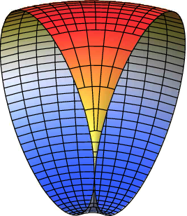
Since the shrinking area per plaquette on the inside of the torus necessitates a high density of dislocations we may approximate the dislocation cloud in this region by a continuous distribution of Burgers vector density $\bm{b}$. Minimizing the elastic energy with respect to $\bm{b}$ yields a variational equation from which the optimal dislocation density can be calculated as a function of the ratio $\epsilon_{d}/(YR^{2})$ between the dislocation core energy $\epsilon_{d}$ and elastic energy scale $YR^{2}$ with $R=R_{1}=R_{2}$.

As a starting point, we calculate the Green function $G_{L}(\bm{x},\bm{y})$ in the fat torus limit $r\rightarrow 1$ (i.e. $\kappa\rightarrow\infty$ and $\omega\rightarrow 0$, see Eq. (14)). The conformal angle $\xi$ in this limit is:

$$\lim_{r\rightarrow 1}\xi=\tan\frac{\psi}{2}\,,$$

and to leading order of $\kappa$ we have:

	$$\displaystyle\frac{\kappa}{16\pi^{2}}\left(\psi-\frac{2}{\kappa}\xi\right)^{2}\rightarrow\frac{\kappa}{16\pi^{2}}\,\psi^{2}-\frac{\psi}{4\pi}\tan\frac{\psi}{2}\,,$$
	$$\displaystyle\frac{\kappa}{4\pi^{2}}\Real\{\Li(\alpha e^{i\psi})\}\rightarrow\frac{\kappa}{16\pi^{2}}\,\psi^{2}+\frac{1}{2\pi^{2}}\log\left(\cos\frac{\psi}{2}\right)\,.$$

To handle the limit of the Jacobi theta function we can take $u=\Delta z/\kappa$, $q=e^{i\pi\tau}=e^{-\frac{2\pi}{\kappa}}$ and calculate the limit $q\rightarrow 1$. This can be done by using the modular transformation properties of Jacobi functions[30]:

$$\vartheta_{1}\left(\tfrac{u}{\tau}|-\tfrac{1}{\tau}\right)=-i(-i\tau)^{\frac{1}{2}}e^{\frac{iu^{2}}{\pi\tau}}\vartheta_{1}(u|\tau)\,.$$

(36)

Thus $\tau^{\prime}=-1/\tau=i\kappa/2$, $u^{\prime}=u/\tau=\Delta z/(2i)$ and $q^{\prime}=e^{i\tau^{\prime}}=e^{-\frac{\pi\kappa}{2}}$, where:

$$\lim_{q\rightarrow 1}\vartheta_{1}(u,q)=\lim_{q^{\prime}\rightarrow 0}i\left(\frac{i}{\tau^{\prime}}\right)^{-\frac{1}{2}}e^{\frac{iu^{\prime 2}}{\pi\tau^{\prime}}}\vartheta_{1}(u^{\prime},q^{\prime})\,.$$

This is easily evaluated by means of the expansion:

$$\vartheta_{1}(u,q)=2q^{\frac{1}{4}}\sin u+o\left(q^{\frac{9}{4}}\right)\,.$$

Taking the logarithm and neglecting irrelevant constant terms, we obtain:

$$\log\left|\vartheta_{1}\left(\frac{z-z^{\prime}}{\kappa}\Bigg|\frac{2i}{\kappa}\right)\right|\sim\log\left|\sinh\left(\frac{z-z^{\prime}}{2}\right)\right|\,,$$

which finally leads to:

$$G_{L}(\psi,\phi,\psi^{\prime},\phi^{\prime})\sim-\frac{\psi^{\prime}}{4\pi^{2}}\,\tan\frac{\psi^{\prime}}{2}\\ +\frac{1}{2\pi}\log\left|\sinh\left(\frac{z-z^{\prime}}{2}\right)\right|$$

(37)

with $z=\tan(\psi/2)+i\phi$. With the Green function in hand, we can calculate the effect of the curvature singularity at $\psi=\pi$ on the distribution of defects. Let $\bm{b}$ be the Burgers vector density of the dislocation cloud. Hereafter we work in a local frame, so that:

$$\bm{b}=b^{\psi}\bm{g}_{\psi}+b^{\phi}\bm{g}_{\phi}\,,$$

(38)

with $\bm{g}_{i}=\partial_{i}\bm{R}$ a basis vector in the tangent plane of the torus whose points are specified by the three-dimensional Euclidean vector $\bm{R}$. The quantity $\bm{b}$ has to be such that:

$$\int_{D}d^{2}x\,\bm{b}(x)=\bm{b}_{D}\,,$$

with $\bm{b}_{D}$ the total Burger’s vector in a generic domain $D$. Because on a closed manifold dislocation lines cannot terminate on the boundary, extending the integration to the whole torus we have:

$$\int d^{2}x\,\bm{b}(\bm{x})=0\,.$$

(39)

Since the basis vectors $\bm{g}_{i}$ in Eq. (38) have the dimension of length, contravariant coordinates $b^{i}$ have dimensions of an inverse area. Assuming all defects to be paired in the form of dislocations (i.e. $q_{i}=0$ everywhere), the total energy of the crystal reads:

$$F=\frac{1}{2Y}\int d^{2}x\,\Gamma^{2}(\bm{x})+\epsilon_{d}\int d^{2}x\,|\bm{b}(\bm{x})|^{2}\,,$$

(40)

where $\epsilon_{d}$ is the dislocation core energy and

$$|\bm{b}|^{2}=g_{ij}b^{i}b^{j}=g_{\psi\psi}(b^{\psi})^{2}+g_{\phi\phi}(b^{\phi})^{2}\,.$$

The function $\Gamma(\bm{x})$ encoding the elastic stress due to the curvature and the screening contribution of the dislocation cloud obeys

$$\frac{1}{Y}\Delta_{g}\Gamma(\bm{x})=\epsilon_{k}^{i}\nabla_{i}b^{k}(\bm{x})-K(\bm{x})\,,$$

(41)

where $\epsilon_{k}^{i}$ is the Levi-Civita antisymmetric tensor on the torus:

$$\epsilon_{\psi\phi}=-\epsilon_{\phi\psi}=\sqrt{g}\,,\qquad\qquad\epsilon_{i}^{j}=g_{ik}\epsilon^{jk}\,.$$

The stress function $\Gamma(\bm{x})$ can be expressed in the form $\Gamma(\bm{x})=\Gamma_{d}(\psi,\phi)-\Gamma_{s}(\psi)$ with

	$$\displaystyle\frac{\Gamma_{s}(\psi)}{Y}=\log\left[\frac{1}{2(1+\cos\psi)}\right]+1\,,$$		(42a)
	$$\displaystyle\frac{\Gamma_{s}(\psi,\phi)}{Y}=\int d^{2}y\,\epsilon_{k}^{i}\nabla_{i}b^{k}(\bm{y})\,G_{L}(\bm{x},\bm{y})\,.$$		(42b)

Taking advantage of the closeness of the torus we can integrate Eq. (42b) by parts so that:

$$\frac{\Gamma_{d}(\psi,\phi)}{Y}=-\int d^{2}y\,\epsilon_{k}^{i}b^{k}(\bm{y})\partial_{i}\,G_{L}(\bm{x},\bm{y})\,.$$

(43)

Now we want reduce the integral term in Eq. (43) to a more friendly functional of $\bm{b}$, suitable for a variational approach. Given the azimuthal symmetry we assume that all dislocations are aligned along $\bm{b}=b^{\phi}\bm{g}_{\phi}$. Even though not necessarily true, we argue this to be a reasonable work hypothesis as well as a solid starting point to capture the essential physics of the fat limit. In this case $\Gamma_{d}(\psi,\phi)=\Gamma_{d}(\psi)$ can be recast in the form

$$\frac{\Gamma_{d}(\psi)}{Y}=\frac{1}{2\pi}\int_{-\pi}^{\pi}d\psi^{\prime}\sqrt{g}\,b^{\phi}(\psi^{\prime})\\ \left[\psi^{\prime}+\sin\psi^{\prime}+\pi\sgn(\psi-\psi^{\prime})\right]\,.$$

(44)

Substituting Eq. (44) and (42a) in Eq. (40) and minimizing with respect to $b^{\phi}$ we can now write the variational equation:

	$$\displaystyle 4\epsilon_{d}R^{2}(1+\cos\psi)^{2}b^{\phi}(\psi)+\int_{-\pi}^{\pi}d\psi\,\sqrt{g}\,\Gamma_{d}(\psi^{\prime})\sgn(\psi-\psi^{\prime})$$
	$$\displaystyle=\int_{-\pi}^{\pi}d\psi\,\sqrt{g}\,\Gamma_{s}(\psi^{\prime})\sgn(\psi-\psi^{\prime})\,.$$		(45)

By inverting the order of integration in the integral on the right hand side, Eq (45) can be expressed in the form of a Fredholm equation of the second kind:

$$\lambda B(\psi)-\int_{-\pi}^{\pi}d\psi^{\prime}\,B(\psi^{\prime})\mathcal{K}(\psi,\psi^{\prime})=f(\psi)\,,$$

(46)

where $\lambda=\epsilon_{d}/(YR^{2})$, $B(\psi)=R^{2}(1+\cos\psi)^{2}b^{\phi}(\psi)$ and the kernel $\mathcal{K}(\psi,\psi^{\prime})$ is given by:

$$\mathcal{K}(\psi,\psi^{\prime})=\frac{1}{4(1+\cos\psi^{\prime})}\Bigg\{\pi^{-1}(\psi^{\prime}+\sin\psi^{\prime})(\psi+\sin\psi)\\ +|\psi-\psi^{\prime}|+2\cos\frac{\psi+\psi^{\prime}}{2}\sin\frac{|\psi-\psi^{\prime}|}{2}\Biggr\}\,.$$

(47)

The function $f(\psi)$ on the right hand side of Eq. (46) is given by:

	$$\displaystyle f(\psi)=-\frac{1}{4}\int_{-\psi}^{\psi}d\psi^{\prime}\,(1+\cos\psi^{\prime})\,\Gamma_{s}(\psi^{\prime})$$
	$$\displaystyle=\frac{1}{2}\bigl\{[\log 2(1+\cos\psi)-2]\sin\psi-2\Cl(\psi+\pi)\bigr\}$$		(48)

where $\Cl$ is the Clausen function (see Ref. 43, pp. 1005-1006) defined as:

$$\Cl(x)=-\int_{0}^{x}dx\,\log\left(2\sin\frac{t}{2}\right)=\sum_{k=1}^{\infty}\frac{\sin kx}{k^{2}}\,.$$

References

- [1] S.C. Glotzer, Some Assembly Required, Science 306, 419-420 (2004).
- [2] G.M. Whitesides and M. Boncheva, Beyond molecules: Self-assembly of mesoscopic and macroscopic components, Proc. Nat. Acad. Sci. USA 99, 4769-4774 (2002) [www.pnas.org/cgi/doi/10.1073/pnas.082065899].
- [3] J. K. Kim, E. Lee, Z. Huang and M. Lee, J. Am. Chem. Soc. 128, 14022 (2006).
- [4] E. J. Snijder and M. C. Horzinek, in The Coronaviridae, edited by S. G. Sidell, 219 (Plenum Press, New York, 1995)
- [5] J. Liu, H. Dai, J. H. Hafner, D. T. Colbert, R. E. Smalley, S. J. Tans and C. Dekker, Nature 385, 780 (1997).
- [6] V. Meunier, P. Lambin and A. A. Lucas, Phys. Rev. B 57, 14886 (1998).
- [7] C. P. Liu, H. B. Chen and J. W. Ding, J. Phys.: Condens. Matter 20, 015206 (2008).
- [8] M. Sano, A. Kamino, J. Okamura and S. Shinkai, Science 293, 1299 (2001).
- [9] A. Perez-Garrido, M. J. W. Dodgson, and M. A. Moore, Phys. Rev. B 56, 3640 (1997).
- [10] M. J. Bowick, D. R. Nelson and A. Travesset, Phys. Rev. B 62, 8738 (2000).
- [11] V. Vitelli, J. B. Lucks, and D. R. Nelson, Proc. Natl. Acad. Sci. USA 103, 12323 (2006).
- [12] L. Giomi and M. J. Bowick, Phys. Rev. B 76, 054106 (2007).
- [13] L. Giomi and M. J. Bowick, Phys. Rev. E 78, 010601(R) (2008).
- [14] D. R. Nelson and B. I. Halperin, Phys. Rev. B 19, 2457 (1979).
- [15] M. Do Carmo, Differential geometry of curves and surfaces, (Prenitce-Hall, Upper Saddle River, NJ, 1976).
- [16] S. A. Lavrenchenko, J. Math. Sci 51, 2537 (1990).
- [17] B. I. Dunlap, Phys. Rev. B 46, 1933 (1992); Phys. Rev. B 49, 5643 (1994); Phys. Rev. B 50, 8134 (1994).
- [18] S. Itoh, S. Ihara and J. Kitakami, Phys. Rev. B 47, 1703 (1993); Phys. Rev. B 47, 12908 (1993); S. Itoh and S. Ihara, Phys. Rev. B 48, 8323 (1993).
- [19] E. C. Kirby, Fullerene Sci. Tech. 2, 395 (1994).
- [20] I. László and A. Rassat, Int. J. Quantum Chem. 84, 136 (2001); J. Chem. Inf. Comput. Sci. 43, 519 (2003); I. László , A. Rassat, P. W. Fowler and A. Graovac, Chem. Phys. Lett. 342, 369 (2001).
- [21] M. V. Diudea, A. Graovac and A. Kerber, Commun. Math. Comput. Chem. 93, 102 (2001); M. V. Diudea, Phys. Chem. Chem. Phys. 4, 4740 (2002);
- [22] W. T Webber, Geometriae Dedicata 67, 31 (1997).
- [23] M. Goldberg, Tohoku Math. J. 43, 104 (1937).
- [24] D. L. D. Caspar and A. Klug, Cold Spring Harbor Symp. Quant. Bio. 27, 1 (1962).
- [25] H. S. M. Coxeter in A Spectrum of Mathematics (essay presented to H. G. Forder), edited by J. C. Butcher (Aukland University Press, Aukland, 1967), p. 98.
- [26] R. Saito, G. Dresselhaus and M. S. Dresselhaus, Physical Properties of Carbon Nanotubes (Imperial College Press, London, 1998).
- [27] P. Lambin, A. Fonseca, J. P. Vigneron, J. B. Nagy and A. A. Lucas, Chem. Phys. Lett. 245, 85 (1995); A. Fonseca, J. Hernadi, J. B. Nagy, P. Lambin and A. A. Lucas, Synth. Met. 77, 249 (1996).
- [28] Z. Yao, H. W. Ch. Postma, L. Balents and C. Dekker, Nature 402, 273 (1999).
- [29] J. Berger and J. E. Avron, Phys. Rev. A 51, 1146 (1995), J. Chem. Soc. Faraday. Trans. 91, 4037 (1995).
- [30] D. Mumford, Tata Lectures on Theta I (Birkhaüser, Boston, 1983); J. Polchinski, String Theory, Vol. I (Cambridge University Press, Cambridge, 1998).
- [31] M. Kleman and O. D. Lavrentovich, Soft Matter Physics, an Introduction (Springer, New York, 2003).
- [32] J. Han, Tech. Rep. NAS (1997); Chem. Phys. Lett. 282, 187 (1998).
- [33] M. J. Bowick, D. R. Nelson and A. Travesset, Phys. Rev. E 69, 041102 (2004).
- [34] A. R. Bausch, M. J. Bowick, A. Cacciuto, A. D. Dinsmore, M. F. Hsu, D. R. Nelson, M. G. Nikolaides, A. Travesset and D. A. Weitz, Science 299, 1716 (2003).
- [35] T. Einert, P. Lipowsky, J. Schilling, M. J. Bowick and A. Bausch, Langmuir 21, 12076 (2005).
- [36] D. R. Nelson, Nano Lett. 2, 1125 (2002).
- [37] F. C. Frank, Proc. R. Soc. London Ser. A 215, 43 (1952).
- [38] D. R. Nelson, Phys. Rev. Lett. 50, 982 (1983); M. Rubinstein and D. R. Nelson, Phys. Rev. B 28, 6377 (1983).
- [39] J. Kierfeld and V. Vinokur, Phys. Rev. B 61, R14928 (2000); Phys. Rev. B 69, 024501 (2004); J. Kierfeld, Physica C 300, 171 (1998).
- [40] D.P. Hardin and E.B. Saff, Adv. Math. 193, 174 (2005).
- [41] P. Pieranski, Phys. Rev. Lett. 45, 569 (1980).
- [42] L. Giomi and D. Giuliani, Toroidal Lattices Database, URL: http://physics.syr.edu/lgiomi/torus/database/.
- [43] M. Abramowitz and I. A. Stegun, Handbook of Mathematical Functions with Formulas, Graphs, and Mathematical Tables, (Dover, New York, 1964), URL http://www.math.sfu.ca/cbm/aands/.
- [44] L. Burakovsky, D. L. Preston and R. S. Silbar, Phys. Rev. B 61, 15011 (2000).
- [45] D. J. Wales and J. P. K. Doye, J. Phys. Chem. A 101, 5111 (1997).
- [46] S. Goedecker, J. Chem. Phys. 120, 9911 (2004).
- [47] W. H. Press, S. A. Teukolsky, W. T. Vetterling and B. P. Flannery Numerical Recipes in C, (Cambridge University Press, Cambridge, 1992), 2nd Edition.
- [48] R. A. Dwyer, Algorithmica 2, 137 (1987).